
Nonuniformity of Isometric Properties of Automotive Driveshafts


1
Department of Mechanics, University POLITEHNICA of Bucharest, 060042 Bucharest, Romania
2
New Technology Network-Société Nouveau des Roulements (NTN-SNR), 002400 Sibiu, Romania
*
Author to whom correspondence should be addressed.
Computation 2021, 9(12), 145; https://0-doi-org.brum.beds.ac.uk/10.3390/computation9120145
Submission received: 15 November 2021
/
Revised: 10 December 2021
/
Accepted: 15 December 2021
/
Published: 20 December 2021
(This article belongs to the Special Issue Experiments/Process/System Modeling/Simulation/Optimization (IC-EPSMSO 2021))
Abstract
:This paper presents an analysis of the CVJ (constant velocity joint) of automotive driveshafts from a point of view concerning the nonuniformity of isometric properties. In the automotive industry, driveshafts are considered to have constant velocity through its joints: free tripode joints and fixed ball joints, which has been proved by Mtzner’s indirect method and Orain’s direct method for tripod joint. Based on vectorial mechanics, the paper proved the quasi-isometry of velocity for polypod joints such as fixed ball joints. In the meantime, it was computed that the global nonuniformity of constant velocity joints for modern driveshafts based on the Dudita-Diaconescu homokinetic approach for the driveshafts. The nonuniformity of the velocity isometry of driveshafts was computed as a function of the input angular velocity of the driveshaft, angular inclination between the tripod–tulip axis and the midshaft axis and the angular inclination between the bowl axis and midshaft axis. The main aim of this article is how to improve the geometric and kinematic approach to add an important correction when designing the driveshaft dynamics prediction such as: forced torsional vibrations, forced bending–shearing vibrations, and coupled torsional–bending vibrations for the automotive driveshaft in the regions of specific resonances such as principal parametric resonance, internal resonance, combined resonance, and simultaneous resonances. By the way it is added, there are important corrections for the design of driveshafts, for the torsional dynamic behavior prediction, and for bending–shearing dynamic behavior of the driveshafts in the early stages of design. The results presented in the article represent a starting point for future research on dynamic phenomena in the area mentioned previously.
1. Introduction
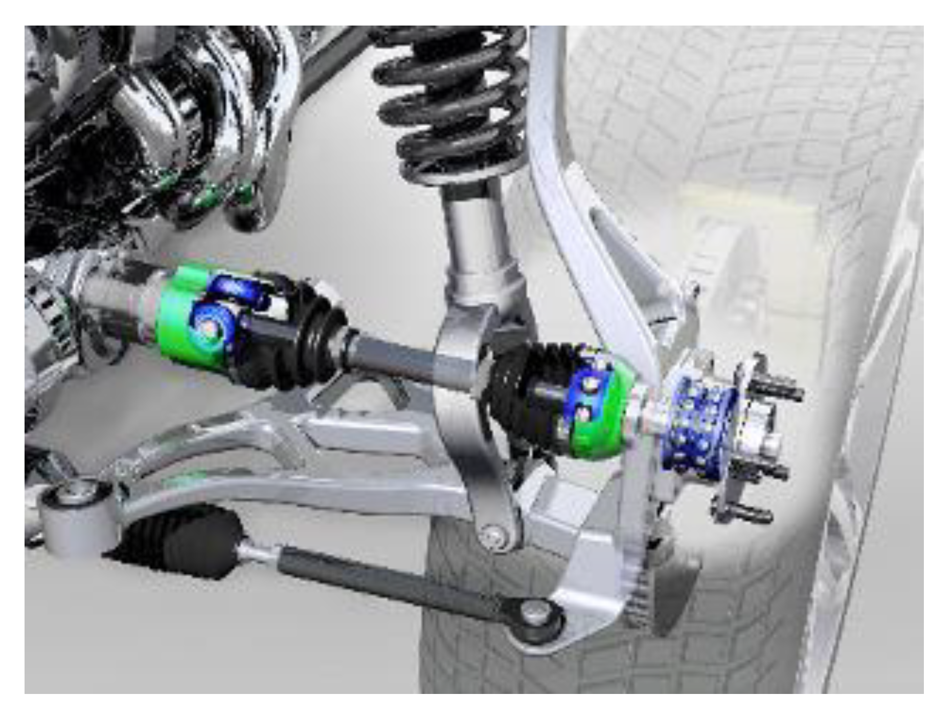
The constant velocity joints (CVJs) for automotive driveshafts are special mechanisms that transmit the load torque by angular rotation from the gear box to the wheels of a car as can be seen in Figure 1. In the development of the car industry, the concerns are the capability of this kind of transmission to have isometric properties from a geometric versus kinematic point of view and from a dynamic torque transmission point of view as mentioned in literature [1].
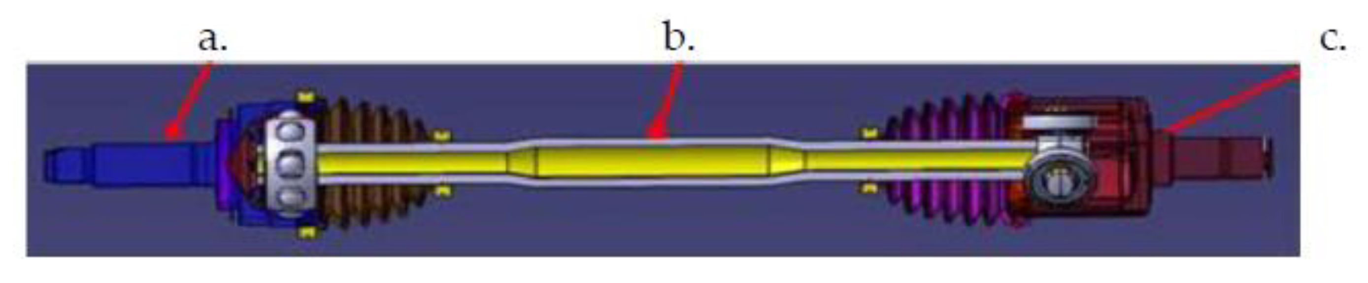
For a better understanding, let us look inside the components of such a mechanism by looking at the Figure 2, which consists of (a) the bowl-balls joint fixed assembled by the car wheel; (b) the midshaft axis; (c) the tulip–tripode joint that allows for axial plunging of the tripod in the tulip and the plunging assembled in the gear box.
Over the last four decades, the kinematics and the torque loads of this transmission system was considered isometric due to the introduction of the Rzeppa joint, in the 1970 by Glenzer, and by using tripod plunging joints in the tulip and fixed ball joints in the bowl in the 19890s [2,3,4]. This way, starting with the last decade of the last century, it was considered that bowl–balls joints and the tulip–tripod joints were CVJs (constant velocity joints), it means isometric with respect to kinematics and isometric with respect to the torque loads. While the last aspect is true (and the practice demonstrates it), the isometry from a kinematics point of view is not true, this aspect being known as quasi-isometry kinematics for automotive driveshafts [1] (p. 78) and [5]. The literature, especially in Journals published by MDPI, is very poor on presenting such subjects, not because it is less important for the design area and for the automotive industry, but because it involves a huge investment in experimental research and most of research is linked to intellectual property through the patents held by the biggest corporations in the car industry such as Renault, Daimler–Benz, BMW, GMC, Chrysler, and Audi–VW Group. In the literature, an active steering control strategy to prevent rollover of a vehicle [6] or a hierarchical synchronization control strategy for the ARIS system to overcome the synchronization errors induced by the wheels have been highlighted [7]. As can be seen, none of this research has involved the nonuniformity of the geometric and kinematic isometry of automotive driveshafts. Tiberiu-Petrescu mentioned in [8] the variation in angular velocity of a double-cardan transmission, while in [9], it dealt with the use of a six-sigma methodology for the optimization of cardan shaft transmission for light truck driveshafts, because it’s exploitation was necessary for improving the vibration’s noise harshness. One paper [9] mentioned the presence of vibration noise harshness due to the driveshaft, but the authors did not research why this phenomenon was present. In one researcher’s master’s thesis [10], the author developed a software based on MATLAB’s Simulink to realize the modeling and simulation of vehicle kinematics and dynamics, but the models of vehicle transmission are very simple without touching the special phenomena of vehicle transmission. The paper [11] present a design and a stress analysis for an automobile driveshafts made of composites material for scientists trying to avoid special phenomena that is not well explained by the transmission’s designers. The first researchers who considered special phenomena for driveshafts were Mazzei and Scott, who enhanced the nonlinear parametric dynamic behavior of a universal joints in [12]. What is very strange for this research paper is that it contains only two references: of which one is a self-citation in the same field of dynamic stability of shafts driven through a universal cardan joint. The experimental evidence on the nonuniformity of CVJ driveshaft transmissions is presented and high-lighted by Browne and Palazzolo in the paper [13]. But the most important experimental research on the nonuniformity of geometric and kinematic isometry of CVJ driveshafts was carried out by Steinwede during his PhD thesis [14] (pp. 68–97); thus, after 45 years, it was finally proven through experimental data that Dudita and Diaconescu were right, that CVJ driveshafts are quasi-homokinetic, and all the designed patents and design flow charts used in the automotive industry concerning CVJ driveshafts must be modified and corrected as already was mentioned in [1] (p. 78). In addition, Feng, Rakheja, and Shangguan in [15] treated the optimization of the generated axial force (GAF) of a driveshaft system with an interval of uncertainty without considering the CVJ’s isometry for the driveshaft, which is no longer isometric, as this aspect was certified by experiments using the vertex method for the analysis of the upper and lower bonds (ULBs) variation of parameters. It is clear now that the nonuniformity of geometric and kinematic isometry of driveshafts represents the starting point of all the research concerning design, analysis, and dynamic investigation of the behavior of automotive driveshafts. This paper highlights this nonuniformity from isometry of geometry and kinematics for CVJ automotive driveshafts.
2. State of the Art
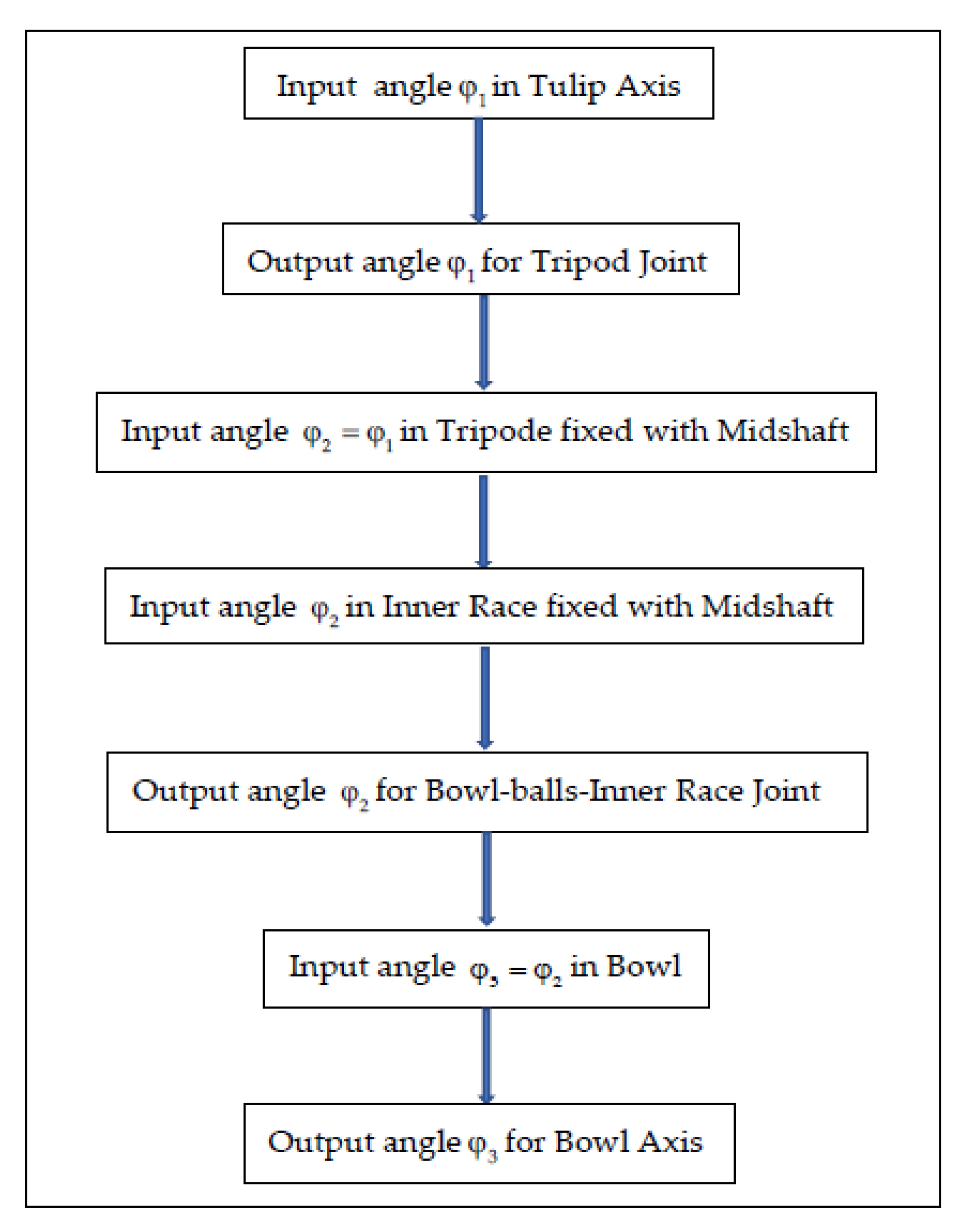
The first to introduce the concept of a CVJ was Metzner, in 1967, who is mentioned in the literature [4] as the creator of the first indirect method (FIM) for proving constant velocity for special Hooke joints [1], based on the idea that “the generators of a constant velocity joint must be mirror images in space” [1] (p. 61). Figure 3 highlight the functioning through a flow chart of a CVJ automotive driveshaft.
Presented in detail in Figure 4 is a tripod that consists of three pods equally fixed inclined, with respect to the midshaft of the automotive driveshaft with the fixed angles, .
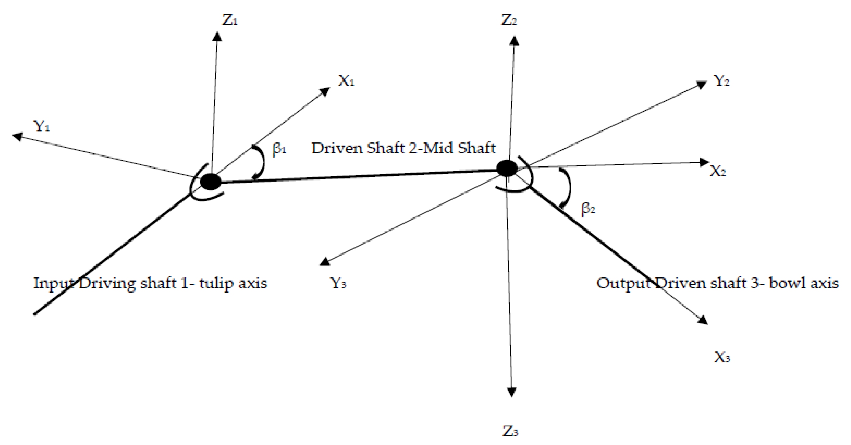
In Figure 5, presented is a schematic representation of an automotive drive shaft in three Cartesians systems with the coordinates X1,Y1,Z1 attached to the tulip, X2,Y2,Z2 attached to the midshaft, and X3,Y3,Z3 attached to the bowl, having the next rigid movements:
- -
- Rotation with the angle φ1 of the tulip with respect to the X1, φ1 = 0 … n1π;
- -
- Rotation with the angle φ2 of the midshaft with respect to the X2, φ2 = 0 … n1π;
- -
- Rotation with the angle φ3 of the bowl with respect to the X3, φ3 = 0 … n1π;
- -
- Relative rotation of the longitudinal axe of the midshaft (given by the direction of the axis X2) with respect to the longitudinal direction of the tulip (given by the direction of the axis X1), with β1 (spatial angle between axis X1 and X2) with respect to the axis Z1, β1 being the angle between longitudinal direction of the tulip and the longitudinal direction of the midshaft, β1 = 0° … 15°;
- -
- Relative rotation of the longitudinal axis of the bowl (given by the direction of the axis X3) with respect to the longitudinal direction of the midshaft (given by the direction of the axis X2), with β2 (spatial angle between axis X2 and X3) with respect to the axis Y2, β2 being the angle between the longitudinal direction of the midshaft and the longitudinal direction of the bowl, β1 = 0° … 47°.
Using all these notations, Orain proved, in 1976, using the second direct method [16] that the polypod joints, the tripod joints, are isometric joints from the kinematic and dynamic points of view, the kinematic point of view being expressed by the Relations:
It means the tripode joint that is a tulip–tripod joint is a CVJ, but, in 1975, Dudita and Diaconescu [5] proved that the tripode joint is quasi-isometric, a fact that was only recognized by researchers in the field [1] (p. 78) until 2006. At that time, in the nineteen-seventies, it was considered that a nonuniformity from a kinematic isometry of the tripode joints of 5–7% was acceptable; now, when an improvement of 1% is a huge gain in the automotive industry, and is it is no longer acceptable. Thus, the homokinetic transmission of the driveshafts, it is in fact quasi-homokinetic; therefore, for the early stages of design in the automotive industry, it is necessary to express and evaluate the kinematic and geometric isometric nonuniformities of the driveshafts as well as their implications in the dynamic behavior of the transmission. In addition, the bowl-balls joint has not proven to be a CVJ.
3. Proving the Constant Velocity of the Bowl-Balls Joint
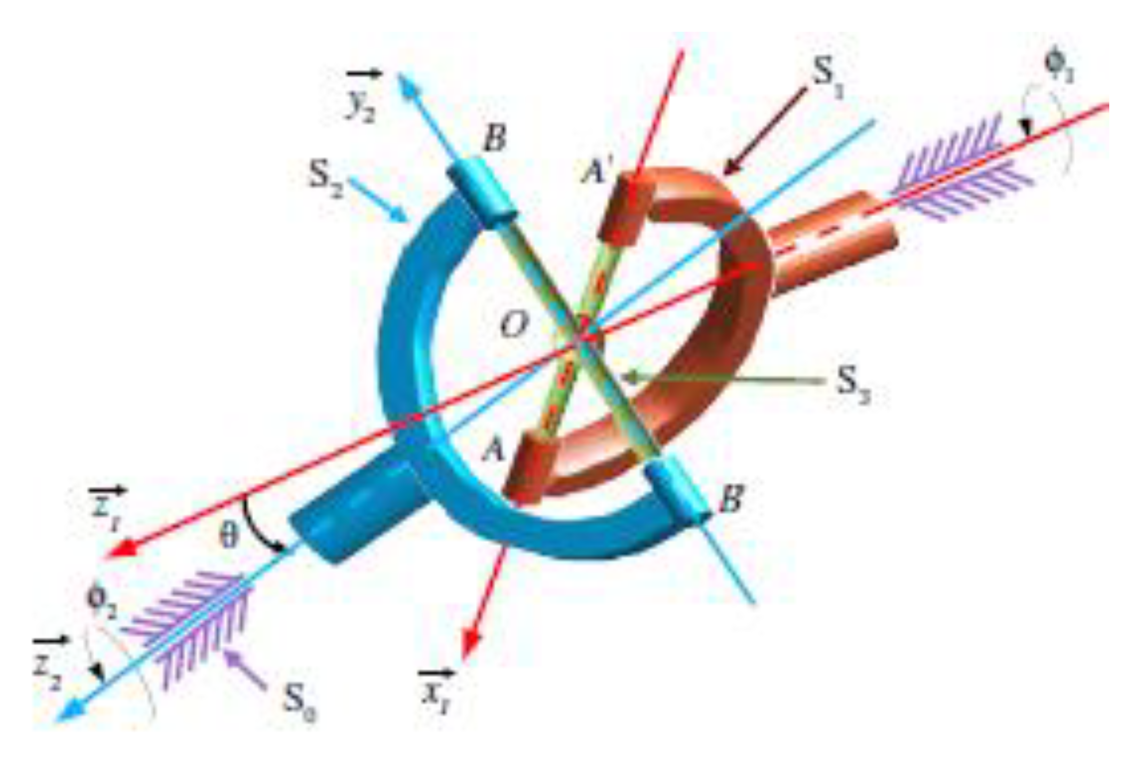
Let us consider a general cross Hooke joint as presented in Figure 6, where the driving element is S1, having attached to the cartesian system R1(OX1,Y1,Z1), the driven element is S2, having attach the cartesian system R2(OX2,Y2,Z2); the cross joint is A’OA-B’OB, having the angle , the driving input angle is , the driven output angle is , and the angle between the longitudinal direction of the input element S1 and the longitudinal direction of output element S2 is θ.
We can consider three-unit vectors , , so that we have the Relations:
that yield to express the unit vectors of and as:
Based on Equations (7) and (8) yields:
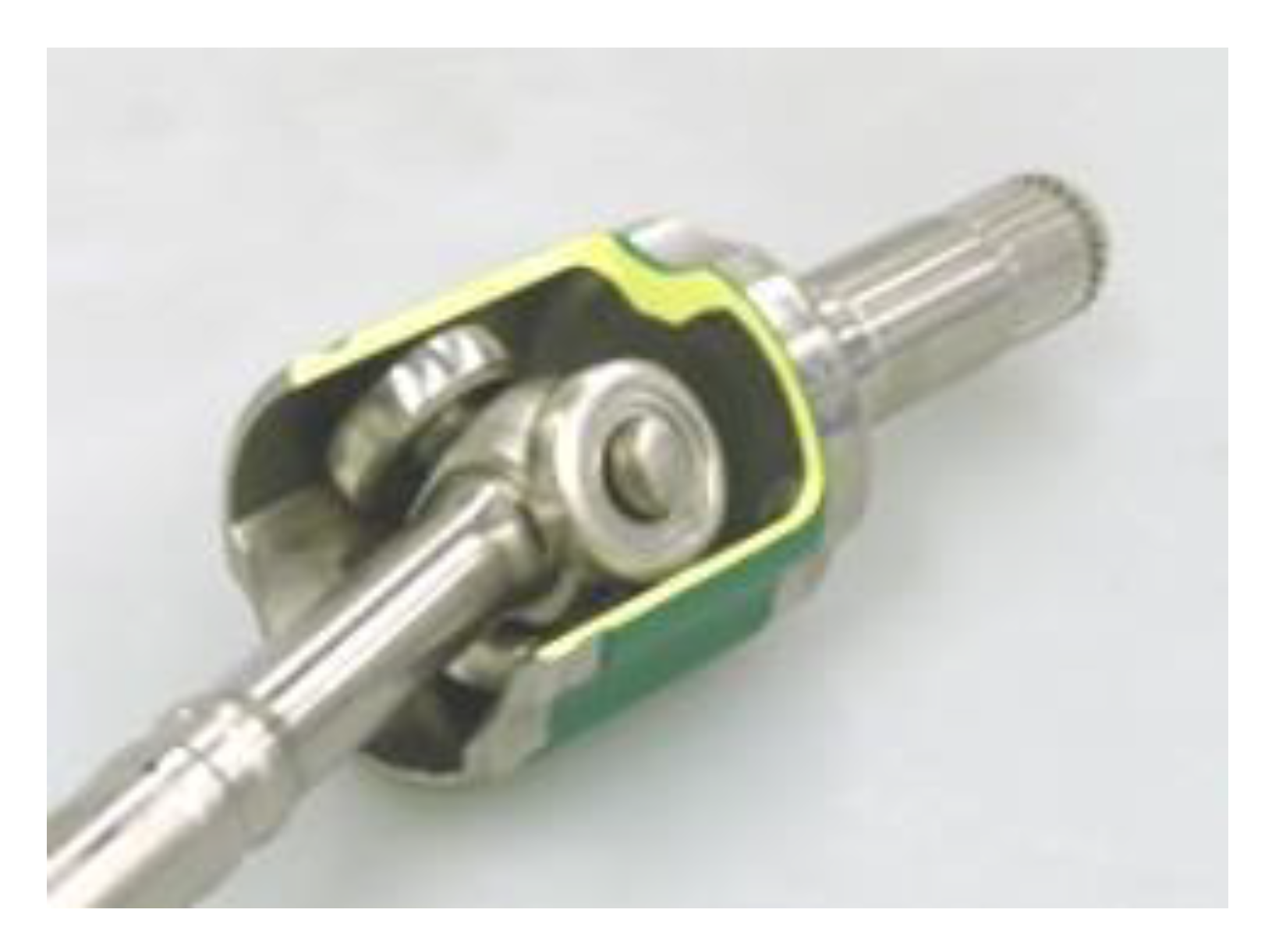
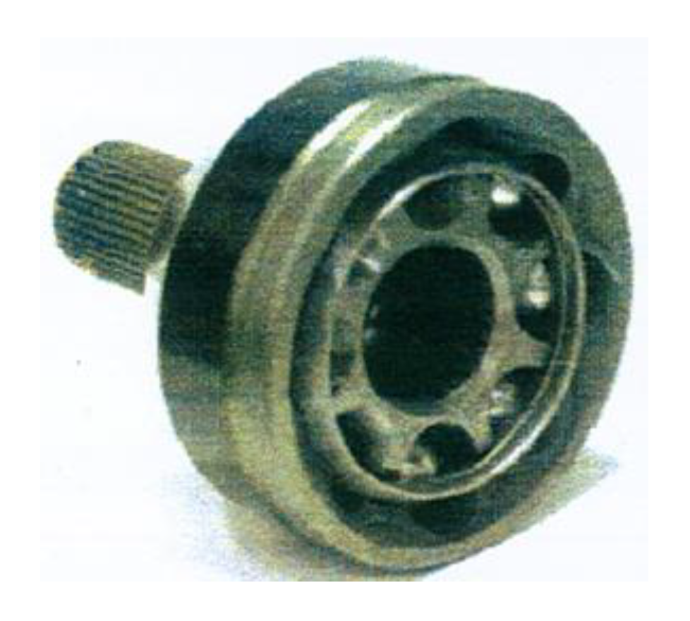
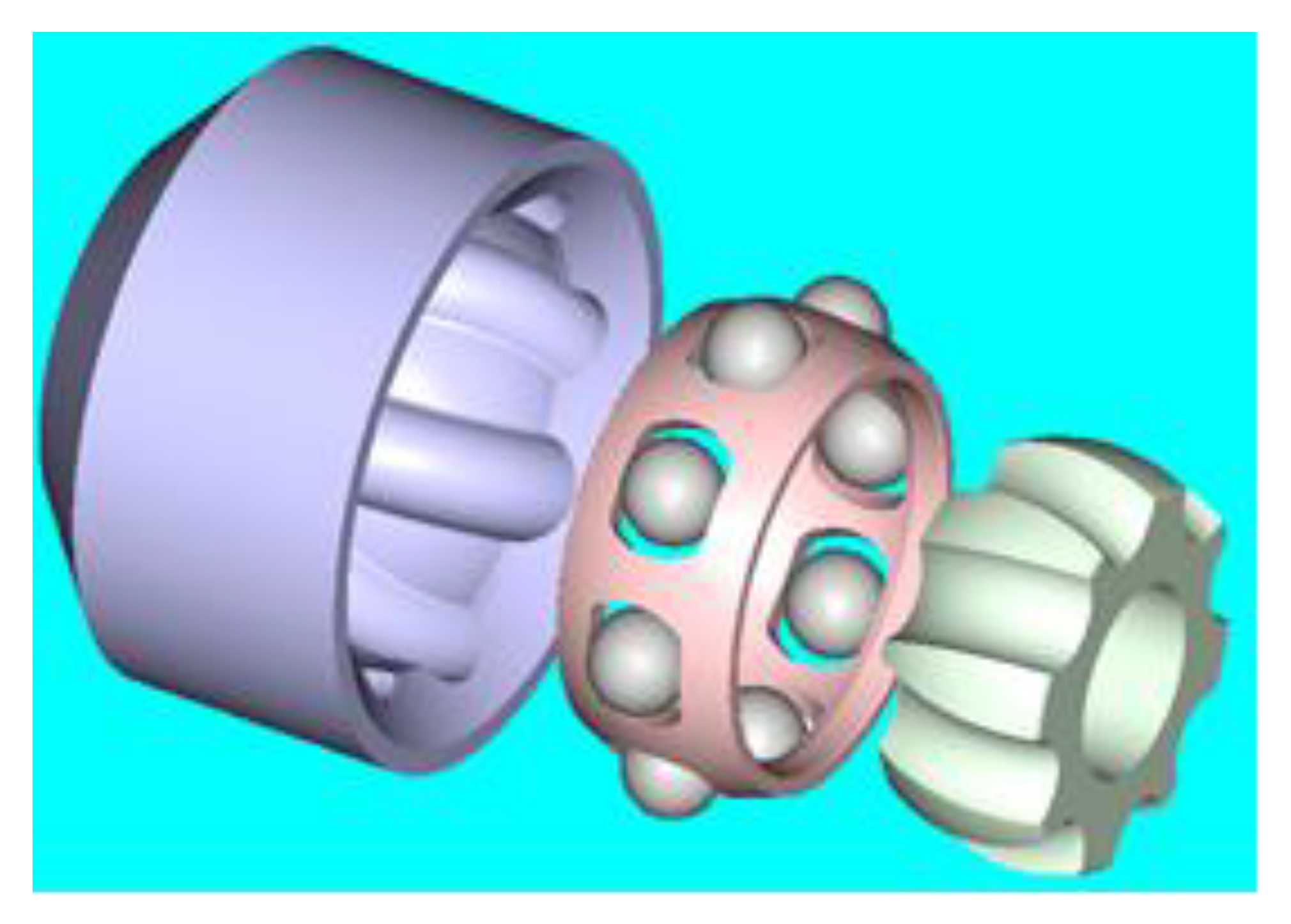
The most common number of balls for a bowl-balls joint is six, so using Equation (10) for the bowl-balls joint (see Figure 7 and Figure 8), putting and for given by Relation:
where is the numbers of balls of the bowl-balls joint that must be multiples of 3 (condition of homokinetic driveshaft joint), yields the relations:
- for the bowl-balls joint considering all the balls 1–3–5 like a tripode joint:
- -
- for the first transmitting ball element: Ψ1 = 0°:
- -
- for the third transmitting ball element: Ψ3 = 120°:
- -
- for the fifth transmitting ball element Ψ5 = 240°:Equations (12)–(14) are identical to those of the tripode joint therefore it is obtained
- for the bowl-balls joint considering all the balls 2-4-6 like a tripode joint:
- -
- for the second transmitting ball element Ψ2 = 60°:
- -
- for the fourth transmitting ball element Ψ4 = 180°:
- -
- for the sixth transmitting ball element Ψ6 = 300°:
Equations (16)–(18) lead to the same solution (15); therefore, considering Equation (4) yields the geometric isometry meaning that both joints of the automotive driveshaft have kinematic isometry. In fact, considering the aspects found by Dudita and Diaconescu [5], we can consider that from a kinematic point of view, we have a quasi-isometry of the geometric and kinematic of the automotive driveshafts.
4. Nonuniformity of Geometric vs. Kinematic Isometry of Driveshafts and Discussions
The relations that express the nonuniformity of the kinematic isometry of driveshafts can be obtained from the general formulation found by Dudita and Diaconescu [5] for an input driving shaft with rigid rotation angle and an output driven shaft with rigid rotation angle are:
where r is the radius of the joint, l is the length of the driven shaft, and β is the angle between the longitudinal directions of the two shafts. With the signification of the terms mentioned before yields:
- -
- for the tulip–tripode joint:
- -
- for the bowl-balls joint:where r1 is the tulip radius, r2 is the bowl radius, and l is the length of the midshaft. After injecting the Relation (20) in (21) yields:And the dependance of the angular speed of the bowl with respect to the angular speed of the tulip is:
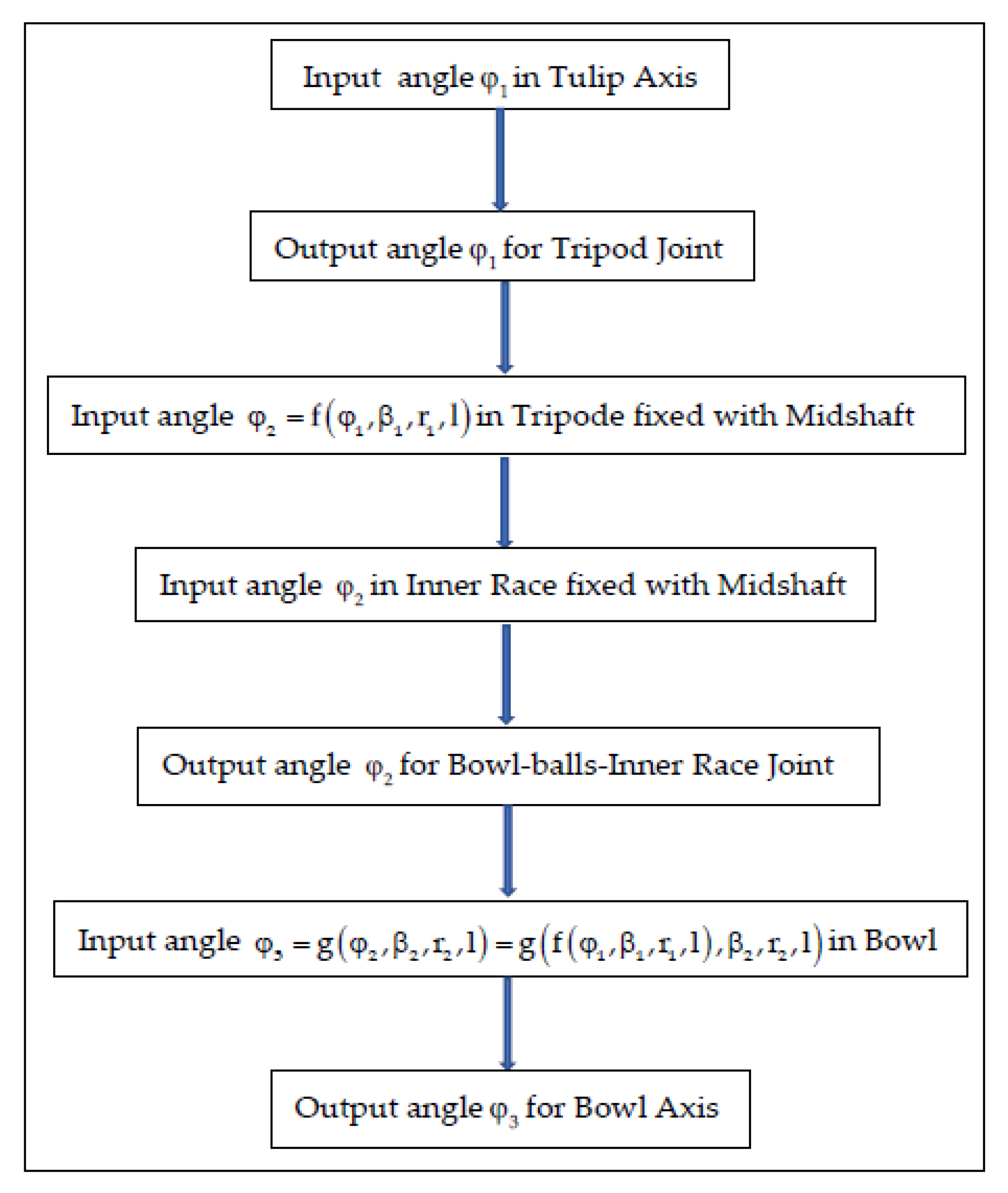
In Figure 9 presents a flow chart of a quasi-isometric CVJ automotive driveshaft.
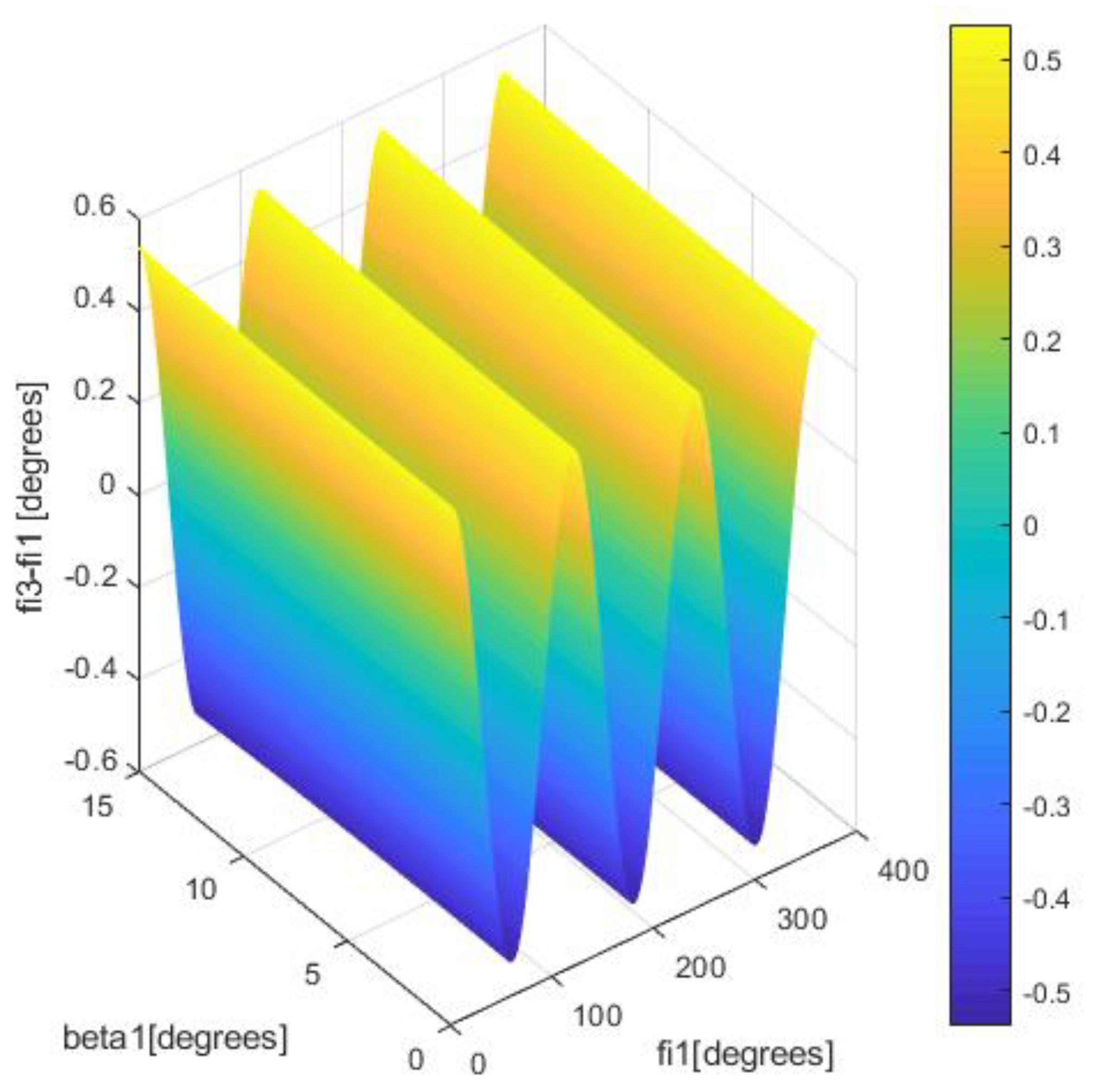
Based on Relation (22), the software in MATLAB was used to compute the geometric nonuniformity of the geometric isometry for the driveshaft as a function of β1, β2 and φ1 as can be seen in Figure 10 and Figure 11.
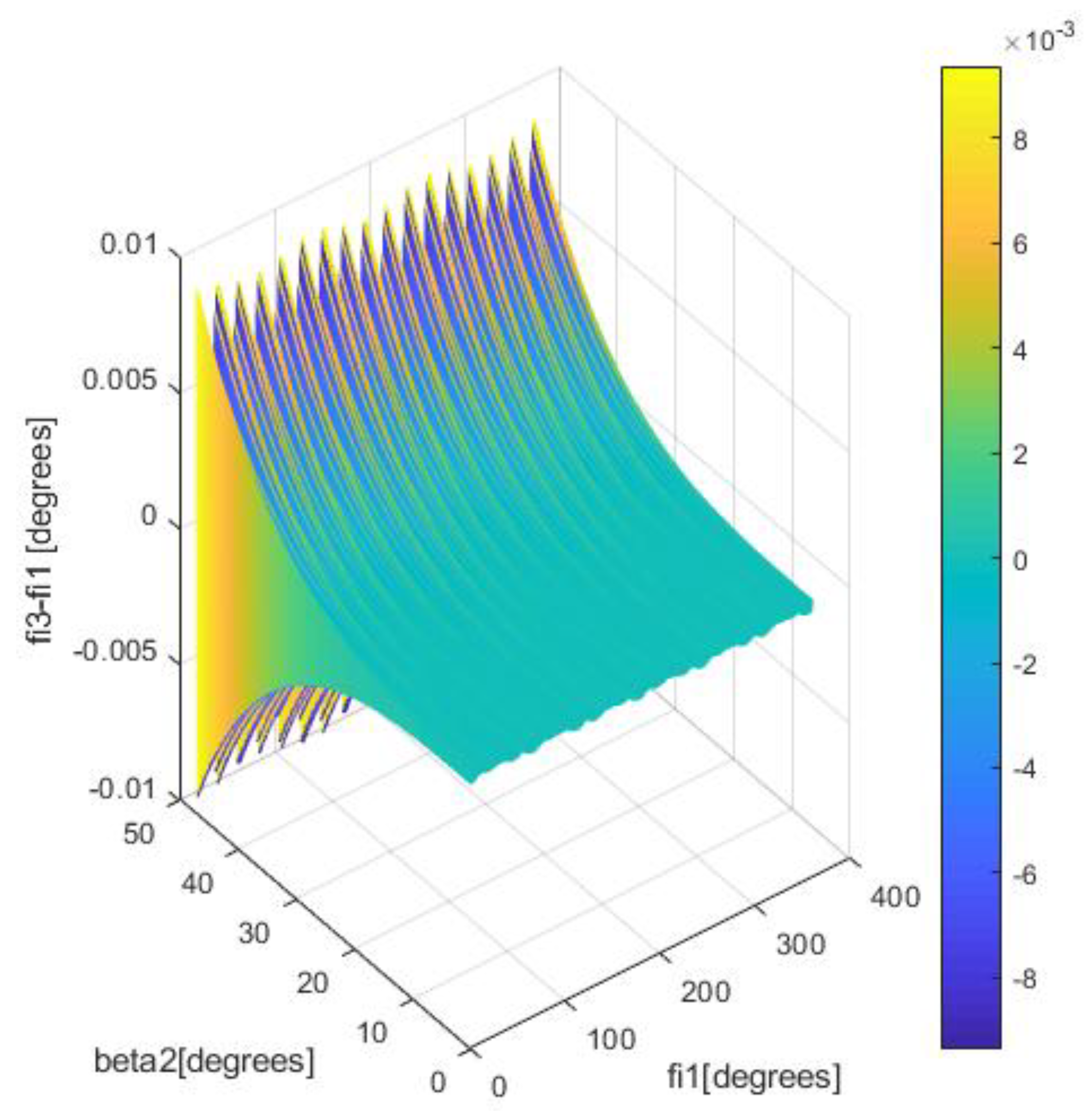
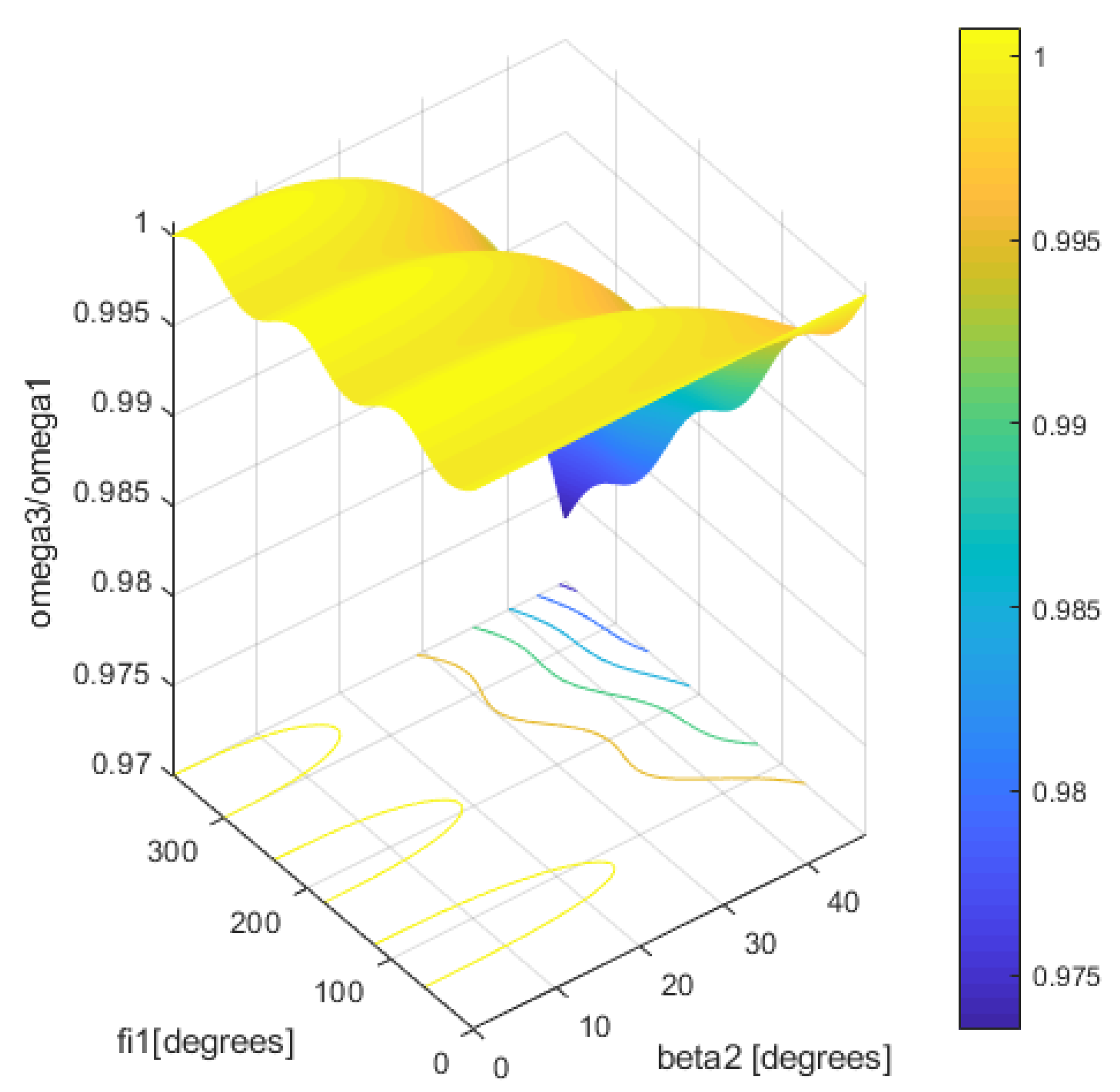
Analyzing these figures, it can be concluded that the geometric nonuniformity of isometry was in the range ±0.009° being maximum when β2 has the maximum value of 47°. Comparing these results with the experimental data in the literature [14] (pp. 70–71), it can be remarked that it had close agreement. In addition, Steinwede in [14] (pp. 88–94) experimentally demonstrated that this geometric nonuniformity of isometry for a driveshaft is the principal cause of premature pitting on the flanks of the tripod, on the internal flanks of the tulip, on the balls of the bowl-inner race joint, and on the internal flanks of the bowl due to the insufficient design for controlling Hertzian contact with respect to phenomena that involves geometric nonuniformity of isometry involving the driveshaft. Using Relation (23), a software in MATLAB was developed to compute the kinematic nonuniformity of isometry for the driveshaft as a function of β1, β2, and φ1 as can be seen in Figure 12 and Figure 13.
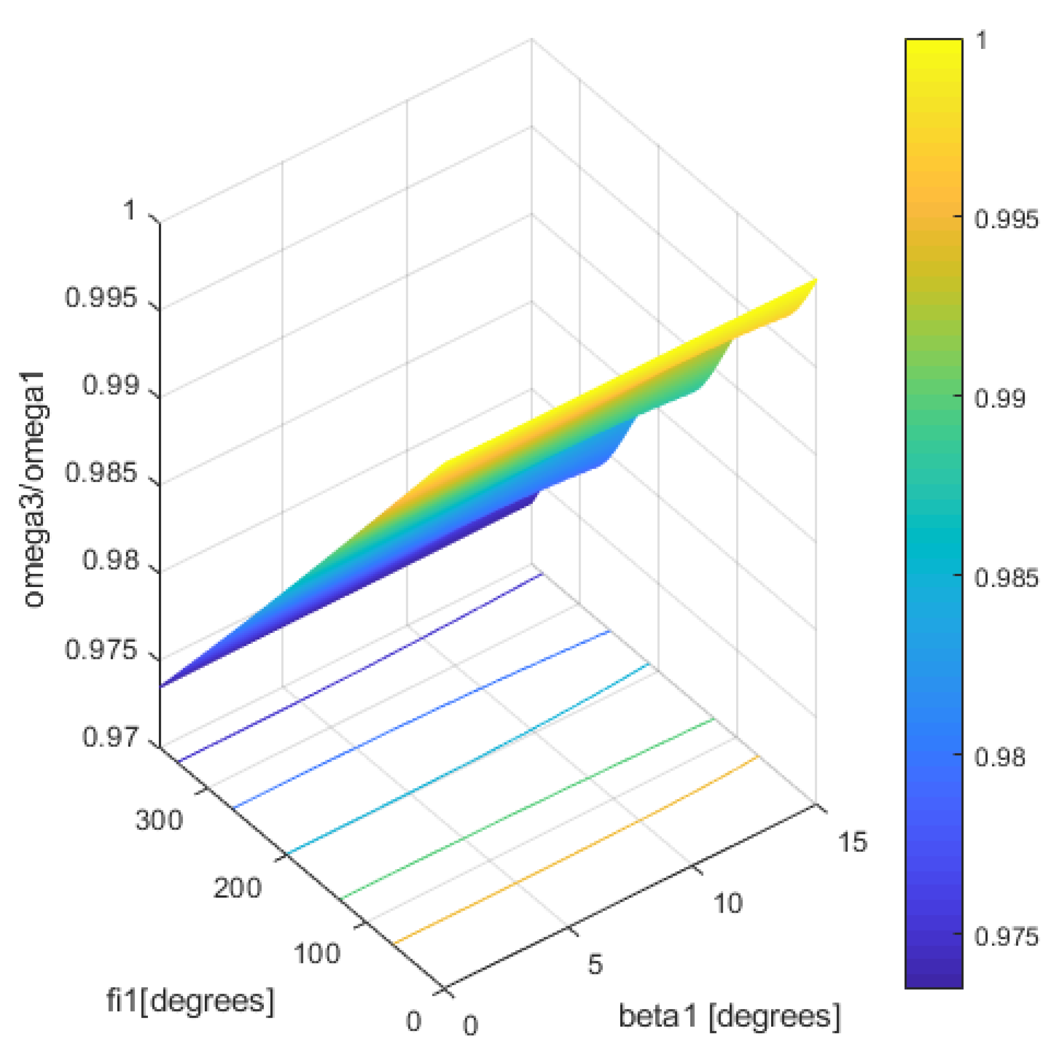
Analyzing Figure 12, it can be remarked that the kinematic nonuniformity of the isometry for the driveshaft, when β2 = 47° and β1 is in the range 0–15°, is in the range (−0.027, 0), having maximum absolute values for = 93°, 213°, and 325°, while the minimum absolute values were obtained for = 33°, 151°, and 271°. Regarding Figure 13 it can be concluded that that the kinematic nonuniformity of the isometry for the driveshaft, when β1 = 15° and β2 is in the range 0–47°, was in the field (−0.024, 0.001) having maximum value for φ1 = 76°, 190°, and 316° while the minimum values were obtained for φ1 = 31°, 169°, and 258°.
In Figure 14, the geometric nonuniformity isometry for the driveshaft as a function of β1 and β2, being variables, and . As can be remarked from Figure 14, the geometric nonuniformity isometry for the driveshaft was maximum for β2 = 47° regardless of the variation in β1 in the range 0–15°. From the perspective of the last simulation concerning the geometric nonuniformity isometry for the driveshaft, it can be concluded a great sensitivity for the maximum angle β2 of the longitudinal direction of the bowl with respect to the midshaft longitudinal direction. From the design point of view, this aspect involved a sensitivity to shocks received from the wheel of the driveshafts even if the value of nonuniformity was very small.
In addition, analyzing Figure 10, Figure 11, Figure 12 and Figure 13, the harmonic fluctuation of the nonuniformity from the geometric and kinematic isometry of the automotive driveshaft can be highlighted. This is a challenge for the driveshaft’s designers because of the difficulty of predicting the supplementary quantities for the fatigue solicitations. Moreover, the harmonic fluctuation of the nonuniformity from geometric and kinematic isometry of the automotive driveshaft induces the nonlinear parametric dynamic behavior of a CVJ as mentioned in [12]. All this geometric and kinematic nonuniformities from the isometry of automotive driveshafts must be considered in the design patents for automotive driveshafts such as in [17,18,19,20]. These aspects of considering the automotive driveshafts as quasi-isometric (isometry with nonuniformity) CVJ (homokinetic) transmissions allows for the development of future research in torsional forced vibrations and the bending–shearing vibrations of automotive driveshafts. This starting point in the investigation of the geometric and kinematic isometric nonuniformities of driveshafts opens the door to modeling of the forced torsional dynamic behavior of the driveshafts in the region of nonlinear parametric vibrations as already mentioned in literature [9,12,13,14] as future research, especially in the regions of:
- -
- primary resonance for excitation frequency, [21] (p. 196);
- -
- super harmonic resonance for excitation frequency, , k1 positive integer [21] (p. 211);
- -
- subharmonic resonance for excitation frequency, k1 positive integer [21] (p. 214);
- -
- principal parametric resonance for excitation frequency, [21] (p. 425);
- -
- combination resonances for excitation frequencies, [21] (pp. 202, 430);
- -
- simultaneous resonances for excitation frequencies, , with k positive integer [21] (p. 188);
- -
- internal resonances for with k1 and k2, positive integers [21] (p. 381).
5. Conclusions
The paper highlights the geometrical and the kinematic nonuniformities of the isometry for the automotive driveshaft. The geometrical nonuniformities of the isometry for the automotive driveshaft was in the range ±0.009°, while the kinematic nonuniformities of the isometry for the automotive driveshaft was in the range (−0.027, 0.001). This was not in accordance with the classic design published in literature [1] (p. 78), because the maximum angles between the tulip axis and the midshaft axis is now in the current car industry β1 = 15°, and the maximum angle between the midshaft axis and bowl axis is β2 = 47°, while in design literature [1] (p. 78), these angles are considered less than 10°, so it is mentioned, by Seherr-Thoss [1], that the geometrical nonuniformity for the isometry of driveshaft is maximum 0.0000675°, that is, “within the manufacturing tolerances of CVJ”. This last conclusion is no longer valid, as Steinwede experimentally demonstrated in his PhD Thesis [14] (pp. 70–71), and, therefore, the Relation (20), mathematical demonstrated by Dudita and Florescu in [5], is more than ever necessary in the design for automotive driveshafts and represents a correction needed to be applied to most of the patent’s design such as in [17,18,19,20]. The maximum values of the isometric nonuniformity are obtained when β2 has a maximum value of 47°; therefore, this paper highlights the sensitivity of the driveshaft to the excitations received from the wheel. As can be seen from all the aspects of this paper, automotive driveshafts do not have perfect geometric and kinematic isometry, even if the tulip–tripode joint and bowl-balls joint represent, in view of technological developments over the last four decades, the most advanced homokinetic transmissions. The prediction of geometric and kinematic isometry nonuniformity of the driveshaft represent a powerful tool for designers because it allows for prediction in the early design stages of the automotive driveshaft, the prediction of resonances such as super harmonic resonance, subharmonic resonance, principal parametric resonance, combination resonances, simultaneous resonances and internal resonances. Also, this aspect allows the investigation of stability in these specific resonances ranges for the nonlinear parametric dynamic behavior of the automotive driveshaft. These phenomena have of a huge importance when establishing the dynamic behavior of the automotive transmission from the gearbox to the wheel. Finally, it can be concluded that this paper introduces an important correction for the design of automotive driveshafts, for the torsional dynamic behavior prediction, and for bending–shearing dynamic behavior prediction of the driveshafts in the early stages of design. The results presented in the article is a starting point for the future research of dynamic phenomena in the area mentioned previously.
Author Contributions
Conceptualization, M.B. and A.V.; methodology, M.B. and A.V.; software, M.B.; validation, M.B.; formal analysis, M.B.; investigation, M.B.; resources, M.B. and A.V.; data curation, M.B.; writing—original draft preparation, M.B.; writing—review and editing, M.B.; visualization, M.B.; supervision, M.B.; project administration, M.B. All authors have read and agreed to the published version of the manuscript.
Funding
This research received no external funding.
Institutional Review Board Statement
Not applicable.
Informed Consent Statement
Not applicable.
Data Availability Statement
Not applicable.
Acknowledgments
The authors of this article are thankful to the University POLITEHNICA of Bucharest for provide a serene environment and facilities to carry out this research work.
Conflicts of Interest
The authors declared no potential conflict of interest with respect to the research, authorship, and/or publication of this article.
References
- Seherr-Thoss, H.C.; Schmelz, F.; Aucktor, E. Theory of Constant Velocity Joints (CVJ). In Universal Joints and Driveshafts, 2nd ed.; Springer: Berlin, Germany, 2006; pp. 53–80. [Google Scholar]
- Patent Rzeppa. Available online: https://worldwide.espacenet.com/patent/search/family/008989560/publication/FR628309A?q=pn%3DFR628309A (accessed on 3 March 2020).
- Glaenzer-Spicer. Tripod Joint GI. European Patent No. 1.272.530, 4 July 1960. [Google Scholar]
- Schmelz, F.; Seherr-Thoss, H.C. Die Entwicklung der Gleichlaufgelenke fur den Frontantrieb; VDI-Report No. 418; VDI: Ingolstadt, Germany, 1981. [Google Scholar]
- Duditza, F.; Diaconescu, D. Zur Kinematik und Dynamik von Tripode-Gelenkgetrieben. Konstruction 1975, 27, 335–341. [Google Scholar]
- Shao, K.; Zheng, J.; Huang, K.; Qiu, M.; Sun, Z. Robust model referenced control for vehicle rollover prevention with time-varying speed. Int. J. Veh. Des. 2021, 85, 48–68. Available online: https://www.inderscienceonline.com/doi/abs/10.1504/IJVD.2021.117154 (accessed on 7 December 2021). [CrossRef]
- Deng, B.; Zhao, H.; Shao, K.; Li, W.; Yin, A. Hierarchical Synchronization Control Strategy of Active Rear Axle Independent Steering System. Appl. Sci. 2020, 10, 3537. [Google Scholar] [CrossRef]
- Tiberiu-Petrescu, F.I.T.; Petrescu, R.V.V. The structure, geometry, and kinematics of a universal joint. Indep. J. Man ana Prod. 2019, 10, 1713–1724. [Google Scholar] [CrossRef]
- Ertürka, A.T.; Karabayb, S.; Baynalc, K.; Korkutd, T. Vibration Noise Harshness of a Light Truck Driveshaft, Analysis and Improvement with Six Sigma Approach. ACTA Phys. Pol. A 2017, 131, 477–480. [Google Scholar] [CrossRef]
- Kamalakkannan, B. Modelling and Simulation of Vehicle Kinematics and Dynamics. Master’s Thesis, Halmstad University, Halmstad, Sweden, 13 January 2017. [Google Scholar]
- Kishore, M.; Keerthi, J.; Kumar, V. Design and Analysis of Drive Shaft of an Automobile. Int. J. Eng. Trends Technol. 2016, 38, 291–296. [Google Scholar] [CrossRef]
- Mazzei, A.J.; Scott, R.A. Principal Parametric Resonance Zones of a Rotating Rigid Shaft Driven through a Universal Joint. J. Sound Vib. 2001, 244, 555–562. [Google Scholar] [CrossRef] [Green Version]
- Browne, M.; Palazzolo, A. Super harmonic nonlinear lateral vibrations of a segmented driveline incorporating a tuned damper excited by a non-constant velocity joints. J. Sound Vib. 2008, 323, 334–351. [Google Scholar] [CrossRef] [Green Version]
- Steinwede, J. Design of a Homokinetic Joint for Use in Bent Axis Axial Piston Motors. Ph.D. Thesis, Aachen University, Aachen, Germany, 25 November 2020. Available online: https://www.google.com/search?client=firefox-b-d&q=%E2%80%9DDESIGN+OF+A+HOMOKINETIC+JOINT+FOR+USE+IN+BENT+AXIS+AXIAL+PISTON+MOTORS%E2%80%9D+J.+Steinwede+ (accessed on 7 December 2021).
- Feng, H.; Rakheja, S.; Shangguan, W.B. Analysis and optimization for generated axial force of a driveshaft system with interval of uncertainty. Struct. Multidiscip. Optim. 2021, 63, 197–210. [Google Scholar] [CrossRef]
- Orain, M. Die Gleichlaufgelenke, Allgemeine Theorie und Experimenteller Forschung; Glaenzer-Spicer: Paris, France, 1976. [Google Scholar]
- Patent. Drive Shaft Tube and End Fitting Assembly and Method of Manufacturing Same. EP0685659A1, 1995. Available online: https://patents.google.com/patent/EP0685659A1 (accessed on 7 December 2021).
- Patent. Vehicle Driveshaft. U.S. Patent 006279221 B1, 2001. Available online: https://www.google.com/search?q=USOO6279221B1&client=firefox-b-d&sxsrf=AOaemvJib3LZ507AlCWlPBANx4VUsa9-Iw%3A1639040235249&ei=68SxYZH-De-C9u8Pq5-m-A4&ved=0ahUKEwjRn_nXrNb0AhVvgf0HHauPCe8Q4dUDCA0&uact=5&oq=USOO6279221B1&gs_lcp=Cgdnd3Mtd2l6EAM6BwgAEEcQsANKBAhBGABKBAhGGABQ5wlY5wlgrhdoAXACeACAAXaIAXaSAQMwLjGYAQCgAQKgAQHIAQjAAQE&sclient=gws-wiz (accessed on 7 December 2021).
- Patent. Hybrid Driveshaft Based on Unidirectional and Fabric Composite Materials. U.S. Patent 20080045348 A1, 2008. Available online: https://patents.google.com/patent/US20080045348 (accessed on 7 December 2021).
- Patent. Method of Manufacturing an Axially Collapsible Driveshaft Assembly. U.S. Patent 7080437 B2, 2006. Available online: https://patents.google.com/patent/US7080437 (accessed on 7 December 2021).
- Nayfeh, A.H.; Mook, D.T. Nonlinear Oscillations; John Wiley & Sons: New York, NY, USA, 1979. [Google Scholar]
Figure 1.
An automotive driveshaft.

Figure 2.
Driveshaft in general detail.

Figure 3.
Flow chart of a CVJ driveshaft.

Figure 4.
Tulip–tripode joint.

Figure 5.
Schematic representation of an automotive driveshaft using 3 cartesian systems of coordinates.
Figure 5.
Schematic representation of an automotive driveshaft using 3 cartesian systems of coordinates.

Figure 6.
A general cross Hooke joint.

Figure 7.
Picture of a bowl-balls joint.

Figure 8.
Components of the bowl-balls joint.

Figure 9.
Flow chart of a quasi-isometric CVJ automotive driveshaft.

Figure 10.
Geometrical nonuniformity of isometry for automotive driveshaft for r1/l = 0.11, r2/l = 0.09, β1 = 15°.
Figure 10.
Geometrical nonuniformity of isometry for automotive driveshaft for r1/l = 0.11, r2/l = 0.09, β1 = 15°.

Figure 11.
Geometrical nonuniformity of isometry for automotive driveshaft for r1/l = 0.11, r2/l = 0.09, β2 = 47°.
Figure 11.
Geometrical nonuniformity of isometry for automotive driveshaft for r1/l = 0.11, r2/l = 0.09, β2 = 47°.

Figure 12.
Kinematic nonuniformity of isometry for automotive driveshaft for r1/l = 0.11, r2/l = 0.09, β1 = 15°.
Figure 12.
Kinematic nonuniformity of isometry for automotive driveshaft for r1/l = 0.11, r2/l = 0.09, β1 = 15°.

Figure 13.
Kinematic nonuniformity of isometry for automotive driveshaft for r1/l = 0.11, r2/l = 0.09, β2 = 47°.
Figure 13.
Kinematic nonuniformity of isometry for automotive driveshaft for r1/l = 0.11, r2/l = 0.09, β2 = 47°.

Figure 14.
Geometrical nonuniformity of isometry for automotive driveshaft for r1/l = 0.11, r2/l = 0.09, φ1 = constant = 243°.
Figure 14.
Geometrical nonuniformity of isometry for automotive driveshaft for r1/l = 0.11, r2/l = 0.09, φ1 = constant = 243°.

Publisher’s Note: MDPI stays neutral with regard to jurisdictional claims in published maps and institutional affiliations. |
© 2021 by the authors. Licensee MDPI, Basel, Switzerland. This article is an open access article distributed under the terms and conditions of the Creative Commons Attribution (CC BY) license (https://creativecommons.org/licenses/by/4.0/).
Share and Cite
MDPI and ACS Style
Bugaru, M.; Vasile, A. Nonuniformity of Isometric Properties of Automotive Driveshafts. Computation 2021, 9, 145. https://0-doi-org.brum.beds.ac.uk/10.3390/computation9120145
AMA Style
Bugaru M, Vasile A. Nonuniformity of Isometric Properties of Automotive Driveshafts. Computation. 2021; 9(12):145. https://0-doi-org.brum.beds.ac.uk/10.3390/computation9120145
Chicago/Turabian StyleBugaru, Mihai, and Andrei Vasile. 2021. "Nonuniformity of Isometric Properties of Automotive Driveshafts" Computation 9, no. 12: 145. https://0-doi-org.brum.beds.ac.uk/10.3390/computation9120145
Note that from the first issue of 2016, this journal uses article numbers instead of page numbers. See further details here.