The Performance of a Gradient-Based Method to Estimate the Discretization Error in Computational Fluid Dynamics


Department of Mechanical Engineering, Universitas Indonesia, Kampus UI Depok 16424, Indonesia
*
Author to whom correspondence should be addressed.
Computation 2021, 9(2), 10; https://0-doi-org.brum.beds.ac.uk/10.3390/computation9020010
Submission received: 17 December 2020
/
Revised: 10 January 2021
/
Accepted: 12 January 2021
/
Published: 24 January 2021
(This article belongs to the Section Computational Engineering)
Abstract
:Although the grid convergence index is a widely used for the estimation of discretization error in computational fluid dynamics, it still has some problems. These problems are mainly rooted in the usage of the order of a convergence variable within the model which is a fundamental variable that the model is built upon. To improve the model, a new perspective must be taken. By analyzing the behavior of the gradient within simulation data, a gradient-based model was created. The performance of this model is tested on its accuracy, precision, and how it will affect a computational time of a simulation. The testing is conducted on a dataset of 36 simulated variables, simulated using the method of manufactured solutions, with an average of 26.5 meshes/case. The result shows the new gradient based method is more accurate and more precise then the grid convergence index(GCI). This allows for the usage of a coarser mesh for its analysis, thus it has the potential to reduce the overall computational by at least by 25% and also makes the discretization error analysis more available for general usage.
1. Introduction
As the usage of computational fluid dynamics (CFD) is getting more common in the engineering field, it is important to ensure that the result of these CFD simulations is indeed accurate. As CFD generally works by modeling a governing equation and then solving it, both of these processes must be done accurately to ensure an overall accurate simulation. Although it is important that both processes are accurate, the accuracy of the solver/calculation should be prioritized since the process of checking that a model is accurate depends on the accuracy of the calculation itself [1,2].
The process of ensuring that a model is well calculated which is also known as the verification process [3], usually consists of two parts which is the code verification and solution verification [4]. Code verification is the process to check how accurate the implementation of the underlying algorithm within the code is [5], and solution verification is a process to check the influence of the numerical errors within the solution [6]. Since verification could be classified as a process to assess the errors in the calculation of a model [7], it is also possible to separate the two types of verification by the error that it determines. Code verification is to check if there is any programming error, and solution verification determines the effect of the numerical error within the solution.
The numerical error in CFD usually consists of discretization error, iterative error, and round-off error [8]. Among these errors, discretization error, especially spatial discretization error is the most significant error, and it is difficult to quantify [9]. This error originates from the change of the governing equation in which is meant to work in a continuum domain into a discrete domain, allowing a computer could handle the calculation. It is during this change of domain, which usually includes some simplification, that results in some information loss, thus resulting in this error.
Although there are a lot of ways to estimate the spatial discretization error [10], the most-used method is the grid convergence index (GCI) [11]. This method is robust, easy to use, and it does not require any change to the CFD code. This method is also recommended by some well-known organizations such as the American Society of Mechanical Engineers (ASME) [12] and also the American Institute of Aeronautics and Astronautics (AIAA) [13]. Albeit popular, the usage of GCI should be taken with caution as it does have some flaws.
The first problem is that the GCI which is based on Richardson Extrapolation [14,15] assumes asymptotic convergence, in which unless this condition is achieved, the GCI analysis is questionable [16]. This leads to second problem in which the asymptotic convergence is indicated by the local order of convergence. This is a problem since the calculation of the local order of convergence is very sensitive to any external errors [17] in which even a small error could change the local order of convergence significantly. Another point which should be known is that the asymptotic convergence is hard to achieve, especially for low quality/coarse meshes or high Reynolds number turbulence flow [18]. This usually leads to the requirement of a high density mesh, which significantly increases the computational load. Apart from that, when the local order of convergence is high, the GCI result tends to have an unreasonably small value. On the other hand, if the local order of convergence is small, then the GCI analysis would be reasonable, but the value itself would become less meaningful.
Although there are several research studies dedicated to improving the GCI formula [19,20,21,22,23,24], most of them are designed to solve one or two problems which have been previously mentioned. For example, Xing and Stern [22] only consider the problem of the unreasonable small value of GCI and about the confidence level of GCI. Another example is from Eca and Hoekstra [23], which creates a new formulation which is designed to overcome the GCI sensitivity problem. However, these modifications usually come with a side effect. As shown by Phillips [25] that if the GCI becomes more conservative it is due to the formula of having a higher uncertainty, which makes the uncertainty less meaningful. This shows that it is difficult to obtain both a higher accuracy and high precision for the GCI.
The difficulty of improving the GCI is not only shown by how hard it is to balance accuracy and precision, but also shown by the gap of years between each publication. The last publication with an improvement to the GCI itself was done by Phillips [24] in 2016. The more recent publications are usually more focused on the error transport equation method [26,27,28], which is another type of discretization error estimator that is harder to execute than the GCI.
Within this research, a new perspective on how the GCI should be calculated is presented with a target to overcome all the previously mentioned problems. This perspective has the same roots as the GCI which is Richardson Extrapolation. However, instead of calculating an error estimate to obtain the uncertainty, the uncertainty is obtained by bounding the possible values of the exact solution judging by the behavior of the gradient. Using this approach, it is possible to obtain an estimate even by avoiding the usage of local order convergence which many of the problems are dependent on. The goal of this research is to evaluate the performance of this model, both of its accuracy and its precision which is estimated to be both higher than the GCI model.
Being more accurate and precise has several advantages. First, it would allow the use of a coarser mesh to obtain the same quality of estimation. This alone may speed up the required simulation time that would be lower. This would be later proven in this study as a time comparison analysis would also be presented. Another advantage of the coarser mesh is that within the creation of the mesh itself, a coarser mesh requires less time to create. As such, more time saving would occur. Second is that there might be a possibility that this new method might be practically applicable for a more complex simulation or a higher Reynolds number flow. This would allow for more simulations to have its result verified and have a higher quality result.
For the structure of this paper, first the GCI method would be explained. This would be immediately followed by the explanation of the gradient-based method from the basic premise, the assumptions used, and the derivation, until the formula is obtained. The next part would then describe of how to compare the performance of the gradient-based method to the GCI method especially the metrics and the datasets used for comparison. This would be followed by a discussion in which the performance of each method would be compared and discussed in detail. An example would then be presented to show the performance of the model in real application. Finally, the conclusion would be presented which would describe the overall performance of the gradient-based method.
2. Discretization Error Estimation
A solution solved in a grid spacing of h is usually expressed by the generalized Richardson extrapolation (GRE) as shown in Equation (1). As the mesh is refined, the obtainable solution will get closer to a zero error solution with an order of p. However, this method does assume that the higher order terms (HOT) are small compared to ahp, thus allowing it to be ignored. This assumption is also called the asymptotic convergence, since if only the first terms remains, the solution would asymptotically converge to f0 upon refinement.
Using the GRE as a basis, Roache [11] proposed the GCI to calculate an uncertainty of a solution obtained at grid spacing h. This uncertainty is obtained by multiplying the error estimate of the GRE by a safety factor (SF). The GCI was designed so that the value of f0 is between f1 ± GCI with a 95% confidence interval. The equation is GCI as shown in Equation (2), in which since there are three unknowns in Equation (1), three solutions are needed to solve it. As for the value of p which is the local order of convergence, it is calculated using Equation (3) [29].
One of the first main concerns in GCI is the value of SF. At first, Roache [11] proposed the value of 3, but then revised it at 1.25 [29]. The value of 1 was discarded since there is a 50% chance of the value of f0 being outside the range of f1 ± GCI. This is true, but only if the value of is the center of the estimate. By taking another value which is possibly closer to f0, it is possible to use a safety factor of 1 or maybe less, while still maintaining its accuracy. To give a comparison to this idea, during an experiment, the uncertainty due to random error is usually not meant or given for individual data, but the average of the data, which is a better approximation of the real value. This is the basis of the suggested model, which is to calculate an uncertainty for a more accurate representation of the real value. This comparison is also illustrated in Figure 1.
In the suggested model there are two things that needs to be calculated which are f0,guess, and the uncertainty. In essence, these two values are needed to calculate the possible range of f0 such as that the minimum possible value and the maximum possible would be known. Apparently, this relationship also applies in a reverse manner in which by knowing the minimum and maximum possible range of f0, the value of f0,guess, and the uncertainty could be obtained. This relationship is shown in Equations (4) and (5) in which the variables a and b denote either the maximum or minimum possible range of f0,guess. By using these equations, the problem now lies on estimating the range of f0 in which some assumptions are going to be made to obtain theses values.
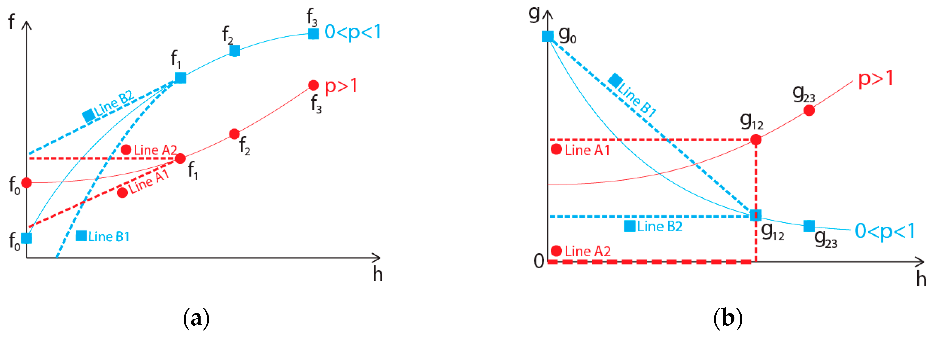
Based on GRE, if the solutions are within the asymptotic range, then the function of fh should be in the most part monotonic. There would be some wiggles in the data due to the HOT, but within the scale of f2 − f1, these HOT should be able to be ignored. The monotonic assumption would also apply to the derivative of fh which is denoted by g. Using this monotonic assumption as a basis, if 1 < p, then the limiting value of f0 could be modeled as Equation (6), with the value of g12 calculated with Equation (7). This modeling is possible since when p > 1, the value of |g(h ≤ h1)| would decrease as the cell size approaches zero. The limiting value of f0 is then taken by considering g(h ≤ h1) = g12 and g(h ≤ h1) = 0, in which upon integration resulted in Equation (6). This limiting value is also illustrated in Figure 2, in which line A1 represents the condition of g(h ≤ h1) = g12 and line A2 represents g(h ≤ h1) = 0.
Using the same approach, which is a gradient based analysis, the limiting values of f0 for the condition of 0 < p < 1 could also be obtained. One of these limiting value is g(h ≤ h1) = g12. As for the other limiting value, some additional modeling is required. This is due to |g(h ≤ h1)| in which it always increases as the cell size approaches zero. A quick glance would results in |g(h ≤ h1)|= ∞, which is unacceptable. As such, it is required to find an estimation of g0, so that the possible values of g(h ≤ h1) is limited.
After examining several datasets which satisfy the condition of 0 < p < 1, it is found that the inverse of the gradient (1/g) tends to behave linearly. Using this as a basis, Equation (9) is formed in which it shows how to calculate g0. A linear relationship with either h1, h2, or h3 is not done, since both g12 and g23 which is calculated by using Equations (7) and (8) are both estimates of the real gradient itself (e.g.,g12≠g1, g12≠g2). To ensure that the estimated g0would lead to a conservative estimate of f0, some modifications are needed, which in this case it is done by estimate of h which equal to g12 and g23, respectively (e.g., |gh12,min|≤| g12|≤| gh12,max|). These values are shown in Equations (10) and (11).
After obtaining the value of g0, the other limiting value of f0 could then be calculated, in which it occurs at g(h ≤ h1) = (g12+ g0)/2. This average form is taken due to its simplicity and robustness. Although as stated before that the inverse of the gradient tends to behave linearly, this model is not used as the value g0 is still considered as a guess. This could lead to some conservative issues, in which the model of g(h ≤ h1) = (g12+ g0)/2 is preferred as it is more conservative. Hence, the limiting values of f0for the condition of 0 < p < 1 is g(h ≤ h1) = g12 and g(h ≤ h1) = (g12 + g0)/2. Upon integration, it would result in Equation (12) and, respectively, shown in Figure 2 as line B2, and B1.
Some issues persist with Equations (6)–(12). Firstly, the estimate in the new model is discontinuous when p = 1. As some cases do tend to behave as p ≈ 1, this discontinues estimate could lead to some sensitivity issues. To alleviate the problem a safety factor was used so that the condition of where Equation (6) applies is set to 1.1 < p and for Equation (12) it only applies if 0 < p ≤ 1.1. Furthermore, to alleviate some concerns of the misinterpretation regarding the value of p due to its sensitivity, the condition of where Equation (6) applies is set to 1.1|g12| ≤ |g23|, and Equation (12) applies if 1.1|g12| > |g23|. For the sake of simplicity though, the condition of 1.1|g12| ≤ |g23| would be referred as condition A, and the condition of 1.1|g12| > |g23| would be referred as condition B.
For the second problem, when p ≈ 0, the estimation of g0becomes unrealistic. All gradients (g12, g23, and g0) should have the same sign, either positive or negative. A change in sign would suggest an oscillation in the simulated data (f), which breaks the basic assumption of this method. However, when the value of p is near 0, there is a tendency that the value of g0 would have a different sign from both g12 and g23. To alleviate this problem, Equation (13) is used.
Due to the difficulty in estimating a reliable estimate in the condition of p ≈ 0, within Equation (13), a wide estimate range is taken to ensure the conservativeness of such case. The value of −99f1 and 101f1 is taken to have the value of f1 to be the center of the estimate, and also it is considered to be less likely that the value of f0 would have a change of sign from the value of f1. Though there may not many useful practical usages from this equation, since the uncertainty is guaranteed to be 20000%, this equation is meant to evade any misleading estimate due to an unrealistic g0 value.
The third problem is the possibility if a mesh used for the simulation is not dense enough that it has a behavior of condition B, which upon refinement, changes to condition A. This leads to some conservative issues in Equation (12), which to ensure a conservative estimate, it is best to substitute the limiting value of f1 − g12h1 in Equation (12) with f1. The final problem is again in Equation (12), in which to ensure conservativeness, the variable of h1 should be substituted by h12max.
To summarize, the complete model of the suggested method is shown in Equations (4), (5), (14), and (15). The values of g12, g23, g0, h12max, and h23mn, are calculated using Equations (7)–(11), respectively. The definition of condition A is if 1.1|g12| ≤ |g23|and g0g12 >0, while the definition of condition B is 1.1|g12| > |g23|andg0g12 >0.
3. Evaluation Method
For the evaluation of the suggested method, a dataset of 11 different cases obtained by using the method of manufactured solution (MMS)[30] is prepared. From these cases, a total of 36 variables are taken for evaluation. For the detail of each case, the variables that are being evaluated, the number of mesh used for each case, and also the MMS equation; all of this could be seen in Table 1.
For each case in Table 1, it is simulated in one of two different applications which are also operated between two different computers. The application includes a self-coded python code in JetBrains PyCharm and Fluent. As for the computers, one is using an 8-core processor (Intel i5-8256U) with an 8 GB of RAM, and the other with a 24-core processor (AMD Threadripper 3960x) with a 32 GB of RAM. As each application is set on its default settings, the number of cores available for the calculation is 7 or 23 cores for JetBrains PyCharm and 1 core for Fluent.
To ensure the validity of the simulation, first the simulations are conducted by using a 64-bit floating number (double precision) to evade any interference from the round-off error [31] and simulated to machine accuracy limit to evade any potential iterative error. The result of this simulation is then compared to the MMS equation to ensure that it is indeed solving the right equation.
To be able to measure the time to simulate each mesh, the computer is set to safe mode to prevent any kind of interference, and also the simulation is conducted multiple times to ensure that the measured time is valid. Although the simulations are conducted on different programs and computers, for each case in Table 1, both of these factors would remain the same, thus it is possible to do a time comparison for each of the meshes in each case.
As some of the data obtained within this simulation do show oscillating behavior, some of the data are bound to be rejected. This rejection only occurs in the coarsest mesh of each simulation, indicating that those meshes are outside the asymptotic range. After rejection, on average, each variable would have data from 23 different meshes. As every non-oscillating triplet would be used for analysis, the number of triplets that is going to be used is 95,992 triplets.
There are three overall tests that are going to be conducted by accuracy, precision, and required computational time. The accuracy test measures how often the f0 estimate does contain the real f0 value. This could easily be done as the MMS method allows us to know the analytical solution of the simulation. The precision test is measuring how tight of an estimate is given by a method. This test is conducted by measuring how often the uncertainty or the GCI of a specific method is below a standard statistical acceptance of 10%, 5%, and 1%. For the computational time analysis, this measures the minimal real time that is needed for a computer to simulate three meshes, so that the data have an uncertainty below 10%, 5%, and 1%, if they are analyzed by a specific method. For the sake of convenience, the accuracy test is going to be measured by the conservativeness parameter defined in equation 16, with the value of f0,guess = f1 and U = GCI for the GCI method. As for the precision test, this is going to be measured by a probability parameter shown in equation 17, with UTarget is set to 10%, 5%, and 1%. All of these tests are going to be conducted with the gradient based method, Roache’s method, and also some improvement of Roache’s method which is proposed by Oberkampf and Roy [16], Stern-Wilson [19,21], and Xing and Stern [22]. Each of these methods will be denoted as Ugradient, GCIR, GCIOR, GCISW, and GCIXS.
4. Results
For the result of the accuracy test, the value of Ψ can be seen in Table 2. There are three different values of Ψ in this analysis, which aim to minimize the effect of any possible kind of bias within the analysis, for example due to the different number of data points on each case. For ΨOverall, this is the value of Ψ from all of the 95,922 triplets. For ΨCase, this is the average value of Ψ on every case. For Ψp, this is the averaged value of Ψ from a group of 31 intervals of p, each with an interval of 0.1 in the range of 0 < p ≤ 3 and a separate individual group for 3 < p.
From the result of the accuracy analysis it could be seen that for every variation of Ψ, the value of Ψ from Ugradient is the highest of them all. This consistent result across all variation of Ψ, shows that the gradient-based method does indeed perform better than all the other methods. This means that even though the gradient-based method uses the value of f0,guess as the center of the estimate, as the model is built upon this assumption, the accuracy is not affected at all, and this method manages to estimate the value of f0 better than the other methods.
To understand where each method failed, the failure rate of each method based on its p value is shown in Figure 3. In general, the failures could be divided into three parts, which are 0 < p ≤ 1, 1 < p ≤ 2, 2 < p. For the range of 0 < p ≤ 1, the failure could only be seen for Ugradient. This failure is due to the estimation of g0 which is sometimes not conservative enough. For the range of 2 < p, the failures are mainly caused by triplets that include data from some very coarse mesh with have a behavior that is different from the rest. These data might as well be considered outside the asymptotic range, thus by including them in the analysis, they are expected to produce a high failure rate. The other source of failure only applies to GCIR, in which it could be seen that in this range, the failure rate is significantly higher than the other methods. The cause of this failure is due to the value of p that exceeds the formal order of accuracy (pf) which is usually 1 or 2. This would cause the value of GCI to be very small but it tends to be less accurate. This is an already known problem for GCIR, in which the other variations of GCI have tried to prevent. As such, they tend to have a lower failure rate.
As for the range of 1 < p ≤ 2, for GCIR, the failures are caused by the same reasons as the failures for the range of 2 < p, which are some coarse meshes that behaves differently and also a p value that exceeds the value of pf. This is possible since the failure at the range of 2 < p has the properties of pf = 2. However, within the range 1 < p ≤ 2, the failures are caused by the data that have the properties of pf = 1. As such the same reason of failures applies, although there are some differences that need to be addressed. First, within the data with pf = 2 there are some data with the p value lower than what tends to be accurate. This would have an effect of the failures in the range of 1 < p ≤ 2, which is not as significant as the failures in the range of 2 < p. Second, is that for the data with a p value that exceeds pf = 1, the deviation is usually not that far off. As such the value of p is found to be limited to p < 2. This caused a drastic reduction in failure rate from 1 < p ≤ 2 to 2 < p ≤ 2.2. As for the variations of GCIR, the same reasons also apply. However, as each method has tried to improve upon GCIR, the failures are usually less than GCIR with a varying degree of success.
For Ugradient, within the same range of 1 < p ≤ 2,the failures are caused mainly by a wrong usage of the equation for condition A, in which the data do mathematically fit the description of condition A, although the overall trend shows that condition B should actually be applied. With the boundary between condition A and B is around 1.1, this caused the failures to be focused around this value and above it. As such, a high failure rate is not observed for 1 < p, but the failure rate is not only focused on 1 < p ≤ 1.2, but also spreads to 1 < p < 1.6. However, it should be known that the misinterpretation of the conditions is more likely to occur near p = 1. As such the failure rate would decrease on a higher value of p.
For the precision test, this result is shown in Table 3. It could be seen that there are again 3 variations of Γ, which is again to minimize any possible bias. These variations have a similar definition as the Ψ variations in the accuracy test. It should be known that the data in Table 3 are required to be conservative, since if the data are not conservative, regardless if the uncertainty is high or low, it would be meaningless if it is not accurate. From all of these variations, there are two things that have to be considered. First is that the value of Γ would be higher for a higher UTarget. This is obvious since a tighter estimate would be harder to obtain, thus the value of Γ would be lower. The second one is that it could be once again seen that Ugradient has the highest Γ, which indicates that this method does tend to produce the tightest estimate of f0, or the lowest uncertainty of the f0 estimate. This is again caused by design, as the gradient based method uses the value of f0,guess to be the center of the estimate, thus allowing for a lower uncertainty.
As for the time analysis, this result is shown in Table 4, in which it is showing the average time saving of each method compared to GCIR. The positive sign in this data shows that the method does on average requires less real time to simulate a certain case, and a negative sign means that the method, on average requires more real time for its simulation. It should be known that once again, the data used for this analysis must be conservative.
In Table 4, it could be seen that Ugradient is the only method that manage to reduce the required computational time, in which it is reduced by 15%–30%. It should be known that this is the averaged value. There are cases where the other methods also save time, and there are cases where Ugradient requires more time. Some example of the time required to simulate a case, and obtain an acceptable uncertainty is shown in Table 5.
The general reason why Ugradient manages to save time is due to the possibility of the method to analyze data from a more coarse mesh, and does produce an accurate and precise estimate. This is a very big advantage, as the computational time would increase significantly as the mesh is gets denser. As such, even by just evading one more mesh refinement, there could be a significant time saving.
Observing the data, it seems that the saving would be much more significant if the overall data is on condition B. Some examples of the cases that fits this condition is shown in Figure 4, in which for case 24 itself, the time saving for this case is 50.15%, 50.15%, and 90.32%, respectively, for UTarget = 10%, 5%, and 1%. On the other hand, if the data are in condition A, especially if the data are parabolic (p ≈ 2), the time saving would be less significant, even there might not be any time saving at all. The examples of the cases that fit this condition are shown in Figure 5, where the most extreme example is case 3 which has a time saving of −13.63%, −31.78%, and −35.65%, respectively, for UTarget = 10%, 5%, and 1%. The cause of this difference is apparently due to precision issues.
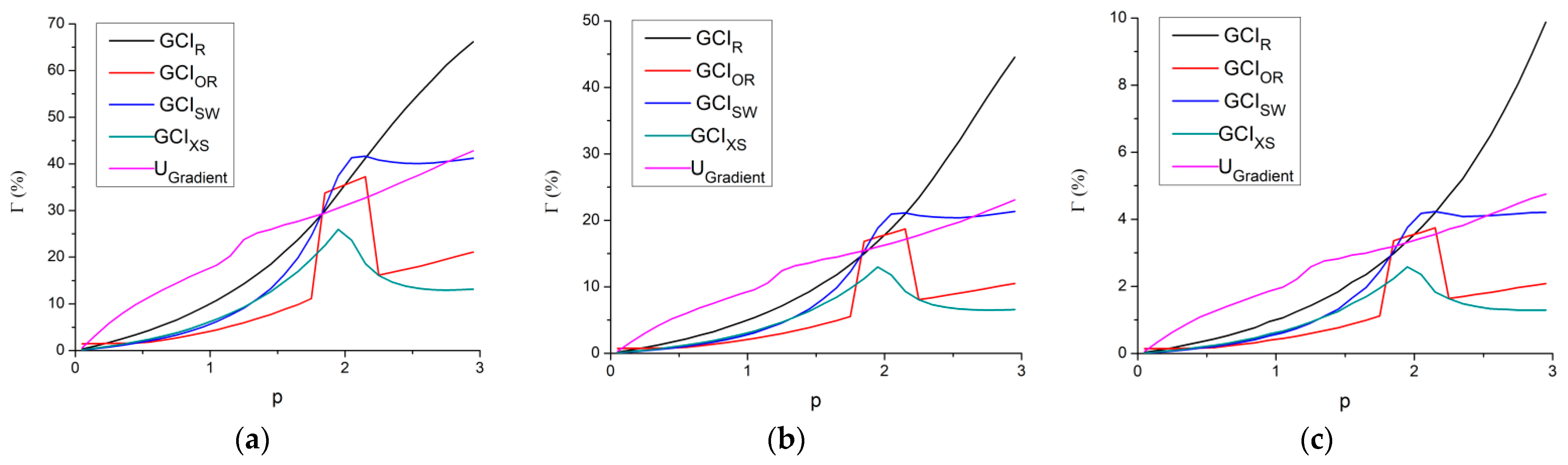
Although previously it has been shown that the Ugradient gave the tightest estimate, or it is the more precise method, this is not true across all conditions. On a higher value of p, the other methods tend to be better than Ugradient if the accuracy issue is ignored. To prove this, the precision test would be conducted once again, but this time the dataset would consist of multiple random values of p, r12, r23, and also f3/f1. The interval of p is set to be 0 < p ≤ 3, while all the other variables is set to 1 < r12, r23, f3/f1 ≤ 2. A total of 3 × 10⁷ random data are taken and the Γ value is calculated once again. This result which is shown in Figure 6 shows that upon 1.8< p, some other methods tend to be equal or even better than Ugradient. This is especially true for GCIR. A word of caution though, as these data do not take the accuracy into consideration. As seen in Figure 3, that especially for GCIR with 2.2 < p, the failure is already very significant, that it could not be recommended for normal usage.
The effect of this result in the time analysis is that even if 2.2 < p, since there is a lot of combination on each case, there would be at least 1 triplet that is conservative. As such, these data are used for the time analysis. This would result in GCIR to have the lowest uncertainty estimate, thus this method could utilize a more coarse mesh to obtain an uncertainty equal or below UTarget and the overall time would be lower than all the other methods.
Considering Figure 3 and Figure 6, for 1.8 < p, where there are several methods that perform better in terms of accuracy than Ugradient and do not have a low failure rate; there is a chance that these methods do have a lower computational time than Ugradient. This suggests that the usage of Ugradient to save time would be more significant if the data has a value of p < 1.8. This trend apparently occurs quite often in our dataset, especially when the meshes are coarse enough. However, upon refinement, there is a tendency that the data would behave as p ≈ 2 which have a minimal time saving. This switch in behavior is one of the cause that the time saving for Ugradient at UTarget = 1% is lower compared to the rest. Some examples of the cases with switching behavior are shown in Figure 7, in which for case 35 itself, the time savings are 15.86%, 38%, and −47.43%, for, respectively, UTarget = 10%, 5%, and 1%. All of this suggests that the usage of Ugradient is much better aimed at coarse meshes, with p < 1.8.
Judging by the data from Table 4, in which the data on this table show the averaged time saving from all across the p spectrum, it could be inferred that for data with p < 1.8, then the time saving should be higher. As such, as engineers usually use a 5% uncertainty, then for a simulation data with p < 1.8, the time saving by using Ugradien compared to GCIR is on average at least 25%. This is a significant amount of time saving and it could potentially be more. The maximum time saving that is observed in this dataset is up to 89.22%, which occurs in case 1 for UTarget = 5%.
5. Study Case
To show the performance of the gradient based method on a real simulation, a study case would be presented. A simulation of an air flow passing through a 100 mm diameter cylinder is conducted. This flow is single phased, and have a uniform velocity distribution of 5 m/s, in which overall it correlates to a Reynolds number of 34,300. A total of 16 meshes are going to be used ranging from 1536 cells to 230,496 cells, of which the cell distribution is shown in Figure 8 and for each mesh the mesh is refined in a systematic manner. The simulation is solved in a steady-state manner using a standard k-ε turbulence model with a near wall formulation is used for the cells near the wall. For the discretization, it is done by using a finite volume method with a second order accurate method is used to interpolate the face values. The simulation is then iterated until it reaches machine accuracy, in which then the drag coefficient (CD) could be obtained.
The result of this simulation could be seen in Figure 9. First it could be seen that the data do behave monotonically and no oscillation is observed. This means that every triplet in this simulation could be calculated using the GCI and the gradient-based method. Although the accuracy test could not be done for these data since the analytical solution of this case is unknown, the precision test and the required computational time could still be done. Both of these test results are shown, respectively, in Table 6 and Table 7.
The data on Table 6 and Table 7 have the same tendencies as the result from the MMS simulations. The value of the Γ from Ugradient tends to be always the highest, which means that Ugradient is the most precise method. This precision also translates to the required computational time, in which for UTarget = 5%, it saves 50.17% over GCIR and for UTarget = 1%, it saves 51.51%. There is no time saving in UTarget = 10% since all the uncertainties from both GCIR and Ugradient even from the coarsest mesh is already below 10%. This does show that the result on the MMS simulation could also apply into a real engineering case simulation.
Regarding the application of Ugradient to a real engineering case, it should be noted that within this example, this is a simple case where there is a single phase flow that passes through a simple geometry at a rather low Reynolds number of 34,300. This is much simpler case than any kind of real world application of CFD. At a higher complexity, or higher Reynolds number flow, it is expected that the data tend to oscillates more, thus making it incompatible with the GCI and Ugradient. This would require some mesh refinement, in which sometimes, to make sure the data do not oscillate, the required mesh is not practical to be created or even simulated. This does limit the application of both GCI and Ugradient. However, with the advantages that Ugradient have, the required mesh is only required to not oscillate any more. If the mesh does not oscillate any more, which means that Ugradient can be applied, it has been shown that Ugradient could produce an accurate and precise estimate even from coarse meshes. For comparison the GCIR would require the mesh to not only stop oscillating but also be well behaved (p≈pf) to ensure that the estimate is both accurate and precise.
6. Conclusions
In this study, a new method to estimate a discretization error in CFD is presented. The method is based on the behavior of the gradient in a CFD simulation result. This method is tested on an MMS simulation dataset, in which the results show that even by changing the center of estimation from f1 to f0,guess, the gradient-based method can still estimate the value of f0 even to a degree that is more accurate than the other method tested in this study. This gradient-based method is also shown to be more precise, especially for p < 1.8, which usually occurs on coarser meshes. This higher precision is a significant advantage for the gradient based method since it does allow the usage of a coarser mesh to obtain a certain level of uncertainty, thus reducing the overall computational time required for the simulation. For the range that this method is recommended for, which is p < 1.8, the time saving is compared to the standard GCI with a targeted uncertainty of 5%, is on average at least 25%. This significant advantage would be useful for analyzing CFD simulation results.
The standard GCI is only practical for a low Reynolds number flow. However, with the advantage that the gradient-based method has, it might be practical up to a medium Reynolds number flow. It is not sure that this method would be suitable for a high Reynolds flow simulation or a more complex simulation, since the result of such simulation usually has a high tendency to oscillate which does break the assumptions of the gradient-based method.
Although it might not be perfect, nor it is applicable to every CFD simulation, the gradient-based method that has been shown is capable of performing better than the standard GCI. It is more accurate, more precise, and may reduce the overall computational time by a significant amount. As such, we do recommend the use of this method for analyzing the results of CFD.
Author Contributions
Conceptualization, A.S.; methodology, A.S.; software, A.S.; validation, A.S.; formal analysis, A.S.; writing—original draft preparation, A.S.; writing—review and editing, A.S.; visualization, A.S.; supervision, H.; project administration, H.; funding acquisition, A.S. and H. All authors have read and agreed to the published version of the manuscript.
Funding
This research was funded by Universitas Indonesia in PUTI Q2 2020, grant number NKB-1712/UN2.RST/HKP05.00/2020.
Institutional Review Board Statement
Not applicable
Informed Consent Statement
Not applicable.
Data Availability Statement
Data sharing is not applicable to this article.
Conflicts of Interest
The authors declare no conflict of interest. The funders had no role in the design of the study; in the collection, analyses, or interpretation of data; in the writing of the manuscript, or in the decision to publish the results.
Abbreviation
| ASME | The American Society of Mechanical Engineers |
| AIAA | American Institute of Aeronautics and Astronautics |
| CFD | Computational fluid dynamics |
| GCI | Grid convergence index |
| GRE | Generalized Richardson extrapolation |
| MMS | Method of manufactured solutions |
Nomenclature
| a,b | Constants | HOT | Higher Order Terms |
| CD | Drag Coefficient | µ | Viscosity |
| f0 | Analytical result | p | Order of convergence |
| f0,guess | Guessed analytical result | pf | Formal order of accuracy |
| fh | Simulation result of mesh with cell size h | P | Pressure |
| f1,2,3 | Simulation result of mesh index 1,2, or 3 | Ψ | Conservativeness |
| g0 | Gradient at cell size = 0 | rab | Cell size ratio of mesh index a and b |
| ga | Gradient at mesh index a | SF | Safety Factor |
| gab | Gradient of mesh index a and b | t | Time |
| GCI | Grid Convergence Index | T | Temperature |
| Γ | Probability of U or GCI ≤ UTarget | τ | Shear Stress |
| ha | Cell size of mesh index a | u,v,w | Velocity |
| h12max | Maximum possible h value that has a gradient equal to g12 | U | Uncertainty |
| h23min | Minimum possible h value that has a gradient equal to g23 | UTarget | Targeted uncertainty value |
References
- Roy, C.J. Grid Convergence Error Analysis for Mixed-Order Numerical Schemes. AIAA J. 2003, 41, 595–604. [Google Scholar] [CrossRef] [Green Version]
- ASME Committee V&V 20. Standard for Verification and Validation on Computational Fluid Dynamics and Heat Transfer; The American Society of Mechanical Engineers: New York, NY, USA, 2009. [Google Scholar]
- American Institute of Aeronautics and Astronautics (AIAA). Guide for the Verification and Validation of Computational Fluid Dynamics Simulations; American Institute of Aeronautics and Astronautics: Reston, VA, USA, 2002. [Google Scholar]
- Roache, P.J. Verification of Codes and Calculations. AIAA J. 1998, 36, 696–702. [Google Scholar] [CrossRef]
- Rider, W.; Witkowski, W.; Kamm, J.R.; Wildey, T. Robust verification analysis. J. Comput. Phys. 2016, 307, 146–163. [Google Scholar] [CrossRef] [Green Version]
- Roy, C.J. Review of code and solution verification procedures for computational simulation. J. Comput. Phys. 2005, 205, 131–156. [Google Scholar] [CrossRef]
- Oberkampf, W.L.; Trucano, T.G. Verification and validation in computational fluid dynamics. Prog. Aerosp. Sci. 2002, 38, 209–272. [Google Scholar] [CrossRef] [Green Version]
- Roache, P.J. Verification and Validation in Computational Science and Engineering, 1st ed.; Hermosa Publishers: Albuquerque, NM, USA, 1998. [Google Scholar]
- Roy, C.J.; Oberkampf, W.L. A comprehensive framework for verification, validation, and uncertainty quantification in scientific computing. Comput. Methods Appl. Mech. Eng. 2011, 200, 2131–2144. [Google Scholar] [CrossRef]
- Roy, C.J. Review of Discretization Error Estimators in Scientific Computing. AIAA Pap. 2010, 2010–2126. [Google Scholar] [CrossRef]
- Roache, P.J. Perspective: A Method for Uniform Reporting of Grid Refinement Studies. J. Fluids Eng. 1994, 116, 405–413. [Google Scholar] [CrossRef]
- Celik, I.B.; Ghia, U.; Roache, P.J.; Freitas, C.J. Procedure for estimation and reporting of uncertainty due to discretization in CFD applications. J. Fluids Eng. 2008, 130:078001. [Google Scholar]
- American Institute of Aeronautics and Astronautics (AIAA). Editorial Policy Statement on Numerical and Experimental Accuracy. AIAA J. 2013, 51. [Google Scholar] [CrossRef]
- Richardson, L.F. The Approximate Arithmetical Solution by Finite Differences of Physical Problems Involving Differential Equations, with an Application to the Stresses in a Masonry Dam. Phil. Trans. R. Soc. Lond. A 1911, 210, 307–357. [Google Scholar]
- Richardson, L.F. The Deferred Approach to the Limit. Part I. Single Lattice. Phil. Trans. R. Soc. Lond. A 1927, 226, 299–349. [Google Scholar]
- Oberkampf, W.L.; Roy, C.J. Verification and Validation in Scientific Computing; Cambridge University Press: Cambridge, UK, 2010. [Google Scholar]
- Eca, L.; Hoekstra, M. An Evaluation of Verification Procedures for CFD Applications. In Proceedings of the 24th Symposium on Naval Hydrodynamics, Fukuoka, Japan, 8–13 July 2002. [Google Scholar]
- Eca, L.; Vaz, G.; Hoekstra, M. A contribution for the Assessment of Discretization Error Estimators Based on Grid Refinement Studies. J. Verif. Valid. Uncertain. Quantif. 2018, 3, 021001. [Google Scholar] [CrossRef]
- Stern, F.; Wilson, R.V.; Coleman, H.W.; Paterson, E.G. Comprehensive Approach to Verification and Validation of CFD Simulations — Part 1: Methodology and Procedures. J. Fluids Eng. 2001, 123, 793–802. [Google Scholar] [CrossRef]
- Cadafalch, J.; Segarra-Perez, C.D.; Consul, R.; Oliva, A. Verification of Finite Volume Computations on Steady-State Fluid Flow and Heat Transfer. J. Fluids Eng. 2002, 124, 11–21. [Google Scholar] [CrossRef]
- Wilson, R.V.; Shao, J.; Stern, F. Discussion: Criticisms of the ‘Correction Factor’ Verification Method. J. Fluids Eng. 2004, 126, 704–706. [Google Scholar] [CrossRef]
- Xing, T.; Stren., F. Factors of Safety for Richardson Extrapolation. J. Fluids Eng. 2010, 132, 061403. [Google Scholar] [CrossRef] [Green Version]
- Eca, L.; Hoekstra, M. A procedure for the estimation of the numerical uncertainty of CFD calculations based on grid refinement studies. J. Fluids Eng. 2014, 262, 104–130. [Google Scholar]
- Phillips, T.S.; Roy, C.J. A New Extrapolation-Based Uncertainty Estimator for Computational Fluid Dynamics. J. Fluids Eng. 2016, 1, 041006. [Google Scholar] [CrossRef]
- Phillips, T.S.; Roy, C.J. Evaluation of Extrapolation-Based Discretization Error and Uncertainty Estimators. AIAA Pap. 2011. [Google Scholar] [CrossRef]
- Celik, I.B.; Parons, D.R., III. Prediction of discretization error using the error transport equation. J. Comput. Phys. 2017, 339, 96–125. [Google Scholar] [CrossRef] [Green Version]
- Yan, G.K.; Ollivier-Gooch, C. On Efficiently Obtaining Higher Order Accurate Discretization Error Estimates for Unstructured Finite Volume Methods Using the Error Transport Equation. J. Verif., Valid. Uncertain. Quantif. 2017, 2, 041003. [Google Scholar] [CrossRef]
- Wang, H.; Tyson, W.C.; Roy, C.J. Discretization Error Estimation for Discontinuous Galerkin Methods using Error Transport Equations. AIAA Pap. 2019. [Google Scholar] [CrossRef]
- Roache, P.J. Quantification of Uncertainty in Computational Fluid Dynamics. Annu. Rev. Fluid. Mech. 1997, 29, 123–160. [Google Scholar] [CrossRef] [Green Version]
- Roache, P.J. Code Verification by the Method of Manufactured Solutions. J. Fluids Eng. 2002, 124, 4–10. [Google Scholar] [CrossRef]
- Eca, L.; Vas, G.; Toxopeus, S.L.; Hoekstra, M. Numerical Errors in Unsteady Flow Simulations. J. Verif. Valid. Uncertain. Quantif. 2019, 4, 021001. [Google Scholar] [CrossRef]
Figure 1.
An illustration of how uncertainty is calculated: (a) within computational fluid dynamics (CFD); (b) within an experiment.
Figure 1.
An illustration of how uncertainty is calculated: (a) within computational fluid dynamics (CFD); (b) within an experiment.

Figure 2.
A visual representation of how the limiting value is calculated with the suggested model: (a) on the simulation data; (b) on the gradient.
Figure 2.
A visual representation of how the limiting value is calculated with the suggested model: (a) on the simulation data; (b) on the gradient.

Figure 3.
Failure rate of each method, based on the value of p.

Figure 4.
The MMS simulation result that fits condition B: (a) Case 12; (b) Case 24; (c) Case 30.

Figure 5.
The MMS simulation result that fits condition A: (a) Case 3; (b) Case 6; (c) Case 32.

Figure 6.
The result of a random data test: (a) UTarget = 10%; (b) UTarget = 5%; (c) UTarget = 1%.

Figure 7.
The MMS simulation result that has switching conditions: (a) Case 20; (b) Case 35.

Figure 8.
The cell distribution in the simulation of a flow passes through a cylinder.

Figure 9.
The simulation result of a flow passes through a cylinder: (a) CD; (b) time.


Table 1.
Details of the method of manufactured solution (MMS) simulations.
| No | Case | Variable | Total Mesh | MMS Equation |
|---|---|---|---|---|
| 1 | 1D Heat Equation (First and Second order accurate) | T | 26 | |
| 2 | 35 | |||
| 3 | Laplace Equation | 25 | ||
| 4 | 1D Convection+ Difusion Equation | T | 44 | |
| 5 | Hagen–Poiseuille (First and Second order accurate)(Uniform Mesh) | 32 | ||
| 6 | ||||
| 7 | ||||
| 8 | ||||
| 9 | ||||
| 10 | ||||
| 11 | Hagen–Poiseuille (Non-Uniform Mesh) | 21 | ||
| 12 | ||||
| 13 | ||||
| 14 | Modified Hagen–Poiseuille— piecewise x-velocity | 30 | ||
| 15 | ||||
| 16 | ||||
| 17 | ||||
| 18 | ||||
| 19 | Annulus Flow | 19 | ||
| 20 | ||||
| 21 | ||||
| 22 | ||||
| 23 | Boundary Layer | 32 | ||
| 24 | ||||
| 25 | ||||
| 26 | ||||
| 27 | Diffuser | 17 | ||
| 28 | ||||
| 29 | ||||
| 30 | ||||
| 31 | ||||
| 32 | Nozzle | 25 | ||
| 33 | ||||
| 34 | ||||
| 35 | Cavity Flow | 28 | ||
| 36 |
Table 2.
Result of the Accuracy Test.
| Method | ΨOverall | ΨCase | Ψp |
|---|---|---|---|
| GCIR | 90.49% | 87.27% | 81.11% |
| GCIOR | 96.95% | 96.13% | 91.84% |
| GCISW | 96.11% | 94.68% | 90.16% |
| GCIXS | 97.85% | 95.05% | 91.92% |
| Ugradient | 98.94% | 96.75% | 92.56% |
Table 3.
Result of the Precision Test.
| UTarget(%) | Method | ΓOverall | ΓCase | Γp |
|---|---|---|---|---|
| GCIR | 76.29% | 60.46% | 57.04% | |
| GCIOR | 76.74% | 63.37% | 59.08% | |
| 10% | GCISW | 78.56% | 61.98% | 59.67% |
| GCIXS | 78.94% | 62.02% | 59.47% | |
| Ugradient | 84.76% | 67.59% | 66.82% | |
| GCIR | 72.61% | 56.29% | 52.39% | |
| GCIOR | 72.35% | 57.72% | 53.04% | |
| 5% | GCISW | 74.36% | 57.68% | 54.66% |
| GCIXS | 73.82% | 56.54% | 52.64% | |
| Ugradient | 82.02% | 64.42% | 62.58% | |
| GCIR | 58.82% | 43.39% | 37.85% | |
| GCIOR | 50.85% | 38.35% | 21.35% | |
| 1% | GCISW | 55.46% | 40.92% | 34.47% |
| GCIXS | 53.18% | 39.16% | 22.70% | |
| Ugradient | 67.35% | 50.66% | 44.11% |
Table 4.
Average Computational Time Saving Compared to Roache’s Method.
| Method | UTarget = 10% | UTarget = 5% | UTarget = 1% |
|---|---|---|---|
| GCIR | 0% | 0% | 0% |
| GCIOR | −182.86% | −76.39% | −84.42% |
| GCISW | −24.61% | −17.12% | −44.45% |
| GCIXS | −138.40% | −107.16% | −165.81% |
| Ugradient | 26.23% | 27.76% | 14.83% |
Table 5.
Several Examples of Required Simulation Time.
| Method | Time (s) | |||
|---|---|---|---|---|
| Case 10 (UTarget = 10%) | Case 20 (UTarget = 5%) | Case 24 (UTarget = 1%) | Case 35 (UTarget = 1%) | |
| GCIR | 47.646 | 3594.817 | 5522.303 | 17,708.15 |
| GCIOR | 51.846 | 3523.34 | 15333.32 | 30,509.99 |
| GCISW | 50.591 | 3523.34 | 15333.32 | 24,218.85 |
| GCIXS | 50.591 | 6464.425 | 5564.398 | 50,600.98 |
| Ugradient | 44.878 | 674.898 | 534.6054 | 26,107.87 |
Table 6.
The precision test result of the simulation of a flow passes through a cylinder.
| Method | Γ | ||
|---|---|---|---|
| UTarget = 10% | UTarget = 5% | UTarget = 1% | |
| GCIR | 100.00% | 98.35% | 38.74% |
| GCIOR | 96.98% | 70.88% | 0.82% |
| GCISW | 100.00% | 95.05% | 16.48% |
| GCIXS | 100.00% | 93.68% | 18.41% |
| Ugradient | 100.00% | 100.00% | 55.77% |
Table 7.
The required computational time of the simulation of a flow passes through a cylinder.
| Method | Time (s) | ||
|---|---|---|---|
| UTarget = 10% | UTarget = 5% | UTarget = 1% | |
| GCIR | 765.964 | 1537.095 | 40,103.05 |
| GCIOR | 1983.451 | 3161.402 | 45,013.19 |
| GCISW | 765.964 | 1993.79 | 41,529.36 |
| GCIXS | 765.964 | 1993.79 | 75,110.02 |
| Ugradient | 765.964 | 765.964 | 19,444.85 |
Publisher’s Note: MDPI stays neutral with regard to jurisdictional claims in published maps and institutional affiliations. |
© 2021 by the authors. Licensee MDPI, Basel, Switzerland. This article is an open access article distributed under the terms and conditions of the Creative Commons Attribution (CC BY) license (http://creativecommons.org/licenses/by/4.0/).
Share and Cite
MDPI and ACS Style
Satyadharma, A.; Harinaldi. The Performance of a Gradient-Based Method to Estimate the Discretization Error in Computational Fluid Dynamics. Computation 2021, 9, 10. https://0-doi-org.brum.beds.ac.uk/10.3390/computation9020010
AMA Style
Satyadharma A, Harinaldi. The Performance of a Gradient-Based Method to Estimate the Discretization Error in Computational Fluid Dynamics. Computation. 2021; 9(2):10. https://0-doi-org.brum.beds.ac.uk/10.3390/computation9020010
Chicago/Turabian StyleSatyadharma, Adhika, and Harinaldi. 2021. "The Performance of a Gradient-Based Method to Estimate the Discretization Error in Computational Fluid Dynamics" Computation 9, no. 2: 10. https://0-doi-org.brum.beds.ac.uk/10.3390/computation9020010
Note that from the first issue of 2016, this journal uses article numbers instead of page numbers. See further details here.