Kinetic Simulations of Compressible Non-Ideal Fluids: From Supercritical Flows to Phase-Change and Exotic Behavior

Abstract

We investigate a kinetic model for compressible non-ideal fluids. The model imposes the local thermodynamic pressure through a rescaling of the particle’s velocities, which accounts for both long- and short-range effects and hence full thermodynamic consistency. The model is fully Galilean invariant and treats mass, momentum, and energy as local conservation laws. The analysis and derivation of the hydrodynamic limit is followed by the assessment of accuracy and robustness through benchmark simulations ranging from the Joule–Thompson effect to a phase-change and high-speed flows. In particular, we show the direct simulation of the inversion line of a van der Waals gas followed by simulations of phase-change such as the one-dimensional evaporation of a saturated liquid, nucleate, and film boiling and eventually, we investigate the stability of a perturbed strong shock front in two different fluid mediums. In all of the cases, we find excellent agreement with the corresponding theoretical analysis and experimental correlations. We show that our model can operate in the entire phase diagram, including super- as well as sub-critical regimes and inherently captures phase-change phenomena.

1. Introduction

The lattice Boltzmann method (LBM) is a kinetic-theory approach to the simulation of hydrodynamic phenomena with applications ranging from turbulence [1,2] to microflows [3,4] and multiphase flows [5,6,7,8]. The fully discretized kinetic equations evolve particle distribution functions (populations) $f_i(\mathit{x},t)$, which are associated with a set of discrete velocities ${\mathit{c}}_i$, according to a simple stream-and-collide algorithm and recover the Navier–Stokes equations in the hydrodynamic limit [9].

While LBM has proven successful in a wide range of fluid mechanics problems [9,10], it is well known that the fixed velocity set restricts conventional LB models to low-speed incompressible flows [9]. This promoted significant research efforts, which were directed towards the development of compressible LB models [11,12,13,14,15], but they are typically limited to ideal gas. A genuine LB model, which can capture both compressible and non-ideal fluids has been lacking. However, in many scientific and engineering applications the ideal-gas assumption is no longer valid and real-gas effects have to be taken into account. This includes phenomena such as rarefaction shock waves [16,17,18,19], acoustic emission instability [20,21], inversion line (change of sign of the Joule–Thomson coefficient), phase transition, surface tension, and super-critical flows.

While LB models for non-ideal gases have been subject to many studies in the literature, they are mostly restricted to incompressible flows. In the incompressible regime, two main approaches for non-ideal gases exist: Pressure-based methods [22,23] and forcing methods [24,25,26,27]. Pressure-based methods were pioneered by Swift et al. [22] and alter the equilibrium populations such that the full non-ideal pressure tensor, including the non-ideal equation of state (EOS) and the Korteweg stress, are recovered. However, it was soon realized that these methods are not Galilean invariant [23,27,28] and lack thermodynamic consistency [29]. Although various improvements have been proposed in the literature (see, e.g., [23,27,28,30]) their range of validity and stability remains limited [27]. On the other hand, forcing methods account for the deviation from the ideal-gas pressure by an appropriate (non-local) force term, which is introduced in the kinetic equations. Forcing methods are generally more stable than the pressure-based methods and the Galilean invariance error can be reduced effectively if augmented with appropriate correction terms [27]. Promising results have been obtained for forcing methods in various of applications, ranging from droplet collisions at relatively large density ratios [31,32] to droplet impact on textured [33] and flexible surfaces [34].

The aforementioned models have also been extended to thermal multiphase flows, including phase change. For instance, a common approach is to solve the temperature equation by conventional finite difference or finite volume schemes, which is then coupled to the flow field by a non-ideal EOS. As shown in [35,36], one can capture nucleate, transient, and film boiling. Another common approach is to use a second set of population for the temperature equation, which is combined with additional source terms to account for phase change [37,38,39]. Under the low Mach conditions, these methods are commonly associated with simplifying assumptions such as neglecting the viscous heat dissipation [39] or the pressure work [38,40] which lead to a tailored form of the energy equation. Therefore, these models are not able to capture high-speed compressible flow of non-ideal fluids, where a complex temperature field with a wide range of values is expected to emerge.

To mitigate these shortcomings, we recently proposed a novel method for non-ideal compressible fluid dynamics [41] based on adaptive discrete velocities in accordance to local flow conditions. In contrast to the aforementioned schemes, the model features full Galilean-invariance and is thermodynamically consistent. As a consequence of the model’s construction, the full energy-equation of a non-ideal fluid is recovered, which means that no additional phase-change model is required. This enables us to capture a large range of flow regimes, which we aim to explore in this paper. While basic validation was conducted in [41], we extend this analysis here and assess the model’s performance for super-critical flows, throttling, phase change, and shock-stability.

The paper is structured as follows: Section 2 provides an in-depth analysis of the model. We start with a presentation of the discrete kinetic equations in Section 2.1, followed by the Chapman–Enskog analysis and the derivation of the hydrodynamic limit in Section 3. Numerical benchmarks including the simulation of the Joule–Thomson effect, phase-change, and high-speed flows are presented in Section 4. Finally, conclusions are drawn in Section 5.

2. Methodology

2.1. Kinetic Equations

Our thermokinetic model of non-ideal fluids [41] is based on the so-called particles-on-demand (PonD) method [13], which constructs the particle’s velocities relative to the reference frame (gauge) $\lambda =\{T,\mathit{u}\}$, where T is the local temperature and $\mathit{u}$ is the local flow velocity. While the former leads to thermodynamic consistency, the latter guarantees Galilean invariance. In addition, in the local reference frame, the local equilibrium becomes exact and solely dependent on the density. This is in contrast to classical LBM where one typically resorts to a truncated polynomial. The populations can be transformed between different reference frames by requiring the moments to be independent of the reference frame [13]. In [41], we generalized this concept to encompass the thermodynamics of non-ideal fluids by defining the new set of discrete velocities as:

$${\mathit{v}}_i=\sqrt{\frac{p}{\rho T_{\mathrm{L}}}}{\mathit{c}}_i+\mathit{u},$$

(1)

where $p(\mathit{x},t)$ is the local thermodynamic pressure, $\rho (\mathit{x},t)$ is the local density, and $T_{\mathrm{L}}$ is a lattice reference temperature, a constant known for any set of speeds $\mathcal{C}=\{{\mathit{c}}_i,i=1,...,Q\}$, and $\mathit{u}(\mathit{x},t)$ is the local flow velocity.

A two-population approach is employed in this study. While f populations maintain the density and the momentum field, the g populations carry the total energy. As in classical LBM, a stream and collide algorithm is used to evolve the populations in time. In particular, we use a semi-Lagrangian approach for advection along the characteristics [42,43] at the monitoring point $(\mathit{x},t)$, which reads:

$$\begin{array}{ccc}\hfill f_i^{\lambda }(\mathit{x},t)& =& {\widetilde{f_i}}^{\lambda }(\mathit{x}-{\mathit{v}}_i\delta t,t-\delta t),\hfill \end{array}$$

(2)

$$\begin{array}{ccc}\hfill g_i^{\lambda }(\mathit{x},t)& =& {\widetilde{g_i}}^{\lambda }(\mathit{x}-{\mathit{v}}_i\delta t,t-\delta t),\hfill \end{array}$$

(3)

while the Bhatnagar–Gross–Krook (BGK) model is employed for the collision step:

$$\begin{array}{ccc}\hfill f_i(\mathit{x},t)& =& f_i^{\lambda }(\mathit{x},t)+\omega (f_i^{\mathrm{eq}}-f_i^{\lambda }(\mathit{x},t))+S_i^{\lambda },\hfill \end{array}$$

(4)

$$\begin{array}{ccc}\hfill g_i(\mathit{x},t)& =& g_i^{\lambda }(\mathit{x},t)+\omega (g_i^{\mathrm{eq}}-g_i^{\lambda }(\mathit{x},t))+G_i^{\lambda }\delta t,\hfill \end{array}$$

(5)

where $\{f_i^{eq},g_i^{eq}\}$ denote the equilibrium populations. The source terms $\{S_i^{\lambda }$,$G_i^{\lambda }\}$ are used to account for the effect of surface tension in the momentum equation and a correction term in the energy equation, respectively. Details will be provided in Section 2.2 and Section 2.3.

It is important to note that since the discrete velocities (1) depend on the local flow field (pressure, density, and velocity), the departure point ${\mathit{x}}_d=\mathit{x}-{\mathit{v}}_i\delta t$ does not necessarily coincide with a grid node. Thus, the populations at the departure point need to be reconstructed and we use the general interpolation scheme:

$$\begin{array}{c}\hfill \{{\tilde{f}}^{\lambda }({\mathit{x}}_d,t),{\tilde{g}}^{\lambda }({\mathit{x}}_d,t)\}=\sum _{p=0}^N\mathsf{\Lambda }({\mathit{x}}_d-{\mathit{x}}_p){\mathcal{G}}_{{\lambda }_p}^{\lambda }\{f^{{\lambda }_p}({\mathit{x}}_p,t),g^{{\lambda }_p}({\mathit{x}}_p,t)\},\end{array}$$

(6)

where ${\mathit{x}}_p$, $p=0,...,N$ denote the collocation points (grid points) and $\mathsf{\Lambda }$ is the interpolation kernel. Notice that the populations at the collocation points are, in general, not in the same reference frame as the populations at the monitoring points. Thus, during the reconstruction step, populations are transformed from the reference frame ${\lambda }_p$ to $\lambda$ through the transformation matrix ${\mathcal{G}}_{{\lambda }_p}^{\lambda }$ [13]. In general, a set of populations at gauge $\lambda$ can be transformed to another gauge ${\lambda }^{\prime }$ by matching the Q linearly independent moments:

$$\begin{array}{c}\hfill {\mathit{M}}_{mn}^{\lambda }=\sum _{i=1}^Q{f}_i^{\lambda }{v}_{ix}^m{v}_{iy}^n,\end{array}$$

(7)

where m and n are integers. This may be written in the matrix product form as ${\mathit{M}}^{\lambda }={\mathcal{M}}_{\lambda }{f}^{\lambda }$ where $\mathcal{M}$ is the $Q\times Q$ linear map. Requiring that the moments must be independent from the choice of the reference frame, leads to the matching condition:

$$\begin{array}{c}\hfill {\mathcal{M}}_{{\lambda }^{\prime }}{f}^{{\lambda }^{\prime }}={\mathcal{M}}_{\lambda }{f}^{\lambda },\end{array}$$

(8)

which yields the transformed populations:

$$\begin{array}{c}\hfill f^{{\lambda }^{\prime }}={\mathcal{G}}_{\lambda }^{{\lambda }^{\prime }}{f}^{\lambda }={\mathcal{M}}_{{\lambda }^{\prime }}^{-1}{\mathcal{M}}_{\lambda }{f}^{\lambda }.\end{array}$$

(9)

Finally, we comment that the choice of the interpolation kernel is not the focus of the present study. For simplicity, we use the third-order Lagrange polynomials in what follows, unless stated otherwise.

With the transformations defined, we are set for the advection scheme, where the local gauge is found iteratively using a predictor-corrector scheme. The full algorithm is depicted in Figure 1. Initially, the discrete velocities (1) are defined relative to the gauge ${\lambda }_0=\{p_0/{\rho }_0,{\mathit{u}}_0\}$ based on the pressure, density, and velocity field from the previous time step. Once the discrete velocities ${{\mathit{v}}_i}^0$ are set, the semi-Lagrangian advections (2) and (3) are performed. With the new populations at the monitoring point, the density, momentum, and total energy are evaluated by taking the corresponding moments of each population:

$$\begin{array}{ccc}\hfill {\rho }_1& =& \sum _{i=1}^Q{f}_i^{{\lambda }_0},\hfill \end{array}$$

(10)

$$\begin{array}{ccc}\hfill {\rho }_1{u}_{{\alpha }_1}& =& \sum _{i=1}^Q{f}_i^{{\lambda }_0}{v}_{i\alpha }^0,\hfill \end{array}$$

(11)

$$\begin{array}{ccc}\hfill 2{\rho }_1{e}_1+{\rho }_1{u}_1^2& =& \sum _{i=1}^Q{g}_i^{{\lambda }_0},\hfill \end{array}$$

(12)

where $e=e(\rho ,T)$ is the internal energy of a non-ideal fluid. Subsequently, the pressure can be evaluated using the EOS of choice with the updated values for density and temperature. Finally, we can define the corrector gauge as ${\lambda }_1=\{p_1/{\rho }_1,{\mathit{u}}_1\}$ with ${\mathit{v}}_i^1=\sqrt{p_1/\left({\rho }_1{T}_L\right)}{\mathit{c}}_i+{\mathit{u}}_{\mathbf{1}}$. This predictor-corrector step is iterated until the convergence of the gauge is achieved, where the limit gauge is the co-moving reference frame. Once the co-moving reference frame is determined, the advections (2) and (3) are completed.

Finally, the collision step in the co-moving reference frame follows. For the f populations the local equilibrium takes the exact form:

$$f_i^{\mathrm{eq}}=\rho W_i,$$

(13)

where $W_i$ are lattice weights, which are known for any velocity set. The equilibrium for the g population is derived using Grad’s approximation [44,45,46] for the new discrete velocities (1). Thus, the equilibrium populations are constructed from the moments:

$$\begin{array}{c}\hfill M^{\mathrm{eq}}=\sum _{i=1}^Q{g}_i^{\mathrm{eq}},q_{\alpha }^{\mathrm{eq}}=\sum _{i=1}^Q{g}_i^{\mathrm{eq}}{v}_{i\alpha },R_{\alpha \beta }^{\mathrm{eq}}=\sum _{i=1}^Q{g}_i^{\mathrm{eq}}{v}_{i\alpha }{v}_{i\beta },\end{array}$$

(14)

where the explicit relations for the equilibrium moments are given by:

$$\begin{array}{cc}\hfill M^{\mathrm{eq}}& =2\rho E,\hfill \end{array}$$

(15)

$$\begin{array}{cc}\hfill q_{\alpha }^{\mathrm{eq}}& =2\rho u_{\alpha }H,\hfill \end{array}$$

(16)

$$\begin{array}{cc}\hfill R_{\alpha \beta }^{\mathrm{eq}}& =2\rho u_{\alpha }{u}_{\beta }\left(H+p/\rho \right)+2pH{\delta }_{\alpha \beta },\hfill \end{array}$$

(17)

where $E=e+u^2/2$ is the total energy and $H=E+p/\rho$ is the total enthalpy. Here, we shall define a second-order polynomial based on the general discrete velocities $v_{i\alpha }=\sqrt{\theta }{c}_{i\alpha }+u_{\alpha }$,

$$\begin{array}{c}\hfill g_i^{\mathrm{eq}}=W_i\left[M^{\mathrm{eq}}+M_{\alpha }(v_{i\alpha }-u_{\alpha })+M_{\alpha \beta }(v_{i\alpha }{v}_{i\beta }-\theta T_{\mathrm{L}}{\delta }_{\alpha \beta }-u_{\alpha }{u}_{\beta })\right],\end{array}$$

(18)

where it can easily be observed that the zeroth-order moment is already recovered. To satisfy the higher order moments, we must solve for $M_{\alpha }$ and $M_{\alpha \beta }$. Substituting (18) in (14) gives:

$$\begin{array}{cc}\hfill q_{\alpha }^{\mathrm{eq}}& =M^{\mathrm{eq}}{u}_{\alpha }+M_{\alpha }\theta T_{\mathrm{L}}+2\theta T_{\mathrm{L}}{M}_{\alpha \beta }{u}_{\beta },\hfill \end{array}$$

(19)

$$\begin{array}{cc}\hfill R_{\alpha \beta }^{\mathrm{eq}}& =M^{\mathrm{eq}}(\theta T_{\mathrm{L}}{\delta }_{\alpha \beta }-u_{\alpha }{u}_{\beta })+q_{\alpha }^{\mathrm{eq}}{u}_{\beta }+q_{\beta }^{\mathrm{eq}}{u}_{\alpha }+2{\theta }^2{T}_{\mathrm{L}}^2{M}_{\alpha \beta }.\hfill \end{array}$$

(20)

Considering the explicit relations of the moments given by Equations (15)–(17) and taking into account the scaling $\theta =p/\rho T_{\mathrm{L}}$ one obtains:

$$\begin{array}{cc}\hfill M_{\alpha }& =0,\hfill \\ \hfill M_{\alpha \beta }& =\rho {\delta }_{\alpha \beta }.\hfill \end{array}$$

(21)

Finally, upon substitution in Equation (18), $g_i^{\mathrm{eq}}$ is obtained as:

$$\begin{array}{c}\hfill g_i^{\mathrm{eq}}=\rho W_i\left[2e-D(p/\rho )+v_i^2\right],\end{array}$$

(22)

where D is the space dimension. As mentioned earlier, the source term $G_i$ in Equation (5) is responsible for correction of the energy equation. Here, we only derive the formulation and further details are discussed in Section 2.2. To derive an expression for the correction term in the co-moving reference frame, we follow the same method employed to express $g_i^{\mathrm{eq}}$. The pertinent moments of the correction term are:

$$\begin{array}{c}\hfill M_0=\sum _{i=1}^Q{G}_i^{\lambda },0=\sum _{i=1}^Q{G}_i^{\lambda }{v}_{i\alpha },0=\sum _{i=1}^Q{G}_i^{\lambda }{v}_{i\alpha }{v}_{i\beta },\end{array}$$

(23)

Using relations (19) and (20), one can write:

$$\begin{array}{cc}\hfill 0& =M_0{u}_{\alpha }+M_{\alpha }\theta T_{\mathrm{L}}+2\theta T_{\mathrm{L}}{M}_{\alpha \beta }{u}_{\beta },\hfill \end{array}$$

(24)

$$\begin{array}{cc}\hfill 0& =M_0(\theta T_{\mathrm{L}}{\delta }_{\alpha \beta }-u_{\alpha }{u}_{\beta })+2{\theta }^2{T}_{\mathrm{L}}^2{M}_{\alpha \beta },\hfill \end{array}$$

(25)

which leads to the following solution:

$$\begin{array}{cc}\hfill M_{\alpha }& =-M_0\frac{u^2}{{\theta }^2{T}_{\mathrm{L}}^2}{u}_{\alpha },\hfill \\ \hfill M_{\alpha \beta }& =\frac{M_0}{2{\theta }^2{T}_{\mathrm{L}}^2}\left[u_{\alpha }{u}_{\beta }-\theta T_{\mathrm{L}}{\delta }_{\alpha \beta }\right].\hfill \end{array}$$

(26)

Eventually, we can write the polynomial form of the correction term as:

$$G_i^{\lambda }=M_0{W}_i\left(1+\rho \frac{u_{\alpha }{u}_{\beta }{c}_{i\alpha }{c}_{i\beta }}{2p{T}_{\mathrm{L}}}-\frac{\rho v_i^2}{2p}+\frac{D}{2}\right),$$

(27)

where $M_0$ is the correction term in the energy equation.

We remind that the internal energy of a non-ideal fluid is now a function of both density as well as the temperature:

$$de=C_{v}dT+\left[T{\left(\frac{\partial p}{\partial T}\right)}_v-p\right]dv,$$

(28)

where $C_v={(\partial e/\partial T)}_v$ is the specific heat at constant volume and $v=1/\rho$ is the specific volume. For the sake of presentation, we shall at first neglect the interface energy and only consider $E=u^2/2+e$, where E is the total energy, $e=e(s,v)$ is the local internal energy per unit of mass, s is the entropy, and the temperature is defined by $T={(\partial e/\partial s)}_v$.

In this paper, we use the classical van der Waals (vdW) EOS $p=\rho RT/(1-b\rho )-a{\rho }^2$ to model non-ideal behavior of real-gases but others can be used analogously. The constants are set to $a=2/49$, $b=2/21$, and $R=1$, where a is the long-range attraction parameter, b represents the excluded-volume effect, and R is the specific gas constant. Considering the vdW EOS, we have:

$$\begin{array}{cc}\hfill {\left(\frac{\partial e_{vdw}}{\partial \rho }\right)}_T& =T{\left(\frac{\partial p}{\partial T}\right)}_v-p=-a,\hfill \end{array}$$

(29)

$$\begin{array}{cc}\hfill e_{vdw}& =\int C_{v}dT-a\rho ,\hfill \end{array}$$

(30)

which suggests that $e_{vdw}=F\left(T\right)-a\rho$, where $F\left(T\right)$ is an arbitrary function of temperature. In other words, the internal energy of a vdW fluid is the sum of a density-dependent function and temperature-dependent function.

2.2. Correction of the Energy Equation

We first comment that the expression of heat flux recovered from the Chapman–Enskog analysis (see Section 3) without the correction term in the g population is found as $q_{\alpha }^{\mathrm{CE}}=-\mu {\partial }_{\alpha }h$ where $\mu$ is the shear viscosity and $h=e+p/\rho$ is the specific enthalpy. In the limit of an ideal gas, this is equivalent to the Fourier law $q_{\alpha }^{\mathrm{ig}}=-k_{\mathrm{ig}}{\partial }_{\alpha }T$, where $k_{\mathrm{ig}}=\mu C_p^{\mathrm{ig}}$ and hence the Prandtl number is fixed to $Pr=\mu C_p^{\mathrm{ig}}/k_{\mathrm{ig}}=1$ due to the single relaxation time BGK collision model. However, considering the enthalpy of a real-gas as a function of pressure and temperature, we have ${\partial }_{\alpha }h=C_p{\partial }_{\alpha }T+v(1-\beta T){\partial }_{\alpha }p$, where $\beta =v^{-1}{\left(\partial v/\partial T\right)}_p$ is the thermal expansion coefficient and $C_p=C_v+Tv\beta {\left(\partial p/\partial T\right)}_v$ is the specific heat at constant pressure. While one could eliminate the pressure part of the enthalpy by the correction term and only retain the temperature dependent part, it must be noted that the thermal expansion coefficient at the critical point diverges, $\beta \to \infty$ and so does the specific heat $C_p\to \infty$. Hence, to recover the Fourier law, the post-collision of the g population is augmented by the correction term $G_i^{\lambda }\delta t$, where $M_0=\sum G_i^{\lambda }$ in Equation (27) is set to $M_0=2{\partial }_{\alpha }(-\mu {\partial }_{\alpha }h+k{\partial }_{\alpha }T)$ and k is the conductivity, which is set independently.

2.3. Surface Tension

In order to describe two-phase flows in the sub-critical part of the phase diagram, the collision step for the f-populations (4) is augmented with a source (forcing) term $S_i^{\lambda }$:

$$\begin{array}{c}\hfill S_i^{\lambda }={\mathcal{G}}_{\mathit{u}+\delta \mathit{u}}^{\mathit{u}}\left[\rho W_i\right]-\rho W_i,\end{array}$$

(31)

where: $\delta \mathit{u}=\mathit{F}/\rho \delta t$ is the change of the local flow velocity due to the force $F_{\alpha }={\partial }_{\beta }{K}_{\alpha \beta }$, where

$$K_{\alpha \beta }=\kappa \left(\Delta \rho +\frac{1}{2}{\left|\nabla \rho \right|}^2\right){\delta }_{\alpha \beta }+\kappa {\partial }_{\alpha }\rho {\partial }_{\beta }\rho$$

(32)

is the Korteweg stress [8], $\Delta ={\nabla }^2$ is the Laplacian, and $\kappa$ is the surface tension coefficient. The first term on the R.H.S of Equation (31) denotes the transformation of equilibrium populations residing at the reference frame “$\mathit{u}+\delta \mathit{u}$” to the reference frame “$\mathit{u}$” which is equivalent to the exact difference method (EDM) [47], adapted to the comoving reference frame. Having included the source term $S_i$, the actual fluid velocity is now shifted to $\widehat{\mathit{u}}=\mathit{u}+\delta \mathit{u}/2$, where $\mathit{u}=1/\rho \sum f_i{\mathit{v}}_i$.

In the presence of an interface, the local equilibrium (22) is extended to account for the forcing $\mathit{F}$. In order to do that, the same analogy used in the absence of the force term is employed here with the only difference that the velocity terms in the pertinent moments (15)–(17) are replaced by the modified velocities:

$$\begin{array}{c}\hfill {\widehat{u}}_{\alpha }=u_{\alpha }+\frac{F_{\alpha }\delta t}{2\rho }.\end{array}$$

(33)

In this setting, the solution to relations (19) and (20) gives:

$$\begin{array}{cc}\hfill M_{\alpha }& =\frac{1}{(p/\rho )}\left[F_{\alpha }(\widehat{H}-u^2)\delta t-\left[u_{\alpha }\delta t+\left(\widehat{H}+\frac{p}{\rho }\right)\frac{\delta t^2}{2p}{F}_{\alpha }\right]F_{\beta }{u}_{\beta }\right],\hfill \end{array}$$

(34)

$$\begin{array}{cc}\hfill M_{\alpha \beta }& =\rho {\delta }_{\alpha \beta }+\frac{\rho \delta t}{2p}\left[u_{\alpha }{F}_{\beta }+F_{\alpha }{u}_{\beta }\right]+\frac{\rho \delta t^2}{4p^2}{F}_{\alpha }{F}_{\beta }(\widehat{H}+p/\rho ),\hfill \end{array}$$

(35)

which can be written in a compact form using the expression ${\widehat{u}}_{\alpha }{F}_{\beta }+{\widehat{u}}_{\beta }{F}_{\alpha }=u_{\alpha }{F}_{\beta }+u_{\beta }{F}_{\alpha }+\delta t{F}_{\alpha }{F}_{\beta }/\rho$ and taking $G_{\alpha \beta }={\widehat{u}}_{\alpha }{F}_{\beta }+{\widehat{u}}_{\beta }{F}_{\alpha }+\delta t{F}_{\alpha }{F}_{\beta }\widehat{E}/2p$,

$$\begin{array}{cc}\hfill M_{\alpha }& =\frac{\delta t}{(p/\rho )}\left[F_{\alpha }\widehat{H}-G_{\alpha \beta }{u}_{\beta }\right],\hfill \end{array}$$

(36)

$$\begin{array}{cc}\hfill M_{\alpha \beta }& =\frac{1}{(p/\rho )}\left[p{\delta }_{\alpha \beta }+\frac{\delta t}{2}{G}_{\alpha \beta }\right],\hfill \end{array}$$

(37)

where $\widehat{H}=\widehat{E}+p/\rho =h+{\widehat{u}}^2/2$. Finally, the extended equilibrium takes the form,

$$g_i^{eq}=W_i\left[2\rho \widehat{E}+M_{\alpha }(v_{i\alpha }-u_{\alpha })+M_{\alpha \beta }\left(v_{i\alpha }{v}_{i\beta }-\frac{p}{\rho }{\delta }_{\alpha \beta }-u_{\alpha }{u}_{\beta }\right)\right],$$

(38)

where $\rho \widehat{E}=\rho E+{\widehat{u}}^2/2$ is based on the actual velocity of the flow. Note that in the absence of the force, the equilibrium (38) simplifies to Equation (22). Consequently, the corresponding work of the added force is taken into account in the energy equation by modifying the correction term (27) with $M_0=2{\partial }_{\alpha }(-\mu {\partial }_{\alpha }h+k{\partial }_{\alpha }T)+2{\widehat{u}}_{\alpha }{\partial }_{\beta }{K}_{\alpha \beta }$. Finally, with the above modifications, the hydrodynamic equations for a two-phase system are recovered in their correct form. The evolution Equations (67)–(69) together with the stress tensor (70) remain intact but all velocity terms $\mathit{u}$ are replaced by the actual velocity $\widehat{\mathit{u}}$. Furthermore, the standard form of the total-energy conservation for a two-phase system [48] is recovered:

$${\partial }_t\left(\rho \widehat{\mathcal{E}}\right)+{\partial }_{\alpha }\left(\rho \widehat{\mathcal{E}}{\widehat{u}}_{\alpha }+p{\widehat{u}}_{\alpha }+{\widehat{\tau }}_{\alpha \beta }{\widehat{u}}_{\beta }+q_{\alpha }+K_{\alpha \beta }{\widehat{u}}_{\beta }+\kappa \rho {\partial }_{\beta }{\widehat{u}}_{\beta }{\partial }_{\alpha }\rho \right)=0,$$

(39)

where $\rho \widehat{\mathcal{E}}=\rho \widehat{E}+\frac{\kappa }{2}{\left|\nabla \rho \right|}^2$ accounts for the excess energy of the interface.

It is essential to mention that the van der Waals formulation of a real-gas can yield negative values of pressure for a range of temperatures in the subcritical region ($T_r<0.84375$) and a constant base-pressure must be added in order to have a meaningful evaluation of discrete velocities (1). Thus, we redefine the pressure as $p=p_{vdw}+\overline{p}$ and choose $\overline{p}$ such that p remains positive. This will contribute to the internal energy according to relation (28) and the pressure-dependent part is re-evaluated as:

$$\begin{array}{c}\hfill T{\left(\frac{\partial p}{\partial T}\right)}_v-p=\frac{a}{v^2}-\overline{p}.\end{array}$$

(40)

Finally, the internal energy of a vdW fluid with base-pressure $\overline{p}$ and constant specific heat $C_v$ is given by:

$$\begin{array}{c}\hfill e=C_{v}T-a\rho -\frac{\overline{p}}{\rho }.\end{array}$$

(41)

However, the enthalpy of such a fluid remains intact since:

$$\begin{array}{cc}\hfill h& =e+\frac{p_{vdw}+\overline{p}}{\rho },\hfill \end{array}$$

(42)

$$\begin{array}{cc}\hfill h& =C_{v}T-a\rho +\frac{p_{vdw}}{\rho }-\frac{\overline{p}}{\rho }+\frac{\overline{p}}{\rho },\hfill \end{array}$$

(43)

where the effect of the base-pressure is canceled out in the evaluation of the enthalpy.

3. Chapman–Enskog Analysis

3.1. Excluding the Forcing Term

Here we aim at deriving the macroscopic Navier-Stokes equations from the kinetic Equations (2)–(5). To this end, the pertinent equilibrium moments of f and g populations are required, which are computed as follows:

$$\begin{array}{cc}\hfill P_{\alpha \beta }^{eq}& =\sum _{i=1}^Q{f}_i^{eq}{v}_{i\alpha }{v}_{i\beta }=\rho u_{\alpha }{u}_{\beta }+p{\delta }_{\alpha \beta },\hfill \end{array}$$

(44)

$$\begin{array}{cc}\hfill Q_{\alpha \beta \gamma }^{eq}& =\sum _{i=1}^Q{f}_i^{eq}{v}_{i\alpha }{v}_{i\beta }{v}_{i\gamma }=\rho u_{\alpha }{u}_{\beta }{u}_{\gamma }+p{\left[u\delta \right]}_{\alpha \beta \gamma },\hfill \end{array}$$

(45)

$$\begin{array}{cc}\hfill q_{\alpha }^{eq}& =\sum _{i=1}^Q{g}_i^{eq}{v}_{i\alpha }=2\rho u_{\alpha }H,\hfill \end{array}$$

(46)

$$\begin{array}{cc}\hfill R_{\alpha \beta }^{eq}& =\sum _{i=1}^Q{g}_i^{eq}{v}_{i\alpha }{v}_{i\beta }=2\rho u_{\alpha }{u}_{\beta }\left(H+p/\rho \right)+2pH{\delta }_{\alpha \beta },\hfill \end{array}$$

(47)

where ${\left[u\delta \right]}_{\alpha \beta \gamma }=u_{\alpha }{\delta }_{\beta \gamma }+u_{\beta }{\delta }_{\alpha \gamma }+u_{\gamma }{\delta }_{\alpha \beta }$ and H is the total enthalpy. First, we introduce the following expansions:

$$\begin{array}{cc}\hfill & f_i=f_i^{\left(0\right)}+ϵf_i^{\left(1\right)}+{ϵ}^2{f}_i^{\left(2\right)},\hfill \end{array}$$

(48)

$$\begin{array}{cc}\hfill & g_i=g_i^{\left(0\right)}+ϵg_i^{\left(1\right)}+{ϵ}^2{g}_i^{\left(2\right)},\hfill \end{array}$$

(49)

$$\begin{array}{cc}\hfill & {\partial }_t=ϵ{\partial }_t^{\left(1\right)}+{ϵ}^2{\partial }_t^{\left(2\right)},\hfill \end{array}$$

(50)

$$\begin{array}{cc}\hfill & {\partial }_{\alpha }=ϵ{\partial }_{\alpha }^{\left(1\right)}.\hfill \end{array}$$

(51)

Applying the Taylor expansion up to second order and separating the orders of $ϵ$ results in:

$$\begin{array}{cc}\hfill & \{f_i^{\left(0\right)},g_i^{\left(0\right)}\}=\{f_i^{eq},g_i^{eq}\},\hfill \end{array}$$

(52)

$$\begin{array}{cc}\hfill & {\partial }_t^{\left(1\right)}\{f_i^{\left(0\right)},g_i^{\left(0\right)}\}+v_{i\alpha }{\partial }_{\alpha }^{\left(1\right)}\{f_i^{\left(0\right)},g_i^{\left(0\right)}\}=-(\omega /\delta t)\{f_i^{\left(1\right)},g_i^{\left(1\right)}\},\hfill \end{array}$$

(53)

$$\begin{array}{cc}\hfill & {\partial }_t^{\left(2\right)}\{f_i^{\left(0\right)},g_i^{\left(0\right)}\}+\left({\partial }_t^{\left(1\right)}+v_{i\alpha }{\partial }_{\alpha }^{\left(1\right)}\right)\left(1-\frac{\omega }{2}\right)\{f_i^{\left(1\right)},g_i^{\left(1\right)}\}=-(\omega /\delta t)\{f_i^{\left(2\right)},g_i^{\left(2\right)}\}.\hfill \end{array}$$

(54)

The local conservation of density, momentum, and energy imply:

$$\begin{array}{cc}\hfill \sum _{i=1}^Q\{f_i^{\left(n\right)},g_i^{\left(n\right)}\}& =0,n\ge 1,\hfill \end{array}$$

(55)

$$\begin{array}{cc}\hfill \sum _{i=1}^Q{f}_i^{\left(n\right)}{v}_{i\alpha }& =0,n\ge 1.\hfill \end{array}$$

(56)

Applying conditions (55) and (56) on Equation (52), we derive the following first order equations:

$$\begin{array}{cc}\hfill & D_t^{\left(1\right)}\rho =-\rho {\partial }_{\alpha }^{\left(1\right)}{u}_{\alpha },\hfill \end{array}$$

(57)

$$\begin{array}{cc}\hfill & D_t^{\left(1\right)}{u}_{\alpha }=-\frac{1}{\rho }{\partial }_{\alpha }^{\left(1\right)}p,\hfill \end{array}$$

(58)

$$\begin{array}{cc}\hfill & D_t^{\left(1\right)}T=-\frac{T}{\rho C_v}{\left(\frac{\partial p}{\partial T}\right)}_{\rho }{\partial }_{\alpha }^{\left(1\right)}{u}_{\alpha },\hfill \end{array}$$

(59)

where $D_t^{\left(1\right)}={\partial }_t^{\left(1\right)}+u_{\alpha }{\partial }_{\alpha }^{\left(1\right)}$ is the first order total derivative. Subsequently, we can derive a similar equation for pressure considering that $p=p(\rho ,T)$. This yields:

$$D_t^{\left(1\right)}p={\left(\frac{\partial p}{\partial \rho }\right)}_T{D}_t^{\left(1\right)}\rho +{\left(\frac{\partial p}{\partial T}\right)}_{\rho }{D}_t^{\left(1\right)}T=-\rho {\varsigma }^2{\partial }_{\alpha }^{\left(1\right)}{u}_{\alpha },$$

(60)

where $\varsigma =\sqrt{{\left(\frac{\partial p}{\partial \rho }\right)}_s}$ is the speed of sound given by:

$$\varsigma =\sqrt{{\left(\frac{\partial p}{\partial \rho }\right)}_T+\frac{T}{{\rho }^2{c}_v}{\left(\frac{\partial p}{\partial T}\right)}_{\rho }^2}.$$

(61)

The second order relations are obtained by applying the conditions (55) and (56) to Equation (54),

$$\begin{array}{cc}\hfill & {\partial }_t^{\left(2\right)}\rho =0,\hfill \end{array}$$

(62)

$$\begin{array}{cc}\hfill & {\partial }_t^{\left(2\right)}{u}_{\alpha }=\frac{1}{\rho }{\partial }_{\beta }^{\left(1\right)}\left[\delta t\left(\frac{1}{\omega }-\frac{1}{2}\right)\left({\partial }_t^{\left(1\right)}{P}_{\alpha \beta }^{eq}+{\partial }_{\gamma }^{\left(1\right)}{Q}_{\alpha \beta \gamma }^{eq}\right)\right],\hfill \end{array}$$

(63)

$$\begin{array}{cc}\hfill & {\partial }_t^{\left(2\right)}T=\frac{1}{2\rho C_v}\left\{{\partial }_{\alpha }^{\left(1\right)}\left[\delta t\left(\frac{1}{\omega }-\frac{1}{2}\right)\left({\partial }_t^{\left(1\right)}{q}_{\alpha }^{eq}+{\partial }_{\beta }^{\left(1\right)}{R}_{\alpha \beta }^{eq}\right)\right]-2\rho u_{\alpha }{\partial }_t^{\left(2\right)}{u}_{\alpha }\right\}.\hfill \end{array}$$

(64)

Equations (57) and (62) constitute the continuity equation. The non-equilibrium pressure tensor and heat flux in the R.H.S of Equations (63) and (64) are evaluated using Equations (57)–(60),

$${\partial }_t^{\left(1\right)}{P}_{\alpha \beta }^{eq}+{\partial }_{\gamma }^{\left(1\right)}{Q}_{\alpha \beta \gamma }^{eq}=p\left({\partial }_{\beta }^{\left(1\right)}{u}_{\alpha }+{\partial }_{\alpha }^{\left(1\right)}{u}_{\beta }\right)+\left(p-\rho {\varsigma }^2\right){\partial }_{\gamma }^{\left(1\right)}{u}_{\gamma }{\delta }_{\alpha \beta },$$

(65)

$${\partial }_t^{\left(1\right)}{q}_{\alpha }^{eq}+{\partial }_{\beta }^{\left(1\right)}{R}_{\alpha \beta }^{eq}=2\left(p-\rho {\varsigma }^2\right){\partial }_{\gamma }^{\left(1\right)}{u}_{\gamma }{u}_{\alpha }+2p{u}_{\beta }\left({\partial }_{\beta }^{\left(1\right)}{u}_{\alpha }+{\partial }_{\alpha }^{\left(1\right)}{u}_{\beta }\right)+2p{\partial }_{\alpha }^{\left(1\right)}h.$$

(66)

Finally, summing up the contributions of density, momentum and temperature at the $ϵ$ and ${ϵ}^2$ orders and taking into account the correction to the energy Equation (27), we get the hydrodynamic limit of the model, which reads:

$$\begin{array}{cc}\hfill & D_t\rho =-\rho {\partial }_{\alpha }{u}_{\alpha },\hfill \end{array}$$

(67)

$$\begin{array}{cc}\hfill & \rho D_t{u}_{\alpha }=-{\partial }_{\alpha }p-{\partial }_{\beta }{\tau }_{\alpha \beta },\hfill \end{array}$$

(68)

$$\begin{array}{cc}\hfill & \rho C_v{D}_{t}T=-{\tau }_{\alpha \beta }{\partial }_{\alpha }{u}_{\beta }-T{\left(\frac{\partial p}{\partial T}\right)}_v{\partial }_{\alpha }{u}_{\alpha }-{\partial }_{\alpha }{q}_{\alpha },\hfill \end{array}$$

(69)

where $D_t={\partial }_t+u_{\alpha }{\partial }_{\alpha }$ is the material derivative, $q_{\alpha }=-k{\partial }_{\alpha }T$ is the heat flux, and the nonequilibrium stress tensor reads:

$$\begin{array}{c}\hfill {\tau }_{\alpha \beta }=-\mu \left({\partial }_{\alpha }{u}_{\beta }+{\partial }_{\beta }{u}_{\alpha }-\frac{2}{D}\left({\partial }_{\gamma }{u}_{\gamma }\right){\delta }_{\alpha \beta }\right)-\eta \left({\partial }_{\gamma }{u}_{\gamma }\right){\delta }_{\alpha \beta }.\end{array}$$

(70)

The shear and bulk viscosity are:

$$\begin{array}{cc}\hfill \mu & =\left(\frac{1}{\omega }-\frac{1}{2}\right)p\delta t,\hfill \end{array}$$

(71)

$$\begin{array}{cc}\hfill \eta & =\left(\frac{1}{\omega }-\frac{1}{2}\right)\left(\frac{D+2}{D}-\frac{\rho {\varsigma }^2}{p}\right)p\delta t,\hfill \end{array}$$

(72)

respectively and $\varsigma =\sqrt{{(\partial p/\partial \rho )}_s}$ is the speed of sound. As expected, the bulk viscosity vanishes in the limit of ideal monatomic gas. Furthermore, one can observe that only the excluded volume part of the pressure $T{(\partial p/\partial T)}_v$ contributes to the temperature Equation (69), as expected.

3.2. Including the Forcing Term

As mentioned before, the force terms in the kinetic equations represent the interface dynamics. First, we recast the post-collision state of the f population in the following form [49]:

$$\begin{array}{cc}\hfill & f_i^{*}(\mathit{x},t)=f_i(\mathit{x},t)+\omega (f_i^{eq}(\rho ,\widehat{\mathit{u}})-f_i(\mathit{x},t))+\widehat{S_i},\hfill \end{array}$$

(73)

$$\begin{array}{cc}\hfill & \widehat{\mathit{u}}=\mathit{u}+\frac{\mathit{F}\delta t}{2\rho },\hfill \end{array}$$

(74)

$$\begin{array}{cc}\hfill & {\widehat{S}}_i=S_i-\omega \left(f_i^{eq}(\rho ,\widehat{\mathit{u}})-\rho W_i\right),\hfill \end{array}$$

(75)

where $[S_i=f_i^{eq}(\rho ,\mathit{u}+\mathit{F}\delta t/\rho )-\rho W_i]$ and $F_{\alpha }=-{\partial }_{\beta }{K}_{\alpha \beta }$. Here we expand the forcing term ${\widehat{S}}_i^{\left(1\right)}=ϵ{\widehat{S}}_i^{\left(1\right)}$ in addition to the Expansions (48), (50) and (51). Similarly, we get the following relations at the orders of ${ϵ}^0,{ϵ}^1,{ϵ}^2$, respectively:

$$\begin{array}{cc}\hfill & f_i^{\left(0\right)}=f_i^{eq}(\rho ,\widehat{\mathit{u}}),\hfill \end{array}$$

(76)

$$\begin{array}{cc}\hfill & {\partial }_t^{\left(1\right)}{f}_i^{\left(0\right)}+v_{i\alpha }{\partial }_{\alpha }^{\left(1\right)}{f}_i^{\left(0\right)}=-(\omega /\delta t)f_i^{\left(1\right)}+\frac{1}{\delta t}{\widehat{S_i}}^{\left(1\right)},\hfill \end{array}$$

(77)

$$\begin{array}{cc}\hfill & {\partial }_t^{\left(2\right)}{f}_i^{\left(0\right)}+\left({\partial }_t^{\left(1\right)}+v_{i\alpha }{\partial }_{\alpha }^{\left(1\right)}\right)(1-\frac{\omega }{2})f_i^{\left(1\right)}+\frac{1}{2}\left({\partial }_t^{\left(1\right)}+v_{i\alpha }{\partial }_{\alpha }^{\left(1\right)}\right){\widehat{S}}_i^{\left(1\right)}=-(\omega /\delta t)f_i^{\left(2\right)}.\hfill \end{array}$$

(78)

It is important here to assess the solvability conditions imposed by the local conservations. Considering the moment-invariant property of the transfer matrix between the two gauges $\lambda =\{p/\rho ,\mathit{u}\}$ and $\widehat{\lambda }=\{p/\rho ,\widehat{\mathit{u}}\}$, one can easily compute:

$$\begin{array}{cc}\hfill & \sum _{i=1}^Q{f}_i^{\left(0\right)}=\sum _{i=0}^Q{f}_i^{eq}(\rho ,\widehat{\mathit{u}})=\rho ,\hfill \end{array}$$

(79)

$$\begin{array}{cc}\hfill & \sum _{i=1}^Q{f}_i^{\left(0\right)}{v}_{i\alpha }=\sum _{i=0}^Q{f}_i^{eq}(\rho ,\widehat{\mathit{u}})v_{i\alpha }=\rho {\widehat{u}}_{\alpha }.\hfill \end{array}$$

(80)

This implies that:

$$\begin{array}{c}\hfill \sum _{i=1}^Q{f}_i^{\left(n\right)}=0,n\ge 1,\end{array}$$

(81)

$$\sum _{i=1}^Q{f}_i^{\left(n\right)}{v}_{i\alpha }=\{\begin{array}{cc}\hfill -\frac{\delta t}{2}{F}_{\alpha }^{\left(1\right)},\hfill & n=1,\\ \hfill 0,\hfill & n>1.\end{array}$$

(82)

According to the definition of $S_i$, the following moments can be computed:

$$\begin{array}{cc}\hfill \sum _{i=1}^Q{\widehat{S}}_i^{\left(1\right)}& =0,\hfill \end{array}$$

(83)

$$\begin{array}{cc}\hfill \sum _{i=1}^Q{\widehat{S}}_i^{\left(1\right)}{v}_{i\alpha }& =\delta t(1-\frac{\omega }{2})F_{\alpha }^{\left(1\right)},\hfill \end{array}$$

(84)

$$\begin{array}{cc}\hfill \sum _{i=1}^Q{\widehat{S}}_i^{\left(1\right)}{v}_{i\alpha }{v}_{i\beta }& =\delta t(1-\frac{\omega }{2})\left({\widehat{u}}_{\alpha }{F}_{\beta }+{\widehat{u}}_{\beta }{F}_{\alpha }\right)+\frac{\omega \delta t^2{F}_{\alpha }{F}_{\beta }}{4\rho }.\hfill \end{array}$$

(85)

Similarly, the first order equations of density and momentum are derived by applying the solvability conditions (81) and (82) on Equations (77) and (78),

$$\begin{array}{cc}\hfill & {\widehat{D}}_t^{\left(1\right)}\rho =-\rho {\partial }_{\alpha }^{\left(1\right)}{\widehat{u}}_{\alpha },\hfill \end{array}$$

(86)

$$\begin{array}{cc}\hfill & {\widehat{D}}_t^{\left(1\right)}{\widehat{u}}_{\alpha }=-\frac{1}{\rho }{\partial }_{\alpha }^{\left(1\right)}p+\frac{1}{\rho }{F}_{\alpha }^{\left(1\right)},\hfill \end{array}$$

(87)

where ${\widehat{D}}_t^{\left(1\right)}={\partial }_t^{\left(1\right)}+{\widehat{u}}_{\alpha }{\partial }_{\alpha }^{\left(1\right)}$. At this point it is necessary to mention that since there is a force added to the momentum equation (in this case the divergence of the Korteweg stress), it should also be considered in the energy equation as well. Hence as mentioned before, $M_0$ in Equation (27) is modified to:

$$\begin{array}{c}\hfill M_0=2{\partial }_{\alpha }(-\mu {\partial }_{\alpha }h+k{\partial }_{\alpha }T)+2{\widehat{u}}_{\alpha }{F}_{\alpha }.\end{array}$$

(88)

The equilibrium moments are modified as:

$$\begin{array}{cc}\hfill & \sum _{i=1}^Q{g}_i^{eq}=2\rho \widehat{E},\hfill \end{array}$$

(89)

$$\begin{array}{cc}\hfill q_{\alpha }^{eq}=& \sum _{i=1}^Q{g}_i^{eq}{v}_{i\alpha }=2\rho {\widehat{u}}_{\alpha }\widehat{H},\hfill \end{array}$$

(90)

$$\begin{array}{cc}\hfill R_{\alpha \beta }^{eq}=& \sum _{i=1}^Q{g}_i^{eq}{v}_{i\alpha }{v}_{i\beta }=2\rho {\widehat{u}}_{\alpha }{\widehat{u}}_{\beta }\left(\widehat{H}+p/\rho \right)+2p\widehat{H}{\delta }_{\alpha \beta },\hfill \end{array}$$

(91)

where $\widehat{E}=e+{\widehat{u}}^2/2$ and $\widehat{H}=\widehat{E}+p/\rho$. With the changes mentioned so far, the first-order equation of temperature is derived as:

$$\begin{array}{c}\hfill {\widehat{D}}_t^{\left(1\right)}T=-\frac{T}{\rho C_v}{\left(\frac{\partial p}{\partial T}\right)}_{\rho }{\partial }_{\alpha }^{\left(1\right)}{\widehat{u}}_{\alpha }.\end{array}$$

(92)

Finally, in a similar manner to the case without the force, the macroscopic equations are recovered by collecting the equations of density, momentum, and temperature at each order:

$$\begin{array}{cc}\hfill {\widehat{D}}_t\rho & =-\rho {\partial }_{\alpha }{\widehat{u}}_{\alpha },\hfill \end{array}$$

(93)

$$\begin{array}{cc}\hfill \rho {\widehat{D}}_t{\widehat{u}}_{\alpha }& =-{\partial }_{\alpha }p-{\partial }_{\beta }{\widehat{\tau }}_{\alpha \beta }-{\partial }_{\beta }{K}_{\alpha \beta },\hfill \end{array}$$

(94)

$$\begin{array}{cc}\hfill \rho C_v{\widehat{D}}_{t}T& =-{\widehat{\tau }}_{\alpha \beta }{\partial }_{\alpha }{\widehat{u}}_{\beta }-T{\left(\frac{\partial p}{\partial T}\right)}_v{\partial }_{\alpha }{\widehat{u}}_{\alpha }-{\partial }_{\alpha }{q}_{\alpha },\hfill \end{array}$$

(95)

$$\begin{array}{cc}\hfill {\widehat{\tau }}_{\alpha \beta }& =-\mu \left({\partial }_{\alpha }{\widehat{u}}_{\beta }+{\partial }_{\beta }{\widehat{u}}_{\alpha }-\frac{2}{D}\left({\partial }_{\gamma }{\widehat{u}}_{\gamma }\right){\delta }_{\alpha \beta }\right)-\eta \left({\partial }_{\gamma }{\widehat{u}}_{\gamma }\right){\delta }_{\alpha \beta }.\hfill \end{array}$$

(96)

It should be noted that the error terms associated with the forcing are not shown here. For instance, as reported in the literature [49,50,51], one can show that the error term in the momentum equation appears as $\nabla ·(\delta t^2\mathit{F}\mathit{F}/4\rho )$.

The total energy of the fluid is formulated by $\widehat{\mathcal{E}}=e\left(T,v\right)+{\widehat{u}}^2/2+E_{\lambda }$, where $E_{\lambda }=\kappa {\left|\nabla \rho \right|}^2/2$ is the non-local part corresponding to the excess energy of the interface. The evolution equation for the specific internal energy $e(T,v)$ can be obtained by considering Equations (28), (93), and (95):

$$\rho {\widehat{D}}_{t}e=-p{\partial }_{\alpha }{\widehat{u}}_{\alpha }-{\widehat{\tau }}_{\alpha \beta }{\partial }_{\alpha }{\widehat{u}}_{\beta }-{\partial }_{\alpha }{q}_{\alpha }.$$

(97)

From the momentum Equation (94) we get:

$$\frac{1}{2}\rho {\widehat{D}}_t{\widehat{u}}^2=-{\widehat{u}}_{\alpha }{\partial }_{\alpha }p-{\widehat{u}}_{\alpha }{\partial }_{\beta }{\widehat{\tau }}_{\alpha \beta }-{\widehat{u}}_{\alpha }{\partial }_{\beta }{K}_{\alpha \beta },$$

(98)

and the evolution of the excess energy can be computed using the continuity equation:

$$\rho {\widehat{D}}_t{E}_{\lambda }=-K_{\alpha \beta }{\partial }_{\beta }{\widehat{u}}_{\alpha }-{\partial }_{\alpha }\left(\kappa \rho {\partial }_{\beta }{\widehat{u}}_{\beta }{\partial }_{\alpha }\rho \right).$$

(99)

Finally, upon summation of all three parts, we get the full conservation equation for the total energy:

$$\begin{array}{c}\hfill {\partial }_t\left(\rho \widehat{\mathcal{E}}\right)+{\partial }_{\alpha }\left(\rho \widehat{\mathcal{E}}{\widehat{u}}_{\alpha }+p{\widehat{u}}_{\alpha }+{\widehat{\tau }}_{\alpha \beta }{\widehat{u}}_{\beta }+K_{\alpha \beta }{\widehat{u}}_{\beta }+\kappa \rho {\partial }_{\beta }{\widehat{u}}_{\beta }{\partial }_{\alpha }\rho +q_{\alpha }\right)=0.\end{array}$$

(100)

4. Results and Discussion

In this section, we show validity of our model in a broad range of problems, which are chosen to probe the correct thermodynamics as well as Galilean invariance:

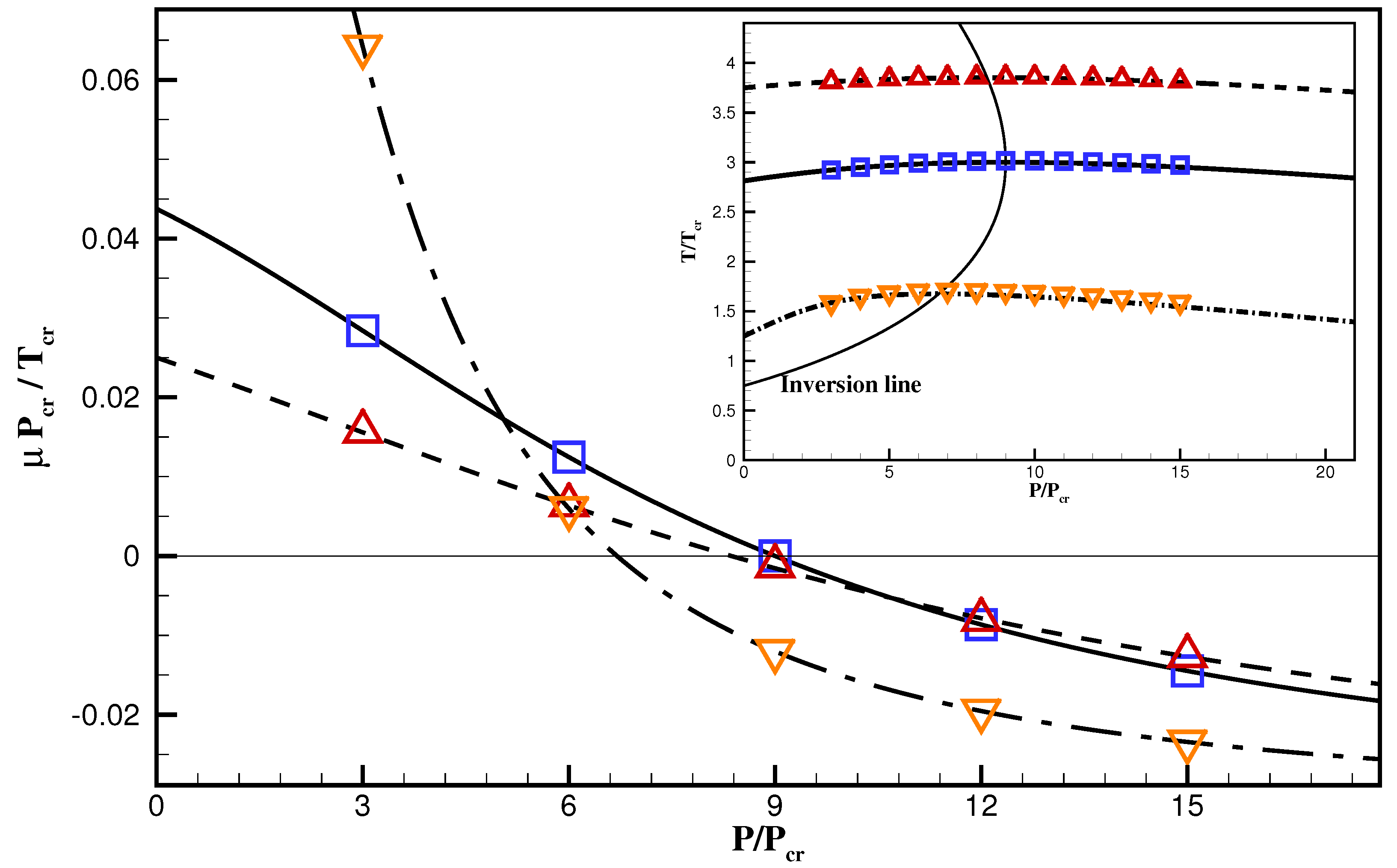
• As a first test of basic thermodynamic consistency for non-ideal fluids, we simulate the inversion line of a vdW fluid, which is one of the classic thermodynamical concepts of non-ideal fluids. To capture this phenomenon it is crucial that the model recovers the correct energy equation and can operate in a wide range of pressures and temperatures in the super-critical part of the phase diagram;
• Phase-change is the next fundamental process that is tested with our model. It is important to remind that since the full energy equation is recovered by our kinetic equations, phase-change emerges naturally in the proposed scheme and no additional ad-hoc phase-change model is required. In addition, we probe fast dynamics with temperatures near the critical point, where phase-change happens on short time scales;
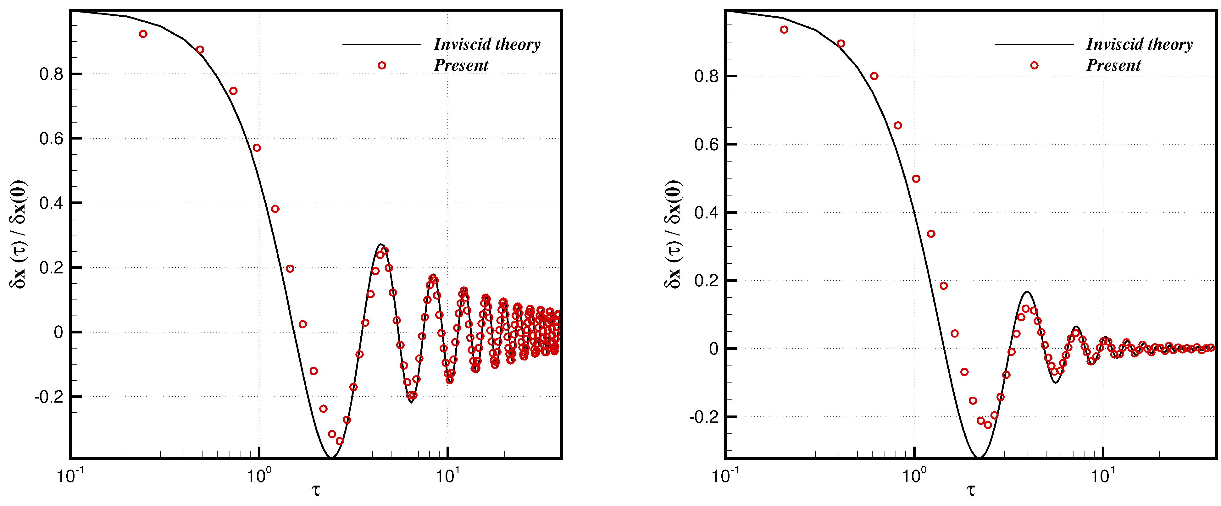
• As a final test case we probe both thermodynamic consistency as well as Galilean invariance in supersonic flows. In particular, we study the behavior of a perturbed shock-front in both an ideal gas as well as a vdW fluid at Mach number Ma = 3. In agreement with theory, our model shows to capture all regimes, including the exotic behaviors of a real fluid.

For all simulations, we use the standard D2Q9 lattice, where $D=2$ denotes the spatial dimension and $Q=9$ is the number of discrete velocities.

4.1. Inversion Line

When a fluid passes through a throttling device, the value of the enthalpy remains constant in the absence of work and heat. During this so-called throttling process, the pressure of the fluid drops and the behavior of the temperature is characterized by the Joule–Thomson (JT) coefficient $\mu ={\left(\partial T/\partial P\right)}_h$ [52]. Depending on the sign and value of the JT coefficient, the temperature may increase, decrease, or remain constant through the process. For ideal gas, the JT coefficient vanishes and thus the temperature does not change. On the other hand, for real gases, we need to distinguish between three different regions in the $T-P$ diagram, corresponding to the different signs of the Joule–Thomson coefficient. Let us start by defining the inversion line as the locus of points where $\mu =0$. Hence, crossing the inversion line will lead to a change of sign of $\mu$. For the vdW EOS, one can derive the expression for the inversion line as:

$$P_r=24\sqrt{3T_r}-12T_r-27,$$

(101)

where the subscript “r” indicates that the quantities are reduced with respect to their values at the critical point. The critical values of pressure, temperature and density for a vdW fluid are $P_{cr}=a/27b^2,T_{cr}=8a/27Rb$, and ${\rho }_{cr}=1/3b$, respectively. In addition to the reduced variables, it is useful to define the non-dimensional enthalpy as:

$$\widehat{h}=\frac{h}{R{T}_{cr}}=T_r\left[\frac{1}{\delta }+\frac{3}{3-{\rho }_r}\right]-\frac{9}{4}{\rho }_r,$$

(102)

where $\delta =R/C_v$ is a constant. A closer assessment of (101) reveals that the point with the maximum pressure on the inversion line corresponds to the following values, $\left(P_r,{\rho }_r,T_r,\widehat{h}\right)=\left(9.0,1.0,3.0,11.25\right)$.

To test that our model captures these phenomena also numerically, we measure the value of the Joule–Thomson coefficient at different points in the $T-P$ diagram. We do this in two steps, in the first simulation, the flow is subjected to a positive acceleration under fixed density hence the pressure drops and the quantity ${\left(\partial P/\partial T\right)}_{\rho }$ is measured. In a second simulation, the isothermal speed of sound ${\left(\partial P/\partial \rho \right)}_T$ is computed by introducing a small perturbation in the pressure field, measuring the velocity of the subsequent shock front. The Joule–Thomson coefficient is computed by:

$$\mu =-\frac{1}{C_p}\left[\frac{1}{\rho }-T\frac{{\left(\partial P/\partial T\right)}_{\rho }}{{\rho }^2{\left(\partial P/\partial \rho \right)}_T}\right].$$

(103)

Finally, we use a simple Euler scheme to construct the isenthalpic lines with:

$$\Delta T\approx \mu \Delta P.$$

(104)

The simulations are conducted for three different enthalpies, $\widehat{h}=5,\widehat{h}=11.25$, and $\widehat{h}=15$. Figure 2 shows the measured values of the dimensionless Joule–Thomson coefficient at different reduced pressures up to the far supercritical value $P_r=15$. The comparison between the van der Waals theory and the simulation is excellent and thus validates our scheme.

4.2. Phase Change: One-Dimensional Stefan Problem

In this section, we validate our model for phase-change problems, starting from the one-dimensional Stefan problem, where a liquid-vapor system is subjected to a heated wall on the vapor side. The heat transfer from the wall leads to the evaporation of liquid and the interface is moving away from the wall. The analytical solution for the liquid-vapor interface location with time is given by $x_i\left(t\right)=2\beta \sqrt{{\alpha }_{v}t}$, where ${\alpha }_v$ is the diffusivity of the vapor and $\beta$ is the solution to [53]:

$$\beta exp\left({\beta }^2\right)\mathrm{erf}\left(\beta \right)=\frac{\mathrm{St}}{\sqrt{\pi }},$$

(105)

where $\mathrm{St}=C_{pv}\Delta T/h_{fg}$ is the Stefan number, $C_{pv}$ is the specific heat capacity of the vapor phase, $\Delta T$ is the temperature difference between the wall, and the saturation temperature and $h_{fg}$ denotes the latent heat of evaporation. Simulations were carried out for three different Stefan numbers at fixed diffusivity. The choice of the Stefan number is directly related to the velocity of the interface:

$$\begin{array}{c}\hfill u_i\left(t\right)=\frac{d}{dt}{x}_i\left(t\right)=\beta \sqrt{\frac{{\alpha }_v}{t}},\end{array}$$

(106)

and hence the Mach number of the flow. Note that since our model is not restricted to low-speed flows, we can accurately capture a wide range of Stefan numbers. Figure 3 shows the location of the interface during evaporation compared to the analytical solution. The results of the simulation are in good agreement with the theory. We mention that the choice of parameters in our model such as the latent heat of evaporation $h_{fg}$ or the specific heat $C_p$ is not arbitrary and they are computed based on the thermodynamical state of the initial flow. For instance, the value of the Stefan number increases for a given temperature difference $\Delta T$ as we approach the critical point due to vanishing of $h_{fg}$ and diverging of $C_p$ at the critical point.

4.3. Phase Change: Nucleate Boiling

Due to its importance in engineering and real life applications, various boiling regimes have been the focus of many studies, both numerically and theoretically [48,54,55]. To validate our model, we chose a two-dimensional setup, where a liquid is in direct contact with a wall with high temperature in the middle of the wall. The schematic of the setup is shown in Figure 4a. The non-uniform temperature of the wall triggers a two-dimensional flow and the nucleus starts to appear and rise under the gravitational field. The nucleus continues to rise and grow until necking is achieved and the bubble is detaching from the nucleus. Once the first bubble is detached from the nucleus and released into the liquid, the nucleus continues to grow and releases a second bubble. This is a periodic process of bubble release, which is a function of surface tension, density ratio, and the gravity. An empirical correlation for the bubble release frequency was found experimentally by Zuber [56] and reads:

$$\begin{array}{c}\hfill f^{-1}\approx \frac{d}{0.59}{\left(\frac{\sigma g({\rho }_l-{\rho }_v)}{{\rho }_l^2}\right)}^{-1/4},\end{array}$$

(107)

where d is the departure diameter and is itself proportional to $g^{-0.5}$ [57], ${\rho }_l$ is the density of the liquid phase, and ${\rho }_v$ is that of the vapor phase. Hence, the bubble release period is proportional to $g^{-0.75}$. We consider a domain of $121\times 601$ points with time step $\delta t=0.3$, conductivity $k=0.6$, specific heat $C_v=3$, viscosity $\nu =0.005$, surface tension coefficient $\kappa =0.0234$, and gravity $g=0.0001$ in lattice units. The Jacob number is defined as:

$$\begin{array}{c}\hfill Ja=\frac{C_{pl}(T_w-T_{sat})}{h_{fg}},\end{array}$$

(108)

where $C_{pl}$ is the specific heat of the liquid phase. The wall temperature is set to $T_w=1.5T_{sat}$, where $T_{sat}$ is the saturation temperature and the initial temperature of the liquid is $T_{sat}=0.9T_{cr}$, which fixes the latent heat of evaporation. This choice of parameters leads to the Jacob number $Ja=2.21$. Figure 4b illustrates a sequence of the bubble interface from the early times of the first nucleus development until the first bubble is released into the liquid. The bubble release period was measured for different values of gravity and the results are presented in in Figure 5. The comparison shows that the bubble release period is proportional to $g^{-0.75}$ in our numerical simulations which is in agreement with the empirical correlation.

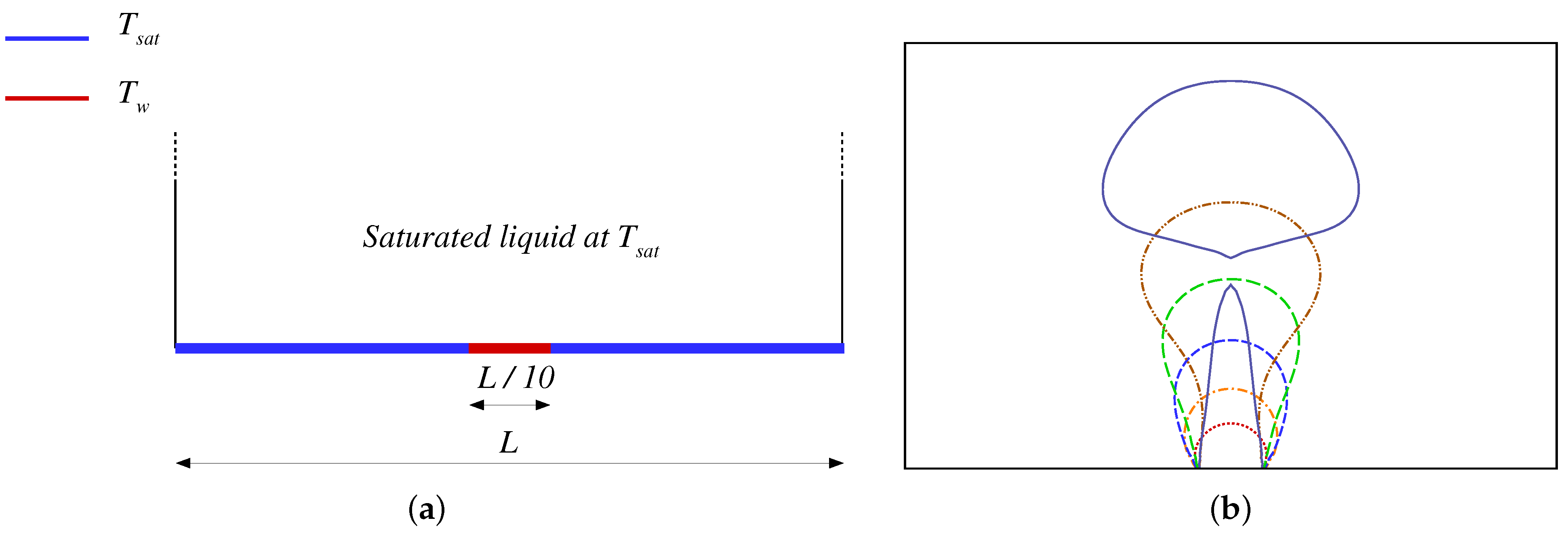
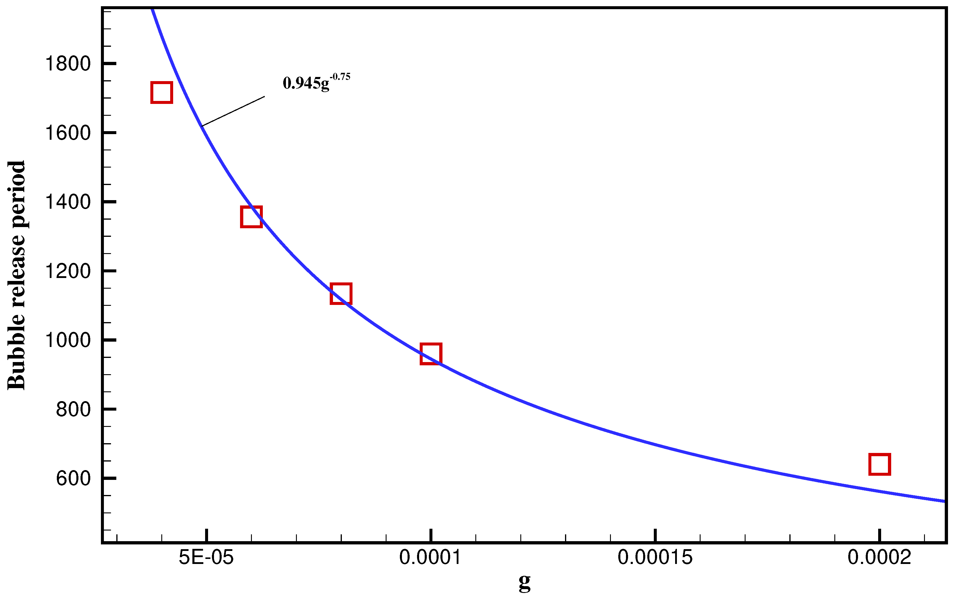
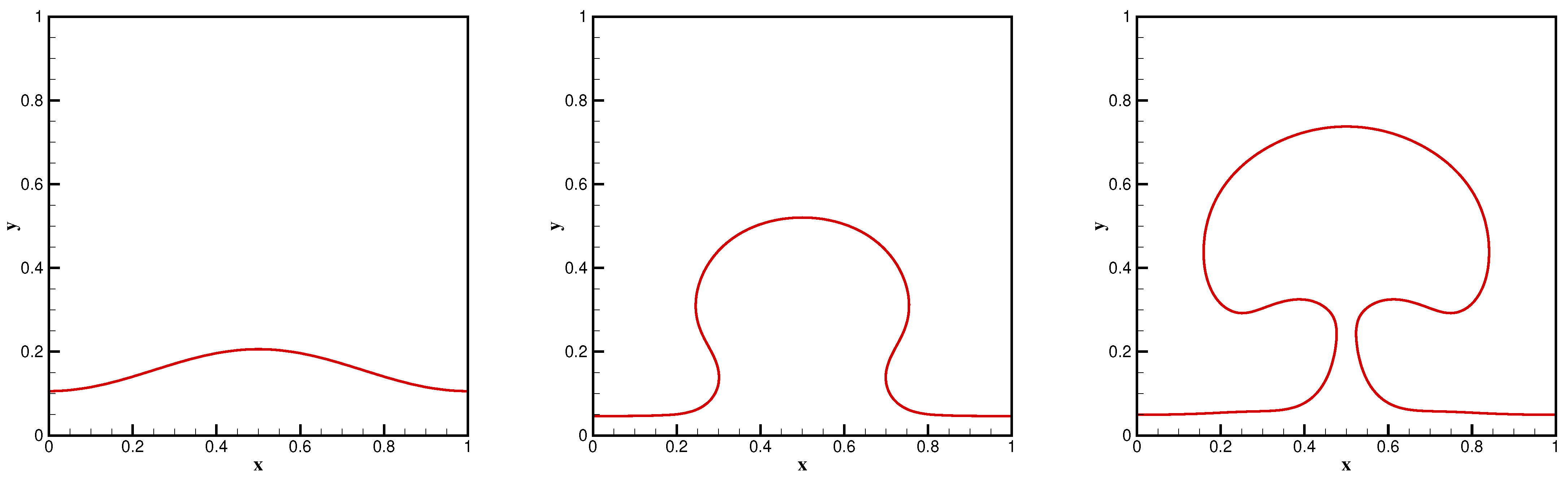
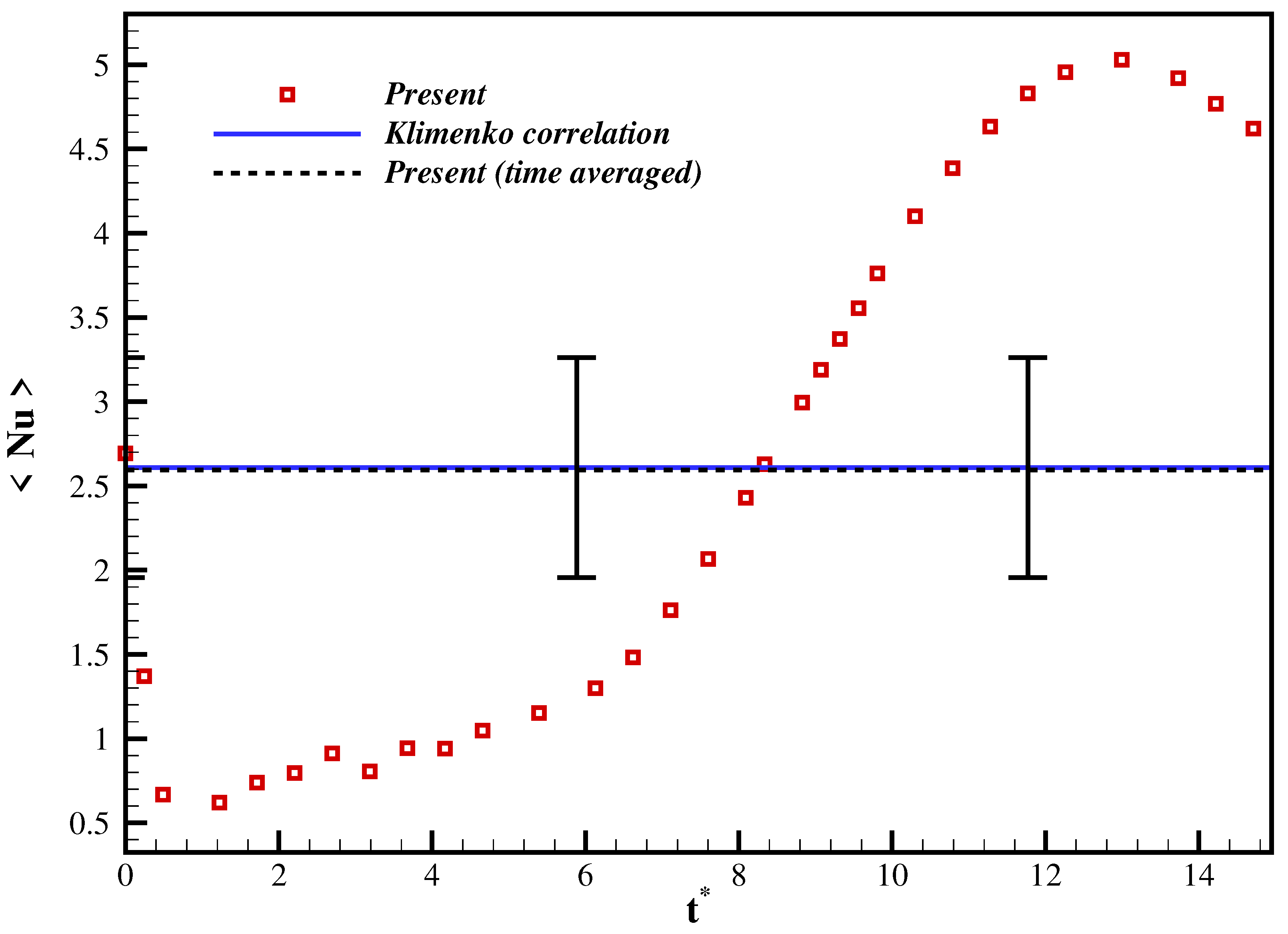
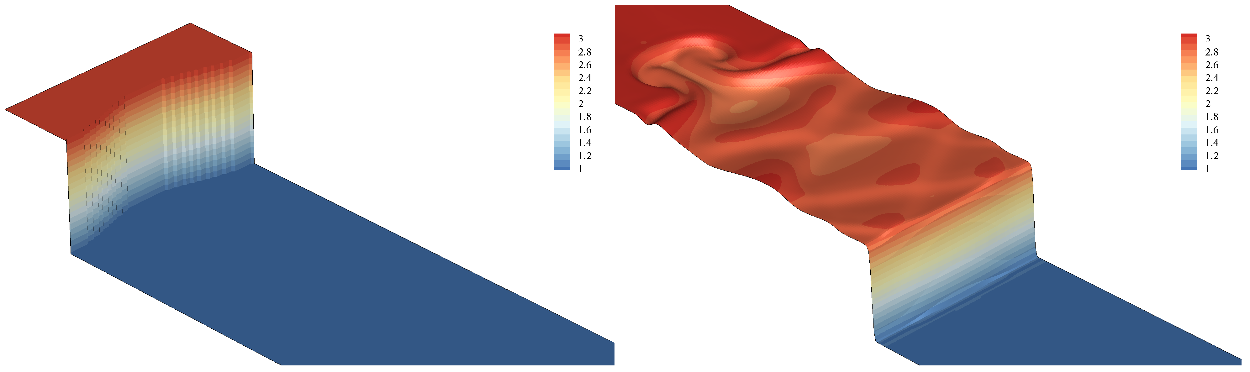
4.4. Phase Change: Single-Mode Film Boiling

As a final phase-change validation, we conduct simulations of film boiling, where a heated horizontal surface is covered by a thin layer of vapor. The liquid rests on top of the vapor and both phases are initially saturated. Phase-change then takes place at the liquid-vapor interface, where the heat is transported from the hot wall with temperature $T_w$, which is set to be above its saturation temperature $T_{sat}.$ The governing non-dimensional numbers are the Jacob, the Prandtl, and the Grashof number [58],

$$\begin{array}{cc}\hfill Ja& =\frac{C_{pv}(T_w-T_{sat})}{h_{fg}},\hfill \end{array}$$

(109)

$$\begin{array}{cc}\hfill Pr& =\frac{{\mu }_v{C}_{pv}}{k_v},\hfill \end{array}$$

(110)

$$\begin{array}{cc}\hfill Gr& ={\rho }_{v}g({\rho }_l-{\rho }_v)\frac{l_s^3}{{\mu }_v^2},\hfill \end{array}$$

(111)

which are defined for the vapor phase. The non-dimensional capillary length $l_s$ is defined as:

$$\begin{array}{c}\hfill l_s=\sqrt{\frac{\sigma }{({\rho }_l-{\rho }_v)g}},\end{array}$$

(112)

and $t^{*}=t/\sqrt{l_s/g}$ is the dimensionless time. The well-known Klimenko correlation as proposed in [59] has the following form in the laminar flow regime ($Gr\le 4.03\times {10}^5$):

$$\begin{array}{ccc}\hfill & N{u}_k=0.1691{\left(\frac{GrPr}{Ja}\right)}^{1/3},\hfill & \hfill Ja<0.71,\end{array}$$

(113)

$$\begin{array}{ccc}\hfill & N{u}_k=0.19{\left(GrPr\right)}^{1/3},\hfill & \hfill Ja\ge 0.71,\end{array}$$

(114)

where $Nu$ is the Nusselt number. In our simulation, we consider domain of $129\times 257$ points with $\delta t=0.3$, $k=0.6$, $C_v=3$, $\nu =0.005$, $\kappa =0.0234$ and $g=0.0001$ in lattice units. The non-dimensional numbers are $Ja=0.064,Pr=0.094$, and $Gr=2482.58$. Based on the value of the Jacob number, the Nusselt number as computed from the correlation (113) amounts to $N{u}_k=2.6085861$. Initially, the liquid-vapor interface is perturbed with the function:

$$\begin{array}{c}\hfill y=0.125W-0.05Wcos\left(\frac{2\pi x}{W}\right),\end{array}$$

(115)

where W is the width of the domain. The space-averaged Nusselt number is computed throughout the simulation using:

$$\begin{array}{c}\hfill \langle Nu\rangle =-\frac{l_s}{W(T_w-T_{sat})}{\int }_0^W\frac{\partial T}{\partial y}{|}_{w}dx,\end{array}$$

(116)

where the gradient of the temperature is computed at the wall using finite differences. The evolution of the liquid-vapor interface is shown at three different times in Figure 6. The first bubble is released at $t^{*}\approx 15$, which is then followed by a periodic release of bubbles. The space-averaged Nusselt number is computed during the simulations until the first bubble is released. The results are presented in Figure 7, where we have compared the time-averaged Nusselt number with the correlation (113). We can confirm the time-averaged Nusselt number is in very close agreement with the correlation while according to [59], the majority of the experimental data lie within $\pm 25\%$ interval of the fitted lines obtained by Equations (113) and (114).

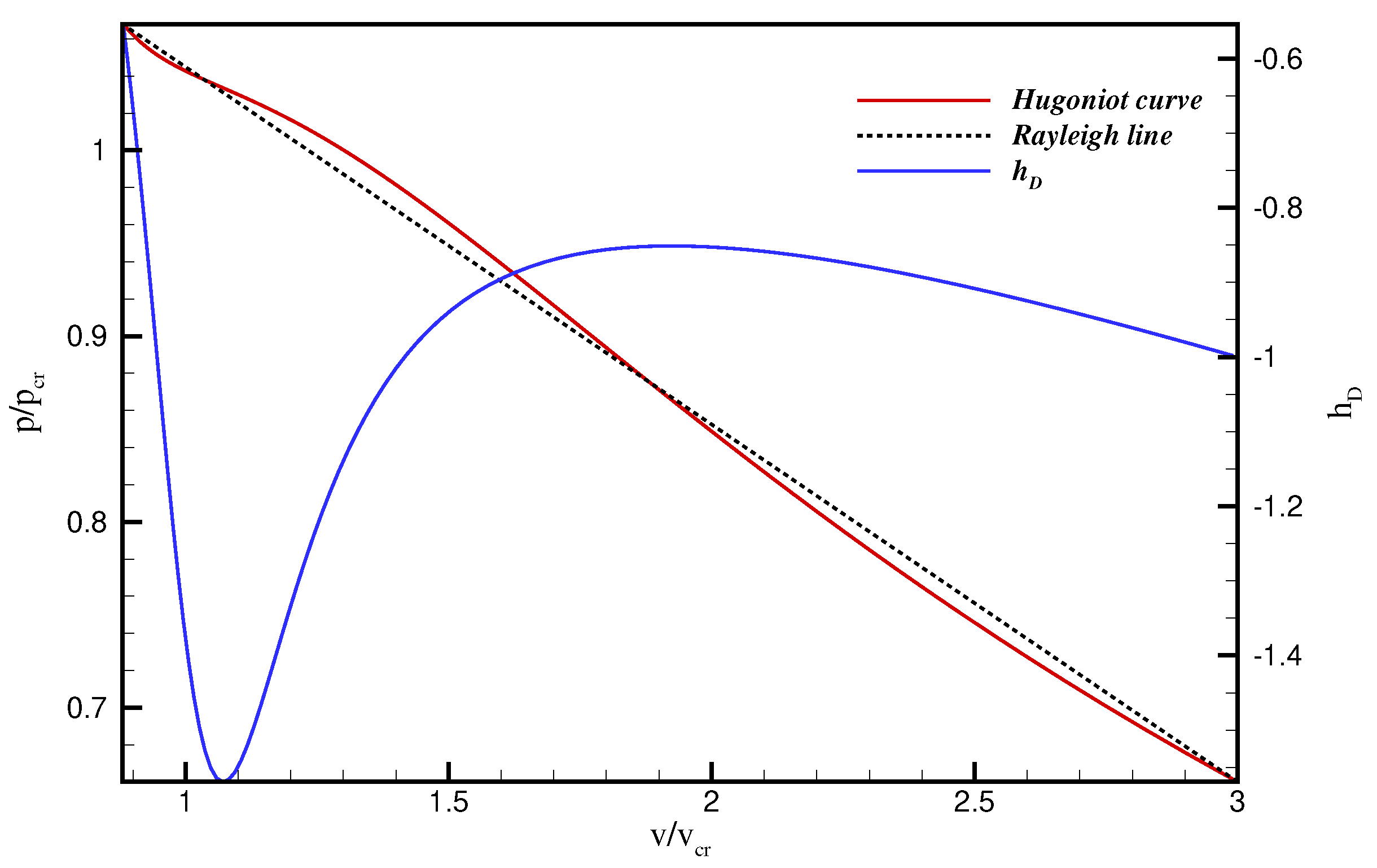
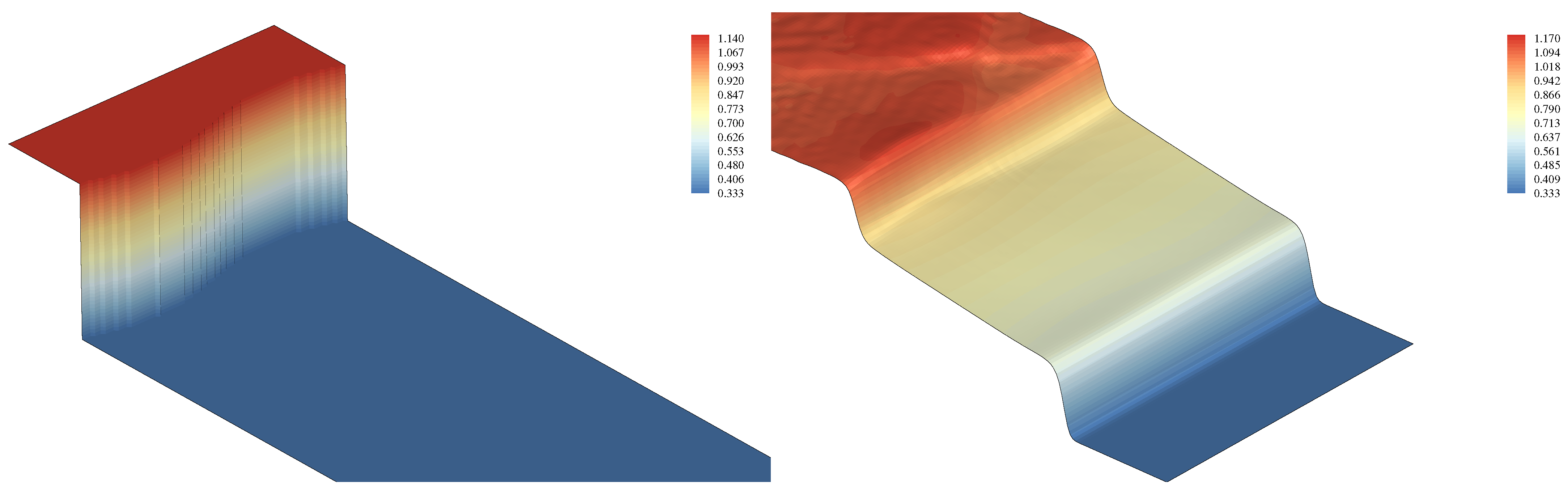
4.5. On the Stability of Shock Waves

The stability of planar shock waves subject to small perturbations have long been investigated since the pioneering work of D’yakov [60] and later modifications of Kontorovich [61], which were the first attempts to study the conditions under which a planar shock with corrugations on its surface would become unstable. The key parameter in the analysis of shock instabilities is the so called D’yakov parameter [20], defined as:

$$\begin{array}{c}\hfill h_D=j^2{\left(\frac{dv}{dp}\right)}_H,\end{array}$$

(117)

evaluated at the post-shock (downstream) state, where $j^2=(p_1-p_0)/(v_0-v_1)$ is the square of the mass flux across the shock front, v is the specific volume, p is the thermodynamic pressure, and the subscript H denotes that the derivative is taken along the Hugoniot curve [16].

Furthermore, the subscripts “0” and “1” refer to the upstream (pre-shock) and downstream (post-shock) states, respectively. It has been shown that the necessary condition for stability of a shock wave is [21,62]:

$$\begin{array}{c}\hfill -1<h_D<1+2M_1,\end{array}$$

(118)

where $0<M_1<1$ is the downstream Mach number, which is measured in the reference frame that is moving with the shock. Under this condition, linear perturbations imposed on the shock front will asymptotically decay in time as $t^{-3/2}$ [62].

According to the theory, a planar shock wave is unconditionally stable when propagating through an ideal-gas medium [63]. This can be easily evaluated, where h for an ideal gas EOS yields $h_{D,\mathrm{ig}}=-1/M_0^2$, which always falls within the stability range (118). On the other hand, for non-ideal fluids, these stability conditions (118) can be violated, which leads to an amplification of the perturbations until the structure of the flow filed is altered [62]. It has been shown that the violation of the upper limit of the stability condition (118) corresponds to the splitting of the shock front into two counter-propagating waves [64], while the violation of the lower limit is associated with the splitting of the shock front into two waves, travelling in the same direction [65].

Extensive theoretical investigations have been carried out to study the dynamics of the isolated planar shock waves propagating in an inviscid fluid medium. Namely, Bates [21,66] derived analytical expressions for the amplitude of the ripples on the shock front, for initial sinusoidal perturbations. According to [66], two families of solutions emerge depending on the sign of the following non-dimensional parameter:

$$\mathsf{\Lambda }={\alpha }^4-4\beta \mathsf{\Gamma }{\alpha }^2+4{\mathsf{\Gamma }}^2,$$

(119)

where

$$\begin{array}{c}\hfill {\alpha }^2=\frac{1-M_1^2}{M_1^2},\beta =\frac{1-h_{D_1}}{2M_1},\mathsf{\Gamma }=\frac{(1+h_D)\eta }{2M_1}\end{array}$$

(120)

are non-dimensional parameters as a function of downstream conditions and $\eta ={\rho }_1/{\rho }_0$ is the compression ratio through the shock. For the case $\mathsf{\Lambda }>0$, the solution is given by:

$$\begin{array}{cc}\hfill \frac{\delta x\left(\tau \right)}{\delta x\left(0\right)}=\frac{2{\alpha }^2\sqrt{{\beta }^2-1}}{\sqrt{\mathsf{\Lambda }}}{\int }_0^{\infty }& (bsinazcosbz-acosazsinbz)\frac{J_1(\alpha (\tau +z)}{\alpha (\tau +z)}dz,\hfill \end{array}$$

(121)

where $\delta x$ is the amplitude of the ripple, $\tau =Ukt/\eta$ is the non-dimensional time, U is the speed of the shock front in the laboratory reference of frame, k is the wave number of the initial ripple, $J_1$ is the first-kind Bessel function, and the parameters a and b are defined as:

$$\begin{array}{cc}\hfill a& =\sqrt{\frac{2\beta \mathsf{\Gamma }-{\alpha }^2}{4({\beta }^2-1)}+\frac{\mathsf{\Gamma }}{2{({\beta }^2-1)}^{1/2}}},\hfill \end{array}$$

(122)

$$\begin{array}{cc}\hfill b& =\sqrt{\frac{2\beta \mathsf{\Gamma }-{\alpha }^2}{4({\beta }^2-1)}-\frac{\mathsf{\Gamma }}{2{({\beta }^2-1)}^{1/2}}},\hfill \end{array}$$

(123)

and are real numbers. It is interesting to mention that the ideal-gas EOS belongs to this class of solutions. Using the asymptotic approximation $J_1\left(x\right)\sim \sqrt{2}{\left(\pi x\right)}^{-1/2}cos(x-3\pi /4)$ as $x\to \infty$ and considering Equation (121), one can confirm that the amplitude of the ripple in a fluid medium with $\mathsf{\Lambda }>0$ (such as an ideal gas) will decay in time with the negative power law ${\tau }^{-3/2}$ in the long-time limit [66].

However, the situation can be different for fluids with an EOS that can yield a negative $\mathsf{\Lambda }$. Finally, for the case $\mathsf{\Lambda }<0$, the solution to the initial value problem is [66]:

$$\begin{array}{cc}\hfill \frac{\delta x\left(\tau \right)}{\delta x\left(0\right)}& =\frac{1}{2}exp(-\sigma \tau )cosa\tau -\left[\frac{\mathsf{\Gamma }}{{\beta }^2-1}-\frac{{\alpha }^2}{2({\beta }^2-1)}\right]\frac{exp(-\sigma \tau )sina\tau }{4a\sigma }\hfill \\ \hfill & +\frac{{\alpha }^2}{4\sigma \sqrt{{\beta }^2-1}}\{{\int }_0^{\tau }exp\left(-\sigma (\tau -z)\right)\left(cosa(\tau -z)+\frac{\sigma }{a}sina(\tau -z)\right)\frac{J_1\left(\alpha z\right)}{\alpha z}dz\hfill \\ \hfill & +{\int }_0^{\infty }\left(cosaz+\frac{\sigma }{a}sinaz\right)\frac{J_1\left(\alpha (\tau +z)\right)}{\alpha (\tau +z)}dz\},\hfill \end{array}$$

(124)

where $\sigma =-ib$ is a real number. The presence of the exponential function implies a stronger damping compared to Equation (121). However, the long time asymptotic is still a function of ${\tau }^{-3/2}$ in both cases [66].

These theoretical considerations give us the opportunity to also test and validate our numerical model in the high-speed regime for the exotic shock-wave behavior of non-ideal gases. Our simulations consist of a long channel with periodic boundary conditions in the vertical direction. In all cases, the conductivity is set to zero and the viscosity is chosen to take the lowest possible value as long as the simulations are stable. In order to capture the shocks and avoid oscillations at the shock front, a third-order WENO scheme based on a 4-point stencil has been used in the reconstruction process instead of the third-order Lagrange polynomials in all previous simulations. Three different cases have been selected: Ideal gas (IG) with $M_0=3$, vdW fluid with $M_0=3.033$, and $M_0=1.114$. All other parameters are provided in

Table 1. Parameters for different cases of the simulation of the shock-stability.

Case	EOS	${\mathit{M}}_0$	${\mathit{\rho }}_0$	${\mathit{p}}_0$	$\mathit{\nu }$	$\mathit{\delta }\mathit{t}$	${\mathit{C}}_{\mathit{v}}/\mathit{R}$	${\mathit{h}}_{\mathit{D}}$	$\mathbf{\Lambda }$
(1)	IG	3.0	1	1	${10}^{-3}$	0.03	1.5	−1/9	4.214
(2)	vdW	3.033	${\rho }_{cr}/3$	$0.66p_{cr}$	${10}^{-4}$	0.1	3.0	−0.094	−7.856
(3)	vdW	1.114	${\rho }_{cr}/3$	$0.66p_{cr}$	${10}^{-6}$	0.4	80.0	−0.542	1.487

. In all cases, the shock front is initially perturbed with a single-mode sinusoidal function. The ratio of the amplitude to the wave length of the perturbation is $10\%$. The first two cases fall into the category of stable shocks, where the perturbations on the shock front are expected to decay in time. However, the last case is an example of shock-splitting, which will be discussed below.

Let us consider the first two cases. At time $t=0$, the shock starts to propagate while it oscillates as it moves further towards the low-pressure side. We then measure the oscillation amplitude and compare it to the analytical expressions.

The initial shape of the shock front and its evolution in time is shown in Figure 8 for the first case, where the oscillation of the front and the damping effect is apparent. Figure 9 shows the bird-eye view of this simulation.

According to the sign of $\mathsf{\Lambda }$, the magnitude of the ripple for case (1) and case (2) were compared with analytical solutions (121) and (124), respectively. The results are presented in Figure 10 and are in good agreement with the theory. It is apparent that our model captured the two distinct damping effects accurately, with a more pronounced damping for the non-ideal fluid, as expected.

We now consider the exotic case (3). As mentioned earlier, non-ideal fluids can show exotic behaviors under certain conditions. Regarding case (3), due to its large specific heat value, the Hugoniot curve passes through regions, where the relation $h_D<-1$ is satisfied. As argued in [16], this, together with the fact that the Hugoniot curve has more than two intersection points with the Rayleigh line (see Figure 11) can cause the shock front to split into two traveling waves. Figure 12 presents our simulation for this case, where it is visible that the initial perturbation on the shock front has become unstable, leading to splitting of the shock. The resulting waves travel in the same direction with different speeds, as expected. This validates our model also for high-speed flows and shock-waves in real-gas media.

5. Conclusions

In this paper, we presented a thorough study of our recently proposed model for compressible non-ideal flows. The model features full Galilean-invariance and the full energy equation is recovered for a non-ideal fluid, accounting also for two-phase systems and the presence of interfaces. It has been shown that the model is able to handle flows which are far into supercritical states. The effect of the inversion line on the $T-P$ diagram was correctly captured for the van der Waals fluid in a wide range of reduced-pressures, from $p_r=3$ to $p_r=15$. In addition, owing to the full energy conservation, the latent heat is already included in the model. This was shown on two different phase-change benchmarks: The one-dimensional Stefan problem and boiling. As one of the advantages of the model, we were able to choose relatively large Stefan and Jacob numbers, which are scarce in the literature. Finally, the stability of an initially perturbed shock front in ideal gas and in the van der Waals fluid at a Mach number $\mathrm{Ma}\approx 3$ were studied and compared to theoretical predictions. It was observed that the damping effect was much stronger in the nonideal fluid as predicted by the inviscid theory. Beside from the fact that all of these simulations were implemented by taking only nine discrete velocities in two dimensions, the results show that the real-gas effects were captured accurately by the proposed model.

References

1. Atif, M.; Kolluru, P.K.; Thantanapally, C.; Ansumali, S. Essentially Entropic Lattice Boltzmann Model. Phys. Rev. Lett. 2017, 119, 240602. [Google Scholar] [CrossRef] [PubMed]
2. Dorschner, B.; Bösch, F.; Chikatamarla, S.S.; Boulouchos, K.; Karlin, I.V. Entropic multi-relaxation time lattice Boltzmann model for complex flows. J. Fluid Mech. 2016, 801, 623–651. [Google Scholar] [CrossRef]
3. Kunert, C.; Harting, J. Roughness Induced Boundary Slip in Microchannel Flows. Phys. Rev. Lett. 2007, 99, 176001. [Google Scholar] [CrossRef] [PubMed]
4. Hyväluoma, J.; Harting, J. Slip Flow Over Structured Surfaces with Entrapped Microbubbles. Phys. Rev. Lett. 2008, 100, 246001. [Google Scholar] [CrossRef] [PubMed]
5. Sbragaglia, M.; Benzi, R.; Biferale, L.; Succi, S.; Toschi, F. Surface Roughness-Hydrophobicity Coupling in Microchannel and Nanochannel Flows. Phys. Rev. Lett. 2006, 97, 204503. [Google Scholar] [CrossRef] [PubMed]
6. Biferale, L.; Perlekar, P.; Sbragaglia, M.; Toschi, F. Convection in Multiphase Fluid Flows Using Lattice Boltzmann Methods. Phys. Rev. Lett. 2012, 108, 104502. [Google Scholar] [CrossRef]
7. Benzi, R.; Chibbaro, S.; Succi, S. Mesoscopic Lattice Boltzmann Modeling of Flowing Soft Systems. Phys. Rev. Lett. 2009, 102, 026002. [Google Scholar] [CrossRef]
8. Mazloomi, M.A.; Chikatamarla, S.S.; Karlin, I.V. Entropic Lattice Boltzmann Method for Multiphase Flows. Phys. Rev. Lett. 2015, 114, 174502. [Google Scholar] [CrossRef]
9. Succi, S. The Lattice Boltzmann Equation: For Complex States of Flowing Matter; Oxford University Press: Oxford, UK, 2018. [Google Scholar]
10. Krüger, T.; Kusumaatmaja, H.; Kuzmin, A.; Shardt, O.; Silva, G.; Viggen, E.M. The lattice Boltzmann method. Springer Int. Publ. 2017, 10, 4–15. [Google Scholar]
11. Prasianakis, N.I.; Karlin, I.V. Lattice Boltzmann method for simulation of compressible flows on standard lattices. Phys. Rev. E 2008, 78, 016704. [Google Scholar] [CrossRef]
12. Frapolli, N.; Chikatamarla, S.S.; Karlin, I.V. Entropic lattice Boltzmann model for compressible flows. Phys. Rev. E 2015, 92, 061301. [Google Scholar] [CrossRef] [PubMed]
13. Dorschner, B.; Bösch, F.; Karlin, I.V. Particles on Demand for Kinetic Theory. Phys. Rev. Lett. 2018, 121, 130602. [Google Scholar] [CrossRef] [PubMed]
14. Feng, Y.; Boivin, P.; Jacob, J.; Sagaut, P. Hybrid recursive regularized thermal lattice Boltzmann model for high subsonic compressible flows. J. Comput. Phys. 2019, 394, 82–99. [Google Scholar] [CrossRef]
15. Wilde, D.; Krämer, A.; Reith, D.; Foysi, H. Semi-Lagrangian lattice Boltzmann method for compressible flows. Phys. Rev. E 2020, 101, 053306. [Google Scholar] [CrossRef]
16. Bates, J.W.; Montgomery, D.C. Some numerical studies of exotic shock wave behavior. Phys. Fluids 1999, 11, 462–475. [Google Scholar] [CrossRef]
17. Zhao, N.; Mentrelli, A.; Ruggeri, T.; Sugiyama, M. Admissible shock waves and shock-induced phase transitions in a van der Waals fluid. Phys. Fluids 2011, 23, 086101. [Google Scholar] [CrossRef]
18. Guardone, A.; Vigevano, L. Roe linearization for the van der Waals gas. J. Comput. Phys. 2002, 175, 50–78. [Google Scholar] [CrossRef]
19. Zamfirescu, C.; Guardone, A.; Colonna, P. Admissibility region for rarefaction shock waves in dense gases. J. Fluid Mech. 2008, 599, 363–381. [Google Scholar] [CrossRef]
20. Bates, J.W.; Montgomery, D.C. The D’yakov-Kontorovich instability of shock waves in real gases. Phys. Rev. Lett. 2000, 84, 1180. [Google Scholar] [CrossRef]
21. Bates, J.W. Instability of isolated planar shock waves. Phys. Fluids 2007, 19, 094102. [Google Scholar] [CrossRef]
22. Swift, M.R.; Osborn, W.; Yeomans, J. Lattice Boltzmann simulation of nonideal fluids. Phys. Rev. Lett. 1995, 75, 830. [Google Scholar] [CrossRef] [PubMed]
23. Holdych, D.; Rovas, D.; Georgiadis, J.G.; Buckius, R. An improved hydrodynamics formulation for multiphase flow lattice-Boltzmann models. Int. J. Mod. Phys. C 1998, 9, 1393–1404. [Google Scholar] [CrossRef]
24. Guo, Z.; Zheng, C.; Shi, B. Discrete lattice effects on the forcing term in the lattice Boltzmann method. Phys. Rev. E 2002, 65, 046308. [Google Scholar] [CrossRef] [PubMed]
25. Huang, H.; Krafczyk, M.; Lu, X. Forcing term in single-phase and Shan-Chen-type multiphase lattice Boltzmann models. Phys. Rev. E 2011, 84, 046710. [Google Scholar] [CrossRef] [PubMed]
26. Lycett-Brown, D.; Luo, K.H. Improved forcing scheme in pseudopotential lattice Boltzmann methods for multiphase flow at arbitrarily high density ratios. Phys. Rev. E 2015, 91, 023305. [Google Scholar] [CrossRef] [PubMed]
27. Wagner, A.; Li, Q. Investigation of Galilean invariance of multi-phase lattice Boltzmann methods. Phys. A: Stat. Mech. Its Appl. 2006, 362, 105–110. [Google Scholar] [CrossRef]
28. Inamuro, T.; Konishi, N.; Ogino, F. A Galilean invariant model of the lattice Boltzmann method for multiphase fluid flows using free-energy approach. Comput. Phys. Commun. 2000, 129, 32–45. [Google Scholar] [CrossRef]
29. He, X.; Doolen, G.D. Thermodynamic foundations of kinetic theory and lattice Boltzmann models for multiphase flows. J. Stat. Phys. 2002, 107, 309–328. [Google Scholar] [CrossRef]
30. Swift, M.R.; Orlandini, E.; Osborn, W.; Yeomans, J. Lattice Boltzmann simulations of liquid-gas and binary fluid systems. Phys. Rev. E 1996, 54, 5041. [Google Scholar] [CrossRef]
31. Moqaddam, A.M.; Chikatamarla, S.S.; Karlin, I.V. Simulation of droplets collisions using two-phase entropic lattice boltzmann method. J. Stat. Phys. 2015, 161, 1420–1433. [Google Scholar] [CrossRef]
32. Bösch, F.; Dorschner, B.; Karlin, I. Entropic multi-relaxation free-energy lattice Boltzmann model for two-phase flows. EPL Europhys. Lett. 2018, 122, 14002. [Google Scholar] [CrossRef]
33. Moqaddam, A.M.; Chikatamarla, S.S.; Karlin, I.V. Drops bouncing off macro-textured superhydrophobic surfaces. J. Fluid Mech. 2017, 824, 866–885. [Google Scholar] [CrossRef]
34. Dorschner, B.; Chikatamarla, S.S.; Karlin, I.V. Fluid-structure interaction with the entropic lattice Boltzmann method. Phys. Rev. E 2018, 97, 023305. [Google Scholar] [CrossRef] [PubMed]
35. Zhang, R.; Chen, H. Lattice Boltzmann method for simulations of liquid-vapor thermal flows. Phys. Rev. E 2003, 67, 066711. [Google Scholar] [CrossRef]
36. Fei, L.; Yang, J.; Chen, Y.; Mo, H.; Luo, K.H. Mesoscopic simulation of three-dimensional pool boiling based on a phase-change cascaded lattice Boltzmann method. Phys. Fluids 2020, 32, 103312. [Google Scholar] [CrossRef]
37. Kamali, M.; Gillissen, J.; Van den Akker, H.; Sundaresan, S. Lattice-Boltzmann-based two-phase thermal model for simulating phase change. Phys. Rev. E 2013, 88, 033302. [Google Scholar] [CrossRef]
38. Safari, H.; Rahimian, M.H.; Krafczyk, M. Extended lattice Boltzmann method for numerical simulation of thermal phase change in two-phase fluid flow. Phys. Rev. E 2013, 88, 013304. [Google Scholar] [CrossRef]
39. Kupershtokh, A.L.; Medvedev, D.A.; Gribanov, I.I. Thermal lattice Boltzmann method for multiphase flows. Phys. Rev. E 2018, 98, 023308. [Google Scholar] [CrossRef]
40. Reyhanian, E.; Rahimian, M.H.; Chini, S.F. Investigation of 2D drop evaporation on a smooth and homogeneous surface using Lattice Boltzmann method. Int. Commun. Heat Mass Transf. 2017, 89, 64–72. [Google Scholar] [CrossRef]
41. Reyhanian, E.; Dorschner, B.; Karlin, I.V. Thermokinetic lattice Boltzmann model of nonideal fluids. Phys. Rev. E 2020, 102, 020103. [Google Scholar] [CrossRef]
42. Krämer, A.; Küllmer, K.; Reith, D.; Joppich, W.; Foysi, H. Semi-Lagrangian off-lattice Boltzmann method for weakly compressible flows. Phys. Rev. E 2017, 95, 023305. [Google Scholar] [CrossRef] [PubMed]
43. Di Ilio, G.; Dorschner, B.; Bella, G.; Succi, S.; Karlin, I.V. Simulation of turbulent flows with the entropic multirelaxation time lattice Boltzmann method on body-fitted meshes. J. Fluid Mech. 2018, 849, 35–56. [Google Scholar] [CrossRef]
44. Shan, X.; He, X. Discretization of the velocity space in the solution of the Boltzmann equation. Phys. Rev. Lett. 1998, 80, 65. [Google Scholar] [CrossRef]
45. Ansumali, S.; Karlin, I.V. Kinetic boundary conditions in the lattice Boltzmann method. Phys. Rev. E 2002, 66, 026311. [Google Scholar] [CrossRef] [PubMed]
46. Grad, H. On the kinetic theory of rarefied gases. Commun. Pure Appl. Math. 1949, 2, 331–407. [Google Scholar] [CrossRef]
47. Kupershtokh, A.; Medvedev, D.; Karpov, D. On equations of state in a lattice Boltzmann method. Comput. Math. Appl. 2009, 58, 965–974. [Google Scholar] [CrossRef]
48. Liu, J. Thermal Convection in the van der Waals Fluid. In Frontiers in Computational Fluid-Structure Interaction and Flow Simulation; Springer International Publishing: Cham, Switzerland, 2018; pp. 377–398. [Google Scholar]
49. Li, Q.; Zhou, P.; Yan, H. Revised Chapman-Enskog analysis for a class of forcing schemes in the lattice Boltzmann method. Phys. Rev. E 2016, 94, 043313. [Google Scholar] [CrossRef]
50. Lycett-Brown, D.; Luo, K.H. Multiphase cascaded lattice Boltzmann method. Comput. Math. Appl. 2014, 67, 350–362. [Google Scholar] [CrossRef]
51. Wagner, A. Thermodynamic consistency of liquid-gas lattice Boltzmann simulations. Phys. Rev. E 2006, 74, 056703. [Google Scholar] [CrossRef]
52. Cengel, Y.A.; Boles, M.A. Thermodynamics: An Engineering Approach 6th Editon (SI Units); The McGraw-Hill Companies, Inc.: New York, NY, USA, 2007. [Google Scholar]
53. Welch, S.W.; Wilson, J. A volume of fluid based method for fluid flows with phase change. J. Comput. Phys. 2000, 160, 662–682. [Google Scholar] [CrossRef]
54. Onuki, A. Dynamic van der Waals theory of two-phase fluids in heat flow. Phys. Rev. Lett. 2005, 94, 054501. [Google Scholar] [CrossRef] [PubMed]
55. Onuki, A. Dynamic van der Waals theory. Phys. Rev. E 2007, 75, 036304. [Google Scholar] [CrossRef] [PubMed]
56. Zuber, N. Nucleate boiling. The region of isolated bubbles and the similarity with natural convection. Int. J. Heat Mass Transf. 1963, 6, 53–78. [Google Scholar] [CrossRef]
57. Kocamustafaogullari, G. Pressure dependence of bubble departure diameter for water. Int. Commun. Heat Mass Transf. 1983, 10, 501–509. [Google Scholar] [CrossRef]
58. Esmaeeli, A.; Tryggvason, G. Computations of film boiling. Part I: Numerical method. Int. J. Heat Mass Transf. 2004, 47, 5451–5461. [Google Scholar] [CrossRef]
59. Klimenko, V.; Shelepen, A. Film boiling on a horizontal plate—A supplementary communication. Int. J. Heat Mass Transf. 1982, 25, 1611–1613. [Google Scholar] [CrossRef]
60. D’yakov, S. Shock wave stability. Zh. Eksp. Teor. Fiz 1954, 27, 288–295. [Google Scholar]
61. Kontorovich, V.M. Concerning the stability of shock waves. Sov. Phys. JETP 1957, 6, 1179–1180. [Google Scholar]
62. Bates, J. On the theory of a shock wave driven by a corrugated piston in a non-ideal fluid. J. Fluid Mech. 2012, 691, 146–164. [Google Scholar] [CrossRef]
63. Landau, L.D.; Lifshitz, E.M. Fluid Mechanics, 2nd ed.; Pergamon Press: Oxford, UK, 1987; pp. 61–252. [Google Scholar]
64. Gardner, C. Comment on“Stability of Step Shocks”. Phys. Fluids 1963, 6, 1363–1367. [Google Scholar] [CrossRef]
65. Bethe, H. The Theory of Shock Waves for an Arbitrary Equation of State; Report No PB-32189; Clearinghouse for Federal Scientific and Technical Information, US Department of Commerce: Washington, DC, USA, 1942. [Google Scholar]
66. Bates, J.W. Initial-value-problem solution for isolated rippled shock fronts in arbitrary fluid media. Phys. Rev. E 2004, 69, 056313. [Google Scholar] [CrossRef] [PubMed]
Figure 1. Flowchart of the semi-Lagrangian advection using the predictor-corrector algorithm.
Computation 09 00013 g001
Figure 2. Joule-Thomson coefficient against reduced pressure. The value of the Joule–Thomson coefficient along the dimensionless isenthalpic lines h ^ = h / R T c r was measured in a wide range of reduced pressures up to P / P c r = 15 . Line: Theory; Solid: h ^ = 11.25 ; Dashed: h ^ = 15 ; Dash dot: h ^ = 5 . Symbols: Present method; Squares: h ^ = 11.25 ; Triangles: h ^ = 15 ; Inverted triangles: h ^ = 5 . Inset: Simulated lines of constant enthalpy on the T r P r (phase) diagram.
Computation 09 00013 g002
Figure 3. Location of the interface versus time in lattice units for four different Stefan numbers. Line: Analytical solution. Symbols: Present method.
Computation 09 00013 g003
Figure 4. (a) Schematic of the nucleate problem. (b) The interface of the vapor bubble during the nucleation, starting from the appearance of the first nucleus until the release of the first bubble. From bottom to top; Fine-dashed: Time = 600, Dash dot: Time = 1200, Dashed: Time = 1800, Long-dashed: Time = 2400, Dash dot-dot: Time = 3000, Solid: Time = 3780. Times are measured in lattice units.
Computation 09 00013 g004
Figure 5. Bubble release period against different gravity numbers. Symbols: Simulation. The solid line represents a function 0.945 g 0.75 .
Computation 09 00013 g005
Figure 6. Bubble growth from the vapor film at G r = 2482.58 , J a = 0.064 , and P r = 0.094 . The phase boundary is shown at different times. From left to right: t * = 0 , t * = 9.8 , and t * = 14.96 .
Computation 09 00013 g006
Figure 7. Space-averaged Nusselt number as a function of dimensionless time for G r = 2482.58 , J a = 0.064 , and P r = 0.094 . The error bars amount to ± 25 % acceptable error as shown by Klimenko [59].
Computation 09 00013 g007
Figure 8. Evolution of an initially perturbed shock (dashed line) in time in an ideal gas medium with γ = 5 / 3 and Ma = 3.0 .
Computation 09 00013 g008
Figure 9. Case(1): Left: Initial perturbation on the shock front. Right: Evolution of the shock-front at time τ = 9.73 . Both plots and their coloring, show reduced density with respect to the pre-shock value ρ / ρ 0 .
Computation 09 00013 g009
Figure 10. Comparison between the theoretical solution and the simulations for the ripple amplitude of an initially perturbed shock propagating through (left) an ideal gas with M 0 = 3.0 (right) a van der Waals (vdW) fluid with M 0 = 3.033 .
Computation 09 00013 g010
Figure 11. Case(3): The plot of h D and the Hugoniot curve as a function of the downstream specific volume. It is visible that the Hugoniot curve has more than two intersection points with the Rayleigh line. In addition, as the volume decreases, there are regions where h D < 1 .
Computation 09 00013 g011
Figure 12. Case(3): Left: Initial perturbation on the shock front. Right: Evolution of the shock-front at time τ = 16.3 . The shock wave has split into two travelings waves in the same direction. Both plots and their coloring show reduced density with respect to the critical value ρ / ρ c r .
Computation 09 00013 g012