
Weighted Consensus Segmentations
by
 , , , and
Halima Saker
1,2 ,
,
Rainer Machné
3,
Jörg Fallmann
1,
Douglas B. Murray
4,5,
Ahmad M. Shahin
2 and
Peter F. Stadler
1,6,7,8,9,* 1
Bioinformatics Group, Department of Computer Science, and Interdisciplinary Center for Bioinformatics, Universität Leipzig, D-04107 Leipzig, Germany
2
Doctoral School of Science and Technology, Lebanese University, Tripoli, Lebanon
3
Institute for Synthetic Microbiology and Institute for Quantitative and Theoretical Biology, Heinrich Heine University, D-40225 Düsseldorf, Germany
4
Lakeland University Japan Shinjuku-ku, Tokyo 160-0022, Japan
5
University of Maryland Global Campus—Asia, Yokota Air Base, Fussa-shi, Tokyo 197-0001, Japan
6
German Centre for Integrative Biodiversity Research (iDiv) Halle-Jena-Leipzig, Competence Center for Scalable Data Services and Solutions, Leipzig Research Center for Civilization Diseases, and Leipzig Research Center for Civilization Diseases (LIFE), Leipzig University, D-04103 Leipzig, Germany
7
Institute for Theoretical Chemistry, University of Vienna, A-1090 Wien, Austria
8
Facultad de Ciencias, Universidad National de Colombia, Bogotá CO-111321, Colombia
9
Santa Fe Institute, Santa Fe, NM 87501, USA
*
Author to whom correspondence should be addressed.
Computation 2021, 9(2), 17; https://0-doi-org.brum.beds.ac.uk/10.3390/computation9020017
Submission received: 31 December 2020
/
Revised: 22 January 2021
/
Accepted: 27 January 2021
/
Published: 5 February 2021
(This article belongs to the Special Issue Bioinformatics Tools for ncRNAs)
Abstract
:The problem of segmenting linearly ordered data is frequently encountered in time-series analysis, computational biology, and natural language processing. Segmentations obtained independently from replicate data sets or from the same data with different methods or parameter settings pose the problem of computing an aggregate or consensus segmentation. This Segmentation Aggregation problem amounts to finding a segmentation that minimizes the sum of distances to the input segmentations. It is again a segmentation problem and can be solved by dynamic programming. The aim of this contribution is (1) to gain a better mathematical understanding of the Segmentation Aggregation problem and its solutions and (2) to demonstrate that consensus segmentations have useful applications. Extending previously known results we show that for a large class of distance functions only breakpoints present in at least one input segmentation appear in the consensus segmentation. Furthermore, we derive a bound on the size of consensus segments. As show-case applications, we investigate a yeast transcriptome and show that consensus segments provide a robust means of identifying transcriptomic units. This approach is particularly suited for dense transcriptomes with polycistronic transcripts, operons, or a lack of separation between transcripts. As a second application, we demonstrate that consensus segmentations can be used to robustly identify growth regimes from sets of replicate growth curves.
1. Introduction
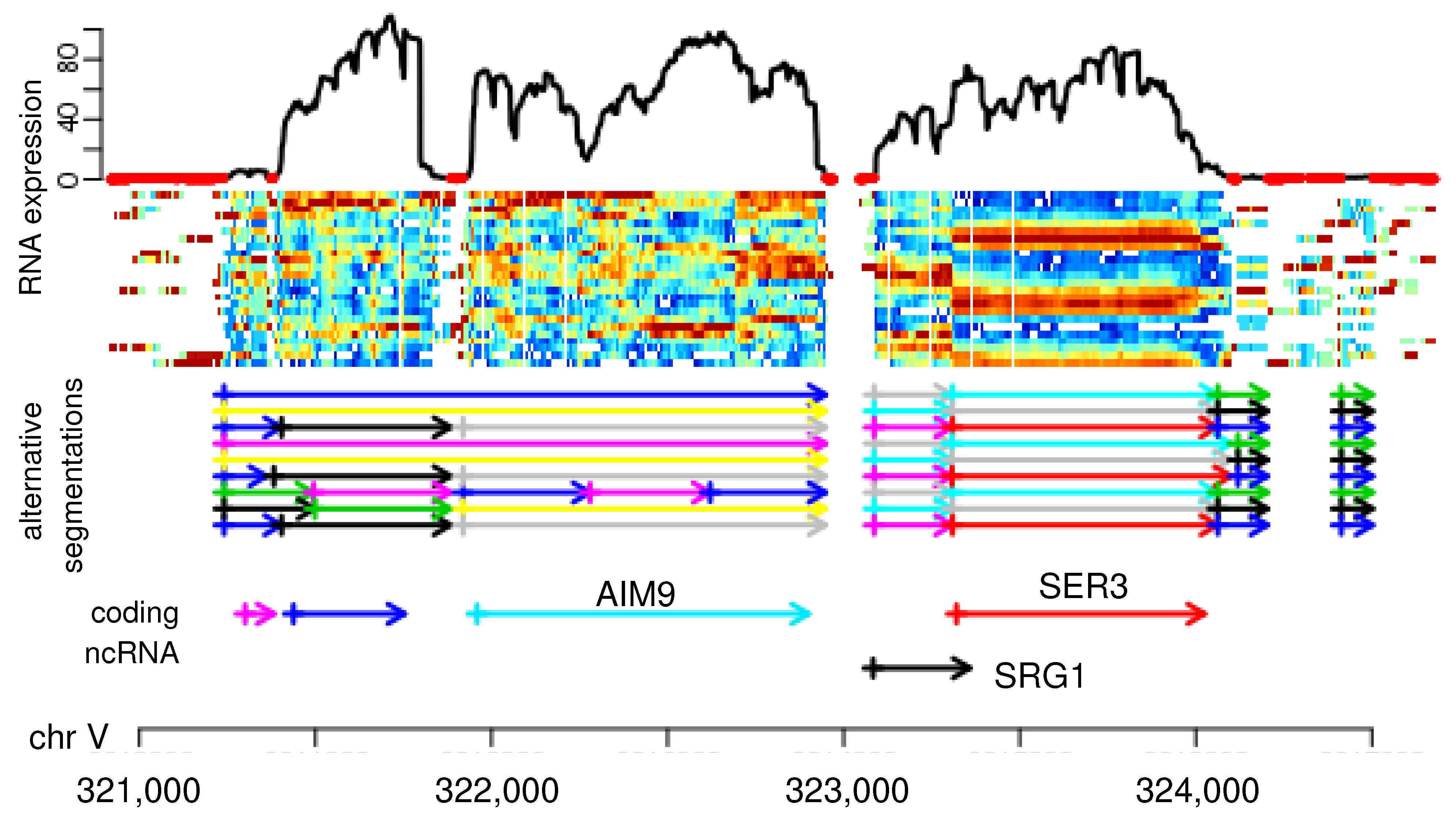
One-dimensional segmentation problems naturally appear in time series analysis across diverse application areas (often referred to as change point or jump point detection in this context). In computational biology, 1D-segmentation problems arise in the analysis of micro-array and high-throughput DNA or RNA sequencing data. Copy number variations in genomes, for example, can be detected by segmenting array-CGH or DNA coverage data into piece-wise constant segments; see Reference [1] for a review. In epigenomics, recurrent patterns of histone modifications define genomic intervals that can be associated with functional units including promoters, enhancers, or gene bodies, see, e.g., Reference [2] and the references therein. The identification of transcriptional units is also a segmentation problem, consisting in the distinction of expressed and non-expressed loci [3,4] or operons [5] or, more generally, in the distinction of adjacent or even overlapping transcripts without the benefit of non-expressed spacers between them. The latter task is particularly relevant in organisms with “compact” genomes, such as bacteria [5] or yeast [6,7], where transcribed loci are rarely separated non-expressed regions. Boundaries between transcriptional units are detectable by differences in RNA levels [6], see, e.g., the SRG1 ncRNA in Figure 1. A plethora of segmentation algorithms for genomic features, as well as time series data, have become available, reviewed and benchmarked, e.g., in References [8,9,10].
The boundaries between segments typically are not clearly visible in individual data tracks. Such limitations can often be alleviated by aggregating multiple experiments or measurements. In the yeast RNA-seq data shown in Figure 1, for instance, transcriptome samples at different time points of the respiratory cycle are aggregated to produce a more informative signal than just the RNA expression level at a single time point. Still, any particular choice of parameters (here the choice of the similarity measure for the temporal coverage profiles at adjacent nucleotides), produce both false positive and false negative segment boundaries.
Figure 1 suggests that an improvement could be achieved by aggregating the different segmentations to a single consensus. In a similar vein, Reference [4] employed a simple heuristic segmentation to detect candidate loci as intervals that are scored by a statistical model for each RNA-seq experiment, followed by a problem-specific greedy heuristic to determine consensus interval boundaries for expressed ncRNA loci. The segmentation method for bacterial RNA-seq data in Reference [5] computes optimal segmentations with different numbers K of segments and uses a voting procedure to obtain a consensus over different values of K. These examples beg the question whether there is a more principled way to aggregated segmentations in a single consensus segmentation.
This question also appears in a much more general context. Modern *omics studies often report their results in the form of genome browser tracks, i.e., as segmentation of the reference genome into intervals. The comparison and consolidation of such data naturally asks for a consensus or reference. This is particularly the case for annotation based on epigenomic or transcriptomic data. Here, principled, efficient methods, to compare annotations beyond quantifying overlaps would be highly desirable to avoid a complete reanalysis of the underlying raw data. In contrast to genome browser tracks, raw data typically require extensive processing and are by no means straightforward to access in all cases. Despite the obvious potential usefulness of consensus segmentations, the literature on systematic comparisons of segmentations is surprisingly sparse. Two natural ways to approach the problem have been considered:
- (i)
- (ii)
- Segmentations of linearly ordered data form partitions of an interval. (Dis)similarity measures for partitions, such as the Rand [14], Fowlkes-Mallows [15], Jaccard [16], and Hubert-Arabie [17] indices, or the Mirkin [18], and Van Dongen [19] metrics, are also applicable to the special case of segmentations. The Median Partition problem, also known as Consensus Clustering Problem, consists in finding a partition that is as close as possible to a given collection w.r.t. to one of these (dis)similarity measures [20,21]. Median Partition is NP-complete [22,23]. It is this second approach that we pursue further in this contribution.
The Segmentation Aggregation problem [24] is the specialization to partitions of a linearly ordered set, such as a time series or genomic sequence: Given a set of m segmentations , , ..., on an interval, and a distance function D between segmentations, the task is to find a segmentation that minimizes the distance sum
We assume that is a dissimilarity, i.e., that (i) , and (ii) if . In most cases, will be a metric. However, neither symmetry nor the triangle inequality are necessary. It is shown in Reference [24] that Segmentation Aggregation, in contrast to Median Partition in the general case, can be solved exactly by dynamic programming for several interesting distance measures, including the disagreement or Mirkin metric and the information distance. Mailă [25] showed, using an axiomatic approach based on certain additivity conditions in the lattice of partitions, that the “variation of information” [26], i.e., the information distance [24] serves as the essentially unique natural distance between partitions. Nevertheless we consider here a much broader class of dissimilarity measures. Despite its appealing features, namely the almost complete absence of model assumptions and the fact that no detailed knowledge on the provenance of the input segmentations is required, Segmentation Aggregation has rarely been used in practical data analysis. Here, we demonstrate that it can be a useful and efficient approach.
A given set of input data is frequently subject to biases, such as an uneven phylogenetic distribution of taxa in comparative genomics or unbalanced distributions of samples between treatment groups. For the purpose of consensus formation, it is usually desirable to retain all data. As a remedy for sampling biases, a plethora of weighting schemes have been proposed to correct for biases by giving larger weights to underrepresented and smaller weights to over-represented data; see Reference [27] for a comparison of different approaches. In the context of segmentations of genomic features or time series, the confidence in individual segmentations may be different, e.g., due to different noise levels in individual data tracks. It may also be desirable to treat biological replicates different from technical replicates. Naturally, such differences can be expressed by introducing segmentation-specific weights . We shall see below that such weights can be introduced in Segmentation Aggregation in a straightforward manner.
In this contribution, we investigate the weighted version of the Segmentation Aggregation problem with the aim of getting insights into the properties of consensus segmentations. In particular, we generalize previous results of the positioning of consensus break points and we derive an upper bound on length of consensus segments for a large class of distance functions. We then consider two very different applications of consensus segmentations: the identification of transcriptional units, using yeast transcriptomes as a show-case example, and the segmentation of microbial growth curves. We close with a brief discussion of several open problems both regarding the theory behind consensus segmentations and their practical applications.
2. Theory
2.1. Dynamic Programming Algorithm
The Weighted Segmentation Aggregation problem is a moderate generalization of the unweighted version considered in Reference [24]. Given a set of input segmentations and corresponding weights that quantify the relative importance of the contributing segmentations , the task is to minimize the objective function
i.e., the weighted total dissimilarity of the unknown consensus segmentation . Without loosing generality we may assume that .
Following Reference [24], we consider a distance measure D that can be expressed in terms of the common refinement of two segmentations. consists of all intersections of the segments of and . The common refinement is also known as the union segmentation since its set of segment boundaries is exactly the union of the boundaries of and . In particular, therefore, . Now, define the potential of a segmentation as
where is a potential function evaluating the individual segments. This gives rise to a class of distances between segmentations defined by
Substituting for D in Equation (2) yields
where the middle term depends only on the input. It is, therefore, a constant that can be dropped for the purpose of optimization. Making use of the fact that the weights are normalized, we obtain the objective function
Now, we explicitly consider as a sequence of intervals A. Using the additivity of the potential E, we obtain
The additive form of Equation (7) as a sum of the contributions for the consensus segments makes it possible to minimize by dynamic programming [24]. To this end, consider the subset of segmentations that have a segment boundary at k, i.e. , position k is the endpoint of a segment. For a given segmentation , denote by the sum of the contributions with . Write for the minimal value of . Since k is a segment boundary, the last segment A before k is necessarily of the form , where denotes the segment boundary immediately preceding k. Using this notation, we can compute
Thus, we obtain a simple dynamic programming recursion that has the same form for the weighted and unweighted consensus segmentation; also see [24]. The weights appear only in the scoring function . We note, furthermore, that the recursion (8) is the same as for segmentation problems in general [28]. It appears, e.g., in Reference [29] for financial time series, in Reference [30] in context of text segmentation, in Reference [31] for the analysis of array CGH data, and in References [5,7,32] for the identification of transcripts in tiling array and RNA-seq data. It is discussed in the setting of very general similarity measures in Reference [11]. As we shall see below, the effort to compute is dominated by the effort to compute the score .
Before we proceed, we briefly consider a general condition on the form of the potential function . Denote by the discrete segmentation in which every interval is a single point and by the indiscrete segmentation consisting of a single interval. A function is subadditive if for every A and every subdivision of A. This inequality is strict for at least one interval if and only if . Comparing and , we observe that, in this case, , violating that D is a proper distance function. For the limiting case of an additive potential, for all intervals and their subdivisions, we obtain for any two segmentations and . Thus, only potentials that satisfy for at least some are of interest. A function is superadditive if for all . One easily checks that D is a metric whenever is superadditive. This condition is not necessary, however. For example, the negentropy defined in Equation (17) below, is not superadditive.
2.2. Efficient Computation of the Segment Scores
The direct evaluation of according to its definition, Equation (8), for given i and k, requires operations because this entails the summation over segments for each of the m input segmentations. This results in an impractical total effort of compared to the quadratic cost of the dynamic programming recursion itself. It is of considerable practical interest, therefore, to find a more efficient way of computing the scoring function. The key idea is to consider, for a given position i, two slightly different partial sums:
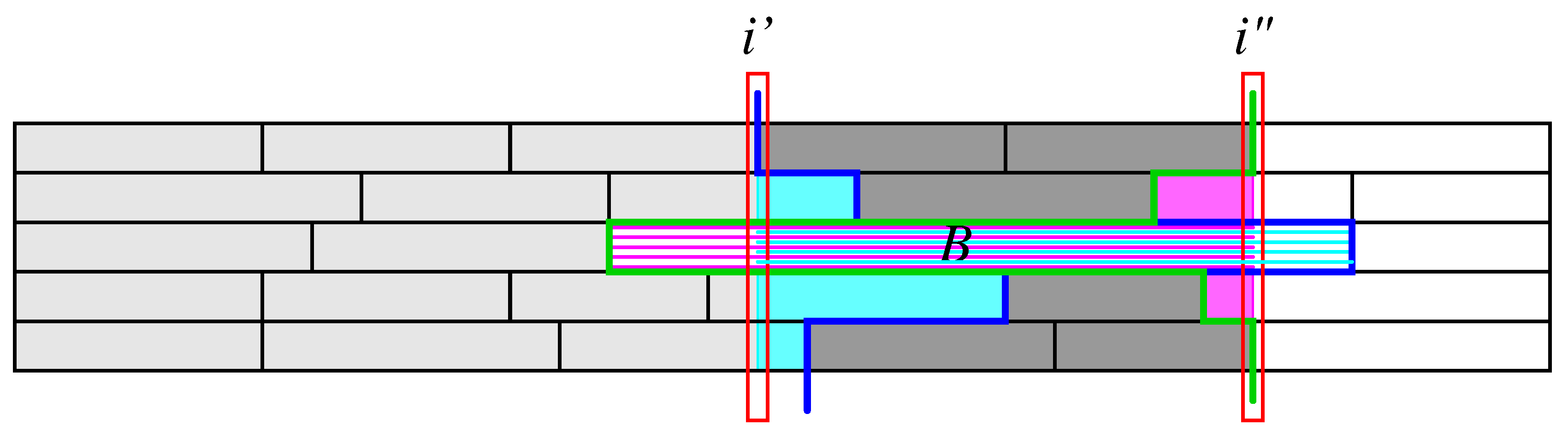
For a given boundary i in , the first term sums all intervals in that do not extend beyond i, while the second sum also includes those that begin before or at i and extend beyond i. Thus, captures all segments of the that are contained within with one important exception: Segments, such as B in Figure 2, that contain contribute to but not to . Such overlapping segments will be taken care of in a correction term discussed below. Using the notation and we, furthermore, define terms
where each sum contains at most a single term, namely the interval that extends across i. Note that intervals that begin or end in position i do not contribute to or , respectively. The correction terms correspond to the parts of segments that are non-trivially intersected by , shown in magenta and cyan, resp., in Figure 2. Thus covers exactly all the intervals contributing to – with the exception of segments that begin at and end at as mentioned above. For such segments, instead of the contributions for and , a single contribution for the interval has to be used. In addition, the contribution for B that is erroneously subtracted with , needs to be restored. Collecting these contributions, we obtain the following correction term for intervals that span across the interval of interest:
For the interval , the correction term defined in Equation (11) can be understood as follows: the first term accounts for the correct contribution of , the second term compensates for the error introduced by , and the remaining two terms remove the superfluous contributions introduced by and . We summarize this derivation in the following form:
Theorem 1.
The potential-dependent segment scores defined in Equation (7) can be expressed as
The only term that depends on both and k is the correction of long input intervals . The restricted sum over the in Equation (11) contains at most one segment for each input segmentation and, thus, can be evaluated in time for a given interval. Furthermore, the sum is certainly empty whenever is larger than the largest segment in any of the ; this can be used to speed up the evaluation from to if the segment lengths in the input are bounded by a constant, except for the short intervals.
Lemma 1.
The arrays of correction terms , , , and can be computed in total time.
Proof.
The values of and can be computed iteratively: we obtain by adding the contribution to whenever for the segmentation . Similarly, is obtained by adding to if . For each i, therefore, we require operations. The sums in Equation (10) comprise at most one segment of for every q. All terms can be computed in constant time using auxiliary arrays that return, for each i and q, the values of and for and . These auxiliary arrays in turn can obviously be constructed in time for the breakpoint list of the input segmentations. □
It, therefore, makes sense to precompute the arrays , , , and .
Corollary 1.
The score can be computed in time with preprocessing cost to compute the arrays , , , and .
It is worth noting, finally, that there is nothing to be gained by storing the score values since each entry is used only once in the recursion.
2.3. Boundaries of Consensus Segments
For a function g on , we define the local curvature at x as . A function g is (strictly) convex at x if . This condition immediately implies that x is not a local maximum of g since at least one of or is larger than . Correspondingly, g is (strictly) concave in x if , whence x is not a local minimum.
Definition 1.
The potential is boundedly convex if satisfied for all intervals
For boundedly convex , the curvature in non-increasing as the intervals become larger. In particular, suppose depends only on the length of the interval and is a smooth function, then and for all implies is boundedly convex.
Theorem 2.
Let be a set of segmentations with union segmentation and suppose is boundedly convex. Then, the consensus is refined by the union segmentation .
Proof.
Following References [24,33], we assume, for contradiction, that the optimal consensus has a segment boundary that is not contained in the union segmentation . We aim to show that moving to some close-by position x will reduce the cost . We focus on a fixed input segmentation and denote by . Denote by and q the first boundaries to the left and to the right of in . Analogously, and are the first boundary to the left and to the right of in , respectively. Thus, contains the two segments and . Since every segment of is a subset of a unique segment of , we have .
We proceed by evaluating how varies when the boundary is perturbed. Let x be the perturbed boundary position. Since only and depends on x and all boundaries except are fixed, it suffices to focus on the intervals and , respectively. Collecting all constant terms in , we obtain
Since is boundedly convex, we have and , whence . Thus, is concave at x for every and, thus, also for any non-negative contribution to the linear combination of input segmentations. Thus, as a function of the moving boundary x cannot have a minimum in the interior of the interval , contradicting the assumption that is a boundary in the optimal consensus . □
Theorem 2 establishes a very useful property: All segment boundaries of the consensus are contained in the union segmentation. This property was observed for disagreement distance and information distance (see below) in the unweighted setting [24,33]. Here, we show it holds for a broader class of distance functions and arbitrary weighting schemes. The techniques used in the proof of Theorem 2 do not seem to generalize to potentials with increasing curvature. Numerical data, however, indicate that the union segmentation refines the consensus for a much larger class of potential functions.
From an algorithmic point of view, it implies that it suffices to compute the for those values of k where segment boundaries are in the union segmentation of the inputs . Correspondingly, we need to store the auxiliary variables only for the intervals of the union segmentation, instead of each i. That is, the recursion (8) reduced to
where denotes the i-th segment boundary in the union segmentation .
Recursion (15) also speeds up the computation of the scoring function , which now is also needed only for the segment boundaries. First, note that we still obtain from by adding the contributions for the intervals ending at the boundary to since by definition and are consecutive breakpoints. Analogously, is obtained by adding for all blocks beginning at to . The terms and remain the same. The correction term could be stored for all pairs of the boundaries in . Alternatively, it suffices to store the m boundaries at which the intervals crossing start and to keep track of the correct correction term directly in recursion (15). Equation (15), thus, can be evaluated in , where s is the number of breakpoints in the union segmentation.
2.4. Length Bounds on Consensus Segments
It is reasonable to expect that a consensus segmentation cannot be a lot coarser than the individual input segmentations. To see that this is indeed the case, we start with a technical observation.
Lemma 2.
Consider intervals , and . Then if for every there is with such that
Proof.
Equation (7) implicitly defined as the term in parentheses, which in turn is the -weighted sum of contributions for each . Consider with . The contribution of to is
Now, consider an alternative segmentation in which A is subdivided into at some position x inside B. Then, A contributes
The terms corresponding to the segments that intersect A are the same as before since either or , depending on whether comes before or after B in . Thus, we have if and only if Equation (16) is satisfied. Since , , and are convex linear combinations of the , , and , respectively, it is sufficient for that holds for all . □
In other words, if A satisfies the condition of Lemma 2, then strictly decreases when A is subdivided into and . Thus, we conclude:
Corollary 2.
An interval A satisfying the conditions specified in Lemma 2 cannot appear in a consensus segmentation.
Our goal is now to show that sufficiently long intervals A always satisfy the conditions of Lemma 2 and, thus, can never be part of the consensus segmentation. Here, we need that is superadditive, i.e., for all and . This is the case particularly for the polynomial potentials. It fails for the negentropy potential, Equation (17), however, because this function is not monotonically increasing with the segment length .
Theorem 3.
Let be a superadditive potential. Let B be the longest segment in the input segmentations and denote by the length of the shortest interval A such that , where and . Then every segment of the consensus segmentation is shorter than .
Proof.
If is superadditive, the l.h.s. of Equation (16) is maximal if (for even ) or for odd , i.e., we assume that x is located in the middle of A. In order to ensure that segments containing x are completely contained in A we need . If this condition is satisfied, Equation (16) applies. We obtain a sufficient condition by replacing the r.h.s. with the maximal possible contribution of the subdivided interval B. By superadditivity, this term monotonically increases with the size of B. The assumption that x equally divides A fixed the l.h.s. of the inequality. Since is strictly superadditive is strictly monotonically increasing with , thus, there is a unique smallest value of unless for all A, in which case no bound exists. □
Corollary 3.
The consensus segmentation with superadditive potential for m input segmentations with length bound as specified in Theorem 3 can be computed in time.
Proof.
We observe that for each k, only values of j between and appear in Equation (8) since longer segments by Theorem 3 cannot be part of an optimal consensus segmentation. The corollary now follows immediately from Corollary 1. □
The length bound on consensus segments, thus, leads to a reduction of the computational efforts. Although in Theorem 3 may be inconvenient to compute for some choices of the potential , we shall see below that a simple, uniform bound can be obtained for an interesting class of potentials.
2.5. Special Potential Functions
Let us now consider plausible distance functions. The disagreement distance between segmentation was introduced in Reference [24] using the potential . A natural generalization is for . We note that a linear potential , i.e., , yields a constant value of because the sum of all segment lengths adds up to n; thus, is independent of the segmentation .
Recall that the entropy of a discrete distribution is defined as . Given a segmentation , we consider the probabilities of randomly picking a point from a segment, i.e., is the relative length of a segment , where n denotes the total length of the segmented genome or time series. The information distance is the symmetrized conditional entropy, which can also be computed as [24,34]. It corresponds to the potential function
given by the negative of the entropy (negentropy) contribution of the interval A.
It has been shown in References [24,33] that the union segmentation refines the unweighted consensus segmentation for both the disagreement distance and the information distance. This result generalizes to the weighted case and the -disagreement distances with .
Corollary 4.
The consensus segmentation is refined by the union segmentation for the disagreement distance, its α generalization with , as well as the information distance.
Proof.
It suffices to show that the potentials are boundedly convex. For the disagreement distance, we have , and we have and ; for , we have and for . For the negentropy, , we have and , where . The scaling by obviously does not affect the signs. □
Is does not seem possible to generalize the result to potentials that grow faster than quadratically.
Let us finally consider the consequence of Theorem 3. Reusing the convexity results above we can replace by where . A short computation then shows that the inequality in Theorem 3 is satisfied for . Since , we have
Corollary 5.
The consensus segmentation of a collection of segmentations with respect to the α-disagreement potentials contains no segment longer than twice the length of the longest input segment.
This allows us immediately to limit the range of the indices in recursion (8) to .
2.6. Generalization: Symmetrized Boundary Mover’s Distance
Equation (7) highlights the fact that the cost function measures, for each segment , how well A conforms to the input segmentations. As noted above, the additive structure of Equation (7) is sufficient to enable minimization by dynamic programming for arbitrary choices of . If we retain the idea of weighted contributions for each input segmentation, we may write , where measures how well the segment A “fits” into the segmentation . As a minimal requirement, for any given interval A, the score must attain its minimum value if the interval A is a segment in . Since two segmentations in general do not have segments or breakpoints in common, measures are required that are more fine-grained than the distinction between identical and distinct segments or breakpoints. , thus, are similar to a measure of overlap, between A and the segments of that are covered by A. Clearly, the potential-based measures can be understood in this manner.
An interesting class of dissimilarities utilizes the distance between break points instead of the lengths of intersections between segments. For a segmentation with segments , , we define and set , i.e., the segments are . By slight abuse of notation, we write , i.e., we now specify a segmentation in terms of its breakpoints. Moreover, we write to mean that s represents a breakpoint in the segmentation .
The “boundary movers distance” was introduced in References [24,33] as
where is some distance function between the positions s and c on . The dissimilarity measure is not symmetric and satisfies whenever is a refinement of . The segmentation aggregation problem that minimizes , therefore, is solved by the union segmentation , while is minimized by the indiscrete segmentation . As noted in References [24,33], these measures, thus, are only useful with additional constraints on the number or size of allowed segments.
The symmetrized version of , however, has attractive properties for our purposes, as we shall see: Clearly, , where and delimit the segment of within which s resides. If or , the contribution vanishes; hence, we can write
This term individually penalizes a segment of for containing boundary points of in its interior. On the other hand, we can rewrite in terms of segments of by simply splitting the contribution of each boundary between the two adjacent segments:
Here, we have used that the lower bounds of the first segments and the upper bounds of the last segments necessarily coincide (they are the boundary of the interval on which our segmentations live); therefore, they do not contribute to the distance. Again, the minima are only taken over two alternative breakpoints of for each given value of or , namely those delimiting the segments of harboring the breakpoints and of the consensus segment. It is not difficult to see that vanishes only if . Furthermore, can be written as a sum of contributions
for each of the segments and each segment of the input segmentations . Clearly, depends only on the input segmentations and the boundary breakpoints and , i.e., an individual segment in the consensus . The segmentation aggregation problem with the symmetrized boundary movers distance, therefore, can again be solved by dynamic programming recursion Equation (8). A more in-depth analysis of this distance function is the subject of ongoing research.
3. Computational Results
3.1. Implementation
The consensus segmentation algorithm is available as an R package consseg, where the dynamic programing recursion is implemented in C++ via Rcpp (≥0.12.18) and RcppXPtrUtils (≥0.1.1) to allow user-defined potential functions. A CRAN package accompanying this contribution will be made available. The development version is available at https://github.com/Bierinformatik/consseg (accessed on 1 December 2020).
The input segmentations are converted into an index returning for each position k the minimum position and the maximum position of the segment containing k. With their help, is obtained by adding to if . Analogously, is computed by adding to whenever . The terms and are evaluated as defined in Equation (10). These computations are interleaved with the evaluation of , Equation (8). Since the expensive part in the algorithm is the evaluation of the segment cost , we avoid their recomputation in the backtracking step by storing instead the values of the segment boundary j that realizes the minimum in Equation (8) for position k. Thus, the last segment of the optimal segmentation on is . Backtracking then proceeds on . The segment boundaries of the optimal segmentation are, therefore, obtained as , starting from and continuing until is reached. It is worth noting that the fast, incremental Equation (12) is prone to rounding errors for large n and very fast-growing potentials due to the computation of difference of two sums.
3.2. Consensus Segmentation of Yeast Transcriptome Data
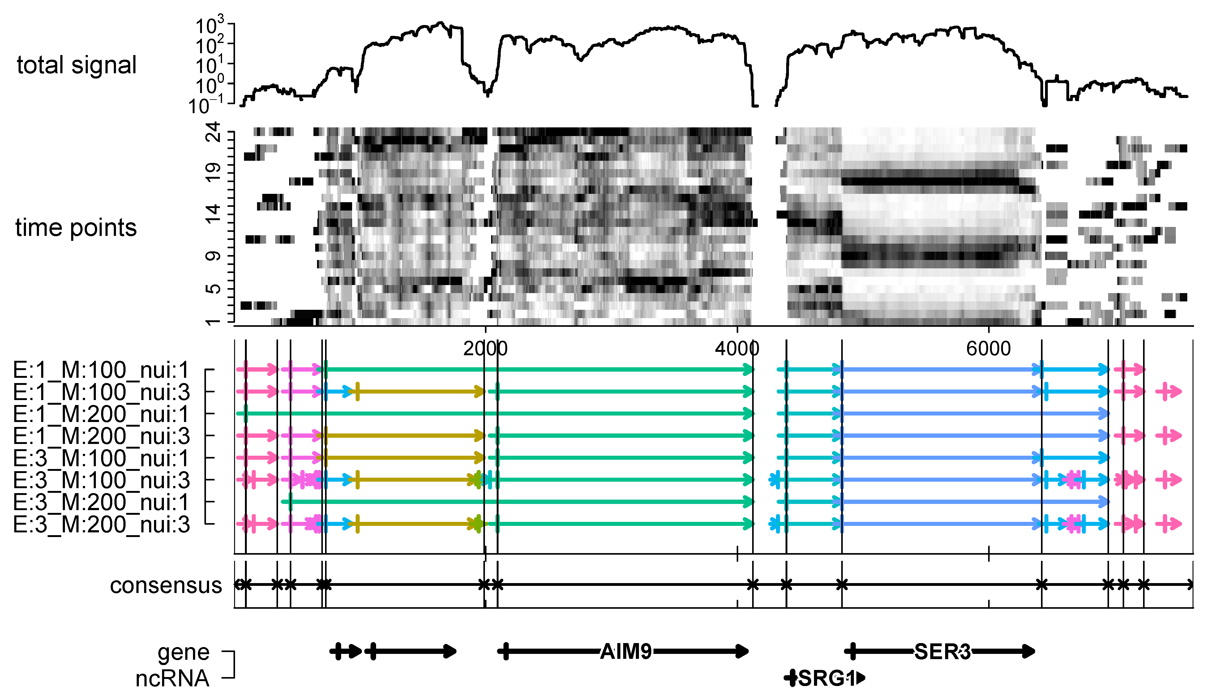
To demonstrate the usefulness of consensus segmentations, we explored the yeast transcriptome time series mentioned in the introduction. We computed the consensus of segmentations obtained with widely different parameter choices [11]. We found that the consensus segmentation appears to produce a robust representation of the transcriptome and seems to fit better to the current annotation of the yeast genome than any particular choice of segmentation parameters. The example in Figure 3 also shows that distinct non-coding components, such as SRG1, are readily detectable. Short segments with very low coverage are likely gaps between transcriptome units without relevant RNA products. Consistently detectable elements, even if lowly expressed, on the other hand, may be of interest for closer inspection.
In order to evaluate the usefulness of consensus segmentations in a more quantitative manner, we quantify the overlap of segments with annotated coding sequences. To this end, we determine for each CDS C the segment with the largest Jaccard index and then record the ratio of segment length and annotation length. In symbols:
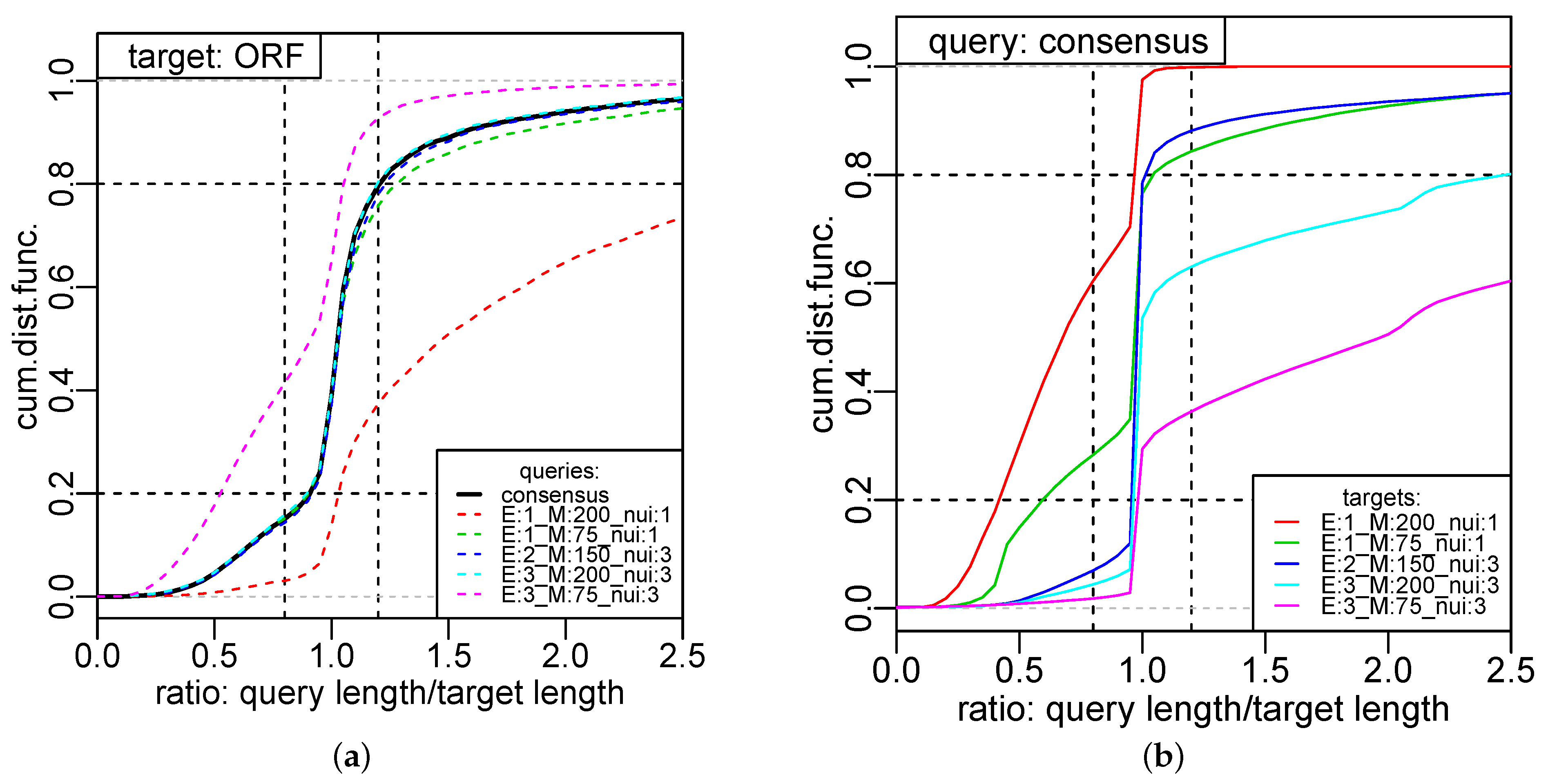
The cumulative distribution function computed over a large set of known transcripts C quantifies the congruence between segmentation and annotation. As a reference we use here the transcripts harboring coding sequences annotated in Reference [36]. A perfect overlap between a consensus segment and the annotated transcript is indicated by , indicates a segment that is shorter and a segment that is longer then the annotated transcript. Figure 4a shows the cumulative distribution function for the 5171 CDSs of S. cerevisae IFO 0233 for five segmentations with widely different parameters computed with segmenTier [11]. The red curve is the consensus over these segmentations. It shows that the consensus segmentation is a robust method: computed from a small sample of distinct segmentations, some of which do not perform particularly well, it performs at least as well as the best individual segmentation obtained from an extensive search of the parameter space in Reference [11]. Discrepancies between annotation and consensus are not only limitations on the segmentation approach but also derive from inaccuracies of the annotation, processing of transcripts, and the complexity of the yeast transcriptome, which harbors abundant overlapping and polycistronic transcripts [37]. The consensus performs as well as the best individual segmentation (according to the benchmark in Reference [11]). Figure 4b shows that the individual segmentations share between about 30% and 70% of the segments with the consensus (corresponding to the height of the vertical jump at ), i.e., the consensus does not simply recapitulate any individual input segmentation. We, therefore, advocate to use the consensus segmentation as a robust and essentially parameter insensitive method for transcriptome analysis in compact genomes.
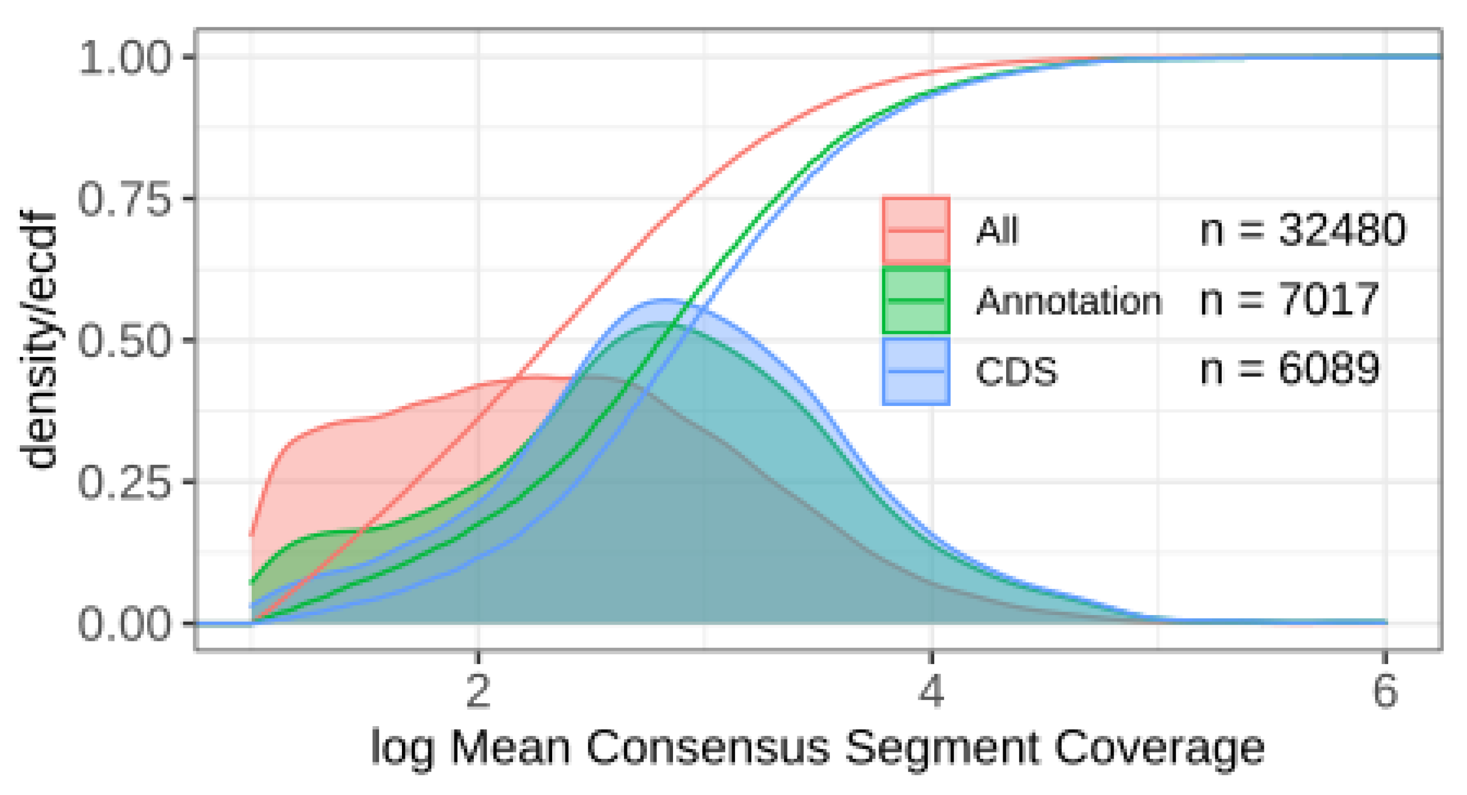
The consensus segmentation of the transcriptome of S. cerevisae IFO 0233 comprises 74,091 segments. After filtering for spacers using the input segmentations [11] and very short segments that most likely correspond to small overlaps and noise in the RNA-seq data, we retained 32,480 segments. Figure 5 shows the distribution of median coverage. Not surprisingly, segments overlapping known protein-coding sequences (CDS) show higher expression levels than other segments. Many segments overlap various types of long non-coding RNAs, such as CUTs and SUTs [38,39]. We also observe many segments with substantial expression levels that so far have remained unannotated, providing a large pool of candidates for novel ncRNAs. Transcriptome segmentation is only the first step towards an accurate and reliable genome annotation. The subsequent processing of the segmentation data, however, is beyond the scope of this present contribution and will be addressed in forthcoming work.
3.3. Consensus Segmentations of Growth Curves
The usefulness of consensus segmentations is by no means limited to transcriptome data or segmentations of genomes. We, therefore, include here also a very different application. The growth of a population of bacteria over time can be quantified by measuring the apparent absorption, usually referred to as OD (optical density), in a spectrophotometer. Growth curves typically show distinct growth regimes: an initial time lag that precedes a phase of exponential growth, which is followed by a deceleration phase that finally settles into saturation, see, e.g., Reference [40]. These can be separated by approximating the time course of by a sequence of line segments, i.e., as a continuous, piece-wise linear function. The corresponding approximation problem is again a segmentation problem that can be solved by dynamic programming [28]. Empirically, one observes that resulting segmentations are quite sensitive to small difference in the growth curves. We show here that the consensus segmentation is a convenient way to extract a robust estimate for the duration of the different phases.
In Figure 6, we compare the growth curves of four Escherichia coli cultures grown in minimal glucose medium at 37 C. The R package dpseg [41] was used to segment the individual growth curves. This package also uses a dynamic programming approach. Instead of fixing the number of segments as in Reference [28], it uses a penalty parameter to adjust the resolution of the segmentation. Considering the consensus of the individual segmentations and the variation of the breakpoints across the replicates provides a more realistic view of that data compared to the segmentation of an averaged growth curve.
3.4. Refinement Conjecture
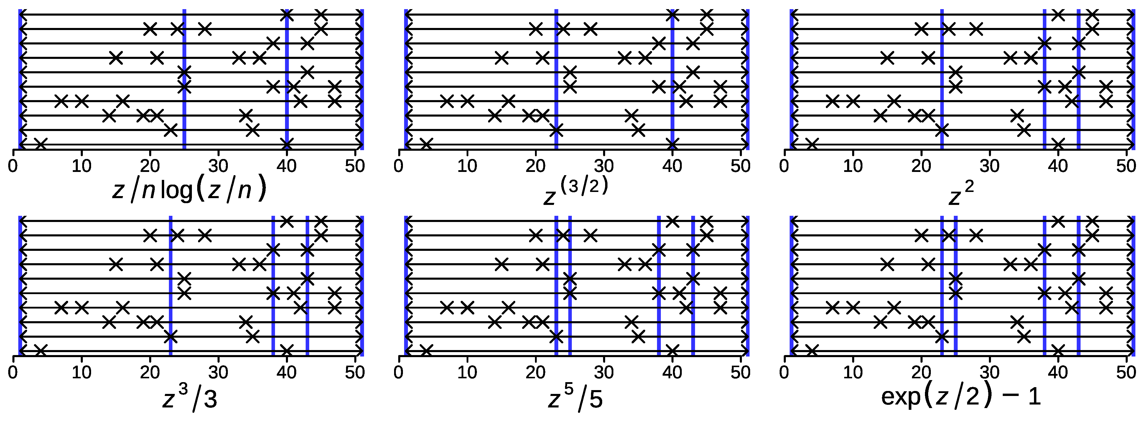
Theorem 2 states that the union segmentation refines the consensus segmentation for the class of boundedly convex consensus functions. Numerical simulations strongly suggest that this is true also for many potentials with increasing positive curvature, despite the failure of the proof technique for the general case. We simulated 10 segmentations of length 50 and a maximum of 10 segments, using the base-R sample function to randomly choose breakpoints in a given range. Figure 7 shows consensus segmentations for six potential functions from negentropy to exponential.
We found that the consensus segmentation only contained breakpoints that are present in at least one of the input segmentation. This suggests:
Conjecture 1.
appears to refine for all superadditive potentials and possibly even for all convex potentials.
This “Refinement Conjecture” is of considerable practical use. If true, (assumed as a heuristic), it reduces the computational effort to where s is the number of break points in the input segmentations. We further observed a trend for faster-growing potentials to yield more and, thus, shorter consensus segments. This is consistent with the fact that the bound on the length of the consensus intervals in the argument leading up Corollary 5 decreases with the exponent in polynomial potentials.
4. Concluding Remarks
In this work, we have extended and generalized previous work [24,33] on the segmentation aggregation problem. We showed that for the class of boundedly convex potential functions, including negentropies and powers with , all consensus breakpoints are breakpoints in at least one of the contributing segmentations. Furthermore, we showed that for all superadditive potentials, consensus segments cannot be longer than twice the longest input segment. This bound allows a further reduction of the computational effort.
Consensus segmentations as described here pertain to two major application scenarios: (i) Reconciliation of segmentations of multi-dimensional data, comprising, e.g., independent measurements, such as biological or technical replicates, or measurements of different quantities, e.g., different histone modifications. (ii) Reconciliation of segmentations of the same data set produced with different similarity measures. In principle, it is also possible to compute the consensus segmentation of different segmentations produced, e.g., with randomized algorithms or different heuristics using the same similarity measures. A major advantage of consensus segmentations is that they can be computed without specific information about the data underlying the input segmentations. Such knowledge is not needed because the segmentation aggregation problem depends only on the distance function D as a “parameter”. Empirically, we found that variations of the distance functions have only very moderate consequence on the consensus segmentation.
In simulations, we found strong support for the Refinement Conjecture. This provides support for approaches that utilize a dynamic programming segmentation method to select be best segmentation from the union of segmentations that are computed with different heuristics. Such a scheme has been proposed in Reference [42]. In this manner, one can potentially achieve a substantial gain in computational efficiency compared to the full dynamic programming segmentation. The C-KS approach [12] also restricts itself to the union segmentation.
We considered two very different application scenarios. In applications to transcriptome data consensus segmentations have the potential to substantially improve annotations. A particular strength of the consensus approach is, by highlighting differences that are consistent between data tracks, the ability to identify processing-related boundaries. This is of particular interest in organisms with operons, poly-cistronic primary transcripts, or no expression-free gaps between genes. In all these cases, it becomes difficult and often impossible to distinguish transcriptional units from patterns of mapped RNA-seq reads alone. Here, we have used data from yeast strain IFO 0233, which has been used previously to illustrate transcriptome segmentation in Reference [11]. We have seen that the consensus segmentation provides a robust prediction of transcriptomic units from a moderate number of individual segmentations with very different parameters. We obtained thousands of segments that may correspond to the non-coding transcripts in S. cerevisae IFO 0233. Since the present contribution is intended to describe the method of consensus segmentation and its mathematical justification, we will report elsewhere on a comprehensive analysis of the IFO 0233 transcriptome.
Consensus formation is also of use to aggregate data from biological replicates. As an example, we showed that consensus segmentations of growth curves can be used to robustly determine distinct growth phases.
The consensus segmentation methods incorporate weights that refer to input segmentations. This feature can be used, for instance, to weight individual transcriptome data by coverage. In the case of growth functions, weights may be chosen to decrease with average measurement error, quantified, e.g., as average deviation from the linear fit. It would also be of interest to associate weights with individual segments. This can certainly be done in the context of the Boundary Mover’s distance. Whether this can be also be achieved in the potential-based approach, and to what extent the mathematics results of this contribution will remain intact, however, is a question for future research.
We observed that consensus segmentations are quite robust w.r.t. to the choice of the potential on real data, while we observed a trend towards shorter consensus segments with increasing for the power potentials on i.i.d. random data. Conceptually, consensus segmentations based on the comparison of segments are designed to handle essentially arbitrary heterogeneity along the time or genome coordinate, while breakpoint-centered approaches, such as C-KS, need to rely on statistical regularities of true breakpoints. In order to assess the utility of different potentials and dissimilarity measures , and to compare the segment-centered dynamic programming approach with breakpoint-centered alternatives, a principled way of benchmarking consensus segmentation methods will be necessary. This will require, in particular, the development of a simulator for correlated segmentations that mimic characteristics of different types of underlying data. At present, such tools are not available.
Our analysis of consensus segmentations suggests several avenues for future research. From a theoretical point of view, the most immediate open problem is the Refinement Conjecture, and the characterization of the potential function and—more generally—the dissimilarity measures for which the union segmentation refines the consensus segmentation. This is also of practical relevance since the recursions can be restricted to breakpoints of the union segmentation in such cases; see Equation (15). In addition, a more detailed understanding of the consensus segmentation would be useful. For instance, are there potentials or dissimilarities that guarantee a breakpoint in the consensus within every interval that contains a breakpoint in every input segmentation, or in the (weighted) majority of the input segmentations? Such results could immediately be used to limit the scope of j in Equation (8). More generally, one may ask whether the idea of consensus segmentation can give rise to useful ways of measuring the local accuracy or reliability of consensus and/or input break points.
Author Contributions
All authors jointly contributed the conceptualization of the study, the theoretical results, the interpretation of the results, and the writing of the manuscript. All authors have read and agreed to the published version of the manuscript.
Funding
This work was supported in part by the German Federal Ministry for Education and Research (BMBF 031A538B as part of de.NBI and BMBF 031L0164C, RNAProNet, to P.F.S.), the Deutsche Forschungsgemeinschaft (DFG proj. nos. AX 84/4-1 and STA 850/30-1), and the Lebanese Association for Scientific Research (LASeR). H.S. receives a Landesgraduiertenstipendium of the Free State of Saxony.
Institutional Review Board Statement
Not applicable.
Informed Consent Statement
Not applicable.
Data Availability Statement
The RNA-seq data for the example in Figure 1 and Figure 3 (SRG1 ncRNA and SER3 protein coding gene) is available via the segmenTier R package (object tsd can be loaded with data(primseg436)) and the bacterial growth curves in Figure 6 via the dpseg package (oddata is available after loading the package). The genome-wide RNA-seq data will be made available at a public repository with a full report on the data (in progress, work by RM, PFS and DBM). The segmentations of the yeast IFO 0233 transcriptomes are available as Supplemental File in csv format.
Conflicts of Interest
The authors declare no conflict of interest. The funders had no role in the scientific content of this work.
Abbreviations
| CDS | Coding sequence |
| CUT | Cryptic unstable transcript |
| ncRNA | non-coding RNA |
| SGD | Saccharomyces Genome Database |
| SUT | Stable uncharacterized transcripts |
| ORF | Open reading frame |
| i.i.d. | independent and identically distributed |
| Glossary of mathematical symbols: | |
| Segments in a segmentation | |
| Interval of from to i to j (inclusive) | |
| Consensus segmentation (of a set of segmentations) | |
| (Input) segmentation | |
| Weight of an input segmentation | |
| Union segmentation (of a set of segmentations) | |
| Distance (dissimilarity) between segmentations | |
| Boundary movers distance | |
| Score of a partial segmentation on | |
| Potential of an interval | |
| Score on a consensus interval | |
| Score contribution of segments ending no later than i | |
| Score contribution of segments beginning no later than i | |
| Score contribution of r.h.s. part a segment spanning i | |
| Score contribution of l.h.s. part a segment spanning i | |
| score correction for segments beginning before i and ending after j | |
References
- Pirooznia, M.; Goes, F.S.; Zandi, P.P. Whole-genome CNV analysis: Advances in computational approaches. Front. Genet. 2015, 6, 138. [Google Scholar] [CrossRef] [Green Version]
- Yen, A.; Kellis, M. Systematic chromatin state comparison of epigenomes associated with diverse properties including sex and tissue type. Nat. Commun. 2015, 6, 7973. [Google Scholar] [CrossRef]
- Zeller, G.; Henz, S.R.; Laubinger, S.; Weigel, D.G.R. Transcript Normalization and Segmentation of Tiling Array Data. Pac. Symp. Biocomput. 2008, 13, 527–538. [Google Scholar]
- Hardcastle, T.J.; Kelly, K.A.; Baulcombe, D.C. Identifying small interfering RNA loci from high-throughput sequencing data. Bioinformatics 2012, 28, 457–463. [Google Scholar] [CrossRef] [PubMed] [Green Version]
- Bischler, T.; Kopf, M.; Voß, B. Transcript mapping based on dRNA-seq data. BMC Bioinform. 2014, 15, 122. [Google Scholar] [CrossRef] [PubMed] [Green Version]
- David, L.; Huber, W.; Granovskaia, M.; Toedling, J.; Palm, C.J.; Bofkin, L.; Jones, T.; Davis, R.W.; Steinmetz, L.M. A high-resolution map of transcription in the yeast genome. Proc. Natl. Acad. Sci. USA 2006, 103, 5320–5325. [Google Scholar] [CrossRef] [Green Version]
- Danford, T.; Dowell, R.; Agarwala, S.; Grisafi, P.; Fink, G.; Gifford, D. Discovering regulatory overlapping RNA transcripts. J. Comput. Biol. 2011, 18, 295–303. [Google Scholar] [CrossRef] [PubMed] [Green Version]
- Braun, J.V.; Müller, H.G. Statistical methods for DNA sequence segmentation. Stat. Sci. 1998, 13, 142–162. [Google Scholar] [CrossRef]
- Elhaik, E.; Graur, D.; Josić, K. Comparative Testing of DNA Segmentation Algorithms Using Benchmark Simulations. Mol. Biol. Evol. 2010, 27, 1015–1024. [Google Scholar] [CrossRef]
- Girimurugan, S.B.; Liu, Y.; Lung, P.Y.; Vera, D.L.; Dennis, J.H.; Bass, H.W.; Zhang, J. iSeg: An efficient algorithm for segmentation of genomic and epigenomic data. BMC Bioinform. 2018, 19, 131. [Google Scholar] [CrossRef] [Green Version]
- Machné, R.; Murray, D.B.; Stadler, P.F. Similarity-Based Segmentation of Multi-Dimensional Signals. Sci. Rep. 2017, 7, 12355. [Google Scholar] [CrossRef] [PubMed] [Green Version]
- Toloşi, L.; Theißen, J.; Halachev, K.; Hero, B.; Berthold, F.; Lengauer, T. A method for finding consensus breakpoints in the cancer genome from copy number data. Bioinformatics 2013, 29, 1793–1800. [Google Scholar] [CrossRef] [PubMed] [Green Version]
- Segal, M.R.; Wiemels, J.L. Clustering of Translocation Breakpoints. J. Am. Stat. Assoc. 2002, 97, 66–76. [Google Scholar] [CrossRef] [Green Version]
- Rand, W.M. Objective criteria for the evaluation of clustering methods. J. Am. Stat. Assoc. 1971, 66, 846–850. [Google Scholar] [CrossRef]
- Fowlkes, E.B.; Mallows, C.L. A method for comparing two hierarchical clusterings. J. Am. Stat. Assoc. 1983, 78, 553–569. [Google Scholar] [CrossRef]
- Ben-Hur, A.; Elisseeff, A.; Guyon, I. A stability based method for discovering structure in clustered data. Pac. Symp. Biocomput. 2002, 7, 6–17. [Google Scholar]
- Hubert, L.; Arabie, P. Comparing partitions. J. Classif. 1985, 2, 193–218. [Google Scholar] [CrossRef]
- Mirkin, B. Mathematical Classification and Clustering; Kluwer Academic Press: Dordrecht, The Netherlands, 1996. [Google Scholar]
- Van Dongen, S. Performance Criteria for Graph Clustering and Markov Cluster Experiments; Technical Report; Centrum voor Wiskunde en Informatica: Amsterdam, The Netherlands, 2000. [Google Scholar]
- Mirkin, B.G. On the Problem of Reconciling Partitions. In Quantitative Sociology: International Perspectives on Mathematical and Statistical Modeling; Blalock, H.M., Aganbegian, A., Borodkin, F.M., Boudon, R., Capecchi, V., Eds.; Academic Press: New York, NY, USA, 1975; pp. 441–449. [Google Scholar]
- Barthélemy, J.; Leclerc, B. The median procedure for partitions. In Partitioning Data Sets; Cox, I., Hansen, P., Julesz, B., Eds.; American Mathematical Society: Providence, RI, USA, 1995; Volume 19, pp. 3–34. [Google Scholar] [CrossRef]
- Křivánek, M.; Morávek, J. NP-hard problems in hierarchical-tree clustering. Acta Inform. 1986, 23, 311–323. [Google Scholar] [CrossRef]
- Wakabayashi, Y. The complexity of computing medians of relations. Resenhas IME-USP 1998, 3, 323–349. [Google Scholar]
- Mielikäinen, T.; Terzi, E.; Tsaparas, P. Aggregating Time Partitions. In Proceedings of the 12th ACM SIGKDD International Conference on Knowledge Discovery and Data Mining; Eliassi-Rad, T., Ungar, L., Craven, M., Gunopulos, D., Eds.; Association for Computing Machinery: New York, NY, USA, 2006; pp. 347–356. [Google Scholar] [CrossRef]
- Meilă, M. Comparing Clusterings: An Axiomatic View. In Machine Learning, Proceedings of the Twenty-Second International Conference; De Raedt, L., Wrobel, S., Eds.; Association for Computing Machinery: New York, NY, USA, 2005; pp. 577–584. [Google Scholar] [CrossRef]
- Meilă, M. Comparing clusterings by the variation of information. In Learning Theory and Kernel Machines; Schölkopf, B., Warmuth, M.K., Eds.; Springer: Berlin/Heidelberg, Germany, 2003; Volume 2777, pp. 173–187. [Google Scholar] [CrossRef]
- Vingron, M.; Sibbald, P.R. Weighting in sequence space: A comparison of methods in terms of generlized sequences. Proc. Natl. Acad. Sci. USA 1993, 90, 8777–8781. [Google Scholar] [CrossRef] [PubMed] [Green Version]
- Bellman, R. On the approximation of curves by line segments using dynamic programming. Commun. ACM 1961, 4, 284–286. [Google Scholar] [CrossRef]
- Bai, J.; Perron, P. Computation and analysis of multiple structural change models. J. Appl. Econom. 2002, 18, 1–22. [Google Scholar] [CrossRef] [Green Version]
- Fragkou, P.; Petridis, V.; Kehagias, A. A Dynamic Programming Algorithm for Linear Text Segmentation. J. Intell. Inf. Syst. 2004, 23, 179–197. [Google Scholar] [CrossRef]
- Picard, F.; Robin, S.; Lavielle, M.; Vaisse, C.; Daudin, J. A statistical approach for CGH microarray data analysis. BMC Bioinform. 2005, 6, 27. [Google Scholar] [CrossRef] [Green Version]
- Huber, W.; Toedling, J.; Steinmetz, L.M. Transcript mapping with high-density oligonucleotide tiling arrays. Bioinformatics 2006, 22, 1963–1970. [Google Scholar] [CrossRef] [PubMed] [Green Version]
- Terzi, E. Problems and Algorithms for Sequence Segmentations. Ph.D. Thesis, Department of Computer Science Series of Publications A Report A-2006-5, University of Helsinki, Helsinki, Finland, 2006. [Google Scholar]
- Haiminen, N.H.; Mannila, H.; Terzi, E. Comparing segmentations by applying randomization techniques. BMC Bioinform. 2007, 8, 171. [Google Scholar] [CrossRef] [PubMed] [Green Version]
- Martens, J.A.; Laprade, L.; Winston, F. Intergenic transcription is required to repress the Saccharomyces cerevisiae SER3 gene. Nature 2004, 429, 571–574. [Google Scholar] [CrossRef]
- Xu, Z.; Wei, W.; Gagneur, J.; Perocchi, F.; Clauder-Munster, S.; Camblong, J.; Guffanti, E.; Stutz, F.; Huber, W.; Steinmetz, L.M. Bidirectional promoters generate pervasive transcription in yeast. Nature 2009, 457, 1033–1037. [Google Scholar] [CrossRef]
- Pelechano, V.; Wei, W.; Steinmetz, L.M. Extensive transcriptional heterogeneity revealed by isoform profiling. Nature 2013, 497, 127–131. [Google Scholar] [CrossRef] [PubMed] [Green Version]
- Parker, S.; Fraczek, M.G.; Wu, J.; Shamsah, S.; Manousaki, A.; Dungrattanalert, K.; de Almeida, R.A.; Invernizzi, E.; Burgis, T.; Omara, W.; et al. Large-scale profiling of noncoding RNA function in yeast. PLoS Genet. 2018, 14, e1007253. [Google Scholar] [CrossRef] [Green Version]
- Till, P.; Mach, R.L.; Mach-Aigner, A.R. A current view on long noncoding RNAs in yeast and filamentous fungi. Appl. Microbiol. Biotech. 2018, 102, 7319–7331. [Google Scholar] [CrossRef] [PubMed] [Green Version]
- Hall, B.G.; Acar, H.; Nandipati, A.; Barlow, M. Growth Rates Made Easy. Mol. Biol. Evol. 2014, 31, 232–238. [Google Scholar] [CrossRef] [PubMed] [Green Version]
- Machné, R.; Stadler, P.F. dpseg: Piecewise Linear Segmentation by Dynamic Programming. R Package Version 0.1.2. 2020. Available online: https://cran.r-project.org/web/packages/dpseg/ (accessed on 1 December 2020).
- Pierre-Jean, M.; Rigaill, G.; Neuvial, P. Performance evaluation of DNA copy number segmentation methods. Brief. Bioinform. 2015, 16, 600–615. [Google Scholar] [CrossRef] [PubMed] [Green Version]
Figure 1.
Segmentation of RNA expression patterns. Top: RNA expression in 24 samples taken every 4 min from Saccharomyces cerevisae strain IFO 0233 (shown as color scale, with the total of all experiments shown above). The sequencing data are strand-specific, only the plus strand of about 5000 nt on chromosome V are shown. Middle: nine different segmentations computed with segmenTier using different parameter settings; see Reference [11] for details on data and segmentations. Below: annotated coding and non-coding yeast genes. The rightmost block of short segments is a candidate for an unannotated ncRNA located anti-sense to the much longer protein-coding gene Utp7p on the minus strand. The data are the same as those in Figure 3 of Reference [11].

Figure 2.
Definition of auxiliary variables. The input segments contributing to are all those to the left of the green line (i.e., the ones shown in light and dark gray. are to the left of the blue line, i.e, those shown in light gray. The large interval B is included in but not in . The correction terms and comprise the cyan and magenta parts, respectively. The correction term , finally adds takes care of the interval B.

Figure 3.
Alternative segmentations of the yeast transcriptome data shown in Figure 1 (here, the coverage time-series is shown as gray-values and the logarithms of the total coverage). Below, we show eight alternative segmentations computed with segmenTier [11] with different parameter settings. The consensus segments, computed for potential , match very well with the expectations from visual inspection of the data and from the annotation of yeast the genome (bottom). SRG1 is a non-coding RNA that represses the adjacent SER3 gene by transcriptional interference [35].

Figure 4.
Quantitative evaluation of the consensus of genome-wide transcriptome segmentations of RNA-seq data from S. cerevisae from ref. [11]. (a) Cumulative distribution function of the length ratios r between overlapping segments and previously annotated ORF transcripts [36]. A ratio of indicates a good match. The consensus (black solid line) of five representative segmentations (colored dashed lines) by segmenTier with widely different parameter settings (as indicated in Figure 2d of Reference [11]) is at least on par with the best individual segmentation. (b) Overlap of the consensus with the five different input segmentations. The individual segmentations share between about 30% and 70% of their segments with the consensus (vertical jump at ). The consensus was computed with .

Figure 5.
Distribution of RNA expression across the consensus segmentation of S. cerevisae IFO 0233. We distinguish segments that overlap a coding sequence (CDS) or another annotation item (Annotation) present in the current genome annotation taken from SGD (Saccharomyces Genome Database), and unannotated segments (All). An overlap of at least 30% with an annotation item was required. Densities are normalized to 1 for each class. Cumulative distributions are superimposed.

Figure 6.
Four Escherichia coli cultures were grown at identical conditions (four replicates in a larger experiment) in M9 medium with 0.2% glucose at 37 C in a BMG Clariostar platereader and the optical density at 600 nm, was measured every 10 minutes. The growth curves of each of the four replicates were segmented into intervals with constant slope by the dpseg algorithm with the default jump penalty parameter [41].

Figure 7.
Consensus segmentation (shown by blue vertical lines) for a collection of 10 random segmentations with equal weights for six different potential functions . Note that only breakpoints of the input segmentations (marked by × appear in the consensus segmentation.
Figure 7.
Consensus segmentation (shown by blue vertical lines) for a collection of 10 random segmentations with equal weights for six different potential functions . Note that only breakpoints of the input segmentations (marked by × appear in the consensus segmentation.

Publisher’s Note: MDPI stays neutral with regard to jurisdictional claims in published maps and institutional affiliations. |
© 2021 by the authors. Licensee MDPI, Basel, Switzerland. This article is an open access article distributed under the terms and conditions of the Creative Commons Attribution (CC BY) license (http://creativecommons.org/licenses/by/4.0/).
Share and Cite
MDPI and ACS Style
Saker, H.; Machné, R.; Fallmann, J.; Murray, D.B.; Shahin, A.M.; Stadler, P.F. Weighted Consensus Segmentations. Computation 2021, 9, 17. https://0-doi-org.brum.beds.ac.uk/10.3390/computation9020017
AMA Style
Saker H, Machné R, Fallmann J, Murray DB, Shahin AM, Stadler PF. Weighted Consensus Segmentations. Computation. 2021; 9(2):17. https://0-doi-org.brum.beds.ac.uk/10.3390/computation9020017
Chicago/Turabian StyleSaker, Halima, Rainer Machné, Jörg Fallmann, Douglas B. Murray, Ahmad M. Shahin, and Peter F. Stadler. 2021. "Weighted Consensus Segmentations" Computation 9, no. 2: 17. https://0-doi-org.brum.beds.ac.uk/10.3390/computation9020017
Note that from the first issue of 2016, this journal uses article numbers instead of page numbers. See further details here.