
Least-Squares Finite Element Method for a Meso-Scale Model of the Spread of COVID-19


Department of Computational Mathematics, Humboldt-Universität zu Berlin, 12489 Berlin, Germany
*
Author to whom correspondence should be addressed.
Computation 2021, 9(2), 18; https://0-doi-org.brum.beds.ac.uk/10.3390/computation9020018
Submission received: 15 December 2020
/
Revised: 19 January 2021
/
Accepted: 28 January 2021
/
Published: 5 February 2021
(This article belongs to the Special Issue Computation to Fight SARS-CoV-2 (CoVid-19))
Abstract
:This paper investigates numerical properties of a flux-based finite element method for the discretization of a SEIQRD (susceptible-exposed-infected-quarantined-recovered-deceased) model for the spread of COVID-19. The model is largely based on the SEIRD (susceptible-exposed-infected-recovered-deceased) models developed in recent works, with additional extension by a quarantined compartment of the living population and the resulting first-order system of coupled PDEs is solved by a Least-Squares meso-scale method. We incorporate several data on political measures for the containment of the spread gathered during the course of the year 2020 and develop an indicator that influences the predictions calculated by the method. The numerical experiments conducted show a promising accuracy of predictions of the space-time behavior of the virus compared to the real disease spreading data.
1. Introduction
The outbreak of the global pandemic caused by the novel virus responsible for COVID-19 had, and still has, a great impact on the life of the global human population. Human lives are threatened greatly by this highly infectious virus with higher probability of death and long-term damages to individuals of higher age or with a compromised immune system. Due to this delicate situation of global influence, various political measures have to be taken to prevent the virus from spreading as much as possible before an effective vaccine can be developed and distributed among the population to ensure immunity of a substantial part of the population that eventually causes the virus to die out. The most prominent question in the meantime, however, is that of the measures to be taken to ‘flatten the curve’ of new infections as the virus seems to spread exponentially if exposure is not regulated in any way. Among the measures already taken by the governments are curfews, lockdowns of whole cities and countries, quarantines of people exposed to the virus or that recently have been to areas with a high impact, travel restrictions, and—most commonly propagated measure on social media—social-distancing. But, to this point, there does not seem to be a general (political) consensus about the safest plan to slow the spread of the virus and which measures are the most effective, imposed on the people in exactly which level of strictness. This calls for a scientific modeling of the epidemiological behavior of this virus to form a plausible foundation for regulations. Such a model needs to extract some patterns thereof from the scattered data collected during the time of first notice in late 2019 until the latest developments today and to convert them into functions that can effectively predict new developments in the future. Regulating factors, such as exposure and mortality rates, can hopefully be witnessed and then, in turn, used to optimize the political measures accordingly.
The well-known epidemiological models of SIR type (susceptible-infected-recovered) have been extensively analyzed, and we refer to Reference [1] for an overview. This model works with a separation of the general population that needs to be studied into certain compartments (S, I, R) that have different roles in the spread of and affection by the virus and have a different use in the respective models. This compartment list can be extended to account for the further specifications of the disease, and we refer to Reference [2] for an overview. For example, the SEIR model includes an exposed group and the SEIRD (susceptible-exposed-infected-recovered-deceased) model separates truly recovered and deceased. The choice of these compartments for COVID-19 modeling has been the subject of many recent publications. The experts in modeling seem to agree that a COVID-19 model should account for asymptomatic transmission and that a quarantined group might be relevant (see Reference [3,4,5,6,7,8,9]).
A further challenge is the modeling of the spatial spread of the epidemic diseases in geographical regions. Several works, therefore, coupled the classical SIR model with inter-city networks, as in Reference [10,11]. To this aim, the classical epidemiological models of SIR type have been recast in the variational setting of analytical mechanics in Reference [12] with continuum partial differential equation models with diffusion terms describing the spatial variation in epidemics. First, mechanical and mathematical investigations in this direction were pursued in Reference [13,14] and seem very promising. A derivation of such a coupled system of PDEs without particular reference to an established SIR model has been conducted in Reference [15], where the authors have shown how the epidemiological dynamics can be expressed in PDEs step-by-step. For a mathematical analysis of a similar SIR model, we refer to Reference [16]. Another link can be drawn to the field of machine learning, as neural network predictors have proven themselves recently in similar fields, such as traffic and social modeling. Deep learning structures have been used to develop predictors for the COVID-19 virus spread. The techniques of using training data to be fed to the neural network that automatically computes a possible prediction are a great advantage in comparison to classical FEM methods that need a detailed model and a system of PDEs thought-out beforehand. A work on this forecast of the regional spread and intensity of the virus prevalence is presented in Reference [17]. Limitations, however, are exactly these training data, or the lack thereof, as at the beginning of the pandemic there might have not been a big enough variety of data to train the algorithm properly, and this can be linked to a choice of which data to use to make a most fitting prediction, until newer case numbers and their distribution are known.
In this work, we opted for a continuum partial differential equation model as in Reference [13,14] but added the quarantined compartment. Moreover, instead of a classical variational formulation, an approximation of the solution is obtained with a mixed formulation involving the fluxes of the variable accounting for the number of individuals in each group. This variational formulation is chosen to be of Least-Squares type, such that the linearization is relatively straightforward, the solving procedure involves a positive definite matrix, and we can use the inherent error estimator for adaptive strategies. We will map out the country of Germany with respect to accumulating regions and incorporate the ideas of travel restrictions and contact limitations imposed on the population. A further advantage of this approach is that it will give us the possibility to account for the political interventions made by the government in a hope to contain the spread of the virus in affected areas. To give an analysis of the spread of the virus under the already existing imposed political measures, data on restrictions, such as travel and contact reduction or bans, have been studied in the example of Germany. During early stages of the virus development in Europe, the case counts in this country have been significantly smaller than the ones of the neighboring countries. As respective measures of regulation have been taken early-on in March and April with rising numbers and a successful containment of the spread was achieved due to fast decreasing new daily infection rates, this serves as an indicator that the political decisions taken could have been effective. Another aspect is the division of the country in individual states, similar to the USA, with their own respective government that could more or less individually regulate the graveness of the measures, while the state intervened with German-wide restrictions only a few times during the time period of March until November. Such federal “infection containment acts” have been imposed, for example, during the lockdown in March with rather strict almost-curfew measures and then the permission to the individual states of relaxation of these acts, e.g., of the contact restrictions from single-household contacts to two-household rules or small groups and then successive enlargement of the number of people allowed at public gatherings or festivities. Eventually, the “lockdown light” has been re-inforced following the alarming high numbers of new daily infections. The indication as “light” is a terminology chosen by the government to contrast the “regular” lockdown in March that had stricter regulations imposed on businesses and catering that caused the economy to recess slightly.
We aimed at presenting a solution technique to the system of PDEs constructed by the SEIQRD (susceptible-exposed-infected-quarantined-recovered-deceased) model using a Least-Squares Method to predict the regional spread of COVID-19 in the country of Germany. We rely on data gathered by the Federal Statistical Office of Germany on actual numbers of infections, the reduction of incoming and outgoing flights, and contact restrictions as political reactions to contain the spread. These data serve to develop an indicator that is a key part in our calculations and shows at which time containment regulations gripped and give rise to a likely decrease (or increase) in subsequent new numbers of infections and their regional spread. Interpolation is used to fit and avoid losses of data and the resulting predicted versus real-life data will be presented in order to show the applicability of our Least-Squares solution method. To this end, this paper is structured subsequently in 5 more sections. In Section 2, the SEIQRD model is stated, and, in Section 3, the Least-Squares Method and the resulting first-order system to be solved are discussed. Following this, we develop the special discretization of the system in Section 4 and focus on the explanation of the parameters and their fitting using our indicator in Section 5. The numerical results are presented and analyzed in Section 6.
2. Model
We opt to change the usual SEIRD (susceptible-exposed-infected-recovered-deceased) model for epidemiological studies to a SEIQRD model that also takes into account a quarantined compartment of the population infected with the virus.
This model assumes that the living population is divided into five compartments: the susceptible population , the exposed population , the infected population , the recovered population , the quarantined population , and deceased population . As in the works of Reference [13,14], we do not consider the birth rate nor the general (non-COVID-19) mortality rate and denote with the sum of the living population, i.e.,
with the functions representing the respective compartments for convenience of formulating the coupled PDE model. Note that, since we consider the compartment D of the deceased population, n does not vary over the time.
We distinguish between recovery rates , contact rates , the inverse of the incubation period , a backflow , and the quarantining rate .
Following Reference [13], we denote by the asymptomatic recovery rate and recall that it is the proportion of change in the exposed group that never enters the infected group (as they stay undetected) towards the recovered group. In the sense of the subsequent notations, that means that there is a decrease in the number of exposed people and an increase of recovered people.
Similarly, denotes the infected recovery rate, i.e., the infected people that do show symptoms and, therefore, enter the regulated process of quarantine as an intermediate step (see below) before entering the recovered population.
is the inverse of the incubation period that indicates how fast exposed individuals change to infected individuals after known exposure to the virus.
One particularity of the new virus is that as of now the status of immunity of recovered patients is unclear. Therefore, we opt for a model that assumes that not all recovered patients are immune; thus, the backflow is included that carries the proportion of recovered patients that are not immune back to the susceptible individuals with rate .
We now want to consider the additional effect of the quarantine and choose a quarantine scheme connected to the infected, exposed and recovered, as a natural way to symbolize that quarantined people can be both in a state of yet non-discovered infection, being asymptomatic, healthy, or symptomatic (which means visibly showing symptoms that a possible infection with the virus might be accounted for). This quarantine rate should change with time and based on political decisions, as it has been mandatory for returnees from highly affected areas to undergo self-quarantine for several days while waiting for the result of the test that indicates the infection status. Quarantined individuals can recover or decease, as seen below.
Moreover, we follow the thoughts of Reference [10] and make the deceased linearly dependant on the quarantine, as the death of these individuals is connected to a visible infection that needs treatment in medical facilities that impose a strict quarantine on these patients. Thus, we get
with the fatality rate .
In order to model the tendency of outbreaks to cluster towards large population centers, we follow the idea of Reference [13] and consider the Allee effect, which, in a sense, defines a correlation between the density of a population and the fitness of its individuals, with constant parameter . We, therefore, need to consider the partial derivatives in space and introduce the space of weak derivatives on a simply connected geographical domain . For sufficiently smooth, the Allee effect now reads
with
where is the contact rate at which the exposed asymptomatic patients transmit the virus to susceptible individuals, and is the symptomatic contact rate.
Note that, in order to simplify the notation, we skipped the time dependence in the notation of the coefficients. However, those coefficients are supposed to change over time, as we will see in Section 5.
3. The Least-Squares Method
The class of Least-Squares Finite Element Methods is based on the idea of the residual minimization of a variational problem and as these methods rely on inner-product projections, they tend to be particularly robust and stable. While traditional finite element methods are usually developed from a variational setting that comes almost directly from the problem to solve at hand, Least-Squares Methods work exactly the other way round by fixing a variational framework before and then fitting the problem into this framework. For an introduction to this class of numerical methods, we refer the reader to Reference [22].
With the notation , , , , as well as
the system can be written in a vector form as
for and with our time interval of interest. Defining leads to
The components of then belong to the space of integrable divergence, i.e.,
where a Neumann boundary condition g on the boundary of is prescribed in the space. With and the matrix
we obtain
Using an implicit Euler time discretization, the first-order system reads
Our Least-Squares Finite Element method consists of the least squares minimization of in , which means we search
for all . As the function f is a nonlinear function of , we will solve with the Gauss–Newton Multilevel Method proposed in Reference [23]. In fact, the main theorem states that if an iterative method is used which converges uniformly with respect to h, then a stopping criterion of the form
based on a particular residual is useful with independent of h. Here, this residual is defined as the scalar product
with the Fréchet derivative of (omitting the notation of dependence on the data of the previous step) in the direction in the discretization space (to be defined in Section 4 below) that we calculate in the following. As the nonlinearity is concentrated in the term , we introduce
in order to simplify the notation. The variable is not to be confused with , as indicates the time step performed by the Euler discretization in the Gauss-Newton Multilevel Method in Reference [23].
For the derivative associated with the variable , we obtain
and, for the linear part associated with the variable , we have
For the directional derivatives of the function f, we first state
such that
and, with the matrix K and the notation from before, we obtain
4. Finite Element Discretization
In this work, we considered a fixed time step , while space-time adaptivity will be considered in a follow-up paper. Therefore, in each time-step, the finite element discretization of the Least-Squares Finite Element Method consists of considering the minimization problem (19) in a finite-dimensional subspace , based on a triangulation of , i.e., we search in , satisfying
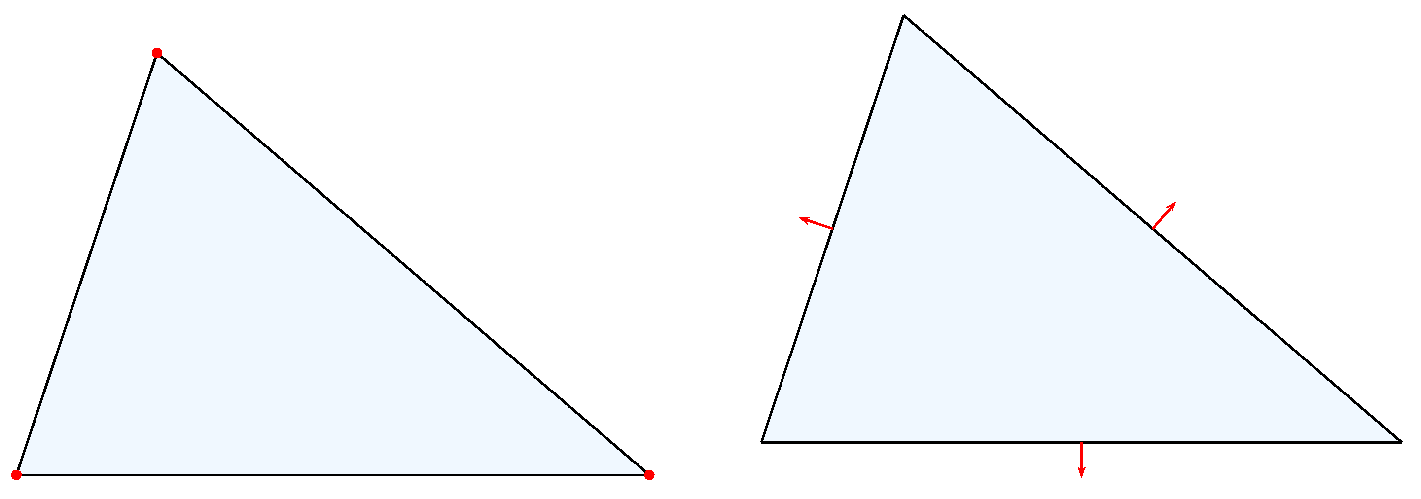
for all . As the Least-Squares Method does not require any compatibility of the finite element spaces, we choose as the standard Lagrange element and the Raviart-Thomas element space accounting for the Neumann boundary condition prescribed by the function g. The Raviart-Thomas spaces for arbitrary degree k and dimension n of the are defined as
where is the space of local polynomials of degree at most k on a triangle . For the case , , this gives
The local degrees of freedom of the combination are pictured in Figure 2.
The inner basis functions of can be defined on the edge-path , where and are the adjacent triangles of the edge E by the following formula:
Such a basis function is shown in Figure 3. With our computations of the Fréchet derivative, the nonlinear least-squares problem (33) is equivalent to the variational problem
for all .
This is a nonlinear algebraic least-squares problem which we solved using an inexact Gauss-Newton method similar to the one presented in Reference [23]. Successive approximations to the nonlinear least-squares problem are, therefore, obtained by minimizing the linear least-squares problem
Recall that minimizing in is equivalent to the variational formulation
for all . Following the suggestion of the authors, we use
as stopping criterion, i.e., the Gauss-Newton iteration is stopped as soon as the nonlinear residual satisfies (20), where we choose . The steps are summarized in Algorithm 1.
| Algorithm 1: Gauss-Newton for minimization of the nonlinear functional. |
 |
5. Parameter Fitting
This section is devoted to the description of the parameters that are used in the PDEs (11a)–(11e). The key idea is that we assume is linearly dependent on some indicator taking into account the political measures. Surely, the linear dependency is an important restriction and nonlinear functions will be considered in a follow-up paper. On the other side, the SIR-type models are based on a linear incidence rate such that this ansatz is expected to give first adequate results. We also let vary over the time, taking into account that the health system had to learn and to increase the capacities. does not vary in space. We started with an ansatz corresponding to a polynomial of degree 5, and it turned out that a polynomial of degree 3 is sufficient.
The other parameters are assumed not to be dependent on the political restriction and, therefore, are constant in time.
For the design of this indicator, we took inspiration from the flight data found in Reference [24] for the comparison to the numbers of the COVID-19 not-yet inflicted year 2019 in Germany and the flight reduction in the year 2020 taken from Reference [25]. This data has been collected by the Statistisches Bundesamt (Federal Statistical Office of Germany) and is publicly accessible.
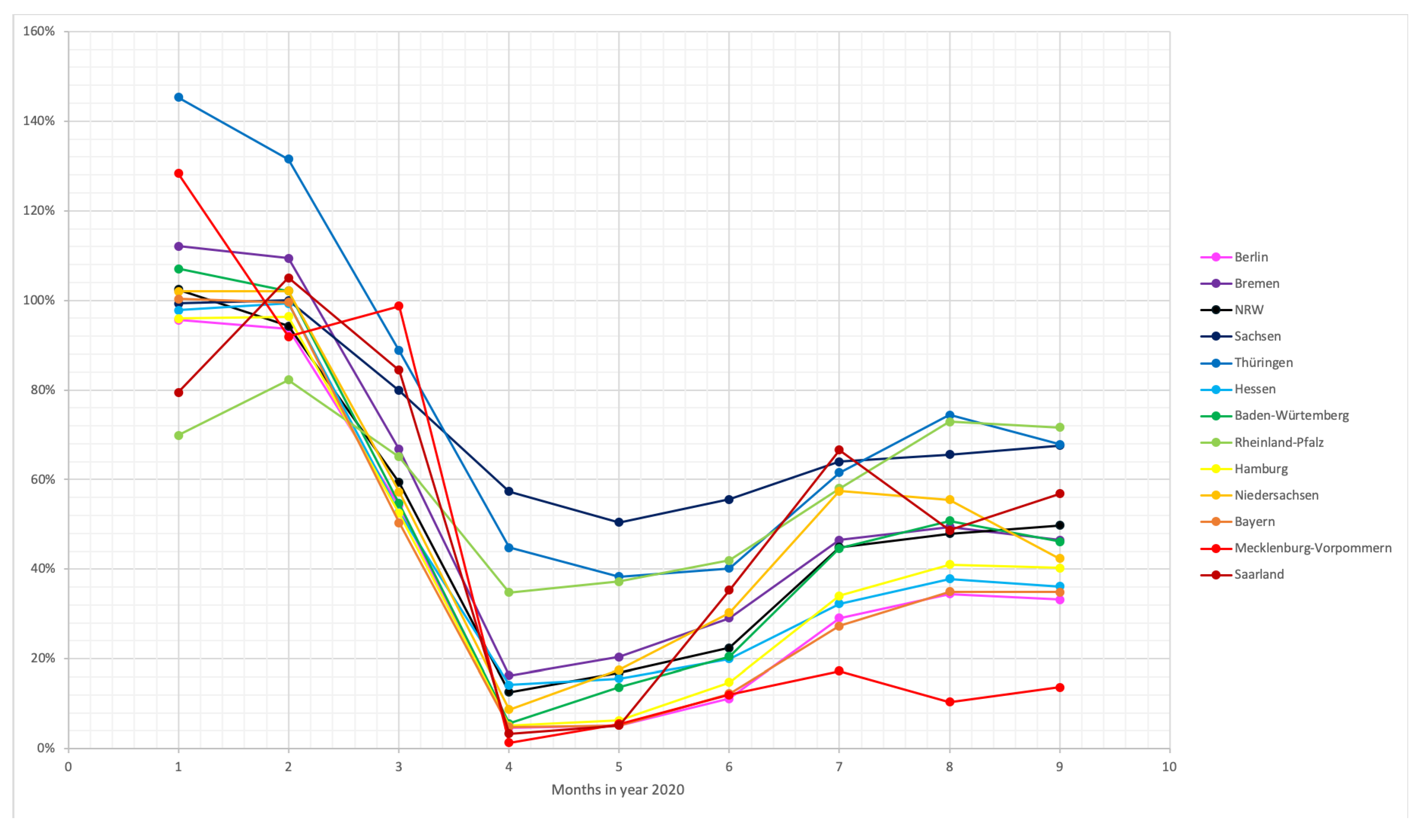
The indicator follows the data gathered for the reduction of the number of outgoing and incoming flights, as well as the contact reduction measures imposed by the government, over the time period of the outbreak of COVID-19 in Germany dating from January (or March, as the contact restraints haven been imposed later) until September 2020. The assumption that justifies this indicator is a correlation of the measures and the intensity of virus prevalence within the population. Our model is fed by two aspects, the first being the reduction of flights. This is based on the fact that following the growing international numbers in January, the government took measures of reducing flights to contain the risk of the residential population to be infected by travelling individuals that might come back from a high-risk area. This also gives rise to the question of reasonable initial values for the indicator and draws a connection between these of the compartments presented earlier in Section 2. Figure 4 shows how drastically the number in flights decreases up to April and then slowly increases again but stagnates in August.
This can be linked to our second class of data, the contact restrictions. As the numbers in infections surged in March, a lockdown was announced across Germany with the same regulation imposed in every federal state: Only people belonging from their own household could be met and maximum one other person in public. Big gatherings have been forbidden completely and even travelling restrictions across the federal states (within the country!) have been imposed via bans on touristic stays at hotels. A model that takes these travel restrictions into account has also been considered in Reference [26]. These restrictions have been successively loosened on a private and a public level over the course of May and June and in July, August, and September the situation has been lead towards further normalization by permissions for public gatherings with growing numbers of participants of 100, 200, 350, etc. This tendency is reflected in the flight numbers, as they have been increasing from the depression in April, while being still far away from pre-pandemic numbers. The differences in the states can be seen while studying the respective “infection containment acts” and press releases (given that the numbers are reflected correctly). Not all states, however, have completely discarded the contact restraints in June and July (like Brandenburg and Mecklenburg-Vorpommern) but stayed with a moderate permission to meet an arbitrary number of people belonging to two households or a group of maximum 10 people from different households (like in Bavaria). These, however, are regulations for public meetings, but private gatherings have frequently not been observed, or no regulations have been imposed on private premises whatsoever (Bavaria, since June).
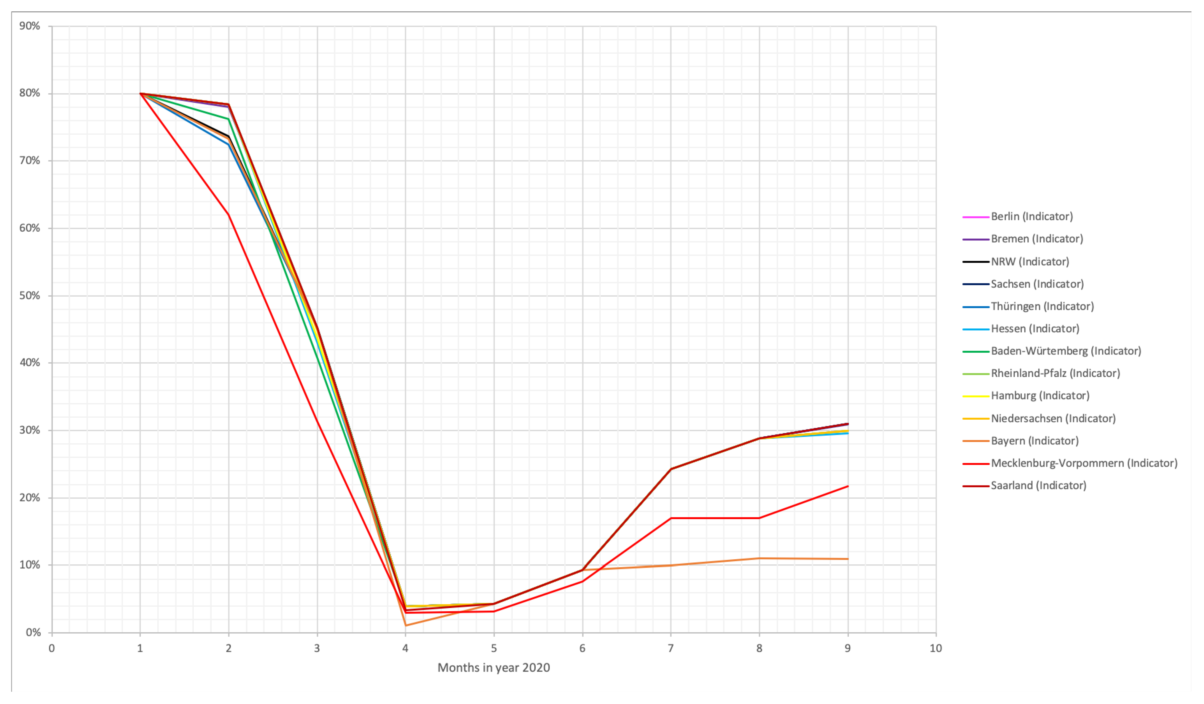
Drawing together these two classes of data we developed an indicator, the numbers of which can be seen in Table 1 and Figure 5. The indicator combines the contact limitations and the travel restrictions in terms of flights to create a weighting in the sense that the spread of the virus in already existing infections stays more close-region bound and the number of new infections is predicted to stay lower than an uncontrollable development without any restrictions. Thus, a value of 0.8, for example, indicates that due to travel and contact restrictions active at that time, a reduction of the transmission rates of the virus in our model towards 80% is used in the calculations compared to the uncontrolled case. At the beginning of 2020, restrictions for flights from China were already in place, as well as limitations of large events. Therefore, we chose to set this indicator to 0.8 for January in all federal states. Depending on how fast the government of the respective state were in implementing the measures, we let this indicator decrease until April. Note, for instance, that Bavaria had the strictest regulation in April and has, therefore, the smaller indicator in April. Similarly, the regulations were decreasing in July but remain very strong, and this is the reason why this state has, again, the smallest indicator from July to September.
6. Numerical Experiment
We performed the numerical experiment with the open source FENICS (see, e.g., Reference [27]). We use a finite-element spatial discretization of Germany, consisting of an unstructured mesh containing 1773 elements. Further results with finer meshes and adaptive mesh refinement strategies will be presented in a follow-up paper. In this project, we restricted ourselves to the time step day due to the fact the the coupled PDE had to be solved many times. The initial conditions are the data from the “COVID-19 Dashboard” [28] of the Robert Koch-Institut (see Supplemental Materials), the leading epidemiological research institute in Germany concerned with data gathering at this time, of February 15th in which evaluations are based on the reporting data transmitted from the health authorities according to IfSG (infection protection acts). Data can be individually chosen for the respective states and regions. On the coast part of the German border, zero Neumann boundary conditions are set, while, on the remaining part, the data from an SRI model without diffusion (nor quarantine) are used.
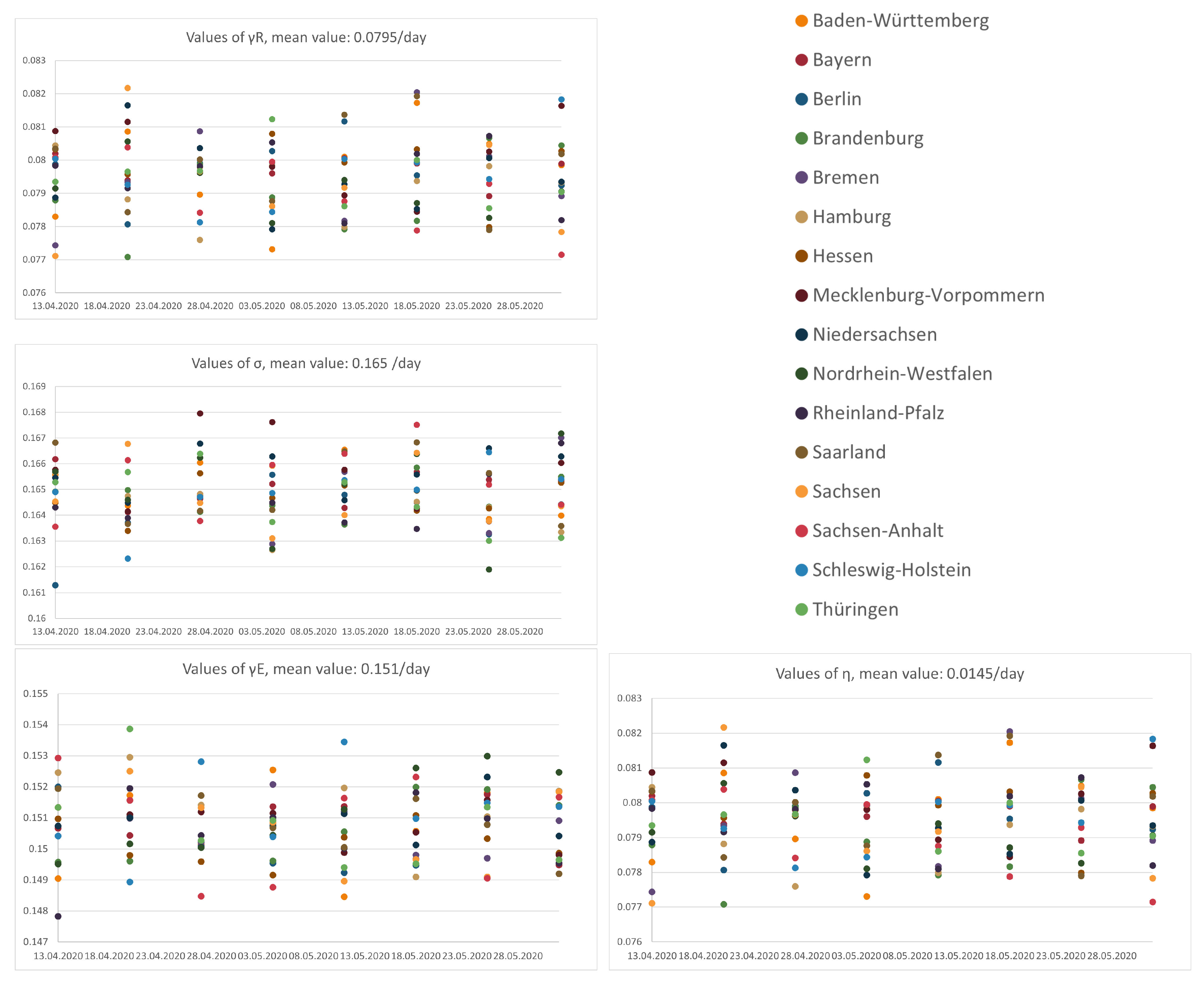
The data from 15th February to 1st June was used for the calibration for the constant-in-time parameters, i.e., . In order to investigate the sensibility of these coefficients, we also reproduced the calibration using less data, always starting from 15th February. For each Bundesland (federal state), we show the results in Figure 6. For the parameter depending on the indicator, the results of this analysis are shown in Figure 7. Figure 8 shows the evolving spatial pattern of the COVID-19 outbreak in Germany. A comparison of the prediction and the data from RKI is shown in Figure 9.
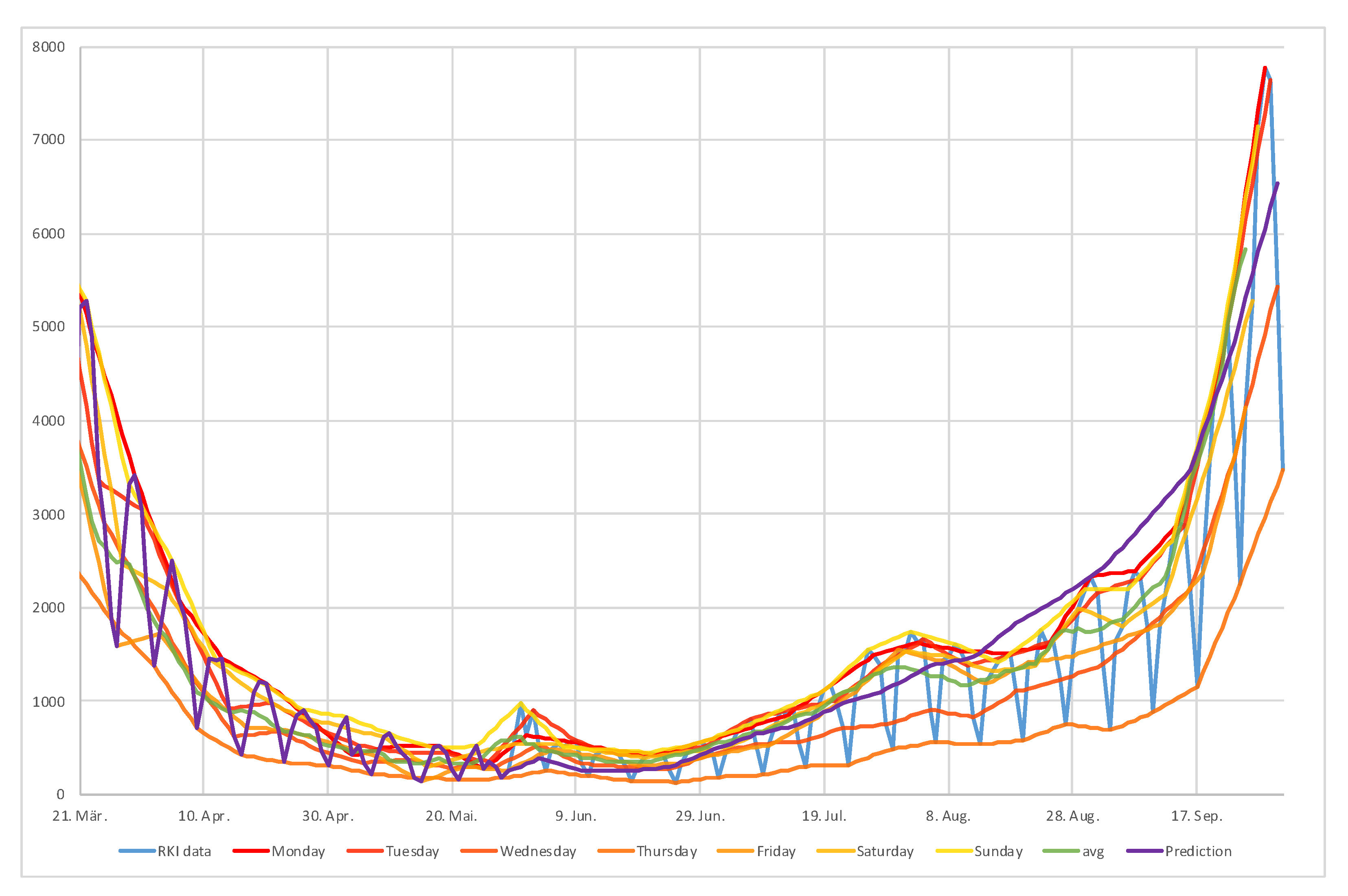
In order to present an evaluation of the accuracy of the prediction we start by considering the error as the forecast minus the real RKI data. Unfortunately, the RKI data are not monotone due to infrastructural and organizational reasons. For instance, reported new infections are linked to the days of the week in a sense that the public health departments are frequently closed over the weekends and have only started to register new cases also during the weekends after the situation has been severely more tense. Thus, Monday reports contain more new cases than the other days of the week up until Friday, as it can also contain the cases to be accounted towards Saturday and Sunday.
From the RKI data, we, therefore, constructed a piecewise linear interpolation with
between each weekday, as well as the average of the last seven days. The difference between the RKI data and these interpolations, as well as the difference between the RKI data and the prediction, are shown in Figure 10. We see that the prediction overshoots the Thursday line, such that the error is positive.The forecast undershoots none of the other lines over the whole prediction time. We note that, until the beginning of August, the forecast undershoots the line and the error is negative. After this time, the forecast overshoots all the RKI interpolations until the end of September. The different errors are shown in Figure 11. We remark that the error oscillates taking into account that the RKI data oscillates. Overall, the error remains smaller than the error due to the piecewise linear interpolation of the data.
In order to deal with these discrepancies, we computed the mean absolute percentage error (MAPE) and root-mean-square error (RMSE) for each of the previously mentioned interpolations of the RKI data. These quantities, obtained with
are given in Table 2. These can be compared to the numbers in the work [10] to find a similar accuracy of the prognostic. We remark, again, that the interpolation has a larger effect:
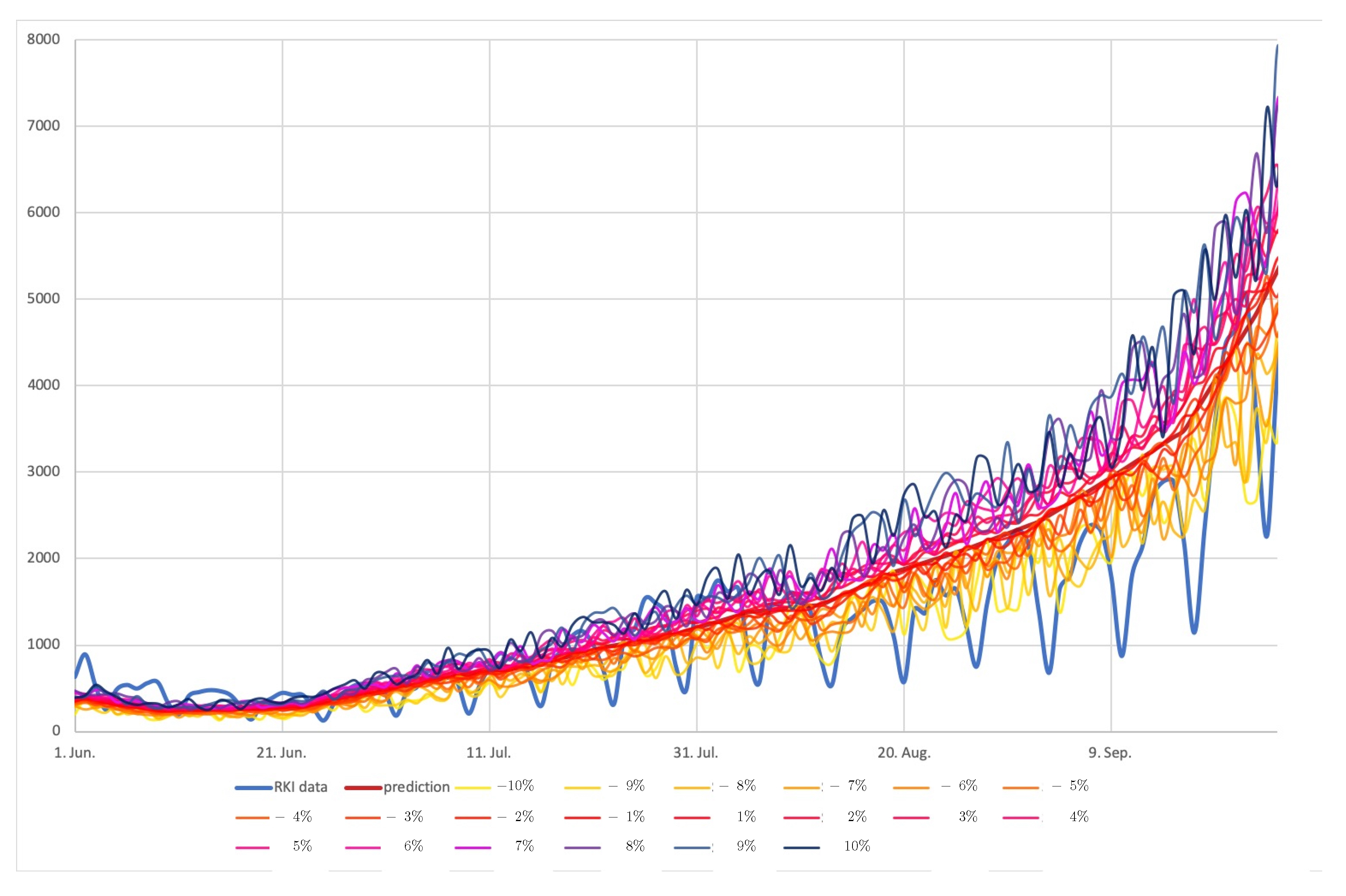
In order to study how the model is sensitive to the indicator, we perturbed the indicator up to . The results in Figure 12 indicate that small variations are acceptable, as the resulting data stay all in a close proximity, even so still in a reasonable range in the second half of the timeline.
While the results of our numerical experiments look very promising, this is definitely to be accounted to some of the specific decisions we took for tailoring our calculations. For the indicator, we had to set a suitable initial value, for example, which represents the percentage of non-restrictions (100% means no restrictions) at some point. In addition, while the data we collected are a lot, only certain moments where incorporated and it is also always unknown beforehand whether the contact restrictions, for instance, will always be followed directly after press announcement. In this sense, the human choice is a big factor that cannot always be considered accordingly. (We refer to the most recent developments, as a “hard lockdown” has been imposed at the beginning of November that is still active, but the count of new infection cases per day have not decreased to a “satisfactory level” since. One of the reasons could be the dissatisfaction of large parts of the population with the deemed too drastic and restrictive measures, calls for demonstrations and large (and also private) gatherings without proper regard of the distancing measures, the loosening of the rules during Christmas-time, and the like.)
Our employed model is largely based on the works of Reference [10,13,14] and our Least-Squares solution technique shows a consistency with the numerical results presented in these works. However, some adjustments have been made in order to fit the computational work more tightly to the real-life data, thus producing more promising predictions. In Reference [13], the model successively forecasts exposed and infected cases which at this point are of high importance to the public health institutions. Similarly to our interpolation technique, a comparison of an “optimistic” and a “pessimistic” case can be witnessed, with the actual real-life data lying in between. Like the authors of this work, we come to the conclusion that this particular system of PDEs successively models the local virus dynamics on a meso-scale level.
The question of interest for practical relevance of our work remains: Can the predictions be used to influence and support political decisions in terms of virus containment? The answer is yes, but the transmission dynamics have to be investigated more closely in order to limit grave effects (like lockdowns) on the whole of the population. It could be more favorable to single out so-called virus hubs and rather focus on containment strategies in these areas while maintaining a tolerable, moderate policy for the remaining areas. To this end, the authors of Reference [10] present a detailed work on inter-state transmission that can be accounted to the use of the GLEAM network that serves to analyze the dynamics more closely in heavily-affected regions due to tourism and high traffic density. In addition, concrete rates for specific contact restrictions (that also include, for example, school closings, which could be one of the new aspects that we could include, as well in future work) have been used in the model, while we rely on the indicator for parameter fitting. It has to be noted though that the problem of limited testing and the related dark figures arises, that introduces a uncertainty in the data that is used for parameter calibration. Nevertheless, the use of such a network in our model could lead to even more closely fitted spacial predictions of spread and, thus, more detailed timelines, like in Figure 8, where, in part (f), some suggested virus hubs are noticeable of the type that the authors of Reference [10] can predict very accurately with the fine-tuning of the GLEAM network. Like in our approach, the predictions never undershot the actual observed numbers (in the most relevant cases), which indicated a high potential in practical use.
In Reference [14], another approach is shown that uses a machine learning technique to simulate the spread of the virus. A Bayesian learning in OPAL (Occam Plausibility Algorithm) is presented, where the simulation process in terms of more automatically computing spatio-temporal evolving can be seen. Comparing the resulting correlation and Pearson coefficients, our results show a similar accuracy, presenting two solution techniques to such systems of PDEs. Reference [10] presents a mixture of these two suitable techniques via a meso-scale approach, like ours, and refinement via a machine learning technique, the GLEAM network.
Overall, we observe that our sensitivity analysis suggests that our indicator serves as a good tool to tune our predictions taking into account political measures that are taken. These predictions can in turn be used to help politicians and public health offices to take according measures in terms of contact restrictions and medical, as well as supply resource re-evaluation, to limit the virus spread to a tolerable amount and to anticipate spreads in particularly affected areas due to, for example, touristic location.
For future work, we are considering a more refined tailoring of our discretization method. A more technically challenging task due to its complexity and amount of data it produces is to implement the successive solution of the system with more than one Euler time step in one solution procedure. For further theoretical work, we will try to develop more modifications to classical models in the literature to test the limits of the accuracy of our discretization method. Works in actual simulation will be aimed at, as well.
Supplementary Materials
The following is available at https://0-www-mdpi-com.brum.beds.ac.uk/2079-3197/9/2/18/s1, Table S1: RKI data.
Author Contributions
Both authors contributed equally. Both authors have read and agreed to the published version of the manuscript.
Funding
This research received no external funding.
Data Availability Statement
The data presented in this study are available in the supplemental material provided.
Conflicts of Interest
The authors declare no conflict of interest.
References
- Hethcote, H.W. The Mathematics of Infectious Diseases. Siam Rev. 2000, 42, 599–653. [Google Scholar] [CrossRef] [Green Version]
- Pastor-Satorras, R.; Castellano, C.; Mieghem, P.V.; Vespignani, A. Epidemic processes in complex networks. Rev. Mod. Phys. 2015, 87, 925. [Google Scholar] [CrossRef] [Green Version]
- He, S.; Peng, Y.; Sun, K. SEIR modeling of the COVID-19 and its dynamics. Nonlinear Dyn. 2020, 101, 1667–1680. [Google Scholar] [CrossRef] [PubMed]
- Maier, B.; Brockmann, D. Effective containment explains subexponential growth in recent confirmed COVID-19 cases in China. Science 2020, 368, 742–746. [Google Scholar] [CrossRef] [PubMed] [Green Version]
- Pedersen, M.; Meneghini, M.G. Quantifying undetected COVID-19 cases and effects of containment measures in Italy. ResearchGate Preprint. Available online: https://www.researchgate.net/profile/Morten_Pedersen2/publication/339915690_Quantifying_undetected_COVID-19_cases_and_effects_of_containment_measures_in_Italy_Predicting_phase_2_dynamics/links/5e76433ea6fdcccd62159b49/Quantifying-undetected-COVID-19-cases-and-effects-of-containment-measures-in-Italy-Predicting-phase-2-dynamics.pdf (accessed on 21 March 2020).
- Peirlinck, M.; Costabal, F.; Linka, K.; Kuhl, E. Outbreak dynamics of COVID-19 in China and the United States. Biomech. Model. Mechanobiol. 2020, 27, 1–15. [Google Scholar] [CrossRef]
- Kucharski, A.J.; Russell, T.W.; Diamond, C.; Liu, Y.; Edmunds, J.; Funk, S.; Flasche, S. Early dynamics of transmission and control of COVID- 19: A mathematical modelling study. Lancet Infect. Dis. 2020, 20, 553–558. [Google Scholar] [CrossRef] [Green Version]
- Jia, J.; Ding, J.; Liu, S.; Liao, G.; Li, J.; Duan, B.; Wang, G.; Zhang, R. Modeling the Control of COVID-19: Impact of Policy Interventions and Meteorological Factors. arXiv 2020, arXiv:2003.02985. [Google Scholar]
- Yongzhen, P.; Shaoying, L.; Shujing, G.; Shuping, L.; Changguo, L. A delayed SEIQR epidemic model with pulse vaccination and the quarantine measure. Comput. Math. Appl. 2009, 58, 135–145. [Google Scholar] [CrossRef] [Green Version]
- Kergaßner, A.; Burkhardt, C.; Lippold, D.; Kergaßner, M.; Pflug, L.; Budday, D.; Steinmann, P.; Budday, S. Memory-based meso-scale modeling of Covid-19-County-resolved timelines in Germany. Comput. Mech. 2020, 66, 1069–1079. [Google Scholar] [CrossRef]
- Lu, Z.; Yu, Y.; Chen, Y.; Ren, G.; Xu, C.; Wang, S.; Yin, Z. A fractional-order SEIHDR model for COVID-19 with inter-city networked coupling effects. Nonlinear Dyn. 2020, 101, 1717–1730. [Google Scholar] [CrossRef]
- Steinmann, P. Analytical Mechanics Allows Novel Vistas on Mathematical Epidemic Dynamics Modelling. arXiv 2020, arXiv:2006.03961. [Google Scholar]
- Viguerie, A.; Lorenzo, G.; Auricchio, F.; Baroli, D.; Hughes, T.J.; Patton, A.; Reali, A.; Yankeelov, T.E.; Veneziani, A. Simulating the spread of COVID-19 via a spatially-resolved susceptible–exposed–infected–recovered–deceased (SEIRD) model with heterogeneous diffusion. Appl. Math. Lett. 2020, 111, 106617. [Google Scholar] [CrossRef] [PubMed]
- Jha, P.K.; Cao, L.; Oden, J.T. Bayesian-based predictions of COVID-19 evolution in Texas using multispecies mixture-theoretic continuum models. Comput. Mech. 2020, 66, 1055–1068. [Google Scholar] [CrossRef]
- Cherniha, R.; Davydovych, V. A Mathematical Model for the COVID-19 Outbreak and Its Applications. Symmetry 2020, 12, 990. [Google Scholar] [CrossRef]
- Magal, P.; Noussar, A. Modeling epidemic outbreaks in geographical regions: Seasonal influenza in Puerto Rico. Discret. Contin. Dyn. Syst. Ser. S 2020, 13, 3535. [Google Scholar] [CrossRef] [Green Version]
- Wieczorek, M.; Siłka, J.; Połap, D.; Woźniak, M.; Damaševičius, R. Real-time neural network based predictor for cov19 virus spread. PLoS ONE 2020, 15, e0243189. [Google Scholar] [CrossRef]
- Kim, M. Galerkin methods for a model of population dynamics with nonlinear diffusion. Numer. Methods Partial Differ. Equ. 1996, 12, 59–73. [Google Scholar] [CrossRef]
- Kim, M. A numerical method for spatial diffusion in age-structured populations. Numer. Methods Partial Differ. Equ. 2010, 12, 253–273. [Google Scholar]
- Keller, J.; Gerardo-Giorda, L.; Veneziani, A. Numerical simulation of a suceptible-exposed-infectious space-continuous model for the spread of rabies in raccoons across a realistic landscape. J. Biol. Dyn. 2013, 7, 31–46. [Google Scholar] [CrossRef]
- Holmes, E.; Lewis, M.; Banks, J.; Veit, R. Partial differential equations in ecology: Spatial interactions and population dynamics. Ecology 1994, 75, 17–29. [Google Scholar] [CrossRef]
- Bochev, P.; Gunzburger, M. Least-Squares Finite Element Methods; Applied Mathematical Sciences; Springer: New York, NY, USA, 2009; Volume 166. [Google Scholar]
- Starke, G. Gauss–Newton Multilevel Methods for Least-Squares Finite Element Computations of Variably Saturated Subsurface Flow. Computing 1999, 64, 323–338. [Google Scholar] [CrossRef]
- Statistisches Bundesamt. Luftverkehr auf Hauptverkehrsflughäfen. 2019. Available online: https://www.destatis.de/DE/Themen/Branchen-Unternehmen/Transport-Verkehr/Personenverkehr/Publikationen/Downloads-Luftverkehr/luftverkehr-ausgewaehlte-flugplaetze-2080610197004.pdf?__blob=publicationFile (accessed on 1 October 2020).
- Statistisches Bundesamt. Luftverkehr. 2020. Available online: https://www.destatis.de/DE/Themen/Branchen-Unternehmen/Transport-Verkehr/Personenverkehr/Publikationen/Downloads-Luftverkehr/luftverkehr-2080600201094.pdf?__blob=publicationFile (accessed on 1 October 2020).
- Kuhl, E. Data-driven modeling of COVID-19—Lessons learned. Extrem. Mech. Lett. 2020, 40, 100921. [Google Scholar] [CrossRef] [PubMed]
- Alnæs, M.S.; Blechta, J.; Hake, J.; Johansson, A.; Kehlet, B.; Logg, A.; Richardson, C.; Ring, J.; Rognes, M.E.; Wells, G.N. The FEniCS Project Version 1.5. Arch. Numer. Softw. 2015, 3. [Google Scholar] [CrossRef]
- Robert Koch-Institut Germany. COVID-19 Dashboard. 2020. Available online: https://experience.arcgis.com/experience/478220a4c454480e823b17327b2bf1d4/page/page_0/ (accessed on 1 October 2020).
Figure 1.
Flow chart depicting the regulating functions and for the respective compartments of the population .
Figure 1.
Flow chart depicting the regulating functions and for the respective compartments of the population .

Figure 2.
Local degrees of freedom by using - and bases in the discretization of the first-order system to be solved with the Least-Squares Method.
Figure 2.
Local degrees of freedom by using - and bases in the discretization of the first-order system to be solved with the Least-Squares Method.

Figure 3.
-basis functions on a triangle patch .

Figure 4.
Flight data collected by the Federal Statistical Office of Germany in Reference [25]. A value of 100% is assigned if the number of outgoing and incoming flights in Germany for the respective region is the same as in the year 2019.
Figure 4.
Flight data collected by the Federal Statistical Office of Germany in Reference [25]. A value of 100% is assigned if the number of outgoing and incoming flights in Germany for the respective region is the same as in the year 2019.

Figure 5.
Indicator fitted to the collected data on contact restrictions and flights for comparison.
Figure 5.
Indicator fitted to the collected data on contact restrictions and flights for comparison.

Figure 6.
Values of the parameters with different time period fitting for the respective federal states.
Figure 6.
Values of the parameters with different time period fitting for the respective federal states.

Figure 7.
Values of with different time period fitting for the respective federal states.

Figure 8.
Regional spread of the virus at different time stages after initial outbreak on day 1 (D1). (a) D55, (b) D100, (c) D150, (d) D200, (e) D235, (f) D257.
Figure 8.
Regional spread of the virus at different time stages after initial outbreak on day 1 (D1). (a) D55, (b) D100, (c) D150, (d) D200, (e) D235, (f) D257.

Figure 9.
Predicted number of infections in Germany versus real data from RKI.

Figure 10.
Predicted number of infections in Germany, the interpolation made for each day of the week compared, and the observed data from the RKI.
Figure 10.
Predicted number of infections in Germany, the interpolation made for each day of the week compared, and the observed data from the RKI.

Figure 11.
Error curves for the respective day of interpolation and their average marked in green; the calculated prediction is marked in violet.
Figure 11.
Error curves for the respective day of interpolation and their average marked in green; the calculated prediction is marked in violet.

Figure 12.
Sensitivity of the model towards the perturbations of the indicator.


Table 1.
Value of the indicator per month and state as shown in Figure 5.
Table 1.
Value of the indicator per month and state as shown in Figure 5.
| 1 (Jan.) | 2 (Feb.) | 3 (Mar.) | 4 (Apr.) | 5 (May) | 6 (Jun.) | 7 (Jul.) | 8 (Aug.) | 9 (Sept.) | |
|---|---|---|---|---|---|---|---|---|---|
| Berlin | 0.8 | 0.78 | 0.45 | 0.04 | 0.04 | 0.09 | 0.24 | 0.29 | 0.31 |
| Bremen | 0.8 | 0.78 | 0.45 | 0.04 | 0.04 | 0.09 | 0.24 | 0.29 | 0.31 |
| NRW | 0.8 | 0.74 | 0.45 | 0.04 | 0.04 | 0.09 | 0.24 | 0.29 | 0.31 |
| Sachsen | 0.8 | 0.78 | 0.45 | 0.04 | 0.04 | 0.09 | 0.24 | 0.29 | 0.31 |
| Thüringen | 0.8 | 0.72 | 0.45 | 0.04 | 0.04 | 0.09 | 0.24 | 0.29 | 0.31 |
| Hessen | 0.8 | 0.78 | 0.43 | 0.04 | 0.04 | 0.09 | 0.24 | 0.29 | 0.3 |
| Baden-Würt. | 0.8 | 0.76 | 0.41 | 0.04 | 0.04 | 0.09 | 0.24 | 0.29 | 0.3 |
| Rheinland-Pfalz | 0.8 | 0.78 | 0.45 | 0.04 | 0.04 | 0.09 | 0.24 | 0.29 | 0.3 |
| Hamburg | 0.8 | 0.78 | 0.44 | 0.04 | 0.04 | 0.09 | 0.24 | 0.29 | 0.3 |
| Niedersachsen | 0.8 | 0.78 | 0.45 | 0.04 | 0.04 | 0.09 | 0.24 | 0.29 | 0.3 |
| Bayern | 0.8 | 0.73 | 0.45 | 0.01 | 0.04 | 0.09 | 0.1 | 0.11 | 0.11 |
| Mecklenburg-V. | 0.8 | 0.62 | 0.31 | 0.03 | 0.03 | 0.08 | 0.17 | 0.17 | 0.22 |
| Saarland | 0.8 | 0.78 | 0.45 | 0.03 | 0.04 | 0.09 | 0.24 | 0.29 | 0.31 |
Table 2.
Mean absolute percentage error (MAPE), root-mean-square error (RMSE), and Pearson coefficients for the different days, based on the interpolation of the data for their 7-day average.
Table 2.
Mean absolute percentage error (MAPE), root-mean-square error (RMSE), and Pearson coefficients for the different days, based on the interpolation of the data for their 7-day average.
| Day | MAPE | RMSE/Max(RKI) | Pearson Coeffcient |
|---|---|---|---|
| no interpolation | 0.396 | 46.253 | 0.843 |
| Monday | 2.623 | 1620.667 | 0.884 |
| Tuesday | 146.343 | 1564.583 | 0.865 |
| Wednesday | 99.048 | 1101.250 | 0.851 |
| Thursday | 59.527 | 731.861 | 0.816 |
| Friday | 2.256 | 1202.249 | 0.875 |
| Saturday | 39.708 | 1405.030 | 0.883 |
| Sunday | 99.898 | 651.748 | 0.901 |
| Avg | 2.450 | 11,497.504 | 0.864 |
Publisher’s Note: MDPI stays neutral with regard to jurisdictional claims in published maps and institutional affiliations. |
© 2021 by the authors. Licensee MDPI, Basel, Switzerland. This article is an open access article distributed under the terms and conditions of the Creative Commons Attribution (CC BY) license (http://creativecommons.org/licenses/by/4.0/).
Share and Cite
MDPI and ACS Style
Bertrand, F.; Pirch, E. Least-Squares Finite Element Method for a Meso-Scale Model of the Spread of COVID-19. Computation 2021, 9, 18. https://0-doi-org.brum.beds.ac.uk/10.3390/computation9020018
AMA Style
Bertrand F, Pirch E. Least-Squares Finite Element Method for a Meso-Scale Model of the Spread of COVID-19. Computation. 2021; 9(2):18. https://0-doi-org.brum.beds.ac.uk/10.3390/computation9020018
Chicago/Turabian StyleBertrand, Fleurianne, and Emilie Pirch. 2021. "Least-Squares Finite Element Method for a Meso-Scale Model of the Spread of COVID-19" Computation 9, no. 2: 18. https://0-doi-org.brum.beds.ac.uk/10.3390/computation9020018
Note that from the first issue of 2016, this journal uses article numbers instead of page numbers. See further details here.