1. Introduction
According to the 2020 National Retail Security Survey (NRSS) [
1], inventory shrink—a loss of inventory related to theft, shoplifting, error, or fraud—had an impact of
$61.7 billion in 2019 on the U.S. retail economy. Many scams occur every day, from distractions and bar code switching to booster bags and fake weight strategies, and there is no human power to watch every one of these cases. The surveillance context is overwhelmed. Vigilance camera networks generate vast amounts of video screens, and the surveillance staff cannot process all the available information as fast as needed. The more recording devices become available, the more complex the task of monitoring such devices becomes.
Real-time analysis of surveillance cameras has become an exhaustive task due to human limitations. The primary human limitation is the Visual Focus of Attention (VFOA) [
2]. The human gaze can only concentrate on one specific point at once. Although there are large screens and high-resolution cameras, a person can only pay attention to a small segment of the image at a time. Optical focus is a significant human-related disadvantage in the surveillance context. A crime can occur in a different screen segment or on a different monitor, and the staff may not notice it. Other significant difficulties may be related to attention, boredom, distractions, lack of experience, among others [
3,
4].
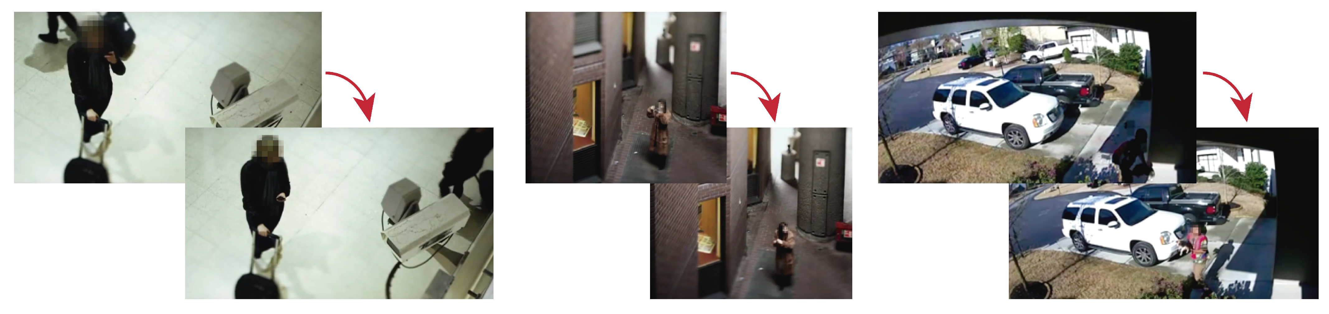
Defining what can be considered suspicious behavior is usually tricky, even for psychologists. In this work, the mentioned behavior is related to the commission of a crime, but it does not imply its realization (
Figure 1). For this research, we define suspicious behavior as a series of actions that happen before a crime occurs. In this context, our proposal focuses on shoplifting crime scenarios, particularly before the build-up phase situations that an average person may consider as typical conditions. Shoplifting crimes usually take place in supermarkets, malls, retail stores, and other similar businesses. Many of the models for addressing this problem need the suspect to commit a crime to detect it. Examples of such models include face detection of previous offenders [
5,
6] and object analysis in fitting rooms [
7]. In this work, we propose an approach to support the monitoring staff to focus on specific areas of screens where crime is more likely to happen. While existing models identify the crime itself, we model suspicious behavior as a way to anticipate a potential crime. In other words, we identify behaviors that usually take place before a shoplifting crime occurs. Then, the system can label a video: as containing suspicious or normal behavior. By detecting situations in a video that may indicate that suspicious behavior is present, the system indicates that a crime is likely to happen soon. The former gives the surveillance staff more opportunities to act, prevent, or even respond to such a crime. In the end, it is the security personnel who will decide how to proceed in each situation.
Overall, we propose a method to extract segments from videos that feed a model based on a 3D Convolutional Neural Network (3DCNN) for classifying behavior (as normal or suspicious). Once we train the model with such segments, it accurately classifies the behavior on a video dataset composed of daily action samples and shoplifting samples. Our results suggest that the proposed approach has applications in crime prevention in shoplifting cases.
As a summary, this work contributes to the literature mainly in three aspects.
It describes a methodology, the PCB method, to unify the processing and division of criminal video samples into useful segments that can later be used for feeding a Deep Learning (DL) model.
It represents the first implementation of a 3DCNN architecture to detect criminal intentions before an offender shows suspicious behavior.
It provides a set of experiments to validate the results, confirming that the proposed approach is suitable for such a challenging task: to detect criminal intention even before the suspect begins to behave suspiciously.
The remainder of this document is organized as follows. In
Section 2, we review various approaches that range from psychology to deep learning, to tackle behavior detection.
Section 3 presents the methodology followed to extract the relevant video segments used as input for our model, the PCB method, and the DL model architecture. The experiments, results, and their discussion are presented in
Section 4. Finally,
Section 5 presents the conclusions and future works derived from this investigation.
2. Background and Related Work
A surveillance environment must satisfy a particular set of requirements. Those requirements have promoted the creation of specialized tools, both on equipment and software, to support the surveillance task. The most common approaches include motion detection [
8,
9], face recognition [
5,
6,
10,
11], tracking [
12,
13,
14], loitering detection [
15], abandoned luggage detection [
16], crowd behavior [
17,
18,
19], and abnormal behavior [
20,
21]. Prevention and reaction are two primary aims in the surveillance context. Prevention requires forestalling and deterring crime execution. The monitoring staff must remain alert, watch as much as possible, and alert the ground personnel. Reaction, on the other hand, involves protocols and measures to respond to a specific event. The security teams take action only after the crime or event has taken place.
Most security support approaches focus on crime occurrence. Tsushita and Zin presented a snatching-detection algorithm, which performs background subtraction and pedestrian tracking to make a decision [
22]. Their approach divides the frame into eight areas and searches for a speed shift in one tracked person. Unfortunately, Tsushita and Zin’s algorithm can only alert when a person has already lost their belongings. Ullah et al. proposed a violence detection framework combining a trained MobileNet-SSD model [
23] for person detection and a C3D model [
24]. Besides, they optimize the trained model with the OPENVINO toolkit [
25]. They test their model with three different violence datasets: violent crowd [
26], violence in movies [
27], and hockey fight [
27]. Sultani et al. presented a real-world anomaly detection approach, training 13 anomalies, such as burglary, fighting, shooting, and vandalism [
28]. They use a 3DCNN for feature extraction and label the samples into two categories: normal and anomalous. Their model includes a ranking loss function and trains a fully connected neural network for decision-making. In a similar context, Nassarudin et al. [
29] presented a deep anomaly detection approach. They implemented a bilateral background subtraction, use the pretrained C3D model [
24] for feature extraction, and attached a fully connected network to perform regression. Using the UCF-Crime dataset [
30], they trained their model on 11 complete classes and tested their results on “robbery”, “fighting”, and “road accidents”. Ishikawa and Zin proposed a system to detect loitering people [
31]. Their system combines grid-based analysis, direction-based analysis, distance-based analysis, acceleration based analysis, and a decision-fusion stage of the people shown in the video to make a decision. Afra and Alhajj [
32] proposed a surveillance system that performs face detection and, according to the response, raises the alarm or tries to evaluate the suspect social media. Through security cameras, they collected images and processed them for face detection. They implemented the MobileNet-v1 [
23] architecture and trained on the WIDER face dataset [
33]. After the face location, they performed a face recognition by implementing two feature extraction techniques: OpenFace [
34] and Inception-Resnet-v1 [
35], trained on MS-Celeb-1M [
36].
Convolutional Neural Networks (CNN) have shown a remarkable performance in computer vision and other different areas in the last recent years. Particularly, 3DCNNs—an extension of CNN—focus on extracting spatial and temporal features from videos. Some interesting applications that have been implemented using 3DCNN include object recognition [
37], human action recognition [
38], gesture recognition [
39], and —particularly related to this work— behavior analysis from customers in the baking sector [
40]. Although all the works mentioned before involve using a 3DCNN, each one has a particular architecture and corresponding set of parameters to adjust. For example, concerning the number of layers, many approaches rely on simple structures that consist of two or three layers [
37,
38,
41], while others require several layers for exhaustive learning [
42,
43,
44,
45]. Recently, Alfaifi and Artoli [
46] proposed combining 3D CNN and LSTM for human action prediction (HAP). In their approach, the 3D CNN was used for feature extraction while the LSTM for classification. The model’s strength relies on the robustness to pose, illumination, and surrounding clutter. This robustness allows predicting human activity accurately. The architecture consists of a single 3D Conv layer, a 3D max-pooling layer, an long short-term memory (LSTM) layer, and two fully connected layers for classification.
Concerning shoplifting, the current literature is somewhat limited. Surveillance material is, in most cases, a company’s private property. The latter restricts the amount of data available for training and testing new surveillance models. For this reason, several approaches focus on training to detect normal behavior [
47,
48,
49,
50]. Anything that lies outside the cluster is considered abnormal. In general, surveillance videos contain only a small fraction of crime occurrences. Then, most of the videos in the data are likely to contain normal behavior. Many approaches have experienced problems regarding the limited availability of samples and their unbalanced category distribution. For this reason, some works have focused on developing models that learn with a minimal amount of data. As a reference, we include some representative works on the area of behavior detection in
Table 1.
Our work aims at developing a support approach for shoplifting crime prevention. Our model detects a person that, according to their behavior, is likely to commit a shoplifting crime. We achieve the latter by analyzing the people’s comportment in the videos before the crime occurs. To the best of our knowledge, this is the first work that analyzes behavior to anticipate a potential shoplifting crime.
3. Methodology
As part of this work, we propose a methodology to extract segments from videos where people exhibit behaviors relevant to shoplifting crime. The methodology considers both normal and suspicious behaviors, being the task to classify them accordingly. The following lines describe the dataset used and how we split it for experimental purposes, the pre-crime Behavior (PCB) method, and the 3DCNN architecture used for feature extraction and classification.
3.1. Description of The Dataset
Among the many works related to surveillance security, the analysis of non-verbal behavior is one of the less researched areas [
57]. This generates a lack of enhancement of security protocols and available information. Many works build their datasets using actors. However, they cannot catch the essential behavioral cues that an offender may show in a stressful situation. Some types of crimes have been more explored, such as crowd behavior, vandalism, fights, or assaults. For non-violent crimes, such as shoplifting, pickpocketing, or theft, it is harder to detect the crime in public places and get access to the videos.
In this work, we use the UCF-Crime dataset [
28] to analyze suspicious behavior during the build-up of a shoplifting crime. The dataset consists of 1900 real-world surveillance videos and provides around 129 h of videos. The videos have not been normalized in length and present a resolution of 320 × 240 pixels. The dataset includes scenarios from several people and locations, which are grouped into 13 classes such as “abuse”, “burglary”, and “explosion”, among others. We extracted the samples used in this investigation from the “shoplifting” and “normal” classes from the UCF-Crime dataset.
To feed our model, we require videos that show one or more people whose activities are visible before the crime is committed. Due to these restrictions, not all the videos in the dataset are useful. Suspicious behavior samples were extracted only from videos that exhibit a shoplifting crime, but to be used by our system, such samples must not contain the crime itself. Conversely, normal behavior samples were extracted from the “normal” class. Thus, it is important to stress that the model we propose is a behavior classifier (normal or suspicious) and not a crime classifier.
For processing the videos and extracting the suspicious behavior samples (video segments that exhibit suspicious behavior), we propose a novel method, the Pre-Crime Behavior (PCB) method, which we explain in the next section. Once we obtain the suspicious behavior samples, we applied some transformations to produce several smaller datasets. First, to reduce the computational resources required for training, all the frames were transformed into grayscale and resized to four resolutions: 160 × 120, 80 × 60, 40 × 30, and 32 × 24 pixels. As, by summing up normal and suspicious behavior samples, we get 120 samples, we applied a flipping procedure to increase such a number. Such a flipping procedure consists of turning over each frame of the video sample horizontally, resulting in a video where the actions happen in the opposite direction.
Data augmentation techniques aim to increase the number of useful examples in the training dataset, producing variations of the original images that the model is likely to see. Examples of these techniques include flipping, rotation, zoom, and brightness. It is relevant to mention that many of these techniques are not useful in our work. For example, vertical flipping an image makes no sense in our system as the videos will never be watched upside down. Rotation turns the image clockwise an arbitrary number of degrees, but it may drop pixels out of the image and produce areas with no pixels, which have to be filled in somehow. Zoom augmentation either adds new pixels around the image (zoom out) or leaves out part of the original image (zoom in), leading to losing or altering the scene’s information. The situations derived from using such data augmentation techniques could potentially do more harm than good and, for that reason, were not considered for this work. Given the reasons mentioned above, we considered that sticking only to horizontal flips was the most suitable strategy for this work. It generates additional training samples without adding or subtracting any information to the samples.
3.2. The Pre-Crime Behavior Method
Video sample segmentation does not follow a specific methodology in criminal intentions and suspicious behavior analysis. This makes it unreliable for creating a benchmark and testing a model across different video sets. For example, in some investigations, the segmentation is left to the experts’ judgement [
53,
55]. In others, the researchers select the frame before the criminal act [
54,
56]. In some particular cases, there is no segmentation at all [
22,
31,
51].
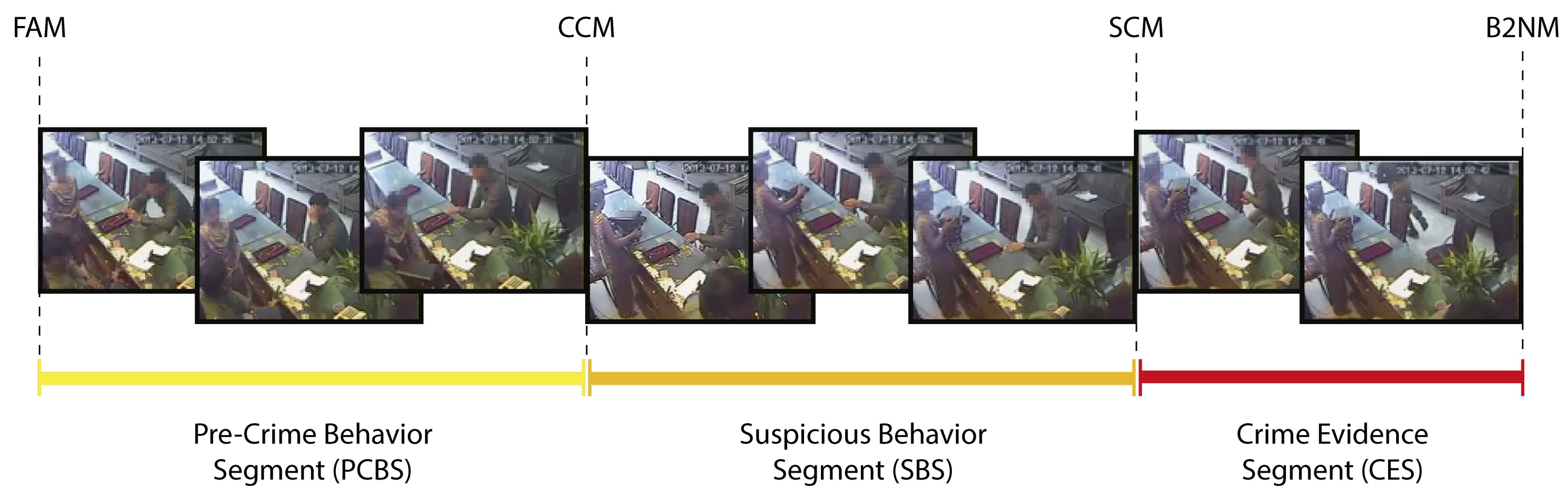
The Pre-Crime Behavior (PCB) method arises as a new proposal to unify moments, such as the build-up phase and the crime itself, and provide a new segment to the analysis, the suspect’s behavior before any aggression attempt. It is composed of four steps that allow the identification of four specific moments in the video sample. The PCB method is described as follows.
Identify the instant where the offender appears for the first time in the video. We refer to this moment as the First Appearance Moment (FAM). The analysis of suspicious behavior starts from this moment.
Detect the moment when the offender undoubtedly commits a crime. This moment is referred to as the Strict Crime Moment (SCM). This moment contains the necessary evidence to argue the crime commission.
Between the FAM and the SCM, find the moment where the offender starts acting suspiciously. The Comprehensive Crime Moment (CCM) starts as soon as we detect that the offender acts suspiciously in the video.
After the SCM, locate the moment where the crime ends (when everything seems to be ordinary again). If the video sample started from this instant, we would have no evidence of any crime committed in the past. This moment is known as the Back to Normality Moment (B2NM).
Please note that, as a sample video from the UCF-Crime dataset may contain more than one crime, the PCB method is applied once for each crime occurrence. Then, sometimes we can extract various suspicious behavior samples from the same video in the UCF-Crime dataset.
The output of the PCB method comprises four moments per crime in the input video. These four moments divide each sample into three relevant segments, as described below.
Pre-Crime Behavior Segment (PCBS). The PCBS is the video segment between the FAM and the CCM. This segment has the information needed to study how people behave before committing a crime, even acting suspiciously. Most human observers will fail to predict that a crime is about to occur by only watching the PCBS.
Suspicious Behavior Segment (SBS). The SBS is the video segment contained between the CCM and the SCM. The SBS provides specific information about an offender’s behavior before committing a crime.
Crime Evidence Segment (CES). The CES represents the video segment included between the SCM and the B2NM. This segment contains the evidence to accuse a person of committing a crime.
For the sake of clarity, we present the four moments and the three segments derived from the PCB method graphically, as depicted in
Figure 2.
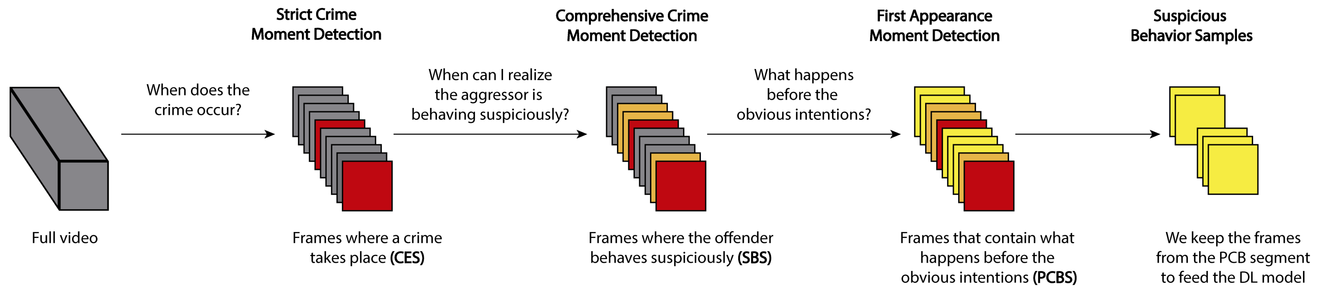
To extract the samples from the videos, we follow the process depicted in
Figure 3. Given a video that contains one or more shoplifting crimes, we identify the precise moment when the offense is committed. After that, we label the different suspicious moments—moments where a human observer doubts what a person in the video is doing. Finally, we select the segment before the suspect is preparing to commit the crime. These segments become the training samples for the Deep Learning (DL) model.
In a video sample, each segment has particular importance regarding the information it contains (see
Figure 2). The PCB segment has less information about the crime itself, but it allows us to analyze the suspect’s normal-acting behavior when they appears for the first time, even far from a potential crime. The SBS allows us to have a more precise idea about who may commit the crime, but it is not conclusive. Finally, the CES contains the doubtless evidence about a person committing a shoplifting crime. If we remove both the SBS and the CES from the video, the result will be a video containing only people shopping, and there will be no suspicion or evidence that someone commits a crime. That is the importance of the accurate segmentation of the video. From the end of a CES until the next SBS, there is new evidence about how a person behaves before attempting a shoplifting crime.
For experimental purposes, we only use the frames from the PCBS in this work. As these segments lack specific criminal behavior, they have no information about any transgression. The PCB segments are ideal for feeding our 3DCNN model, aiming to characterize the people’s behavior. The objective of the model is to identify when such behavior is suspicious, which may indicate that a shoplifting crime is about to be committed.
3.3. 3D Convolutional Neural Networks
For this work, we use a 3DCNN for feature extraction and classification. 3DCNN is a recent approach for spatio-temporal analysis that has shown remarkable performance in processing videos in different areas, such as moving objects action recognition [
37], gesture recognition [
39], and action recognition [
38]. We decided to implement a 3DCNN in a more challenging context, such as searching for patterns in video samples, which lack suspicious and illegal visual behavior.
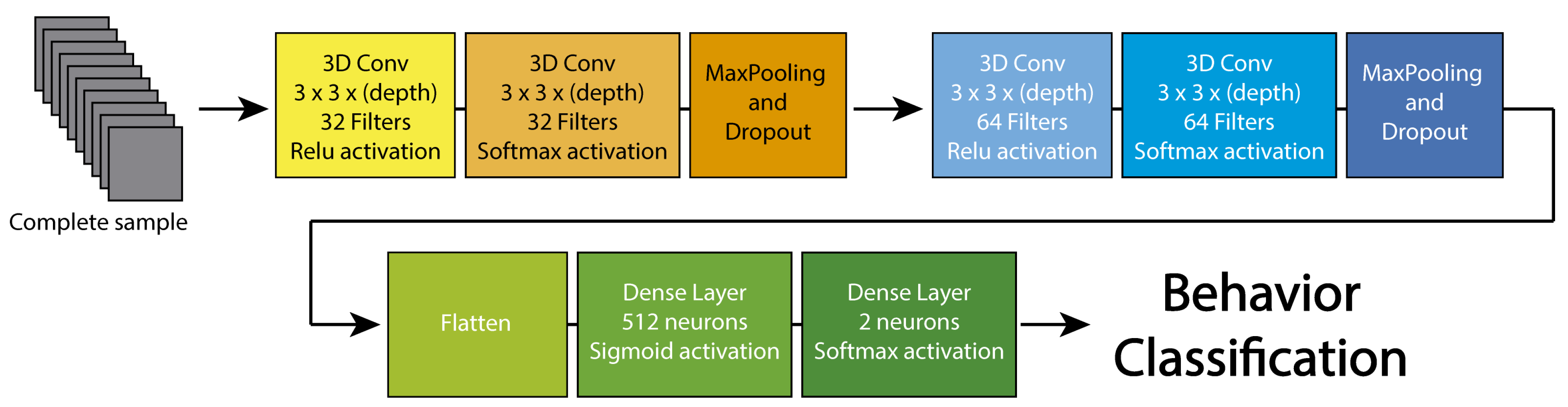
We employ a basic structure to explore the performance of the 3DCNN for behavior classification. The model comprises four Conv3D layers (two pairs of consecutive convolutional layers for capturing long dependencies [
43,
58,
59]), two max-pooling layers, and two fully connected layers. As a default configuration, in the first pair of Conv3D layers, we apply 32 filters, and for the second pair, 64 filters. All kernels have a size of 3 × 3 × 3, and the model uses an Adam optimizer and cross-entropy for loss calculation. The graphical representation of this model is shown in
Figure 4. The last part of the model contains two dense layers with 512 and two neurons, respectively. This architecture was selected because it has been used for similar applications [
60], and it seems suitable as a first approach for behavior detection in surveillance videos.
For handling the model training, we use Google Colaboratory [
61]. This free cloud tool allows us to write and execute code in cells and runs directly on a browser to train DL models. We can upload the datasets to a storage service, link the files, prepare the training environment, and save considerable time during the model training using a virtual GPU.
3.4. Metrics
As the decisive metric to analyze the results, we considered the accuracy (Equation (
1)). It considers the correct hits—true positive (TP) plus true negative (TN)—over the total number of samples evaluated (
and
represent false positives and false negatives, respectively).
As accuracy shows the general performance of the model, we complement its information by presenting the confusion matrices of the best runs. These matrices allow checking, in detail, the model capability to classify suspicious and normal behavior. We used two additional metrics for adequately analyzing the results from the confusion matrices: precision (Equation (
2)) and recall (Equation (
3)). Precision indicates the proportion of samples classified as suspicious that are, in fact, suspicious—a model with a precision of 1.0 produces no
. Recall indicates the proportion of actual suspicious samples that were correctly classified by the system—a model with a recall of 1.0 produces no
.
4. Experiments And Results
We conducted a total of six experiments in this work. These experiments are divided into two categories: preliminary and confirmatory. The first four experiments are preliminary as they focus on exploring the effect of different configurations under different scenarios, aiming to find some suitable configurations that may lead to better model performance. We refer to the last two experiments as confirmatory as we tested the system on more challenging configurations derived from the preliminary experiments, to validate the approach. Among all these experiments, a total of 708 models were generated and tested. Although the specific details of each experiment are detailed in its corresponding description, for the ease of the reader, we have provided an overview of our experimental setup in
Figure 5.
4.1. Preliminary Experiments
In this set of experiments, we explore different configurations for the system and estimate their effect on its overall performance in terms of the accuracy obtained. The rationale behind this first set of experiments is that we affect the model’s performance by introducing small variations on its parameters. Then, finding a good set of input parameters is a way to improve the overall performance of the model.
For this work, four parameters have been considered for tuning purposes. These parameters, as well as their available values, are listed below.
Training set size. The percentage of the samples from the base dataset used for training. The possible values are 80%, 70%, and 60%. Note that, as an attempt to test out approach on different situations, the base dataset changes for each particular experiment.
Depth. The number of consecutive frames used for 3D convolution. The values allowed for this parameter are 10, 30, and 90 frames.
Resolution. The size of the input images (in pixels). We used four different values for resolution: 32 × 24, 40 × 30, 80 × 60, and 160 × 120 pixels.
Flip. As discussed before, to increase the number of samples, we applied a horizontal flipping procedure to all the samples. By using this procedure, we doubled the number of samples. Stating that a set has been flipped indicates that the frames in those videos have been flipped horizontally.
To evaluate the impact of varying the values for these parameters, we conducted five independent experiments. Each of these experiments followed a factorial design with two factors (one factor per parameter). In all the experiments, one of the factors was always the resolution in pixels. We trained three independent models per combination of such factors. The results are analyzed both from the statistical perspective (main effects and interaction effects through a two-way ANOVA) and the practical one (by analyzing the interaction plots and the average accuracy derived from the observations). It is relevant to mention that all the cases satisfied both normality and homogeneity of the variances, which are conditions required to apply the two-way ANOVA. We tested normality by analyzing the residuals and through the Shapiro–Wilk test of normality, while we applied the Levene’s test to check the homogeneity of variances within groups. The significance value considered for all the statistical tests in this work was 5%.
4.1.1. Experiment P01—Effect of the Depth (In Balanced Datasets)
To analyze the impact of varying the depth size (number of consecutive frames to consider) under different resolutions, we analyzed its effect on a balanced dataset containing 30 normal behavior samples and 30 suspicious behavior ones, where 80% of those samples were used for training the models. As there were, as explained before, three values allowed for the depth: 10, 30, and 90 frames, and four values for the resolution: 32 × 24, 40 × 30, 80 × 60, and 160 × 120 pixels, the combinations of these parameters resulted in 12 configurations. For each configuration, we conducted three independent runs to generate three models. With this data, we ran a two-way ANOVA to analyze the effect of depth and resolution on the accuracy of the model, given the base configuration.
Table 2 presents the accuracy of the three independent models trained for each configuration and their average accuracy per configuration.
By analyzing the statistical results, we found that neither the main effects are significant, nor their interaction (with a significance level of 5%). The
p-values obtained from the two-way ANOVA for the main effects of depth and resolution in this experiment were 0.1044 and 0.6488, respectively. The
p-value for their interaction was 0.9502. As there is no statistical evidence that suggests that changes in the depth or the resolution affect the accuracy of the model, we extended the analysis and considered inspecting the interaction plot, which is depicted in
Figure 6. This interaction plot suggests that independently of the depth considered, using 160 × 120 pixels as resolution obtains the worst results. Furthermore, based only on the 36 observations analyzed, using ten frames and 32 × 24 pixels obtains the best average results on the fixed values used for this experiment. For this reason—and based on the fact that we could not derive any other conclusion from the statistical perspective—we considered using ten frames as the best value for depth for the next set of experiments.
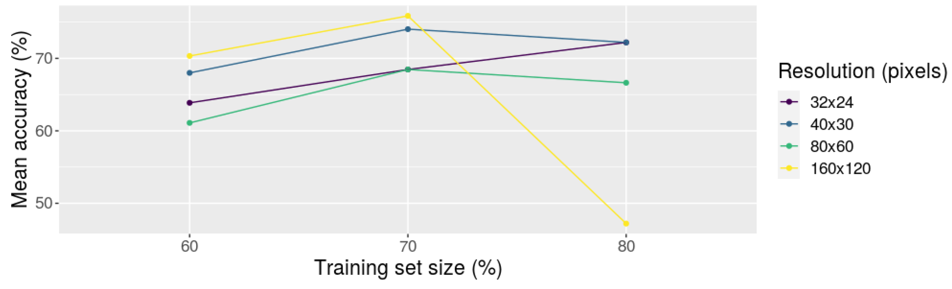
4.1.2. Experiment P02—Effect of the Training Set Size (In Balanced Datasets)
In this experiment, we changed the proportion of samples used for training, combined with four values of the resolution, as an attempt to estimate their effect on the model’s accuracy. As in the previous experiment, the dataset is also balanced with 30 normal behavior samples and 30 suspicious behavior ones. However, for this experiment, the depth parameter was fixed to 10. This value was taken from the previous experiment since we obtained the best results by using ten frames. We allowed three values for defining the training set size: 80%, 70%, and 60% of the total of samples in the dataset (that contains 60 samples as previously described). As in the previous experiment, the available values for the resolution were 32 × 24, 40 × 30, 80 × 60, and 160 × 120 pixels. For each configuration, we trained three independent models and used their accuracy to run a two-way ANOVA to analyze both the main and interaction effects of the two variables, given the base sample set. The accuracy of the three independent models per configuration is shown in
Table 3.
The statistical analysis through a two-way ANOVA showed that the main effects, the proportion of samples used for training and the resolution, are not significant with (the p-values were 0.0140 and 0.0771, respectively). However, their interaction was statistically significant, with a p-value of 0.0004. Because the interaction effect was statistically significant, we compared all group means from the interaction of the two factors. The p-values were adjusted by using the Tukey method for comparing a family of 12 configurations. The results suggested that the worst combination arose when using 80% of the base dataset for training and 160 × 120 pixels as resolution. The confidence interval for the average accuracy (with 95% of confidence), lies between 36.6% and 57.8%. Conversely, the remaining configurations are considered equally useful from the statistical perspective, since their confidence intervals overlap.
To have a better look at the behavior of these configurations, we also analyzed the interaction plot of the proportion of samples from the base dataset used for training and the resolution (
Figure 7). The interaction plot confirmed the idea that using 80% and 160 × 120 pixels harms the process. So far, we do not have an explanation for such behavior yet. However, we can also observe how similar the remaining configurations are, in terms of accuracy. As the best results in this experiment were obtained by using 70% of the base dataset for training purposes, we kept this value as a recommended one for the following experiments.
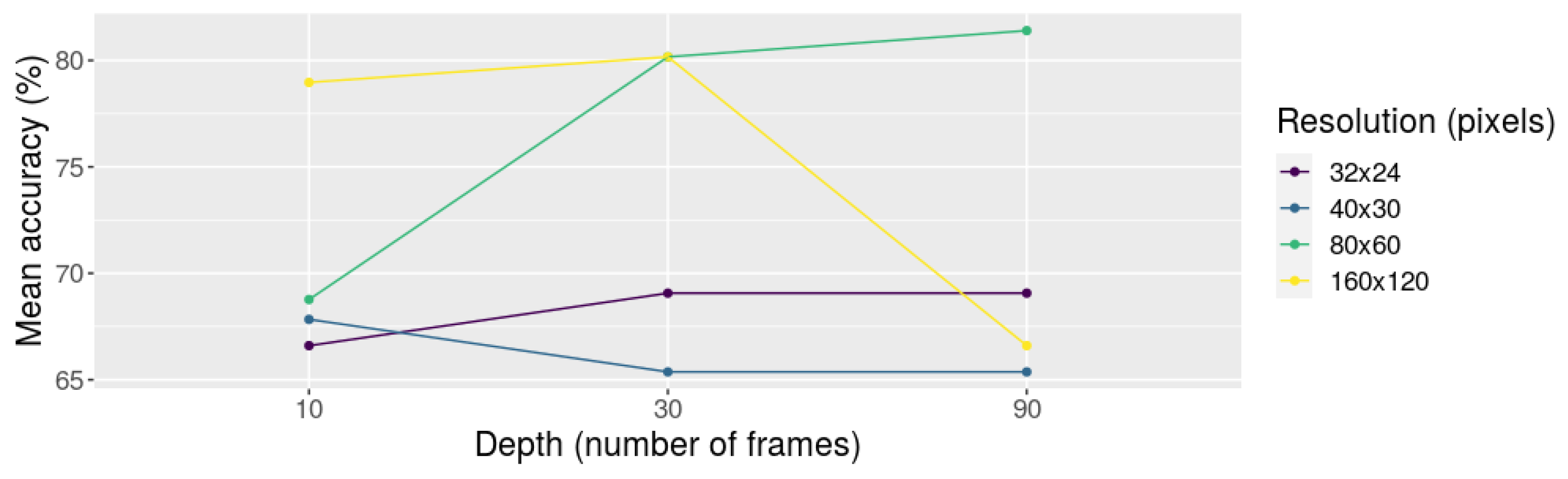
4.1.3. Experiment P03—Effect of the Depth (In Unbalanced Datasets)
At this point, we had only explored the behavior of the models in balanced sets (same proportion of normal behavior and suspicious behavior samples). For this experiment, we analyzed the effect of the depth and the resolution (as we did in experiment P01), but this time on an unbalanced set that contains 90 samples (60 normal behavior samples and 30 suspicious behavior ones). As we learned from the previous experiment, the models obtained the best performance when 70% of the base dataset was used for training. Then, we used such a value for this experiment. For the depth, three values were allowed: 10, 30, and 90 frames, while four values were available for the resolution: 32 × 24, 40 × 30, 80 × 60, and 160 × 120 pixels. The combinations of these parameters give 12 configurations. For each of these configurations, we trained three independent models. The results from this experiment, in terms of accuracy, are depicted in
Table 4.
The statistical analysis through the two-way ANOVA suggests that the effect of the depth is not statistically significant (p-value of 0.1786). However, the effect of the resolution, as well as the interaction between the depth and the resolution, are statistically significant with p-values of 7.09 and 0.0031, respectively. As the interaction between the depth and the resolution is important in this case, we used the Tukey method for comparing a set of 12 configurations and adjusting the p-values, as we did in the previous experiment. The results show that the configurations can be classified into four groups, based on the accuracy obtained. However, these groups overlap for many of the configurations. Based on the confidence intervals for the average accuracy of the models (with 95% of confidence), the configuration with the most promising confidence interval for the average accuracy was using 90 frames and 80 × 60 pixels as resolution.
For clarity, we also included the interaction plot as we did for the previous experiments.
Figure 8 suggests that, in unbalanced sets, the combination of depth and resolution is important to get a good accuracy. The information from the interaction plot seems to indicate that, for large resolutions such as 160 × 120 pixels, increasing the number of frames decreases the model’s accuracy. Conversely, for slightly lower resolutions such as 80 × 60 pixels, increasing the number of frames improves the model’s accuracy. Then, based on the statistical results as well as the analysis of the interaction plot, we can recommend that, when dealing with unbalanced sets, the best configuration is to use 90 frames and 80 × 60 pixels.
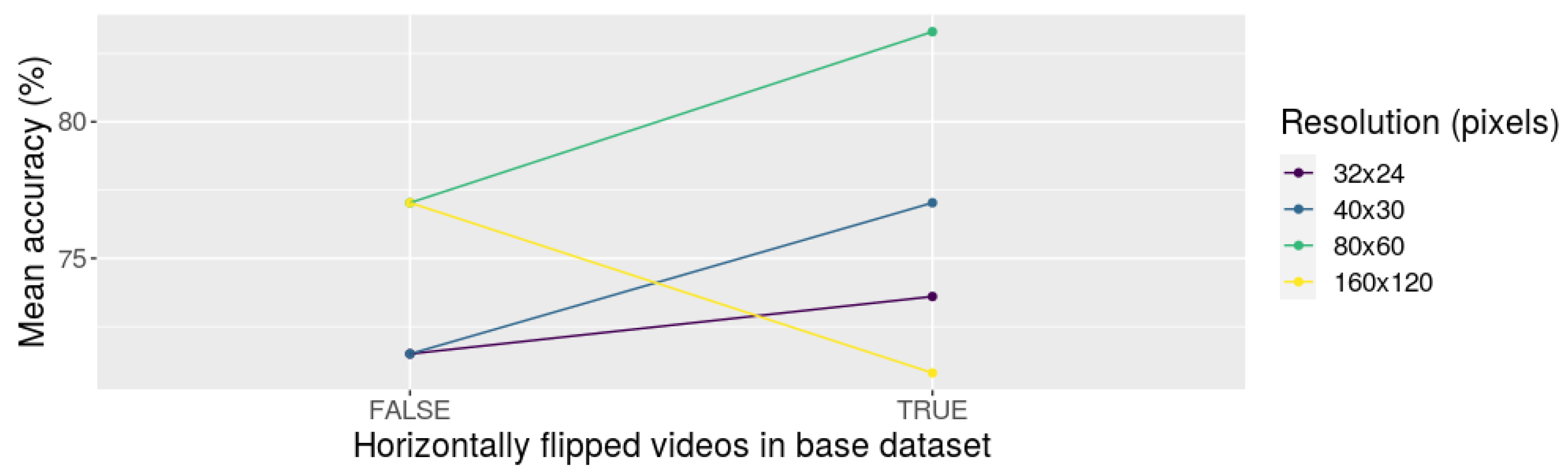
4.1.4. Experiment P04—Effect of the Data Augmentation Technique (In Balanced Datasets)
Data augmentation techniques are an option to take advantage of small datasets. For this reason, we tested the model performance using original and horizontally flipped images in different runs. The training set has a size of 60% (
Table 5 and
Figure 9) and 70% (
Table 6 and
Figure 10) of the total dataset.
When 60% of the dataset was used for training, we found that the effect of using data augmentation is not significant (its
p-value was 0.1736). However, the effect of the resolution is significant, given a
p-value of 0.0050. The
p-value for the interaction of these two factors was 0.0176, which is significant, with a 5% of significance. To extend the analysis, we also provide the interaction plot of these two factors, which is depicted in
Figure 9. As it can be observed, including the horizontally flipped samples, in general, increases the model’s performance. The only configuration that seems to contradict this trend is when the resolution is set to 160 × 120 pixels. We do not have a concrete explanation of this behavior, but it could be related to the computing power related to learning at a higher resolution.
When 70% of the dataset was used for training, we could not found evidence that the main effects, and neither their interaction, were significant. However, the effect of the resolution is significant with
(the
p-values were 0.0.1797, 0.1051, and 0.2248, respectively). To deepen this situation, we present the interaction plot of these two factors, which is depicted in
Figure 10. Based on the interaction plot, using 70% of the dataset when horizontally flipped samples are included does not affect the model’s performance. The only configuration that seems to contradict this idea is when the resolution is set to 80 × 60 pixels. In this case, we cannot explain why this situation occurred. Further research in this regard will be needed to explain this behavior.
As the experiments with 60% and 70% obtained similar results in terms of accuracy, we considered that any of these configurations could effectively be used to train the model. Then, we kept 70% as the proportion of samples to be used for training in the remaining experiments.
4.2. Confirmatory Experiments
For the confirmatory experiments, we focused on analyzing our model on larger datasets that include horizontally flipped samples. For this purpose, we analyzed the effect of the depth and resolution (as we did in experiment P01) but this time on larger sets that included horizontally flipped samples. The first dataset contains 240 samples (120 normal behavior samples and 120 suspicious behavior ones) while the second contains 180 samples (120 normal behavior samples and only 60 suspicious behavior ones). However, these samples are not independent as they include flipped ones. When we refer to the number of samples, we mean the number of available videos, regardless of being the original ones extracted using the PCB method or their flipped versions. Based on the proportion of normal and suspicious samples in each dataset, we can state that the first one is “balanced”, while the second one is not. As we learned from the previous experiment, the training set corresponds to 70% of the base dataset.
4.2.1. Experiment C01—Effect of the Depth (In Larger Balanced and Unbalanced Datasets with Data Augmentation)
First, for the depth, three values were allowed: 10, 30, and 90 frames, while four values were available for the resolution: 32 × 24, 40 × 30, 80 × 60, and 160 × 120 pixels. Then, for each set, the combinations of depth and resolution produce 12 different configurations. The results of this experiment are depicted in
Table 7 and
Table 8.
In the case of the balanced dataset (
Table 7), the best average results are mainly obtained when 30 frames are used. If we consider the resolution, it seems that 80 × 60 is the best choice. In general, it seems that using 90 frames affects the model’s performance. The results are similar when the unbalanced dataset is used (
Table 8). However, this time there is one case where using 90 frames produced the best average results (when combined with 40 × 30 pixels as resolution).
4.2.2. Experiment C02—Aiming for the Best Model
Based on the results from the previous experiment, we analyzed the results to decide which parameters might improve behavior classification, and selected the configurations with the best performance. Then, the depth of 90 frames was excluded from this experiment. We repeated the configurations used in the previous experiment (excluding the 90 frames as depth), but this time running 30 times each configuration. Besides, this time we used using cross-validation, to extend the results previously obtained.
Table 9 presents average accuracy and the standard deviation of each configuration tested in experiment C02. Most of the results have an accuracy of around 70%. As observed, there is no significant deviation in each training group. The results seem very similar among them. However, the results when 10 frames and 80 × 60 pixels are used is slightly better than the rest. On an individual level, the best model was also obtained when this resolution was used. The best model correctly classified 92.50% of the samples.
On a final test, we used the best model obtained to solve the four configurations available when 80 × 60 pixels are used. This way, we tested the model on the balanced dataset with 10 and 30 frames, and in the unbalanced dataset, also with 10 and 30 frames. The results are presented in terms of the confusion matrices, as shown in
Figure 11. To deepen the results, we present the precision and recall for each class in isolation. For suspicious behavior, the model presents a precision that ranges from 0.7826 (unbalanced dataset with 30 frames) to 0.8571 (balanced dataset with 10 frames). This means that when the model classifies a behavior as suspicious, it is correct in at least 78% of the cases. Regarding the recall for suspicious behavior, it is equal to 1 in all cases. This means that the model correctly classifies all the suspicious behavior samples in the test set (no suspicious sample was classified as a normal one). For normal behavior, the model’s precision is always equal to 1, meaning that whenever the model predicts that a sample is normal, the model is always correct. Regarding the recall for normal behavior, the values range from 0.8055 (balanced dataset with 30 frames) to 0.8888 (unbalanced dataset with 10 frames), which means that the best model correctly classifies 88% of the normal behavior samples in the unbalanced dataset with 10 frames of depth.
4.3. Discussion
There are some aspects related to the proposed model and the results obtained so far that are worth discussing:
The system can be used to classify normal and suspicious behavior given the proper conditions.
The PCB method exhibits some limitations as it is yet a manual process.
The time needed for training the models suggests that training time may not be related to accuracy.
There is an apparent relationship between the model’s performance and the number of parameters in the models.
The following lines deepen into these critical aspects.
As the first experiment in this work, we selected a 3D Convolutional Neural Network with a basic configuration as a base model. Then, we tried different configurations as a means for parameter tuning. The result of this process was a configuration that improved the performance of the model. From the parameter exploration phase, we found that 80 × 60 and 160 × 120 resolutions delivered better results than a commonly used low resolution. This experiment was limited to a maximum resolution of 160 × 120 due to processing resources. Another significant aspect to consider is the “depth” parameter. This parameter describes the number of consecutive frames used to perform the 3D convolution. After testing different values, we observed that small values, between 10 and 30 frames, show a good trade-off between image detail and processing time. These two factors impact the network model training and the correct classification of the samples. Furthermore, the proposed model can correctly handle flipped images and unbalanced datasets. We confirmed this idea through the experiments performed on a more realistic simulation where the dataset has more normal behavior samples than suspicious behavior ones.
It is important to clarify the process for extracting the behavior samples from the UCF-Crime dataset. We are aware of the problems that may arise from using a non-automated method to extract the video segments from the original dataset. For example, (1) as it is a manual process, it is restricted to small datasets, and (2) due to its subjectivity, different executions may lead to different video segments (even if the same observer is involved). Although the PCB method exhibits those limitations, no other investigation has addressed this problem in the way we propose. Then, the PCB method is the only systematic technique we have to extract behavioral information in the way we need it, from the original dataset. For the sake of reproducibility, we have included a relation of the segments of videos from the UCF-Crime dataset that we used as input for the DL models in this work. This information can be consulted in the appendices, in
Table A1 and
Table A2. Then, any future work that wants to use our video samples can use such segments—without the need to rerun the PCB method.
Regarding the processing time, we use Google Colaboratory to perform the experiments in this work. This tool is based on Jupyter Notebooks and allows using the GPU. The speed of each training depends on the tool demand. Most of the networks in this investigation were trained in less than an hour. However, a higher GPU demand may impact the training time. At the moment, we cannot establish a formal relationship between the resolutions of the videos and the training time, but we have an estimation of how different depths impacted the training time.
Table 10 shows the average training times of models generated for experiment C01, as described in
Section 4.2.1 (the results of these experiments are shown in
Table 7 and
Table 8). From these results, it is clear that using a higher resolution and a larger depth increases the computational resources required for the training. In our particular case, some of the runs on the higher resolution (160 × 120) and maximum number of frames (90) took up to four hours. This information should be taken into consideration for further studies as the training time is an essential factor and, in this case, we are dealing with datasets that can be considered small. Besides, another point to consider is the model’s accuracy against the training time required to generate such a model. Although the training time drastically increases when the resolution increases, the accuracy does not increase in a similar proportion. Particularly, we found cases where increasing the resolution worsen the accuracy of the models produced.
As the results from the confirmatory experiments suggest, the 80 × 60 input resolution generates the best accuracy values. Although we have not confirmed our ideas, we think the accuracy might be related to the network’s number of parameters and image information. A balance between these two parameters may impact the final result. While smaller resolutions mean fewer parameters, it also means less information to model the offender’s behavior. On the contrary, a big resolution could give more details in visual data to analyze, but also imply more processing and many more parameters to optimize. Thus, we think this balance between resolution and parameters might cause an improvement in the model’s accuracy. However, more research is required to support this claim.
5. Conclusions
For this work, we have focused on the behavior performed by a person during the build-up phase of a shoplifting crime. The neural network model identifies the previous conduct, looking for suspicious behavior, and not recognizing the crime itself. This behavior analysis is the principal reason why we remove the committed crime segment from the video samples, to allow the artificial model to focus on decisive conduct and not in the offense. We implement a 3D Convolutional Neural Network due to its capability to obtain abstract features from signals and images, based on previous action recognition and movement detection approaches.
Based on the results obtained from the conducted experimentation, 75% of accuracy in suspicious behavior detection. Then, we can state that it is possible to model a person’s suspicious behavior in the shoplifting context. We found which parameters fit better for behavior analysis through the presented experimentation, particularly for the shoplifting context. We explore different parameters and configurations, and, in the end, we compare our results against a reference 3D Convolutional architecture. The proposed model demonstrates a better performance with balanced and unbalanced datasets using the particular configuration obtained from previous experiments.
The final intention of this experimentation is to develop a tool capable of supporting the surveillance staff, presenting visual behavioral cues, and this work is a first step to achieve the mentioned goal. We will explore different aspects that will contribute to the project development, such as bigger datasets, adding more criminal contexts that present suspicious behavior, and real-time tests.
In these experiments, we used a selected number of videos from the UCF-Crimes dataset. As future work, and aiming at testing our model in a more realistic simulation, we will increase the number of samples, preferably the normal behavior ones, to create a bigger sample imbalance between classes. Another exciting aspect of the development of this project is expanding our behavior detection model to other contexts. It exists many situations where we can find suspicious behavior, such as stealing, arson intents, and burglary. We will gather videos of different contexts to strengthen the capability to detect suspicious behavior. Finally, the automation of the PCB method for video segmentation stands out as an interesting point to explore. This will reduce the preprocessing time, which would allow analyzing a larger amount of data. For this reason, we consider this an important path for future work derived from this investigation.

 ,
, 


