Dam Breach Simulation with the Material Point Method

Department of Computer Science, Kansas State University, Manhattan, KS 66506, USA
*
Author to whom correspondence should be addressed.
†
Current address: Department of Computer Science, 2184 Engineering Hall, Manhattan, KS 66506, USA.
‡
These authors contributed equally to this work.
Computation 2021, 9(2), 8; https://0-doi-org.brum.beds.ac.uk/10.3390/computation9020008
Submission received: 16 December 2020
/
Revised: 13 January 2021
/
Accepted: 18 January 2021
/
Published: 20 January 2021
(This article belongs to the Section Computational Engineering)
Abstract
:Dam embankment breaches caused by overtopping or internal erosion can impact both life and property downstream. It is important to accurately predict the amount of erosion, peak discharge, and the resulting downstream flow. This paper presents a new model based on the material point method to simulate soil and water interaction and predict failure rate parameters. The model assumes that the dam consists of a homogeneous embankment constructed with cohesive soil, and water inflow is defined by a hydrograph using other readily available reach routing software. The model uses continuum mixture theory to describe each phase where each species individually obeys the conservation of mass and momentum. A two-grid material point method is used to discretize the governing equations. The Drucker–Prager plastic flow model, combined with a Hencky strain-based hyperelasticity model, is used to compute soil stress. Water is modeled as a weakly compressible fluid. Analysis of the model demonstrates the efficacy of our approach for existing examples of overtopping dam breach, dam failures, and collisions. Simulation results from our model are compared with a physical-based breach model, WinDAM C. The new model can capture water and soil interaction at a finer granularity than WinDAM C. The new model gradually removes the granular material during the breach process. The impact of material properties on the dam breach process is also analyzed.
1. Introduction
Most flood routing of water through water control structures (dams) before the middle 1960s was computed manually. Then, routing software on computers began to replace manual methods. In the 1990s, approximately one hundred sites were selected for more in-depth evaluation, data collection, and data analysis. Additional tests were conducted in the USDA-ARS outdoor Hydraulic Engineering Research Unit (HERU) Laboratory near Stillwater, Oklahoma. Kansas State University cooperated with the USDA to develop software for water control structure design and simulation analysis. Advances in scientific computing capability have enabled more advanced tools to be developed to benefit all types of hydraulic science research.
Interest in the potential flooding due to overtopping has existed for years. There are many simulation processes that can be accurately modeled using computer simulation. Fluid simulation methods are divided into Eulerian and Lagrangian methods. The most popular fluid simulation approach using the Eulerian method is Computational Fluid Dynamics (CFD). CFD for dam break simulation has been extensively investigated [1,2,3]. CFD supports three discretization methods: finite difference, finite volume, and finite element methods. These three discretization methods use distinct mathematical models and governing equations for computation. In our previous study [4,5], we explored the Finite Volume Method(FVM) for dam breach simulation using the open-source toolbox OpenFOAM. Cao and Neilsen [5] simulated the flooding due to overtopping without considering the deformation of the solid dam structure.
Unlike Eulerian methods, there is no numerical dispersion term in the Lagrangian method. Therefore, Lagrangian techniques are useful for simulations when large topological changes occur in the fluid interface. Smoothed Particle Hydrodynamics (SPH) is a well-known method in the computer simulation field. Instead of considering the dam embankment structure as a solid body material as in [4,5], the granular material, like soil, can be represented as either a continuum or a set of individual particles using SPH. SPH is used to simulate large surface flows [6,7] and dam break flows [8,9,10].
In addition, the Discrete Element Method (DEM) is a very popular particle-based system to handle fluid simulation. Often, CFD is coupled with the DEM in many studies and engineering fields including rock slides [11,12], granular flow in water reservoirs [13,14], fluid-particle interaction in dam breaks [15,16]. Other than the CFD-DEM, the coupled SPH-DEM is encountered in many multi-species simulation studies as well. Rungjiratananon et al. simulated sand-water interaction in real time using a hybrid SPH-DEM [17]. Wu et al. [18] and Canelas [19] used the SPH-DEM to simulate multi-phase free surface flow. Lenaerts and Dutré [20] also proposed a dynamics framework for the simulation of both fluid and porous granular material using SPH-DEM.
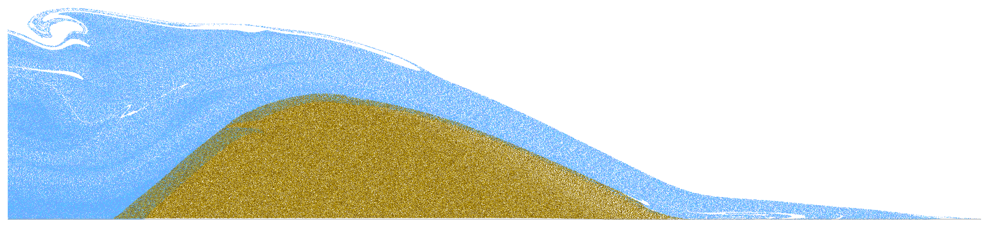
Another approach, the Material Point Method (MPM), was initially introduced by Sulsky [21] and used to tackle more complex problems. The MPM computes forces using a fixed Eulerian grid, while it also stores information on Lagrangian particles. The fixed grid handles the topology changes like collisions between the material. The MPM stores the information using two distinct representations, and it must be transferred between them. The MPM also avoids re-meshing and storing connectivity between particles. The large deformation landslide problem using the MPM has been widely investigated. Soga et al. [22] introduced MPM to analyze large deformation of landslide mass movements and post-failure behavior. Troncone et al. [23,24] used the MPM to simulate landslide triggered by an increase in the groundwater level or water pressure. Yerro et al. [25,26] applied the MPM to analyze landslides for brittle soils or unsaturated soils. Furthermore, there is much potentiality of the MPM for analyzing geotechnical problems including the landslide that occurred at Oso in USA [27], the landslides of Senise and Maierato in Italy [28,29], and the Sainte-Monique landslide [30]. Dong et al. applied the MPM to solve submarine landslide problems [31,32]. In this paper, we use MPM for overtopping dam breach simulation as shown in Figure 1.
To handle multi-species interactions such as water and porous soil [33], Bandara et al. [34,35] introduced models for soil deformation and porous fluid flow using the MPM. Tampubolon et al. [36] simulated the interaction of sand and water mixtures using the MPM and obtained encouraging results. For the porous material property, Klár et al. [37] used the improved Drucker–Prager plastic flow model with volume correction. For the MPM implementation, Arduino et al. [38] and Jassim et al. [39] examined that momentum exchange using the two-grid MPM for the multi-species interaction.
For dam safety simulation, the two most common approaches for the discretization of solids or liquids are Eulerian or Lagrangian. For Eulerian-based methods, the quantities of interest are in fixed locations or fixed grids such as in CFD or CFD-DEM mesh modeling. For the Lagrangian-based methods, the quantities of interest are attached to the materials including the SPH, SPH-DEM, and MPM particle-based methods. Among these modeling methods, in order to simulate dam erosion with multi-species interactions between soil and water, the proposed new dam simulation models use the material point method, which combines the aspects of both types of discretization.
In particular, we construct a new model for the multi-species material point method to allow interaction between soil and water. We allow wet soil transitions from cohesive grains to flowing sediment as water saturation increases. We create an overtopping dam erosion simulation model using multi-species particles and a two-grid material point method. For validation, the MPM simulation model of overtopping dam erosion is compared with available experimental data and the results of other physical-based models like WinDAM [40].
2. Mathematical Background
Tampubolon and Angeles [36], Atktn and Craine [41], and Borja [42] all considered multi-species using mixture theory. Therefore, the soil and water were modeled as a multi-species continuum using mixture theory.
2.1. Conservation Laws
The conservation of mass and the conservation of momentum are calculated individually, and each species obeys the following conservation laws with respect to its own motion. Conservation of mass, represented by the following equation, means that the quantity of mass in the system remains constant over time.
Likewise, conservation of linear momentum is represented by the following equation.
Here, the superscript s is used to represent soil, w is used to represent water, total mass density is , and total momentum is the sum . The velocity . After summing the two species, the standard conservation of mass is obtained in (1), and we also note that the conservation of linear momentum for the individual species implies the conservation of linear momentum for the mixture (2).
2.2. Deformation Gradient
The deformation gradient represents how deformed the material is locally. It is used to measure how the material has locally rotated and deformed due to its motion [36]. Plasticity is represented by factoring the deformation gradient into elastic and plastic parts as [37].
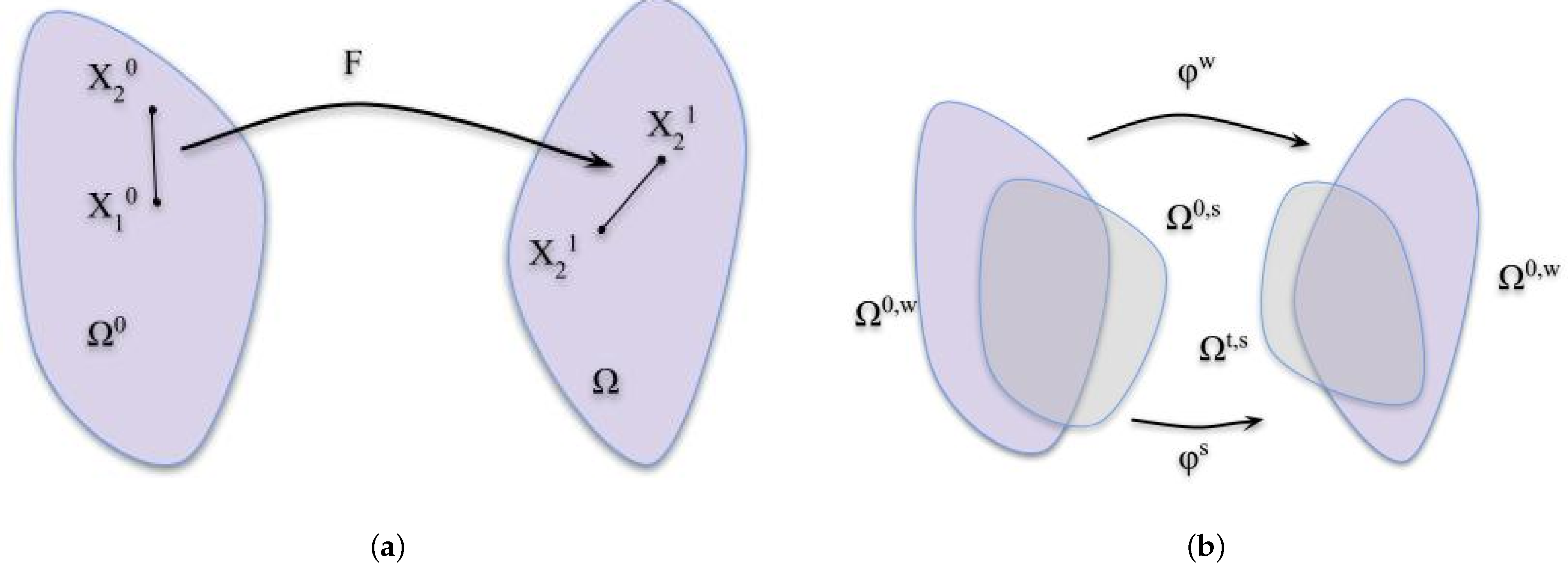
By factoring the deformation gradient in this way, the deformation history is divided into two pieces, plastic deformation and elastic deformation . Figure 2a shows the single-phase deformation gradient F and the material properties. Figure 2b displays the material property for multi-phase deformation between water and soil, and the overlapping region is captured through momentum exchange.
2.3. Constitutive Model
2.3.1. Soil Model
Tampubolon and Angeles [36] modified the model of Klár et al. [37] to include cohesive stresses for a porous material and water mixture. Therefore, the amount of cohesion varies with the saturation of water in the mixture. The soil partial stress is defined in terms of the hyper-elastic potential energy density as:
is the deformation gradient of soil motion. The and terms arise because of the potential energy density in terms of the deformation gradient. As done in finite strain elastoplasticity [43], defines plastic flow for porous soil. represents the compression and shearing, while represents the sliding and separation. The Drucker–Prager [44] plastic flow and yield condition is used to determine the elastic and plastic deformation gradient. The Drucker–Prager yield criterion is a pressure-dependent model, and the criterion was introduced to deal with the plastic deformation of soils. Bonet and Wood [43] provided the background for elastoplastic constitutive modeling. Dry porous material can be modeled effectively with the assumption made by Drucker–Prager since the yield condition is defined by the constraint that shear stress should be no larger than the compressive normal stress in all directions [36]. For the elastic part of the constitutive behavior for the soil phase, the elastic potential energy density is defined in terms of the logarithmic strain as:
Cohesive effects can be modeled by modifying the elastic stress yield condition to be:
where is the singular decomposition of and , is the spatial dimension, and increases with the amount of cohesion in the material.
2.3.2. Water Model
Water is modeled as incompressible [45] with partial stress:
is the water pressure. is the ratio of the current to initial local volume of material in the water phase.
where is the bulk modulus of the water and is a term that more stiffly penalizes large deviations from incompressibility.
2.3.3. Momentum Exchange
The momentum exchange term , for water and porous soil interactions can be considered as a combination of dissipative and reversible interactions [42]. Bandara and Soga [35] introduced the formulation, and they assume:
where is the drag coefficient, n is the soil porosity, is the soil permeability, and g is the gravitational acceleration. is the water volume fraction, and is the water pressure.
2.3.4. Cohesion and Saturation
The saturation is estimated by using the percentage of water in the mixture to the total density, which is . The soil cohesion is modeled as unitless and different from the typical classical Mohr–Coulomb failure criterion. The soil cohesion varies as a function of water saturation. The cohesion of soil is zero when it is completely dry (). Robert and Soga [46] found an increase to a maximal value when the is set to 0.4. In the experiment, a model was created in which the water interacts with wet soil, and also, the wet soil can keep its shape. Soil cohesion is set to the maximal at the beginning, and the cohesion decreases linearly with increasing saturation beyond this point, which means if full saturation for the mixture is reached, the cohesion equals zero and the ratio .
2.4. Discretization
The Material Point Method (MPM) computes the forces using a fixed Eulerian grid, but also keeps the information about the Lagrangian particles. Information can be transferred through the grid and particles since the MPM use two distinct representations. There are other approaches in the engineering literature [35,38,39] using the MPM to solve the multi-species problem. Discretization of the continuum equation using two sets of the grid according to Tampubolon and Angeles [36] is followed in the model. One is associated with soil, and the other is associated with water. The superscripts are introduced to indicate the corresponding species.
2.4.1. Transfer to Grids
As the process demonstrated in Figure 3, the primary representation of the state is stored on particles in the MPM in Figure 3a. The MPM transfers the mass and momentum of each species to the grid. The mass and momentum of each species are used to compute velocity on its corresponding grid in Figure 3b. The related velocity spatial derivatives are applied, including mass, position, velocity, and affine momentum.
The information needs to be transferred between grid and particle representations. Each particle and grid node is assigned a weight that determines how firmly the particle and node interact. If the particle and grid node are close together, the weight should be large. Otherwise, the weight should be small. As demonstrated in Figure 3, information like velocity and momentum exchange can be transferred between grid nodes and particles according to the weights. The mass for grid nodes and particles is initialized, and weight, weight gradient, and kernel are calculated using cubic b-splines kernel for the particle. The first step is the transfer of state particles to the fixed Cartesian grid, then distributing the mass of each particle to its surrounding grid nodes, summing up the mass for grid nodes, and multiplying the surrounding weight and particle mass, as addressed in the equation:
Weights are computed based on a kernel as , where and are the locations of the particle and grid node locations based on each species .
For this step, the velocities for the particle and nodes are initialized, and the grid nodes’ velocity is calculated using velocity transfer using where is the cubic b-splines kernel and is the affine momentum matrix followed by the APIC transfer [47].
2.4.2. Update Grid Momentum
As shown in Figure 3, the MPM computes the forces using the elastic and plastic deformation gradient and solves for coupled water and soil grid velocities. The explicit grid node force is determined using the particle volume times energy differential, the particle deformation gradient transpose, and the weight gradient.
The forces in the soil and water phases are computed as:
Stomakhin [48] mentioned that can be considered as the position of the grid node i corresponding to species a that is deformed from its original position by the amount of .
Then, the grid nodes’ velocity is calculated for both soil and water materials using drag coefficient and the updated grid nodes’ explicit forces, as shown in Figure 3b,c.
where M is the mass matrix, v is the velocity matrix for both soil and water particles, and g is gravity.
2.4.3. Update Particles
As illustrated in Figure 3c,d, the MPM updates all particle states, including the cohesion based on saturation, as well as plasticity return mappings. The water determinant is monitored. Since the effects of plasticity were not taken into consideration during the implicit solving for momentum, evolves with the grid during the grid momentum update.
For each grid, an indicator function is set for the overlapping region between the soil and water constituents. Then, the soil particle cohesion is computed using the sum of surrounding grid nodes’ cohesion.
The cohesion linear function of water saturation is used.
Next, the Drucker–Prager projection is applied, and volume correction treatment is introduced. The plasticity is defined in terms of the singular value decomposition of the deformation gradient. , and . For the artifact, an extra scalar attribute is added at each time stamp [36].
For the next step, the grid node velocity is changed for collision and friction based on the explicit case. Then, the velocities for particles using the surrounding grid node velocities are updated. The velocity of particles is updated according to:
The position of particles is updated according to:
Finally, the algorithm updates the deformation gradient and position for both soil and water particles. A summary of all symbols used is given in the glossary in Table 1.
3. Implementation and Simulation Results
The project was implemented in C++ and Visual Studio 2017, and the implementation idea was inspired by Xia’s project [49]. The simulation times shown in Table 2 are measured on a PC with Intel(R) Core i5-3570K CPU, 16 GB RAM, and an NVIDIA GeForce GTX 470 GPU.
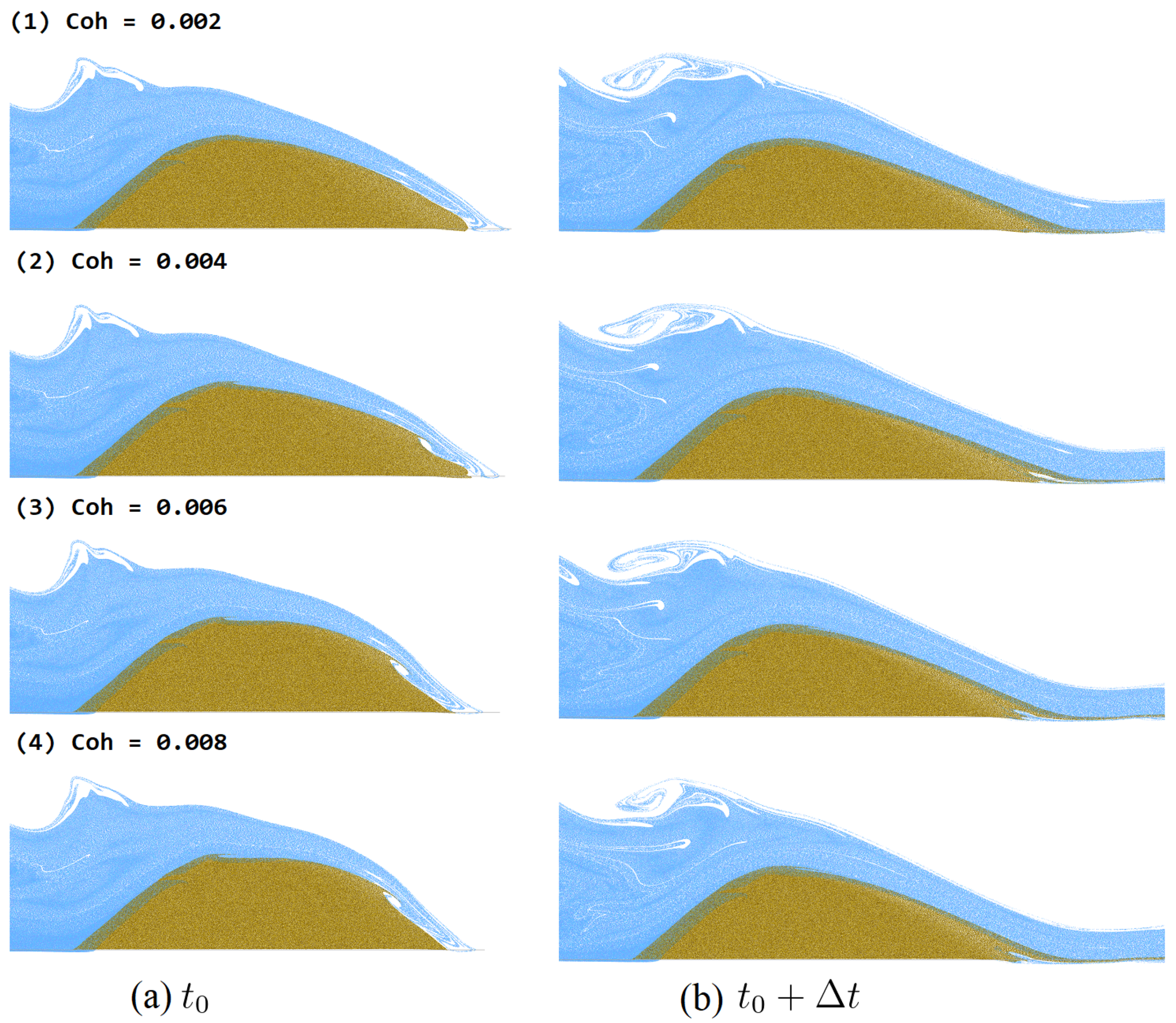
Parametric studies were conducted and are shown in Figure 4, Figure 5 and Figure 6 and Table 2. Figure 4 shows the different selection of the cohesion parameter from the range 0.002 to 0.008, which will have an influence on the overtopping dam breach erosion simulation. The result shows that with the higher cohesion demonstrated in Figure 4(4), the dam structure is more stable during the overtopping breach for the same timestamp. Especially on the right edge of the dam in Figure 4(4), the dam structure contains less shape deformation than the low cohesive dam structure at the same timestamp compared with Figure 4(3). The soil with a higher cohesion parameter for the earthen embankment homogeneous cohesive dam will maintain the dam structure from the overtopping dam breach.
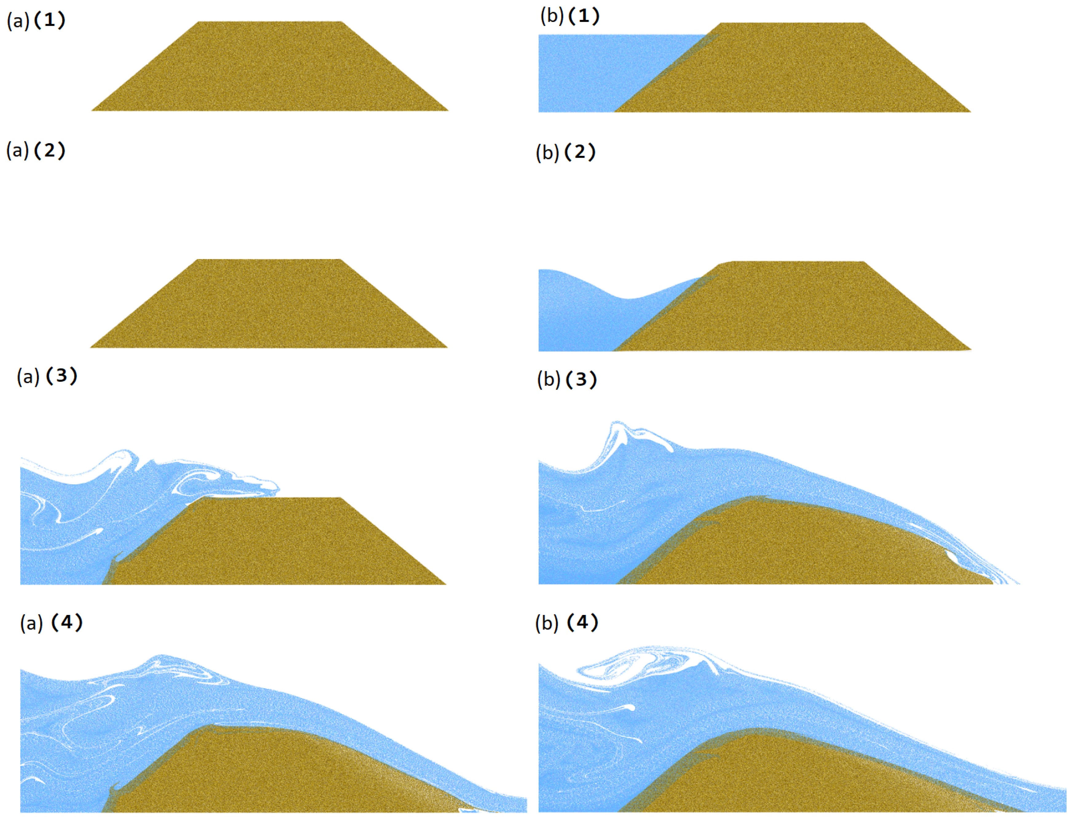
Figure 5 demonstrates two initial reservoir setups that will have an impact on the overtopping dam breach erosion along the downslope embankment. Figure 5(a1–a4) shows the empty initial reservoir overtopping the breach process at each timestamp. For Figure 5a, the quantified quantified parameters are shown in Table 2, Example 1. The initial reservoir level is zero meters, and the dam dimensions are a crest width of 6 m and a dam height of 3.75 m. Figure 5(b1–b4) shows the full reservoir overtopping breach process at each timestamp. For Figure 5b, the quantified parameters are shown in Table 2, Example 2. For Example 2, the initial reservoir level is 3.25 m, and the dam dimensions are a crest width of 6 m and a dam height of 3.75 m. The result clearly shows that the dam in Figure 5b experiences more erosion at the downward levee during the breach process.
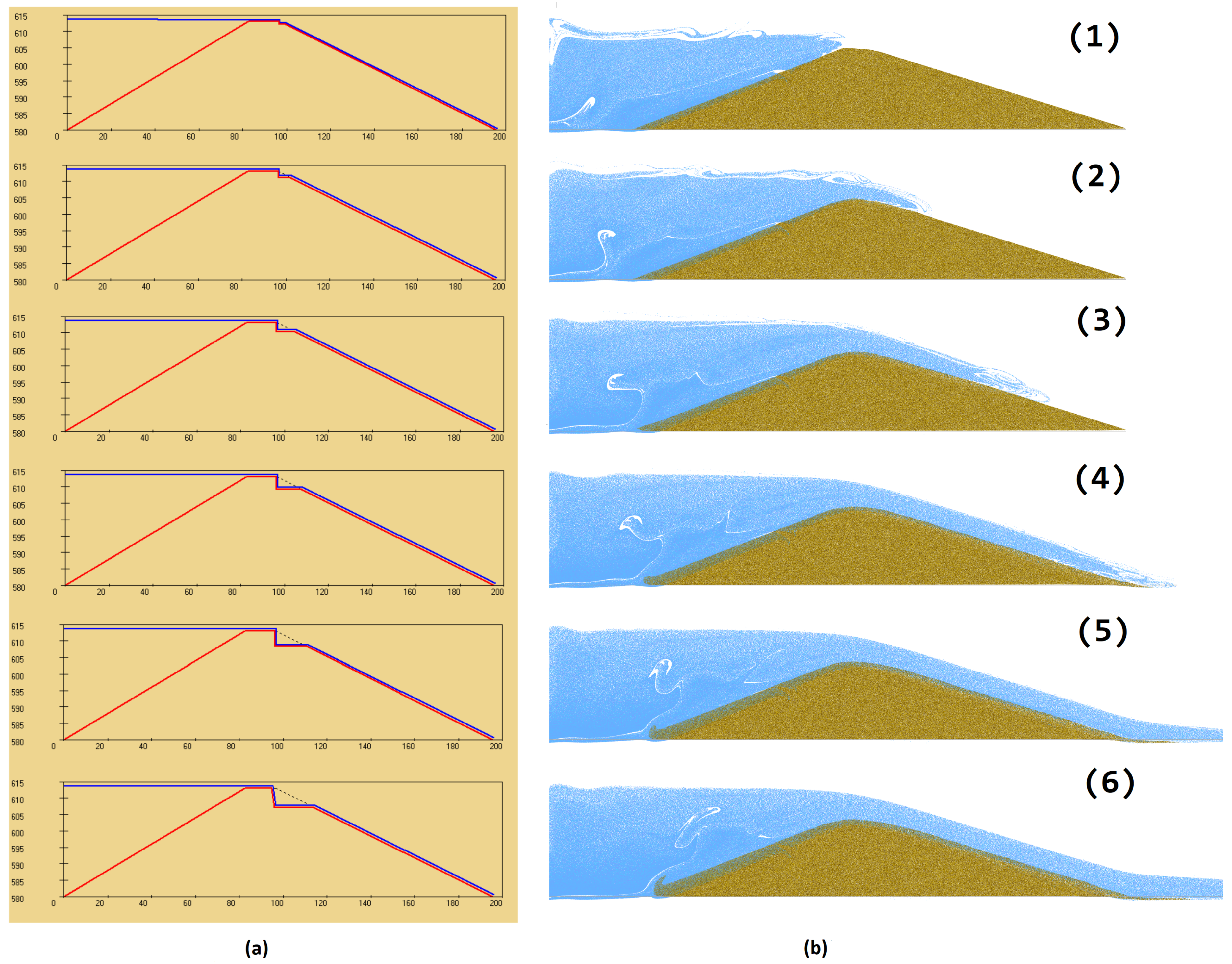
Furthermore, the WinDAM C [40] 05-HR-OBA example was applied to the proposed MPM simulation, and the comparison result is shown in Figure 6. WinDAM C [40] is a module used to analyze overtopping earth embankments. Figure 6a is the output from WinDAM C. Figure 6b is the simulation results using the proposed MPM simulation model. The parameter setting and condition for the cohesive dam overtopping failure cases are shown in Table 2. The dimension and dam structure specs are set up in the column 05-HR-OBA in Table 2. WinDAM C simulates the result using the same 05-HR-OBA example. As shown in Figure 6, from Figure 6a’s WinDAM output, the dam breach erosion process gradually deforms the right top edge of the dam crust. The physical-based erosion model used by WinDAM is the Hanson/Robinson stress-driven model [50]. Hanson/Robinson’s model assumes a vertical cut in a cohesive soil is located at a distance of half the bank height back from the edge. Furthermore, the head cut is made to advance through a series of mass failures driven by erosion at the base. Therefore, the model will erode the cohesive soil on the base surface and form a wedge-shaped notch.
In the proposed MPM simulation result in Figure 6b, the head cut during dam overtopping breach occurred progressively. As the saturation of the water and soil mixture reaches the critical point, the right downward levee starts to erode. The right bottom is enlarged due to the erosion and gradual soil movement, and the deformation shape of the dam head cut is not necessarily a wedge shape. Compared with the output from WinDAM C, it shows that the erosion deformation on the levee happens dramatically since WinDAM C uses the Hanson/Robinson stress-driven model, and in the proposed MPM simulation result, the erosion process occurred smoothly due to the MPM calculation based on the interaction between each particle and the surrounding grids. Table 2 also concludes about other dam failure examples simulated using the proposed method. It contains Samples 1 to 5, which are the samples shown in Figure 1, Figure 2, Figure 3, Figure 4 and Figure 5. HE1S1 is another physical-based experimental dam failure example tested by Hanson et al. [51].
Zhong et al. [52], Wu [53], and Hanson et al. [51] modeled the embankment breaching using a physical-based model. Wu’s [53] model approximates the breach caused by overtopping flow as a flat broad-crested weir with a trapezoidal cross-section. Zhong et al.’s [52] model formulates the breach evolution along the dam’s axis, as well as the head cut formation and migration in the longitudinal section. Hanson et al. [51] provided experimental data for future numerical model development. All these physical models contain mathematical equations and only work on the physical erosion model, and the simulation and visualization effects of erosion processes are not well considered. Nia et al. [8], Pu et al. [9], and Zhao et al. [54] used SPH or the MPM to simulate the dam break process, but they only talked about single-phase water. Tampubolon and Angeles [36] and Yan et al’s [55] study about the fluids’ and solids’ interaction mainly focused on the visualization results. Tampubolon and Angeles’ [36] MPM model and simulation achieved excellent results, but they lacked a comparison with real dam breach examples.
Based on the simulation results, the proposed MPM is able to provide extensive details during the erosion process on the levee and gives hydraulic scientists robust animated visualization results for the dam safety study. The proposed MPM also compares the existing physical model results using WinDAM. The MPM simulation model was developed to predict the overtopping breaching process of a cohesive dam. Unlike other large-scale physically-based dam breach models [52,53], the proposed MPM clearly illustrates the flow of soil sediment and water mixture. The performance of the 05-HR-OBA case shows that the proposed model gives rich details when the deformation is happening. Furthermore, the proposed MPM model can perform a parametric study, a synthetic study on cohesion, and compare a physical model.
4. Conclusions and Future Work
We propose a dam breach simulation framework using the material point method. Based on the simulation results, the proposed MPM can provide extensive details during the erosion process on the downward levee. We also compare the proposed simulation results with the existing physical-based model, WinDAM. For the current implementation, the model we use for the momentum exchange and energy density function is a simplified version, and it can be improved. Furthermore, the simulation time for the proposed MPM method is 60 s, but the simulation time for WinDAM C is around 16 h. For the current stage, the proposed MPM simulates the process in a shorter time. In a future study, we could implement the proposed simulation on a large scale and also try to implement the complete version of the momentum exchange and energy density function. By optimizing the experiment’s implementation, we hope we can achieve more experimental accuracy and reduce the run time at the same time.
Overall, our proposed simulation framework provides rich details during the dam breach process. Unlike simply considering the dam break removal part as a triangle in a physics-based model like WinDAM, the proposed framework can capture the water and soil interaction and gradually remove the soil during the breach process when simulating using the existing dam breach example.
Author Contributions
The authors contributed equally to this work. Both authors have read and agreed to the published version of the manuscript.
Funding
This research received no external funding.
Institutional Review Board Statement
Not applicable.
Informed Consent Statement
Not applicable.
Data Availability Statement
Data sharing is not applicable to this article.
Acknowledgments
The authors gratefully acknowledge the support of the USDA Hydraulic Engineering Laboratory in Stillwater, Oklahoma, USA, for providing the data and WinDAM software used in this study.
Conflicts of Interest
The authors declare no conflict of interest.
Sample Availability
Source code and data are available from the authors.
References
- Ozmen-Cagatay, H.; Kocaman, S. Dam-break flow in the presence of obstacle: Experiment and CFD simulation. Eng. Appl. Comput. Fluid Mech. 2011, 5, 541–552. [Google Scholar] [CrossRef] [Green Version]
- Biscarini, C.; Di Francesco, S.; Manciola, P. CFD modelling approach for dam break flow studies. Hydrol. Earth Syst. Sci. 2010, 14, 705–718. [Google Scholar] [CrossRef] [Green Version]
- Sina Hosseini Boosari, S. Predicting the Dynamic Parameters of Multiphase Flow in CFD (dam-break simulation) using artificial intelligence-(cascading deployment). Fluids 2019, 4, 44. [Google Scholar] [CrossRef] [Green Version]
- Neilsen, M.L. Computational Fluid Dynamics Models for WinDAM Computational Fluid Dynamics Models for WinDAM. In Proceedings of the 30th International Conference on Computers and their Applications, Honolulu, HI, USA, 9–11 March 2015. [Google Scholar]
- Cao, C.; Neilsen, M.L. Flexible Architecture for Analysis of Water Control Structures. In Proceedings of the International Conference On Computer Applications In Industry And Engineering, Las Vegas, NV, USA, 19–21 March 2018. [Google Scholar]
- De Leffe, M.; Le Touzé, D.; Alessandrini, B. SPH modeling of shallow-water coastal flows. J. Hydraul. Res. 2010, 48, 118–125. [Google Scholar] [CrossRef]
- Gong, K.; Shao, S.; Liu, H.; Wang, B.; Tan, S.K. Two-phase SPH simulation of fluid-structure interactions. J. Fluids Struct. 2016, 65, 155–179. [Google Scholar] [CrossRef] [Green Version]
- Nia, M.R.M.; Ghobadian, R.; Ahmadyan, S.; Ebrahimnejadian, H. Simulation of Dam Break Using Modified Incompressible Smoothed Particles Hydrodynamics (MPM-I-SPH). Int. J. Sci. Eng. Res. 2014, 5, 1051–1057. [Google Scholar]
- Pu, J.H.; Shao, S.; Huang, Y.; Hussain, K. Evaluations of swes and sph numerical modelling techniques for dam break flows. Eng. Appl. Comput. Fluid Mech. 2013, 7, 544–563. [Google Scholar] [CrossRef]
- Moreira, A.; Leroy, A.; Violeau, D.; Taveira-Pinto, F. Dam spillways and the SPH method: Two case studies in Portugal. J. Appl. Water Eng. Res. 2019, 9676. [Google Scholar] [CrossRef]
- Zhao, J.; Shan, T. Coupled CFD-DEM simulation of fluid-particle interaction in geomechanics. Powder Technol. 2013, 239, 248–258. [Google Scholar] [CrossRef]
- Shi, Z.M.; Zheng, H.C.; Yu, S.B.; Peng, M.; Jiang, T. Application of CFD-DEM to investigate seepage characteristics of landslide dam materials. Comput. Geotech. 2018, 101, 23–33. [Google Scholar] [CrossRef]
- Zhao, T.; Utili, S.; Crosta, G.B. Rockslide and Impulse Wave Modelling in the Vajont Reservoir by DEM-CFD Analyses. Rock Mech. Rock Eng. 2016, 49, 2437–2456. [Google Scholar] [CrossRef] [Green Version]
- Shan, T.; Zhao, J. A coupled CFD-DEM analysis of granular flow impacting on a water reservoir. Acta Mech. 2014, 225, 2449–2470. [Google Scholar] [CrossRef]
- Li, X.; Zhao, J. Numerical simulation of dam break by a coupled CFD-DEM approach. In Proceedings of the 15th Asian Regional Conference on Soil Mechanics and Geotechnical Engineering, ARC 2015: New Innovations and Sustainability, Kyushu, Japan, 9–13 November 2015; pp. 691–696. [Google Scholar] [CrossRef] [Green Version]
- Park, K.M.; Yoon, H.S.; Kim, M.I. CFD-DEM based numerical simulation of liquid-gas-particle mixture flow in dam break. Commun. Nonlinear Sci. Numer. Simul. 2018, 59, 105–121. [Google Scholar] [CrossRef]
- Rungjiratananon, W.; Szego, Z.; Kanamori, Y.; Nishita, T. Real-time Animation of Sand-Water Interaction. Comput. Graph. Forum 2008, 27. [Google Scholar] [CrossRef]
- Wu, K.; Yang, D.; Wright, N. A coupled SPH-DEM model for fluid-structure interaction problems with free-surface flow and structural failure. Comput. Struct. 2016, 177, 141–161. [Google Scholar] [CrossRef]
- Canelas, R. A generalized SPH-DEM discretization for the modelling of complex multiphasic free surface flows. arXiv 2013, arXiv:1011.1669v3. [Google Scholar] [CrossRef]
- Lenaerts, T.; Dutré, P. Mixing Fluids and Granular Materials; Blackwell Publishing Ltd.: Oxford, UK, 2009; Volume 28. [Google Scholar]
- Sulsky, D. A particle method for history-dependent materials. Comput. Methods Appl. Mech. Eng. 1994, 118, 179–196. [Google Scholar] [CrossRef]
- Soga, K.; Alonso, E.; Yerro, A.; Kumar, K.; Bandara, S.; Kwan, J.S.; Koo, R.C.; Law, R.P.; Yiu, J.; Sze, E.H.; et al. Trends in large-deformation analysis of landslide mass movements with particular emphasis on the material point method. Geotechnique 2018, 68, 457–458. [Google Scholar] [CrossRef] [Green Version]
- Troncone, A.; Conte, E.; Pugliese, L. Analysis of the slope response to an increase in pore water pressure using the material point method. Water 2019, 11, 1446. [Google Scholar] [CrossRef] [Green Version]
- Troncone, A.; Pugliese, L.; Conte, E. Run-out simulation of a landslide triggered by an increase in the groundwater level using the material point method. Water 2020, 12, 2817. [Google Scholar] [CrossRef]
- Yerro, A.; Alonso, E.E.; Pinyol, N.M. The material point method for unsaturated soils. Geotechnique 2015, 65, 201–217. [Google Scholar] [CrossRef] [Green Version]
- Yerro, A.; Alonso, E.E.; Pinyol, N.M. Run-out of landslides in brittle soils. Comput. Geotech. 2016, 80, 427–439. [Google Scholar] [CrossRef] [Green Version]
- Yerro, A.; Soga, K.; Bray, J. Runout evaluation of oso landslide with the material point method. Can. Geotech. J. 2019, 56, 1304–1317. [Google Scholar] [CrossRef] [Green Version]
- Conte, E.; Pugliese, L.; Troncone, A. Post-failure stage simulation of a landslide using the material point method. Eng. Geol. 2019, 253, 149–159. [Google Scholar] [CrossRef]
- Conte, E.; Pugliese, L.; Troncone, A. Post-failure analysis of the Maierato landslide using the material point method. Eng. Geol. 2020, 277, 105788. [Google Scholar] [CrossRef]
- Tran, Q.A.; Sołowski, W. Generalized Interpolation Material Point Method modelling of large deformation problems including strain-rate effects—Application to penetration and progressive failure problems. Comput. Geotech. 2019, 106, 249–265. [Google Scholar] [CrossRef]
- Dong, Y.; Wang, D.; Randolph, M.F. Investigation of impact forces on pipeline by submarine landslide using material point method. Ocean. Eng. 2017, 146, 21–28. [Google Scholar] [CrossRef]
- Dong, Y.; Wang, D.; Randolph, M.F. Quantification of impact forces on fixed mudmats from submarine landslides using the material point method. Appl. Ocean. Res. 2020, 102, 102227. [Google Scholar] [CrossRef]
- Ceccato, F.; Yerro, A. Modelling soil-water interaction with the Material Point Method. Evaluation of single-point and double-point formulations. In Proceedings of the 9th European Conference on Numerical Methods in Geotechnical Engineering (NUMGE 2018), Porto, Portugal, 25–27 June 2018. [Google Scholar]
- Bandara, S.; Ferrari, A.; Laloui, L. Modelling landslides in unsaturated slopes subjected to rainfall infiltration using material point method. Int. J. Numer. Anal. Methods Geomech. 2016, 1358–1380. [Google Scholar] [CrossRef]
- Bandara, S.; Soga, K. Coupling of soil deformation and pore fluid flow using material point method. Comput. Geotech. 2015, 63, 199–214. [Google Scholar] [CrossRef]
- Tampubolon, A.P.; Angeles, L. Multi-species simulation of porous sand and water mixtures. ACM Trans. Graph. 2017, 36, 1–11. [Google Scholar] [CrossRef]
- Klár, G.; Gast, T.; Pradhana, A.; Fu, C.; Schroeder, C.; Jiang, C.; Teran, J. Drucker-prager elastoplasticity for sand animation. ACM Trans. Graph. 2016, 35, 1–12. [Google Scholar] [CrossRef] [Green Version]
- Arduino, P.; Shin, W.; Moore, J.A.; Miller, G.R. Modeling strategies for multiphase drag interactions using the material point method. Int. J. Numer. Methods Eng. 2010, 295–322. [Google Scholar] [CrossRef]
- Jassim, I.; Stolle, D.; Vermeer, P. Two-phase dynamic analysis by material point method. Int. J. Numer. Anal. Methods Geomech. 2013, 37, 2502–2522. [Google Scholar] [CrossRef]
- Neilsen, M.L.; Hall, N. WinDAM: Earthen Embankment Erosion Analysis WinDAM: Earthen Embankment Erosion Analysis. In Proceedings of the 24th International Conference on Computers and Their Applications in Industry and Engineering (CAINE-2011), Honolulu, HI, USA, 16–18 November 2011. [Google Scholar]
- Atktn, B.R.J.; Craine, R.E. Continuum theories of mixtures: Basic theory and historical development. Q. J. Mech. Appl. Math. 1976, 29, 209–244. [Google Scholar]
- Borja, R.I. On the mechanical energy and effective stress in saturated and unsaturated porous continua. Int. J. Solids Struct. 2006, 43, 1764–1786. [Google Scholar] [CrossRef] [Green Version]
- Bonet, J.; Wood, R.D. Nonlinear Continuum Mechanics for Finite Element Analysis, 2nd ed.; Cambridge University Press: Cambridge, UK, 2008. [Google Scholar] [CrossRef] [Green Version]
- Drucker, D.C.; Prager, W. Soil mechanics and plastic analysis or limit design. Q. Appl. Math. 1943, 10, 157–165. [Google Scholar] [CrossRef] [Green Version]
- Becker, M. Weakly compressible SPH for free surface flows. In Proceedings of the 2007 ACM SIGGRAPH/Eurographics Symposium on Computer Animation, San Diego, CA, USA, 2–4 August 2007; pp. 1–8. [Google Scholar]
- Robert, K.D. Soil-Pipeline Interaction in Unsaturated Soils. Ph.D. Thesis, University of Cambridge, Cambridge, UK, 2010. [Google Scholar]
- Jiang, C.; Selle, A.; Teran, J. The Affine Particle-In-Cell Method. ACM Trans. Graph. 2015, 34, 1–10. [Google Scholar] [CrossRef]
- Stomakhin, A.; Schroeder, C.; Chai, L.; Teran, J.; Selle, A. A material point method for snow simulation. ACM Trans. Graph. 2013, 32, 1–10. [Google Scholar] [CrossRef]
- Xia, Y.; Ge, Z.; Chen, Y.; Liu, B.; Huang, Z. Flame; GitHub Repository. 2018. Available online: https://github.com/YiYiXia/Flame (accessed on 19 January 2020).
- Hanson, G.J.; Robinson, K.M.; Cook, K.R. Prediction of Headcut Migration Using a Deterministic Approach. Trans. ASAE 2001, 44, 525–531. [Google Scholar] [CrossRef]
- Hanson, G.J.; Cook, K.R.; Hunt, S.L. Physical Modeling of Overtopping Erosion and Breach Formation of Cohesive Embankments. Trans. ASAE 2005, 48, 1783–1794. [Google Scholar] [CrossRef]
- Zhong, Q.M.; Chen, S.S.; Deng, Z.; Mei, S.A. Prediction of Overtopping-Induced Breach Process of Cohesive Dams. J. Geotech. Geoenvironmental Eng. 2019, 145. [Google Scholar] [CrossRef]
- Wu, W. Simplified physically based model of earthen embankment breaching. J. Hydraul. Eng. 2013, 139, 837–851. [Google Scholar] [CrossRef]
- Zhao, X.; Liang, D.; Martinelli, M. Numerical Simulations of Dam-break Floods with MPM. Procedia Eng. 2017, 175, 133–140. [Google Scholar] [CrossRef]
- Yan, X.; Li, C.F.; Chen, X.S.; Hu, S.M. MPM simulation of interacting fluids and solids. Comput. Graph. Forum 2018, 37, 183–193. [Google Scholar] [CrossRef]
Figure 1.
Overtopping dam breach simulation.

Figure 2.
(a) Deformation of a material. (b) Multi-phase deformation combining water and soil.

Figure 3.
The Material Point Method (MPM) algorithm with two grid multi-species. 1. (a)->(b) Transfer to grids: the mass and momentum of each species are transferred to its corresponding grid. 2. (b)->(c) Update the grids’ momentum: the coupled water and soil grid velocities are updated. 3. (c)->(d) Update the particles: all particle states, including the momentum, velocity, and cohesion based on saturation, are updated.

Figure 4.
Overtopping dam breach simulation with different cohesion at timestamps (a) and (b) .

Figure 5.
The overtopping dam breach simulation with an empty (a) and full (b) reservoir at different timestamps ((1)–(4)).
Figure 5.
The overtopping dam breach simulation with an empty (a) and full (b) reservoir at different timestamps ((1)–(4)).

Figure 6.
WinDAM C 05-HR-OBA (a) and the proposed MPM simulation (b) method comparison.


Table 1.
Glossary.
| Variable | Meaning |
|---|---|
| I | identity matrix |
| a | soil and water |
| t | time step size |
| material derivative | |
| density | |
| g | gravitational constant |
| drag coefficient | |
| weight | |
| weight gradient | |
| Particle | |
| h initial particle volume | |
| particle mass | |
| particle position | |
| particle velocity | |
| soil elastic deformation gradient | |
| soil plastic deformation gradient | |
| water determinant deformation gradient | |
| water saturation | |
| cohesion | |
| volume correction scalar | |
| Grid | |
| grid velocity | |
| grid node mass | |
| grid node location | |
| mixed water saturation on grid |
Table 2.
Condition for the cohesive dam’s overtopping failure cases and simulation cases.
| Dam Failure Example | 1 | 2 | 3 | 4 | 5 | HE1S1 | 05-HR-OBA | 05-HR-OBB |
|---|---|---|---|---|---|---|---|---|
| Cohesion | 0.01 | 0.008 | 0.006 | 0.004 | 0.002 | 0.008 | 0.008 | 0.008 |
| Gravity (m/s) | 3 | 3 | 3 | 3 | 3 | 3 | 9.8 | 9.8 |
| Initial Reservoir Level (m) | No | 3.25 | 3.25 | 3.25 | 3.25 | 4 | 2.4 | 2.4 |
| Number of Water Particles | 0 | 197,542 | 197,542 | 197,542 | 197,542 | 195,811 | 95,131 | 95,131 |
| Dam Height (m) | 3.75 | 3.75 | 3.75 | 3.75 | 3.75 | 4.6 | 3.3 | 3.3 |
| Crest Width (m) | 6 | 6 | 6 | 6 | 6 | 3.68 | 1 | 1 |
| Upstream Slope V/H | 0.8333 | 0.8333 | 0.8333 | 0.8333 | 0.8333 | 0.3333 | 0.3882 | 0.3882 |
| Downstream Slope V/H | 0.8333 | 0.8333 | 0.8333 | 0.8333 | 0.8333 | 0.3333 | 0.3143 | 0.3143 |
| Number of Soil Particle | 277,887 | 277,887 | 277,887 | 277,887 | 277,887 | 403,225 | 173,982 | 173,982 |
| Water Inlet Height (m) | 7.25 | 7.25 | 7.25 | 7.25 | 7.25 | 7.25 | 2.5 | 2.5 |
| Inlet Velocity (m/s) | 2 | 2 | 2 | 2 | 2 | 2 | 5 | 2 |
| Resolution | 7000 × 2800 | 7000 × 2800 | 7000 × 2800 | 7000 × 2800 | 7000 × 2800 | 7000 × 2800 | 7000 × 2800 | 7000 × 2800 |
| Number of Iterations | 2399 | 2185 | 1503 | 2399 | 1979 | 2399 | 2087 | 2371 |
| Simulation Time (h) | 44 | 50 | 30 | 55 | 42 | 71 | 64 | 43 |
Publisher’s Note: MDPI stays neutral with regard to jurisdictional claims in published maps and institutional affiliations. |
© 2021 by the authors. Licensee MDPI, Basel, Switzerland. This article is an open access article distributed under the terms and conditions of the Creative Commons Attribution (CC BY) license (http://creativecommons.org/licenses/by/4.0/).
Share and Cite
MDPI and ACS Style
Cao, C.; Neilsen, M. Dam Breach Simulation with the Material Point Method. Computation 2021, 9, 8. https://0-doi-org.brum.beds.ac.uk/10.3390/computation9020008
AMA Style
Cao C, Neilsen M. Dam Breach Simulation with the Material Point Method. Computation. 2021; 9(2):8. https://0-doi-org.brum.beds.ac.uk/10.3390/computation9020008
Chicago/Turabian StyleCao, Chendi, and Mitchell Neilsen. 2021. "Dam Breach Simulation with the Material Point Method" Computation 9, no. 2: 8. https://0-doi-org.brum.beds.ac.uk/10.3390/computation9020008
Note that from the first issue of 2016, this journal uses article numbers instead of page numbers. See further details here.