
Transient Pressure-Driven Electroosmotic Flow through Elliptic Cross-Sectional Microchannels with Various Eccentricities


1
Applied Mathematics Program, Faculty of Science and Technology, Valaya Alongkorn Rajabhat University under the Royal Patronage, Pathum Thani 13180, Thailand
2
Department of Mathematics, Faculty of Science, Ramkhamhaeng University, Bangkok 10240, Thailand
*
Author to whom correspondence should be addressed.
†
These authors contributed equally to this work.
Computation 2021, 9(3), 27; https://0-doi-org.brum.beds.ac.uk/10.3390/computation9030027
Submission received: 31 January 2021
/
Revised: 21 February 2021
/
Accepted: 24 February 2021
/
Published: 1 March 2021
(This article belongs to the Special Issue Proceedings of the International Conference in Mathematics and Applications 2020_Mahidol University)
Abstract
:The semi-analytical solution for transient electroosmotic flow through elliptic cylindrical microchannels is derived from the Navier-Stokes equations using the Laplace transform. The electroosmotic force expressed by the linearized Poisson-Boltzmann equation is considered the external force in the Navier-Stokes equations. The velocity field solution is obtained in the form of the Mathieu and modified Mathieu functions and it is capable of describing the flow behavior in the system when the boundary condition is either constant or varied. The fluid velocity is calculated numerically using the inverse Laplace transform in order to describe the transient behavior. Moreover, the flow rates and the relative errors on the flow rates are presented to investigate the effect of eccentricity of the elliptic cross-section. The investigation shows that, when the area of the channel cross-sections is fixed, the relative errors are less than 1% if the eccentricity is not greater than 0.5. As a result, an elliptic channel with the eccentricity not greater than 0.5 can be assumed to be circular when the solution is written in the form of trigonometric functions in order to avoid the difficulty in computing the Mathieu and modified Mathieu functions.
1. Introduction
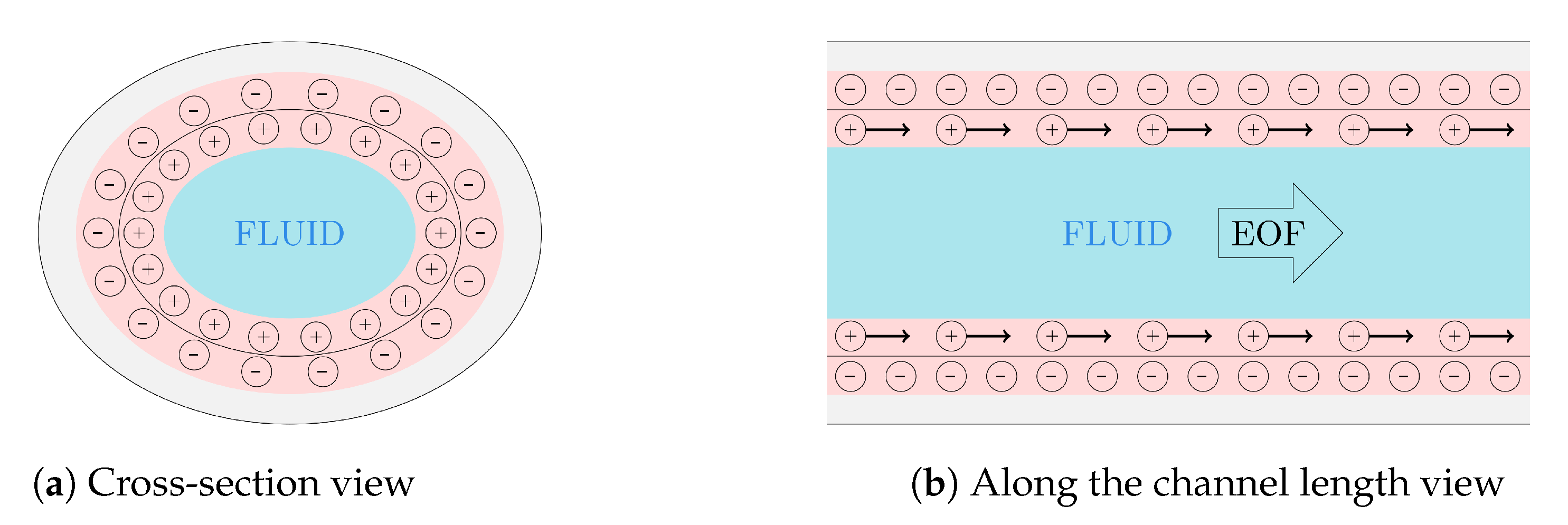
A manipulation on fluid flow under a microscale system has been studied intensively worldwide over the past decades [1,2,3,4,5,6] due to the utility of its applications in various fields; for example, lab-on-the-chips, portable medical devices, drug delivery devices and computer chips. One key to success in controlling fluid behavior through a very small scale channel is to employ an application of the well-known electrokinetic phenomenon, namely electroosmosis. Electroosmosis is a phenomenon of the fluid movement through a channel by the electrokinetic force, which relies on two layers of ions [7]. The first layer is the ions on the inner wall surface of the channel due to the chemical reaction between the channel surface and the fluid. The second layer is the counterions in the fluid adjacent to the channel wall as a result of the electrokinetic force from the first layer. The formation of these two electrical layers is called the electrical double layer (EDL) shown by red highlighted area in Figure 1. An application of an external electric field to the channel leads to a movement of the counterions in the fluid by electrokinetic force called as electroosmotic force. Therefore, the fluid flow in consequence of the drag force from the moving counterions induced by electroosmotic force is named as electroosmotic flow (EOF).
Since EDL locates on the interface of the channel and the fluid, the cross-sectional shape of cylindrical channel plays an important role on the fluid behavior [8]. Recently, understanding of fluid behavior through microchannels has been achieved using both experimental and theoretical studies [9,10,11,12,13,14]. In literature, the channels are considered as cylindrical microtubes with various cross-sections including rectangles [15,16], circles [17,18], annuli [19,20], ellipses [21,22] and other complex shapes [21,23], according to the occurrences of microfluidic applications.
With regard to the shape of many microfluidic devices and natural systems such as the vascular system, elliptic cylindrical geometry is considered to be the channel in many researches [21,22,24,25,26] in order to study the behavior of electroosmotic flow. However, the solution for fluid velocity through an elliptic cylindrical channel using the mathematical methodology is obtained in the form of Mathieu functions [22] which have difficulty in numerically computing its value due to the convergence of the function [27]. In 2015, Liu et al. [28] studied the effect of eccentricity on pure electroosmotic flow through an elliptic channel. Pressure-driven force was neglected and the flow was considered to be fully developed which means the transient behavior was omitted. Furthermore, the effect of eccentricity was investigated only when the circumference of the channel cross-section was fixed.
Therefore, in this study, we derive the solution for transient combined electroosmotic and pressure-driven flow through an elliptic cylindrical microchannel. The governing equation for fluid velocity is written in the homogeneous linear partial differential equation depending on both and in the elliptic coordinates. By employing the Laplace transform to eliminate the time-derivative term in the governing equation, the solution is obtained as the function of and . As a consequence, the solution is capable of describing the electroosmotic flow in the system when the boundary condition is either constant or varied on , which normally occurs in an elliptic cross-sectional microchannel [4,21,22,29,30]. However, the solution of the Laplace transform which is in the form of the special functions namely the Mathieu and modified Mathieu functions has complexity to find the inverse Laplace transform analytically. Thus, the numerical inverse Laplace transform is employed to yield the semi-analytical solution. This semi-analytical solution for transient electroosmotic flow allows us to investigate behavior of electroosmotic flow directly via the expression of the solution and takes an advantage of making the problem tractable for variations of domain and boundary condition which provide more efficiency (speed and accuracy) in computing the numerical results compared to the traditional numerical method. Moreover, the velocity profiles of the fluid flow are calculated numerically from the semi-analytical solution in order to demonstrate the transient behavior of electroosmotic flow. The effect of eccentricity of the elliptic channel on flow characteristics including the velocity profile, the volumetric flow rate and the relative error on the volumetric flow rate is investigated with two aspects: the circumference of the channel cross-section is fixed and the area of the channel cross-section is fixed.
2. Preliminaries on the Elliptic Coordinate System
2.1. Elliptic Coordinate System
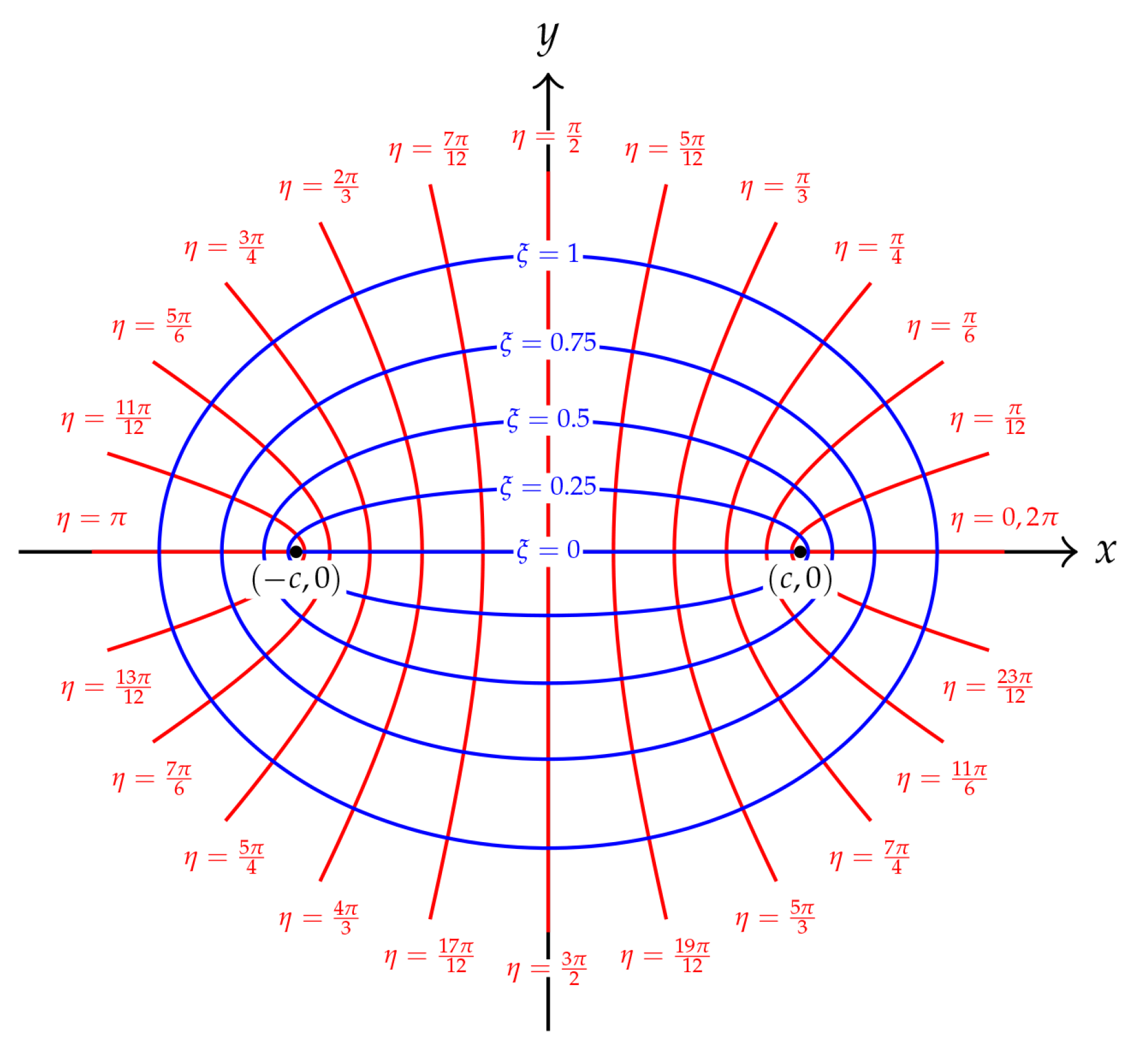
The elliptic coordinate system for an elliptic geometry with two foci at and of the Cartesian coordinate system is an orthogonal coordinate system in which represents the confocal ellipses and represents the confocal hyperbolas. The elliptic coordinates can be illustrated as shown in Figure 2.
The elliptic coordinates are defined by
where and . The identities of the elliptic coordinates related to the Cartesian coordinates are
and the Laplacian in the elliptic coordinates is
2.2. Mathieu Functions
Consider the 2-dimensional wave equation in the elliptic coordinates
By substituting and the identity
we can split Equation (6) into two second order ordinary differential equations as follows:
where a is the separation constant and . The solutions of the ordinary differential Equations (8) and (9) are written in the form of two special functions introduced by French mathematician, Émile Léonard Mathieu in 1868 [31]. The special functions are called as the Mathieu functions and modified Mathieu functions. Combining the solutions of Equations (8) and (9), we obtain the solution of Equation (6) as
where cem(η;q),sem(η;q) are the periodic Mathieu functions;
Cem(η;q),Sem(η;q) are the periodic modified Mathieu functions cem(η;q),sem(η;q), respectively;
Fem(η;q),Gem(η;q) are the non-periodic modified Mathieu functions cem(η;q),sem(η;q), respectively.
The coefficients and are functions depending solely on q, and the integer m denotes the order of the Mathieu and modified Mathieu functions. The formula of the above special functions can be found in [27].
According to the elliptic coordinate system , where represents the confocal hyperbolas defined on , the symmetric properties of the periodic Mathieu functions and can be derived as follows:
- is symmetrical about both x- and y-axes,
- is symmetrical about x-axis but antisymmetrical about y-axis,
- is antisymmetrical about x-axis but symmetrical about y-axis,
- is antisymmetrical about both x- and y-axes,
for all integer . Moreover, the orthogonality of the periodic Mathieu functions is
3. Mathematical Modeling
3.1. Electroosmotic Force
The electroosmotic force is given by
where E denotes the applied external electric field and denotes the ionic charge density which can be expressed by the Poisson-Boltzmann equation as follows:
where denotes the potential inside the channel, denotes the ionic concentration at the bulk, denotes the charge of a proton, denotes the valence of the ions in the fluid, denotes the permittivity of the fluid, is the Boltzmann constant, and T denotes the absolute temperature.
If the potential has low value, we can simplify Equation (15) by using to be the well-known Debye-Hückel approximation in the elliptic coordinates as
where represents the reciprocal of the EDL thickness. Combining Equations (14)–(16), we can write the electroosmotic force related to the potential as
Since Equation (16) is in the form of Equation (6), the general solution is obtained in the similar form as follows:
where and are constant with .
According to the symmetric property of an elliptic geometry, the potential is supposed to be symmetrical about both x- and y-axes. Hence, we can express the boundary conditions of in the elliptic coordinate system by the following equations:
The general solution shown in Equation (18) can be reduced, according to the symmetric property of the potential , as follows:
Since the partial derivative of the modified Mathieu function with respect to does not vanish when [27], the constant has to be zero in order to satisfy the boundary condition (21). Therefore, the general solution (22) is reduced to
where . Moreover, if the potential at the wall surface is determined by the function , we can write the boundary of the potential at the boundary of the elliptic channel as
3.2. Fluid Velocity
Suppose that the fluid flow does not swirl, we can describe the fluid behavior of electroosmotic flow through an elliptic cylindrical microchannel along z-axis by the Navier-Stokes equations with the electroosmotic force in the elliptic cylindrical coordinate system as shown:
where denotes the fluid velocity in z-direction, denotes the fluid density, denotes the fluid viscosity, and denotes the constant pressure gradient in z-direction. Substituting the term of electroosmotic force in Equation (26) with the relation in Equation (17) yields
To eliminate the time-derivative, we employ the Laplace transform defined by
and the initial condition . Therefore, Equation (27) becomes
which has the general solution written in the form of
where is the complementary solution (homogeneous solution), is the particular solution corresponding to non-homogeneous term , and is the particular solution corresponding to non-homogeneous term .
For the complementary solution , we consider the homogeneous equation
Since Equation (31) is in the form of Equation (6), the complementary solution is obtained in the similar form as follows:
where , and are constant with .
For the particular solution , since the non-homogeneous term does not depend on both and , we can assume that is constant. By the method of undetermined coefficients, we obtain as follows:
For the particular solution , since the non-homogeneous term is in the form of the Mathieu and modified Mathieu functions shown in Equation (23), we assume that the particular solution is also in the same formula as
Since is the particular solution of the corresponding non-homogeneous equation
we have
Moreover, substituting Equation (23) into Equation (16) and equating the term having the function with the same integer m, then we obtain
for all integer . Observe that -4.6cm0cm
we can rewritten Equation (36) as
By equating coefficients of the terms having the same order of the periodic Mathieu function , we can derive the constant for the particular solution from
for all integer .
Similarly to the potential , we also suppose that v is symmetrical about both x- and y-axes. Therefore, the solution in Equation (41) is reduced to
In this study, we consider the no-slip condition of the fluid, that is, which implies
As a result, the constant can be determined using the orthogonality of the Mathieu function by
for all integer , where
The fluid velocity u can be obtained by employing the inverse Laplace transform as follows:
where is a number that is greater than the real part of all singularities of in the complex s-plane.
For steady flow, the time-derivative of the fluid velocity is vanished. Therefore, Equation (26) with the relation in Equations (14) and (15) can be reduced to
where u is now the function depending only on and . Let
We can rewrite Equation (47) by using the identity in Equation (7) to be the Laplace equation of the function as
Using the method of separation of variables, we obtain
where is constant. Substituting the general solution into Equation (48) yields
where the constant can be derived from the no-slip condition with the orthogonality of the trigonometric functions as
4. Numerical Results
In this section, we employ the numerical inverse Laplace transform on the general solution of fluid velocity as shown in Equation (42) in order to investigate the behavior of transient electroosmotic flow through an elliptic cylindrical microchannel. The calculation of , , and is presented in Appendix A. The dimensions of the elliptic cross-section, the fluid properties [8] and the other parameters used in the investigation are presented in Table 1.
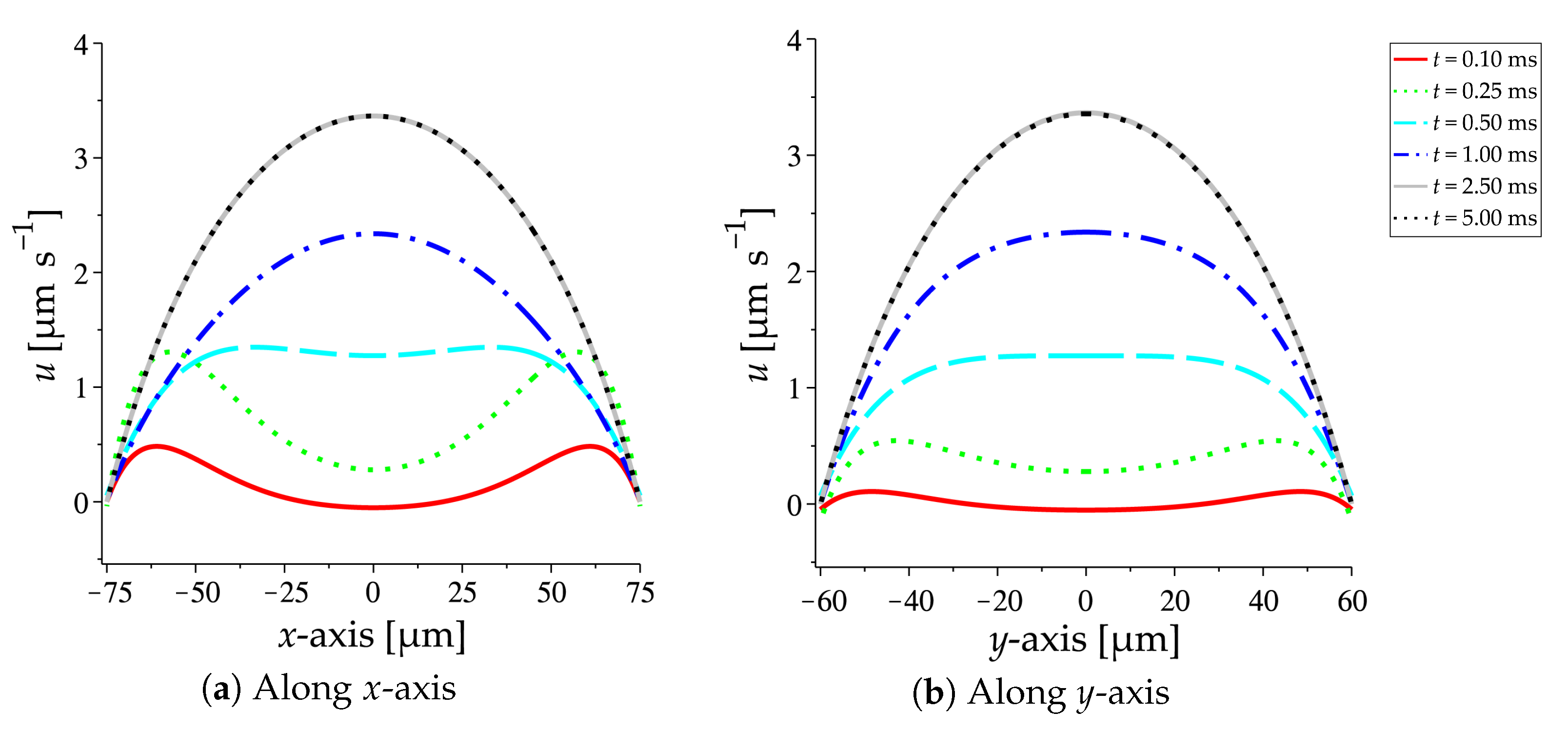
Figure 3 illustrates the velocity profiles of transient flow along both x- and y-axes. The results show that the flow develops only from the area adjacent to the wall at the beginning time and represented by the red and green lines, respectively. This is due to the effect of the moving ions in the fluid within the electrical double layers. However, at time , represented by the cyan line, the flow at the center of the channel starts developing. The flow becomes fully developed at time , which represented by the gray line.
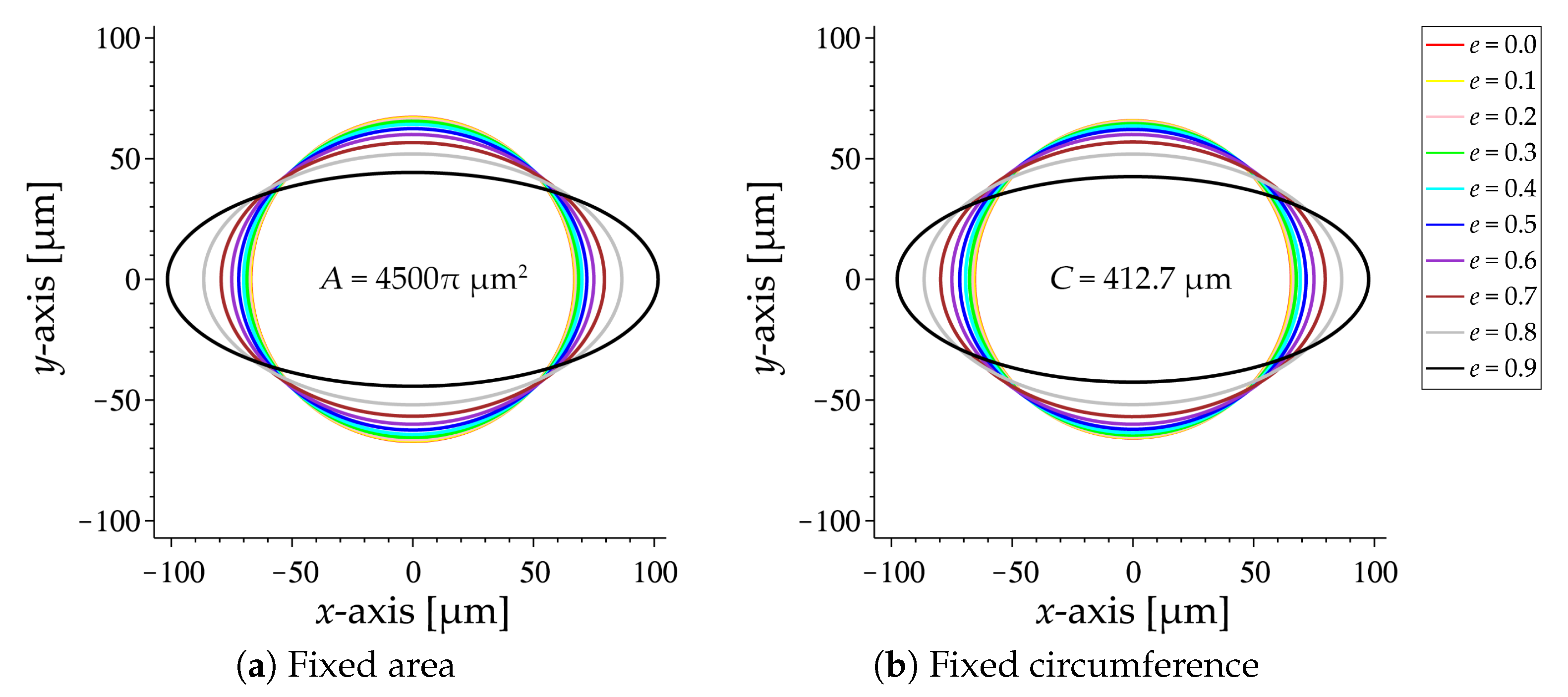
After fully developing, the flow becomes steady. As a result, we use the velocity of steady flow shown in Equation (51) to investigate the effect of eccentricity on fluid flow through the elliptic channel. The eccentricity of ellipses varies from 0 (circle) to 0.9 by increment of 0.1. The variation of the elliptic cross-sections of the channel on various eccentricities is presented in Figure 4.
The investigation on the effect of eccentricity consists of two parts. For the first part, we fix the area A of all ellipses to be 4500 (see Figure 4a). This value is obtained by calculating the area of the ellipse having the parameters as shown in Table 1. Then, for each eccentricity, we can calculate the focal length c and the boundary of the ellipse as follows:
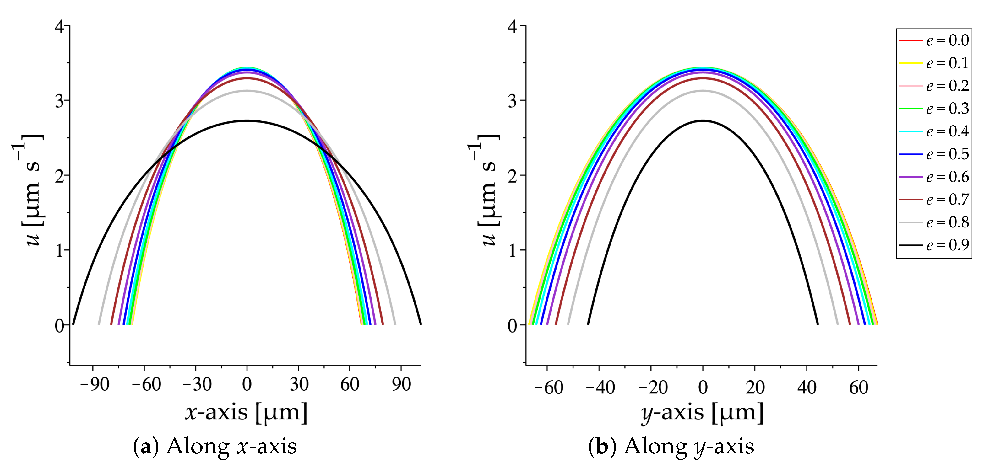
Figure 5 presents the comparison of the velocity profiles of electroosmotic flow through the elliptic channel with various eccentricities when the area is fixed. The velocity profiles along x- and y-axes are shown in Figure 5a,b, respectively. The results show that there is no significant difference for the velocity profiles along both x- and y-axes in the channels with the eccentricity between 0 and 0.6. However, when the eccentricity is greater than 0.6, the velocity drops along the entire x- and y-axes as an increase of the eccentricity.
For the second part, we fix the circumference C of all ellipses equal to about 412.7 (see Figure 4b). This value is also obtained by calculating the circumference of the ellipse having the parameters as shown Table 1. Then, for each eccentricity, we can calculate the boundary of the ellipse by Equation (54) and the focal length c as
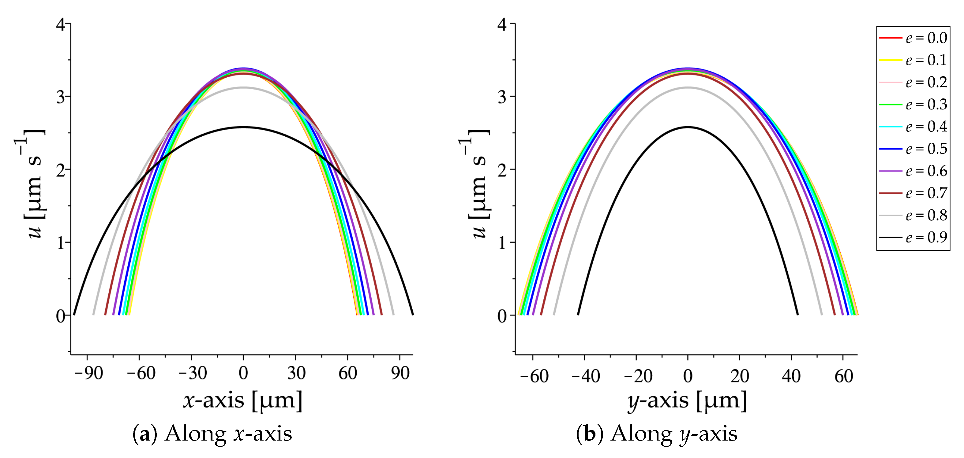
Figure 6 presents the comparison of the velocity profiles of electroosmotic flow through the elliptic channel with various eccentricities when the circumference is fixed. The velocity profiles along x- and y-axes are shown in Figure 6a,b, respectively. The results show that the pattern of the velocity profiles is quite similar compared to the one when the area is fixed. Indeed, the velocity profiles are not significantly different when the eccentricity is between 0 and 0.6. However, the velocity decreases along the entire x- and y-axes as an increase of the eccentricity when the eccentricity is greater than 0.6.
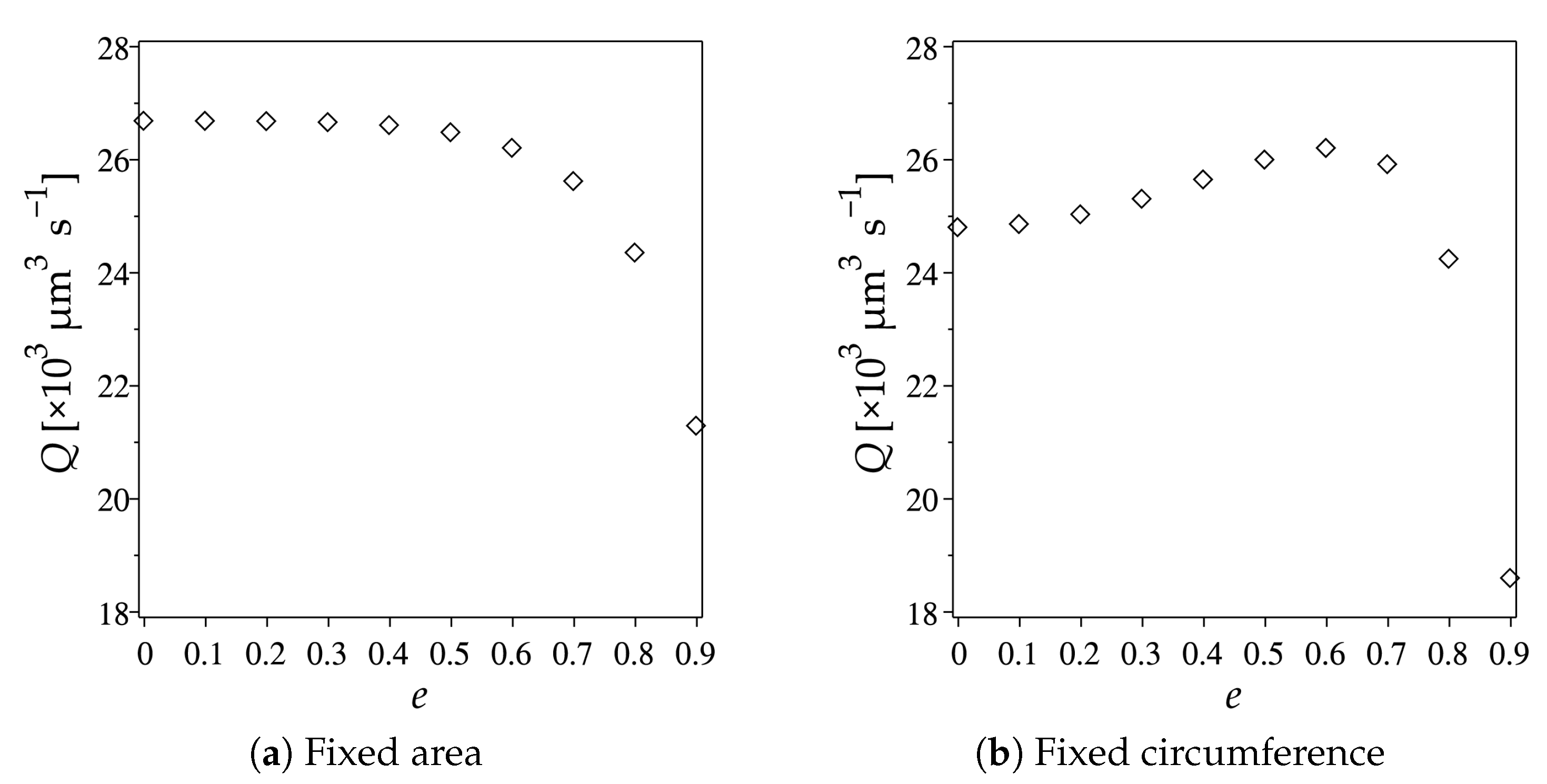
Since the efficiency of flow control in microfluidics mainly relies on the accuracy of flow rate, we also investigate the effect of eccentricity on the volumetric flow rate Q of the fluid through the elliptic cylindrical microchannel. The flow rates can be calculated by integrating the fluid velocity of steady flow, shown in Equation (51), over the cross-sectional area. Therefore, the formula of the flow rate is expressed as
Figure 7 demonstrates the comparison of the flow rates calculated when the area (see Figure 7a) and the circumference (see Figure 7b) of ellipse are fixed by using the parameters from the first and the second parts of the investigation on the fluid velocity, respectively. The results show that, when the area is fixed, there is no significant difference for the flow rate in the channels with the eccentricity between 0 and 0.5. When the eccentricity is greater than 0.5; however, the flow rate decreases rapidly as the eccentricity increases. On the other hand, when the circumference is fixed, the flow rate increases significantly when the eccentricity is between 0.2 and 0.6 but the flow rate decreases dramatically when the eccentricity is greater than 0.6.
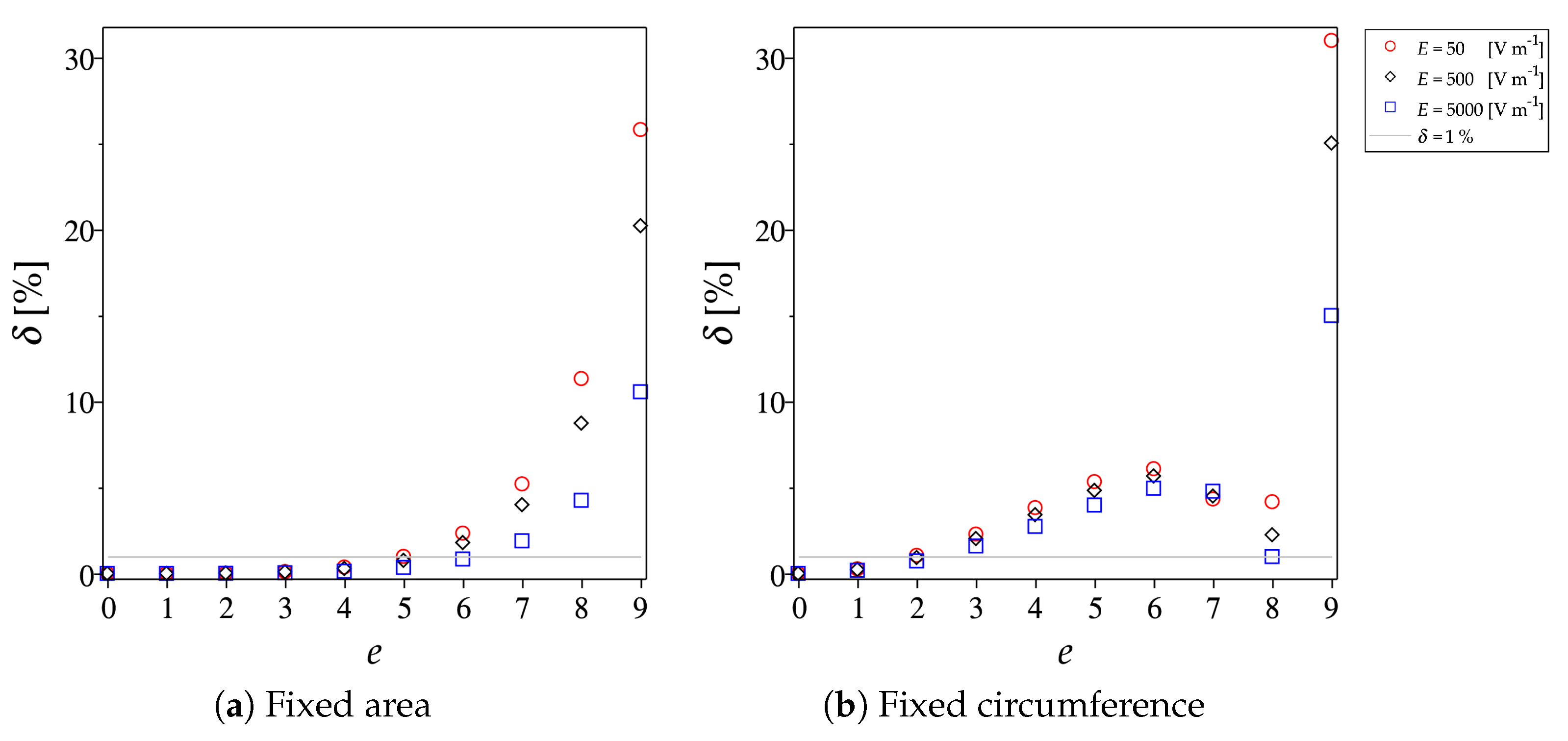
Furthermore, we define the relative error of the flow rate by
where is the flow rate with the eccentricity equal i. The comparison of the relative errors of the flow rates is presented in Figure 8 when the area and the circumference of the ellipse are fixed (Figure 8a,b, respectively). In addition, to investigate the effect of external electric field on the relative error, we consider the variation of the external electric field on the electroosmotic flow to be 0.1 and 10 times of the value shown in Table 1. Indeed, we investigate the relative error using the three different values of the external electric field and 5000 , respectively.
The results show that, when the area is fixed, the relative errors of all three cases are less than 1% in the channel with the eccentricity not greater than 0.5. However, when the eccentricity is greater than 0.5, the relative errors increase sharply as an increase of the eccentricity. On the other hand, when the circumference is fixed, the relative errors are less than 1% if the eccentricity is not greater than 0.2. However, there is a fluctuation in the relative errors with the value greater than 1% when the eccentricity is greater than 0.2. Moreover, the results show that, in all three cases, the relative errors increase as a decrease of the external electric field.
Since the relative error defined by Equation (57) can be used to describe the error of the flow rate in the elliptic channel when we consider it as the circular channel. Therefore, the results in Figure 8 also show that the consideration of an elliptic channel as the circular channel with the same circumference of the cross-section may cause high error in the flow rate which is inappropriate to use for any investigation. This influence of eccentricity agrees with that of Liu [28].
However, this study reveals a significant result that, when the area of cross-section is fixed, we can assume that the elliptic channel with the eccentricity not greater than 0.5 to be the circular channel. This assumption can be used to avoid the difficulty in computing the velocity solution for electroosmotic flow in the elliptic channel, which is in the form of the Mathieu and modified Mathieu functions. Moreover, it provides a simpler way to further the numerical investigation of electroosmotic flow in some elliptic systems.
5. Conclusions
In this study, we present the semi-analytical solution for transient pressure-driven electroosmotic flow through elliptic cylindrical microchannels based on the Mathieu and modified Mathieu functions. The velocity profiles of transient pressure-driven electroosmotic flow are calculated numerically in order to investigate the transient behavior. Moreover, the variations of the fluid velocities, the flow rates and the relative errors of the flow rates with various eccentricities of the channel cross-section are presented to investigate the effect of eccentricity of the elliptic cross-sectional microchannel. The results show that the elliptic channel with the eccentricity not greater than 0.5 can be considered as the circular channel with the same area of the cross-section to avoid the difficulty in numerically computing the solution for fluid velocity in the elliptic channel, which is based on the Mathieu and modified Mathieu functions. In addition, this assumption provides a simpler way of furthering numerical investigation of electroosmotic flow in some elliptic systems.
Author Contributions
Both authors contributed equally to this work. All authors have read and agreed to the published version of the manuscript.
Funding
This research received no external funding.
Institutional Review Board Statement
Not applicable.
Informed Consent Statement
Not applicable.
Data Availability Statement
Data sharing is not applicable to this article.
Conflicts of Interest
The authors declare no conflict of interest.
Appendix A
The procedure to calculate the Mathieu and modified Mathieu functions including , , and , which are in the formula of the solution, is presented as follows [27]:
For and integer , the functions , , and can be expressed by
To find the coefficients , substituting Equation (A1) into Equation (8) and equating the coefficients of the term for each yield the following recurrence relations:
where is the separation constant a corresponding to . Dividing Equations (A5) and (A6) by and Equation (A7) by , we obtain
where
Substituting from Equation (A12) into Equation (A15), we can calculate by solving the following equation:
Since as , we suppose for all provided R is large enough. Then can be obtained by solving the recurrence relations (A12)–(A14). The normalization of by
yields
or
It should be noted that the values of by the above procedure can be use for all of the functions , , and .
References
- Beskok, A.; Korniadakis, G.E. Report: A model for flows in channels, pipes, and ducts at micro and nano scales. Nanoscale Microscale Thermophys. Eng. 1999, 3, 43–77. [Google Scholar] [CrossRef]
- Araki, T.; Kim, M.S.; Suzuki, K. An experimental investigation of gaseous flow characteristics in microchannels. Nanoscale Microscale Thermophys. Eng. 2002, 6, 117–130. [Google Scholar] [CrossRef]
- Lee, H.B.; Yeo, I.W.; Lee, K.K. Water flow and slip on NAPL-wetted surfaces of a parallel-walled fracture. Geophys. Res. Lett. 2007, 34, L19401. [Google Scholar] [CrossRef]
- Duan, Z. Slip flow in doubly connected microchannels. Int. J. Therm. Sci. 2012, 58, 45–51. [Google Scholar] [CrossRef]
- Mao, Z.; Yoshida, K.; Kim, J.W. A droplet-generator-on-a-chip actuated by ECF (electro-conjugate fluid) micropumps. Microfluid. Nanofluid. 2019, 23, 130. [Google Scholar] [CrossRef]
- Xie, J.; Hu, G.H. Computational modelling of membrane gating in capsule translocation through microchannel with variable section. Microfluid. Nanofluid. 2021, 25, 17. [Google Scholar] [CrossRef]
- Hunter, R.J. Zeta Potential in Colloid Science: Principles and Applications, 1st ed.; Academic: London, UK, 1981; pp. 1–10. [Google Scholar] [CrossRef]
- Li, D. Electrokinetics in Microfluidics, 1st ed.; Elsevier: London, UK, 2004; pp. 8–28. [Google Scholar] [CrossRef]
- Kim, M.; Beskok, A.; Kihm, K. Electro-osmosis-driven micro-channel flows: A comparative study of microscopic particle image velocimetry measurements and numerical simulations. Exp. Fluids 2002, 33, 170–180. [Google Scholar] [CrossRef]
- Beddiar, K.; Fen-Chong, T.; Dupas, A.; Berthaud, Y.; Dangla, P. Role of pH in electro-osmosis: Experimental study on NaCl–water saturated kaolinite. Transp. Porous Med. 2005, 61, 93–107. [Google Scholar] [CrossRef]
- Bandopadhyay, A.; Chakraborty, S. Electrokinetically induced alterations in dynamic response of viscoelastic fluids in narrow confinements. Phys. Rev. E 2012, 85, 056302. [Google Scholar] [CrossRef]
- Chakraborty, J.; Ray, S. Chakraborty, S. Role of streaming potential on pulsating mass flow rate control in combined electroosmotic and pressure-driven microfluidic devices. Electrophoresis 2012, 33, 419–425. [Google Scholar] [CrossRef]
- Chinyoka, T.; Makinde, O.D. Analysis of non-Newtonian flow with reacting species in a channel filled with a saturated porous medium. J. Pet. Sci. Eng. 2014, 121, 1–8. [Google Scholar] [CrossRef]
- Shen, Y.; Shi, W.; Li, S.; Yang, L.; Feng, J.; Gao, M. Study on the electro-osmosis characteristics of soft clay from Taizhou with various saline solutions. Adv. Civ. Eng. 2020, 2020, 6752565. [Google Scholar] [CrossRef]
- Arulanandam, S.; Li, D. Liquid transport in rectangular microchannels by electroosmotic pumping. Colloids Surf. A 2000, 161, 89–102. [Google Scholar] [CrossRef]
- Reshadi, M.; Saidi, M.H. Firoozabadi, B.; Saidi, M.S. Electrokinetic and aspect ratio effects on secondary flow of viscoelastic fluids in rectangular microchannels. Microfluid. Nanofluid. 2016, 20, 117. [Google Scholar] [CrossRef]
- Siddiqui, A.A.; Lakhtakia, A. Debye-Hückel solution for steady electro-osmotic flow of micropolar fluid in cylindrical microcapillary. Appl. Math. Mech. Engl. Ed. 2013, 34, 1305–1326. [Google Scholar] [CrossRef] [Green Version]
- Tseng, S.; Tai, Y.H.; Hsu, J.P. Ionic current in a pH-regulated nanochannel filled with multiple ionic species. Microfluid. Nanofluid. 2014, 17, 933–941. [Google Scholar] [CrossRef]
- Tsao, H.K. Electroosmotic Flow through an Annulus. J. Colloid Interface Sci. 2000, 225, 247–250. [Google Scholar] [CrossRef] [PubMed]
- Na, R.; Jian, Y.; Chang, L.; Su, J.; Liu, Q. Transient electro-osmotic and pressure driven flows through a microannulus. Open J. Fluid Dyn. 2013, 3, 50–56. [Google Scholar] [CrossRef] [Green Version]
- Goswami, P.; Chakraborty, S. Semi-analytical solutions for electroosmotic flows with interfacial slip in microchannels of complex cross-sectional shapes. Microfluid. Nanofluid. 2011, 11, 255–267. [Google Scholar] [CrossRef]
- Chuchard, P.; Orankitjaroen, S.; Wiwatanapataphee, B. Study of pulsatile pressure-driven electroosmotic flows through an elliptic cylindrical microchannel with the Navier slip condition. Adv. Differ. Equ. 2017, 160. [Google Scholar] [CrossRef] [Green Version]
- Yun, J.H.; Chun, M.S.; Jung, H.W. The geometry effect on steady electrokinetic flows in curved rectangular microchannels. Phys. Fluids 2010, 22, 052004. [Google Scholar] [CrossRef] [Green Version]
- Vocale, P.; Geri, M.; Cattani, L.; Morini, G.L.; Spiga, M. Numerical analysis of electro-osmotic flows through elliptic microchannels. La Houille Blanche 2013, 3, 42–49. [Google Scholar] [CrossRef]
- Srinivas, B. Electroosmotic flow of a power law fluid in an elliptic microchannel. Colloids Surf. A Physicochem. Eng. Asp. 2016, 492, 144–151. [Google Scholar] [CrossRef]
- Parida, M.; Padhy, S. Electro-osmotic flow of a third-grade fluid past a channel having stretching walls. Nonlinear Eng. 2019, 8, 56–64. [Google Scholar] [CrossRef]
- McLachlan, N.W. Theory and Application of Mathieu Functions, 1st ed.; Clarendon: Oxford, UK, 1947; pp. 1–394. [Google Scholar]
- Liu, B.T.; Tseng, S.; Hsu, J.P. Effect of eccentricity on the electroosmotic flow in an elliptic channel. J. Colloid Interface Sci. 2015, 460, 81–86. [Google Scholar] [CrossRef]
- Cohen, Y.; Metzner, A.B. Apparent slip flow of polymer solutions. J. Rheol. 1985, 29, 67–102. [Google Scholar] [CrossRef]
- Tretheway, D.C.; Meinhart, C.D. Apparent fluid slip at hydrophobic microchannel walls. Phys. Fluids 2002, 14, 9–12. [Google Scholar] [CrossRef] [Green Version]
- Mathieu, E.L. Mémoire sur le mouvement vibratoire d’une membrane de forme elliptique. J. Math. Pures Appl. 1868, 13, 137–203. [Google Scholar]
Figure 1.
The electrical double layer (red highlighted area) and electroosmotic flow: (a) Cross-section
view; (b) Along the channel length view.
Figure 1.
The electrical double layer (red highlighted area) and electroosmotic flow: (a) Cross-section
view; (b) Along the channel length view.

Figure 2.
Elliptic coordinate system : the blue line represents the coordinate and the red line represents the coordinate .
Figure 2.
Elliptic coordinate system : the blue line represents the coordinate and the red line represents the coordinate .

Figure 3.
Variation of the velocity profiles of transient electroosmotic flow on time: (a) Along x-axis;
(b) Along y-axis.
Figure 3.
Variation of the velocity profiles of transient electroosmotic flow on time: (a) Along x-axis;
(b) Along y-axis.

Figure 4.
Variation of the elliptic cross-sections of the channel on various eccentricities with: (a) Fixed
area of the channel cross-sections; (b) Fixed circumference of the channel cross-sections.
Figure 4.
Variation of the elliptic cross-sections of the channel on various eccentricities with: (a) Fixed
area of the channel cross-sections; (b) Fixed circumference of the channel cross-sections.

Figure 5.
Variation of the velocity profiles of steady electroosmotic flow, when the area of the channel
cross-sections is fixed, with various eccentricities: (a) Along x-axis; (b) Along y-axis.
Figure 5.
Variation of the velocity profiles of steady electroosmotic flow, when the area of the channel
cross-sections is fixed, with various eccentricities: (a) Along x-axis; (b) Along y-axis.

Figure 6.
Variation of the velocity profiles of steady electroosmotic flow, when the circumference of
the channel cross-sections is fixed, with various eccentricities: (a) Along x-axis; (b) Along y-axis.
Figure 6.
Variation of the velocity profiles of steady electroosmotic flow, when the circumference of
the channel cross-sections is fixed, with various eccentricities: (a) Along x-axis; (b) Along y-axis.

Figure 7.
Variation of the flow rates of steady electroosmotic flow on various eccentricities with:
(a) Fixed area of the channel cross-sections; (b) Fixed circumference of the channel cross-sections.
Figure 7.
Variation of the flow rates of steady electroosmotic flow on various eccentricities with:
(a) Fixed area of the channel cross-sections; (b) Fixed circumference of the channel cross-sections.

Figure 8.
Variation of the relative errors with three different values of external electric field on
various eccentricities with: (a) Fixed area of the channel cross-sections; (b) Fixed circumference of the
channel cross-sections.
Figure 8.
Variation of the relative errors with three different values of external electric field on
various eccentricities with: (a) Fixed area of the channel cross-sections; (b) Fixed circumference of the
channel cross-sections.


Table 1.
Table of parameters used in the transient flow investigation.
| Name | Symbol | Value | SI Unit |
|---|---|---|---|
| Focal length | c | ||
| Eccentricity | e | - | |
| Fluid density | |||
| Fluid viscosity | |||
| Fluid permittivity | |||
| Pressure gradient in z-axis | |||
| Reciprocal of EDL thickness | |||
| Surface potential | |||
| External electric field | E |
Publisher’s Note: MDPI stays neutral with regard to jurisdictional claims in published maps and institutional affiliations. |
© 2021 by the authors. Licensee MDPI, Basel, Switzerland. This article is an open access article distributed under the terms and conditions of the Creative Commons Attribution (CC BY) license (http://creativecommons.org/licenses/by/4.0/).
Share and Cite
MDPI and ACS Style
Numpanviwat, N.; Chuchard, P. Transient Pressure-Driven Electroosmotic Flow through Elliptic Cross-Sectional Microchannels with Various Eccentricities. Computation 2021, 9, 27. https://0-doi-org.brum.beds.ac.uk/10.3390/computation9030027
AMA Style
Numpanviwat N, Chuchard P. Transient Pressure-Driven Electroosmotic Flow through Elliptic Cross-Sectional Microchannels with Various Eccentricities. Computation. 2021; 9(3):27. https://0-doi-org.brum.beds.ac.uk/10.3390/computation9030027
Chicago/Turabian StyleNumpanviwat, Nattakarn, and Pearanat Chuchard. 2021. "Transient Pressure-Driven Electroosmotic Flow through Elliptic Cross-Sectional Microchannels with Various Eccentricities" Computation 9, no. 3: 27. https://0-doi-org.brum.beds.ac.uk/10.3390/computation9030027
Note that from the first issue of 2016, this journal uses article numbers instead of page numbers. See further details here.