
Origin of Irrational Numbers and Their Approximations


1
Department of Mathematics, Texas A&M University-Kingsville, 700 University Blvd., Kingsville, TX 78363, USA
2
749 Wyeth Street, Melbourne, FL 32904, USA
*
Author to whom correspondence should be addressed.
Computation 2021, 9(3), 29; https://0-doi-org.brum.beds.ac.uk/10.3390/computation9030029
Submission received: 9 February 2021
/
Revised: 27 February 2021
/
Accepted: 2 March 2021
/
Published: 9 March 2021
(This article belongs to the Special Issue Proceedings of the International Conference in Mathematics and Applications 2020_Mahidol University)
Abstract
:In this article a sincere effort has been made to address the origin of the incommensurability/irrationality of numbers. It is folklore that the starting point was several unsuccessful geometric attempts to compute the exact values of and Ancient records substantiate that more than 5000 years back Vedic Ascetics were successful in approximating these numbers in terms of rational numbers and used these approximations for ritual sacrifices, they also indicated clearly that these numbers are incommensurable. Since then research continues for the known as well as unknown/expected irrational numbers, and their computation to trillions of decimal places. For the advancement of this broad mathematical field we shall chronologically show that each continent of the world has contributed. We genuinely hope students and teachers of mathematics will also be benefited with this article.
AMS Subject Classification:
01A05; 01A11; 01A32; 11-02; 65-031. Introduction
Almost from the last 2500 years philosophers have been unsuccessful in providing satisfactory answer to the question “What is a Number”? The numbers have been called as natural numbers or positive integers because it is generally perceived that they have in some philosophical sense a natural existence independent of man. We will never know if there existed a genius who invented or introduced these natural numbers, but it is generally accepted that these numbers came down to us, ready-made, from an antiquity most of whose aspects are preserved in folklore rather than in historical documents. For primitive man and children natural number sense is an inherent ability. There are several recorded incidences of birds, animals, insects, and aquatic creatures who show through their behavior a certain natural number sense. While natural numbers are primarily used for counting finite collections of objects, there is hardly any aspect of our life in which natural numbers do not play a significant-though generally hidden-part. In fact, natural numbers are building blocks of all sciences and technologies. Number Theory which mainly deals with properties and relationships of natural numbers for their own sake has been classified as pure mathematics. Since antiquity, number theory has captivated the best minds of every era. An important feature of number theory is that challenging problems can be formulated in very simple terms; however, hidden within their simplicity is complexity. Some of these problems have been instrumental in the development of large parts of mathematics. Amateurs and professionals are on an almost equal footing in this field. The set of all natural numbers is denoted as
A positive rational number is defined as the exact ratio/fraction/quotient of two positive integers where It is very likely that the notion of rational numbers also dates to prehistoric times. Around 4000 BC, rational numbers were used to measure various quantities, such as length, weights, and time in the Indus river valley (which was home to more than five million people). Thus, then rational numbers were sufficient for all practical measuring purposes. The Babylonians used elementary arithmetic operations for rational numbers as early as 2000 BC. We also find ancient Egyptians texts describing how to convert general fractions into their special notation. Classical Greek and Indian mathematicians made studies of the theory of rational numbers, as part of the general study of number theory, see Euclid’s Elements (300 BC) and Sthananga Sutra (around 3rd century). The set of all positive rational numbers is denoted as
Throughout the ancient history negative solutions of linear and quadratic equations have been called as absurd solutions. First systematic use of negative numbers in mathematics for finding the solutions of determinate and indeterminate systems of linear equations of higher order with both positive and negative numbers appeared in Chinese work much before Han Dynasty (202 BC–220 AD). In appreciation, the historian Jean-Claude Martzloff (1943–2018, France) theorized that the importance of duality in Chinese natural philosophy made it easier for the Chinese to accept the idea of negative numbers. Brahmagupta (born 30 BC, India) in his treatise Brahmasphutasiddhanta treated negative numbers in the sense of ‘fortunes’ and ‘debts’, he also set rules for dealing with negative numbers. Most importantly, he treated zero as a number in its own right, and attempted to define division by zero. For a long history of zero, its role in life, and mathematics, see Sen and Agarwal [1]. Unfortunately, in Britain pessimistic attitude towards negative numbers continued till 18th century, in fact, William Frend (1757–1841, England) took the view that negative numbers did not exist, whereas his contemporary Francis Maseres (1731–1824, England) in 1759 wrote that negative numbers “darken the very whole doctrines of the equations and make dark of the things which are in their nature excessively obvious and simple”. He came to the conclusion that negative numbers were nonsensical. However, in the 19th century negative numbers received their relevance logically across the world. The set of integers including positive, negative, and zero is denoted as and the set of all rational numbers is represented by
Numbers which cannot be expressed as ratios of two integers are called incommensurable or irrational (not logical or reasonable). The earliest known use of irrational numbers is in the Indian Sulbasutras. For ritual sacrifices there was a requirement to construct a square fire altar twice the area of a given square altar, which lead to find the value of (in the literature it has been named as Pythagoras number). Indian Brahmins also needed the value of (the ratio of the circumference to the diameter of a circle). They were successful in finding reasonable rational approximations of these numbers, keeping in mind the success of ritual sacrifices depending on very precise mathematical accuracy. In Sulbasutras there is also a discussion that these numbers cannot be computed exactly. Thus, the concept of irrationality was implicitly accepted by Indian Brahmins. We also find approximations of in Babylonians tablets using sexagesimal fractions. In Greek geometry, two magnitudes a and b of the same kind were called commensurable if there is another magnitude c of the same kind such that both are multiples of that is, there are numbers p and q such that and If the two magnitudes are not commensurable, then they are called incommensurable. While decimal fractions and decimal place value notation, a gift from India to whole world, has a long history, decimal fraction approximations of and appeared during 200–875 AD, in the Jain School of Mathematics (India). In terms of decimal expansions unlike a rational number, an irrational number never repeats or terminates. In fact, it is only the decimal expansion which immediately shows the difference between rational and irrational numbers. Irrational numbers have also been defined in several other ways, e.g., an irrational number has nonterminating continued fraction whereas a rational number has a periodic or repeating expansion, and an irrational number is the limiting point of some set of rational numbers as well as some other set of irrational numbers. In what follows, we will correct the speculations that incommensurability of was proved by Pythagoras himself (and for all nonsquare integers by Theodorus), by reveling that the first (fully geometric) proof appeared in the Meno (Socratic dialogue by Plato). Here we will see an infinite process arise in an attempt to understand irrationals. Since then over the period of 2400 years many different proofs of the irrationality of have been given, we will demonstrate few of these, and furnish several algorithms to find its rational approximations. The proof of the irrationality of had to wait almost two millennia, it was proved only in 1768 by Johann Heinrich Lambert (1728–1777, Switzerland). In 1683 another important number e was introduced by Jacob Bernoulli (1654–1705, Switzerland), whose irrationality was proved by Leonhard Euler (1707–1783, Switzerland) in 1748. Thus, the numbers and e have infinite number of decimal places. Since the invention of computer technology, these numbers have been approximated to trillions of decimal places, we shall report these accomplishments. It is to be noted that such extensive calculations besides human desire to break records, have been used to test supercomputers and high-precision multiplication algorithms, the occurrence of the next digit seems to be random, and the statistical distribution expected to be uniform. We list here first 100 digits of these numbers, which are more than sufficient (in fact, not even first twenty) for each and every real world problem.
The set of all irrational numbers is denoted as The union of the sets of all rational and irrational numbers make up the set of real numbers denoted as . Thus, this large set contains all decimal representations of numbers terminating, repeating, nonterminating, and nonrepeating.
Euler in his work noted that e is of a different kind of irrational number, which lead to transcendental numbers (not the roots of nonzero polynomials with rational coefficients). While the existence of transcendental numbers have been proved to be uncountable, only for very few numbers their transcendence (one by one) has been established. As it stands, even to prove irrationality of a number no general method exists, proving transcendence (or otherwise) of a number is considered as life’s great achievement. We shall provide a detailed account of this field.
From the 9th century, Arabic mathematicians started treating irrational numbers as algebraic objects, and initiated the idea of merging the concepts of number (algebra) and magnitude (geometry) into a more general idea of real numbers. Specially, in the 10th century they provided a geometric interpretation of rational numbers, on a horizontal straight line. This work was completed for all real numbers only in the 19th century, which is now known as Dedekind-Cantor axiom.
2. Sulbasutras
The meaning of the word sulv is to measure, and geometry in ancient India came to be known by the name sulba or sulva. The Sulbasutras are the appendices to four Vedas (means wisdom, knowledge or vision): Rigveda, Samaveda, Yajurveda, and Atharvaveda. Sulbasutras were codified by Krishna Dwaipayana or Sage Veda Vyasa (born 3374 BC) along with his disciples Jaimani, Paila, Sumanthu, and Vaisampayana. Only seven Sulbasutras are extant, named for the sages who wrote them: Apastamba, Baudhayana (born 3200 BC), Katyayana, Manava, Maitrayana, Varaha, and Vidhula. The four major Sulbasutras, which are mathematically the most significant, are those composed by Baudhayana, Manava, Apastamba, and Katyayana. These Sulbasutras contain a large number of geometric constructions for squares, rectangles, parallelograms and trapezia; the problem of solving quadratic equations of the form several examples of arithmetic and geometric progressions; a method for dividing a segment into seven equal parts; solutions of first degree indeterminate equations; and (without any proofs) remarkable approximations of (the sign √ was introduced by Christoff Rudolff 1499–1545, Austria) and (the ratio of the circumference of a circle to its diameter), the Greek symbol was used first by the Welshman William Jones (1675–1749, UK, in 1706). In three Sulbasutras Baudhayana, Apastamba, and Katyayana for the approximation of the recipe is “increase the measure by its third and this third by its own fourth less the thirty-fourth part of that fourth. This is the value with a special quantity in excess”. If we take 1 unit as the dimension of the side of a square, then this in modern terms can be written as
and, similarly, if we take the radius of the circle as 1 unit, then the approximation formula for is
These approximations were used for the construction of altars, particularly, in an attempt to construct a square altar twice the area of a given square altar. For a successful ritual sacrifice, the altar had to conform to very precise measurements, so mathematical accuracy was seen to be of the utmost importance. Bibhutibhushan Datta (1888–1958, India) in his most trusted treatise [2] on Sulbas on page 27 writes “The reference to the sacrificial altars and their construction is found as early as the Rigveda (before 3000 BC). ... It seems that the problem of the squaring of the circle and the theorem of the square of the hypotenuse are as old in India as the time of Rigveda. They might be older still”. Approximation (1) gives which is correct to five decimal places. Perhaps the approximation (1) was used in to obtain George Gheverghese Joseph (born 1928, India) in his book [3] mentions about his correspondence with Takao Hayashi (born 1949, Japan) who pointed out that the approximation of could also be used for constructing a right-angled triangle and a square. To show (1), Datta on pages 193,194, and subsequently by several others, e.g., Joseph on pages 235,236 have provided the following reasoning which is in line with Sulbasutra’s geometry. Consider two squares, and each of 1 unit as the side of a square (see Figure 1). Divide into three equal rectangular strips, of which the first two are marked as 1 and The third strip is subdivided into three squares, of which the first is marked as The remaining two squares are each divided into four equal strips marked as 4 to These eleven areas are added to the square as shown in Figure 1, to obtain a larger square less a small square at the corner The side of the augmented square is
The area of the shaded square is so that the area of the augmented square is greater than the sum of the areas of the original squares, and by
Now to make the area of the square approximately equal to the sum of the areas of the original squares and imagine cutting off two very narrow strips, of width from the square one from the left side and one from the bottom. Then
Simplifying the above expression and ignoring an insignificantly small quantity, gives
The diagonal of each of the original squares is which can be approximated by the side of the new square as just calculated, i.e., (1).
A commentator on the Sulbasutras, Rama (perhaps Rama Chandra) Vajapeyi, who lived in the middle of the fifteenth century AD in India, gave an improved approximation to (1) by adding two further terms to the equation, i.e.,
which gives a value correct to seven decimal places.
In Sulbasutras we also find approximation of which can be written as
Approximation (5) gives which is correct to five decimal places. In (Datta [2], pp. 194–195), a geometric construction similar to that of (1) for (5) is also given. A simple algebraic method to get (5) is to take as an approximation of and put where x is unknown. Now square both sides of this expression, neglect and solve the resulting linear equation for to get thus the new approximation of is Repeating this procedure once more, we find and the new approximation of as
For (1) several other descriptions have been proposed, e.g., Radha Charan Gupta (born 1935, India), in [4] uses linear interpolation to obtain the first two terms of (1), he then corrects the two terms so obtaining the third term, then correcting the three terms obtaining the fourth term.
In Manava Sulbasutra the following approximate identities have been used to calculate approximate values of
The first indentity gives whereas the second gives
For an excellent detailed discussion of up to 2006, see the book of Flannery [5]. Bonnell and Nemiroff on the Website https://apod.nasa.gov/htmltest/gifcity/sqrt2.1mil (accessed on 4 March 2021) have posted one million digits of and in 2009 five million digits, see Bonnell and Nemirof [6]. Other records are by Yasumasa Kanada (1949–2020, Japan) in 1997 to 137,438,953,444 decimal places; Shigeru Kondo (born 1959, Japan) in 2010 to one trillion decimal places; Alexander Yee in 2012 to two trillion; Ron Watkins in April, 2016 to five trillion, and in June 2016 to ten trillion.
In Sulvasutras, the priests gave the following procedure for finding a circle whose area was equal to a given square. In the square let M be the intersection of the diagonals (Figure 2). Draw the circle with M as center and as radius, let be the radius of the circle perpendicular to the side and cutting in Let Then is the radius of the desired circle. If and then from the Pythagoras theorem it follows that
and hence
This gives
which leads to
which is the same as (2).
For the converse problem, that of squaring the circle, we are given the following rule: If you wish to turn a circle into a square, divide the diameter into 8 parts, and again one of these 8 parts into 29 parts; of these 29 parts remove 28, and moreover, the sixth part (of the one left) less the eighth part (of the sixth part). The meaning is: side of the required square is
times the diameter of given circle. It gives the value of
All the Sulbasutras contain a method to square the circle. It is an approximate method based on constructing a square of side times the diameter of the given circle as in Figure 3. This corresponds to taking the value of as
It is worth noting that many different values of appear in the Sulbasutras, even several different ones in the same text. This is not surprising that whenever an approximate construction is given some value of is implied. The authors thought in terms of approximate constructions, not in terms of exact constructions with but only having an approximate value for it. For example, in Baudhayana Sulbasutra the different values of are given as and In other Sulbasutras the values and can all be found. Particularly, in the Mayana Sulbasutra, see Gupta [7], the value of also see interesting work of Kak [8] and Kulkarni [9]. For an extensive history of (calculating up to ten trillion decimal places) till the year 2013, see Agarwal, et al. [10]. In 2019, a Google cloud developer Emma Haruka Iwao from Japan set a new world record for calculating to trillion decimal places. She used the same software as her successor (Peter Trueb-22.4 trillion, 2016) but had the advantage owing to her access to Google servers. The calculation took over twenty-five cloud-based computers and a hundred and twenty one days to complete. On 29 January 2020, Timothy Mullican of USA has broken all previous records by calculating to 50 trillion digits.
In 1875, George Thibaut (1848–1914) translated a large portion of the Sulvasutras, which showed that the Indian priests possessed significant mathematical knowledge. Thibaut was a Sanskrit scholar and his principal objective was to make the mathematical knowledge of the Vedic Indians available to the learned world. He firmly believed that Hindus had knowledge of irrationality, in particular, of In fact, in Apastamba there is a discussion of the irrationality of According to Datta ([2], p. 195) and several other Sanskrit scholars such as Leopold von Schroeder (1851-1920, Germany) in 1884 and 1887, Bürk Richard Garbe (1857–1927, Germany) in 1899, Edward Washburn Hopkins (1857–1932, American) in 1895, and Arthur Anthony Macdonell (1854–1930, born in British-India) in 1900, have claimed that irrationality of was first discovered by ancient Hindus.
3. Aryabhata’s Method for Extracting Square and Cube Roots
The legacy of this Indian genius (born 2765 BC) continues to baffle mathematicians and astronomers, for details of his astonishing contributions, see Agarwal and Sen [11] and Keller [12]. Although, Aryabhata does not provide details to find square and cube roots, it has been concluded that his method is based on decimal place-value system, and the equalities and An important feature of his method is that it finds each digit of the root successively, from left to right. His method is still taught in schools. We shall summarize his method in simplified terms through the following examples.
To find the square root of we group it in two’s from right to left as Now search largest possible integer a such that which is obviously This will be the first digit of the required square root. The next step is to find and with this adjoin i.e., Now find largest possible integer b such that which is obviously This will be the next digit of the required square root. Since it follows that
To find the square root of we group it in two’s from right to left as Search largest possible integer a such that , which is Now, we find and with this adjoin i.e., 1147 and find largest possible integer b such that which is Next, we find Finally, with this we adjoin i.e., 12321 and find largest possible integer c such that i.e., which is and the equality holds. Thus,
Francois Viéte (1540–1603, France) noted that if one needs to calculate the square root of 2 to a high degree of accuracy, one should add as many zeros as necessary, and calculate the square root of, for example, That root he shows to be and thus the square root of 2 is approximately
We note that Aryabhata’s Method explained above for 625 and combined with Viéte’s observation easily computes the same approximation of except instead of the last digit we get however, if we compute one more digit (which is 8) and then round it, then it is indeed
To find the cube root of we group it in three’s from right to left as We search largest possible integer a such that which is This will be the first digit of the required cube root. Since for the next digit we consider 728 and find largest possible integer b such that which is and the equality holds. Thus,
To find the cube root of we group it in three’s from right to left as We search largest possible integer a such that which is This will be the first digit of the required cube root. Now, we find and with this adjoin i.e., 4977 and find largest possible integer b such that which is This will be the second digit of the required cube root. Next, we calculate and with this we adjoin i.e., Finally, we find largest possible integer c such that which is and the equality holds. Thus,
To find the cube root of we group it in three’s from right to left as We search largest possible integer a such that which is This will be the first digit of the required cube root. Now, we find and with this adjoin i.e., 232504 and find largest possible integer b such that which is This will be the second digit of the required cube root. Next, we calculate and with this we adjoin i.e., Finally, we find largest possible integer c such that which is and the equality holds. Thus,
As for the square root, we can add as many zeros as necessary, and calculate the cube root with desired accuracy.
To find an approximate value of , Aryabhatta gives the following prescription: Add 4 to 100, multiply by 8 and add to 62,000. This is “approximately” the circumference of a circle whose diameter is 20,000. This means = 62,832/20,000 = 3.1416. It is important to note that Aryabhatta used the word asanna (approaching), to mean that not only is this an approximation of but that the value is irrational.
4. Great Pyramid at Gizeh and Rhind Mathematical Papyrus
From the dimensions of the Great Pyramid (erected around 2600 BC) it is possible to derive the two irrational numbers, namely, and the ‘Golden Number’ or ‘divine proportion’ A golden rectangle is a rectangle whose sides are in the ratio of it has dimensions pleasing to the eye and was used for the measurements of the facade of the Parthenon and other Greek temples, for details, see Sen and Agarwal [13]. Rhind Mathematical Papyrus (scribed 1650 BC) was scribed by Ahmes (1680-1620 BC, Egypt). It contains 87 problems, in particular, problem number 50 states that a circular field with a diameter of 9 units in area is the same as a square with sides of 8 units, i.e., and hence
5. Babylonians Tablet YBC 7289
There are numerous examples suggesting that Babylonians assembled large number of tables consisting of squares and square roots, and cubes and cubic roots. It has been suggested by several historians of mathematics, e.g., Victor Joseph Katz, (born 1942, USA) in his book [14] that “when square roots are needed in solving problems, the problems are arranged so that the square root is one that is listed in a table and is a rational number. However, where an irrational square root is needed, in particular, for the result is generally written as ”. On a fascinating tablet from Yale Babylonian Collection (YBC) number 7289 (around 1800-1600 BC), there is a scatter diagram of a square with side indicated as 30 and two numbers, see Figure 4,
and
The product of 30 by is exactly Therefore, it is justifiable to presume that the number represents the length of the diagonal and the number is This confirms that Babylonians had enormous computational skills. The mathematical significance of this tablet was first recognized by the historians Otto Eduard Neugebauer (1899–1990, USA) and Abraham Sachs (1915–1983, USA). This tablet provides the correct value of to six decimal digits. For further details, see Fowler and Robson [15]. The same Babylonian approximation of was used later by Alexandrian Claudius Ptolemaeus, Ptolemy in English, (around 90–168 AD, Greek) in his Almagest, but he did not mention from where this approximation came, perhaps it was well known by his time. Carl Benjamin Boyer (1906–1976, USA) in his book [16] writes which actually corresponds to
As in Sulbasutras there is no record how Babylonians obtained the approximations or of however, definitely they must have realized that the exact value of cannot be achieved. Thus, the methods which have been suggested by the historians are merely speculative. For example, Katz [14] believes that Babylonians used the algebraic identity which they might have perceived geometrically. Mathematically, the problem is for a given square of area we need to find its side For this, as a first step we select a regular number (evenly dividable of powers of 60) a close to, but less than, (a good guess). Letting the next step is to find c so that is as close as possible to see Figure 5. If is “close enough” to then will be small in relation to so c can be chosen equal to that is,
A similar argument shows that if a is greater than then
For we begin with (see (1)), to obtain and Thus, from (8) it follows that (see (1)). Similarly, if we choose then (9) also gives Now we choose and apply (9), to get
which is same as (1). Thus, we get all steps for given in (1). Next, since we again use (9), to obtain
which is correct to 11 decimal places.
Now since (equality holds only when ), it follows that Thus, when we choose after applying (8), for further improvement we have to proceed to (9). Having this in mind, and looking (8) and (9), we can write the following algorithm (a process or set of rules to be followed in calculations) to compute also see (Boyer [16]), and (Ernst Sondheimer and Alan Rogerson [17]):
where is any number (greater than or smaller than ), known as the initial approximation. Today algorithm (11) is derived by using Isaac Newton’s (1642–1727, England) method: With appropriate the iterative scheme
converges quadratically to a root of the general equation In our case the equation is For this is perhaps one of the oldest known algorithms. Historians Neugebauer and Sachs believed that the Babylonians obtained this algorithm for based on the following principle: Suppose a is a guess which is too small (large), then will be a guess which is too large (small). Hence, their average is a better approximation. This assumption that “divide and average” seems to be a general procedure of Babylonians for approximating square roots.
In the literature the algorithm (11) is also known as Heron’s method after Heron of Alexandria (about 75 AD, perhaps an Egyptian) who gave the first explicit description of the method in his treatise Metrica which was discovered as recently as 1896 in Constantinople in a manuscript (the very word manuscript comes from the Latin words meaning ‘written by hand’) form dating from the eleventh or twelfth century. Heron used the formula (9), i.e., to calculate the square roots: “Since 720 has not a rational root, we shall make a close approximation to the root in this manner. Since the square nearest to is having a root divide 27 into 720, i.e., the result is add the result is Take half of this, i.e., the result is Therefore the square root of 720 will be very nearly For multiplied by itself gives so that the difference is if we wish to make the difference less than instead of 729 we shall take the number now found and by the same method we shall find an approximation differing by much less than ”. Heron also found approximate square root of 63 also. The algorithm (11) generates a sequence for which the concept of convergence was not existing even during the time of Heron. For the convergence of the sequence the following result is well-known, for example, see Agarwal et al. [18]: For the sequence the following hold
and the fact that The convergence (quadratic) of this sequence to immediately follows from (13). From (13), we also note that for all It also follows directly from the arithmetic-geometric mean inequality, in fact, for all we have
with equality if and only if Hence, the sequence is bounded below by Further, since
the sequence is decreasing. Thus, the sequence in fact, converges monotonically.
Jöran Friberg (born 1934, Sweden) in his book [19] mentions that Babylonian tablets (such as MS 3051) contain computations of areas of hexagons and heptagons, which involve the approximation of more complicated algebraic numbers (zeros of polynomials with integer coefficients) such as The answer given there leads to the simple approximation This does not mean they could not have calculated better approximations.
In Table 1, we use (11) to compute first three iterates for and
From Table 1 it is clear that the algorithm (11) gives both Sulbasutras approximations (1) and (5) of and It also gives Babylonian approximation Unfortunately, from (11) we cannot get the Babylonians approximation (7) of In fact, reversing a step in (11) leads to the equation
which has only complex roots. Another simple explanation is whereas We also note that Boyer in his book [16] has made a false assertion that with for gives (7). In conclusion, Babylonians obtained (7) by some other unknown technique rather than (11), as has been claimed. A probable explanation for (7) is that Babylonians from their tables of and noticed that
Algorithm (11) at n-th iteration requires division by to avoid this we consider the equation and apply Newton’s method (12), to get
which converges to We multiply this by N and let to obtain
which converges quadratically to For with the above scheme gives These approximations of are different from the corresponding entries in Table 1.
Problem xviii from the combined Babylonian tablet fragments BM 96957 and VAT 6598 gives two methods for calculating the diagonal d of a rectangle with sides of length and units. The first leads (in specific numbers) to the approximation
and the second method to the approximation is
From Pythagorean Theorem Formulas (8), (9), (14) and (15), respectively, give the approximations
The so-called Cairo Mathematical Papyrus, unearth in 1938 and first examined in 1962, dating from the early Ptolemeic dynasties (founded in 305 BC), contains 40 problems of mathematical nature. The problem particularly interesting in modern terms is to find the solution of the system of equations
The scribe’s method of solution amounts to adding and subtracting from the equation to get
or equivalently,
Furthermore, now employing (8), to obtain the approximations
and
In an old Babylonian tablet (about 2000 BC) found in 1936 in Susa (Iraq), for the irrational number the following expression appears
which yields Babylonians were also satisfied with
6. Shatapatha Brahmana
It means Priest manual of 100 paths (about 900 BC) is one of the prose texts describing the Vedic ritual. It survives in two recensions, Madhyandina and Kanva, with the former having the eponymous 100 brahmanas in 14 books, and the latter 104 brahmanas in 17 books. In these books is approximated by
7. Pythagoreans (Followers of Pythagoras) Crisis of Incommensurability
Pythagoras (around 582-481 BC, Greece) is one of the most unexplained personalities in the history. He is among those individuals given the status of becoming a myth/omnipotent in his own lifetime. Since he followed typical oriental tradition (the knowledge was passed from one generation to the next mainly by word to mouth) whatever little we know about them is from the imaginations and a great many anecdotal fables thrown in by the historians who wrote (frequently contradict one another) and painted his picture hundreds of years after him, which continues even today. He has been called as mystic philosopher, master among masters, blend of genius and madness, mysterious, divinity, god-like figure, whereas some have shown doubt that such a person ever existed. In the book India in Greece, John J Griffin & Company, England, 1852, by the Greek historian Edward Pococke reports that Pythagoras, who taught Buddhist philosophy, was a great missionary. His name indicates his office and position; Pythagoras in English is equivalent to putha–gorus in Greek and Budha–guru in Sanskrit, which implies that he was a Buddhist spiritual leader. Note that Lord Gautama Buddha was during (1887–1807 BC), historians have misled the world by claiming that he flourished around (450 BC). Pythagoras is also considered to be a remarkably significant figure in the advancement of mathematics, science, and pre-Socratic philosophy (the study of the fundamental nature of knowledge, reality, and existence, the word philosophy is due to Socrates, around 469–399 BC), even though we know comparatively little about his mathematical achievements. In any case, for his many accomplishments in mathematics for which he is being credited, in recent years it has been shown that these were already known several centuries before him. For example, for the origin of Pythagorean Theorem (which made Pythagoras immortal) and Pythagorean Triples see Agarwal [20,21]. Still, the Pythagorean legacy lasted well over more than two and a half millenniums, and continues to be present in the modern day, starting from high school students. His philosophy appeared suddenly and unexpectedly in Albert Einstein’s (1879–1955) formulation of the general theory of relativity. Today, Pythagoras is revered as a prophet by the Ahl-al-Tawhid or Druze (a concept, upon which a Muslim’s entire faith rests) along with Greek philosopher Plato of Athens (around 427–347 BC). Plato (meaning broad) is a nickname, his real name was Aristocles, he died at a wedding feast.
Pythagoras gave ‘divine significance’ to most natural numbers, and attempted to find mathematical explanations for everything in the universe in terms of rational numbers “possibly the most mischievous misreading of nature in the history of human error” (Eric Temple Bell, 1883-1960, USA, Britain). He paid homage to every numerical relationship such as equation and inequality (arithmetic then). His motto was All is Number, “numbers Rules the Universe”, “number is the ruler of forms and ideas and the cause of gods and demons”. He identified some human attribute to most numbers, such as even numbers he regarded as feminine, pertaining to the earthly; odd numbers as masculine, partaking of celestial nature. However, the hypotenuse of a most obvious right-angle triangle with the same legs lead to the the number which Pythagoreans could not write as a rational number. The discovery of incommensurability of caused tremendous crisis/confusion/devastation/surprise/shattering effect among the Pythagoreans, for it challenged the adequacy of their basic philosophy that number was the essence of everything. In fact, in the numerical sense, the universe was seen to be irrational. This logical calamity enforced them to maintain the pledge of strict secrecy. To incommensurable numbers they named as “the unutterable”, (Greeks used the term logos, meaning word or speech, for the ratio of two integers, when incommensurable lengths were described as alogos, the term carried a double meaning: not a ratio and not to be spoken) as it was a dangerous secret to possess. According to a legend, Hippasus of Metapontum (about 500 BC, Greece), a Pythagorean was murdered-thrown off a ship to drown at sea by fanatic Pythagoreans, because he uttered the unutterable to an outsider (some historians have speculated that Hippasus had first proof of the existence of irrational numbers), whereas others say he lost his fortune and tried to recoup his losses by teaching the doctrine of irrational numbers. Anyway it is hard to keep a secret in science. This revelation/achievement of Pythagoreans, that not all numbers are rational marked, is considered one of the most fundamental discoveries in the entire history of science (it evolved the number concept by filling the gaps which were there between rationals). Historians have also argued that this major discovery also helped in the development of deductive reasoning. However, it seems to be inexplicable as we have noted in Section 2 that irrationality of was already conjectured in Sulbasutras, and several later Sanskrit scholars decisively claimed that irrationality of was first discovered by ancient Hindus. In fact, from the following quotes it confirms that Pythagoras learnt about the irrationality of in India.
Francois Marie Arouet Voltaire (1694–1778), one of the greatest French writers and philosophers: “I am convinced that everything has come down to us from the banks of Ganga–Astronomy, Astrology, and Spiritualism. Pythagoras went from Samos to Ganga 2600 years ago to learn Geometry. He would not have undertaken this journey had the reputation of the Indian science had not been established before.”
Thomas Stearns Eliot (1888–1965), American-British poet, Nobel Laureate (1948): “I am convinced that everything has come down to us from the banks of the Ganga—Astronomy, Astrology, Spiritualism, etc. It is very important to note that some 2500 years ago at the least Pythagoras went from Samos to the Ganga to learn Geometry but he would certainly not have undertaken such a strange journey had the reputation of the Brahmins’ science not been long established in Europe”.
In 2007, Borzacchini [22] has asserted that Pythagorean music theory is the origin of incommensurability.
8. Democritus of Abdera (around 460–362 BC, Greece)
He traveled to Egypt, Persia, Babylon, India, Ethiopia, and throughout Greece. He wrote almost seventy books, in mathematics, he wrote on numbers, geometry, tangencies, mappings, and irrationals.
9. Theodorus of Cyrene (about 431 BC, Libya, Greece)
He is said to have been Plato’s teacher. From the dialogues of Plato, we know that Theodorus demonstrated geometrically that the sides of squares represented by and are incommensurable with a unit length. That is, he showed the irrationality of the square roots of nonsquare integers from 3 to ‘at which point’, says Plato, “for some reason he stopped”, see Figure 6.
It has been speculated that Theodorus constructed his spiral based on right triangles with a common vertex, where in each triangle the side opposite the common vertex has length 1. The hypotenuse of the nth triangle then has length follows immediately by Pythagorean Theorem. His spiral also suggest possible reason Theodorus stopped at : On summing of the vertex angles for the first n triangles, we have
For (which gives ) this sum is while for the sum is Thus, for his spiral started to overlap itself (i.e., cuts the initial axis for the first time) and the drawing became “messy”. Theaetetus (around 417–369 BC, Greece), who was a pupil of Theodorus and a member of Plato’s school in Athens, extended the result, demonstrating that the square root of any nonsquare integer is irrational, and the cube root of any number that is not a perfect cube is irrational. Of course, today, by induction one can draw for any Furthermore, if n is an odd integer, then can be represented by the leg of a right triangle whose hypotenuse is and whose leg is i.e., Further, if n is an even integer, then can be represented by half of the leg of a right triangle whose hypotenuse is and whose other leg is i.e., Plato himself also showed that a rational number could be the sum of two irrationals. In Figure 7, we provide the construction of and geometrically.
10. Geometric Proof of Irrationality of
Although there are speculations that incommensurability of was proved by Pythagoras himself and for all nonsquare integers by Theodorus, the first fully geometric proof appeared in the Meno (Socratic dialogue by Plato).
Following the Website http://mitp-content-server.mit.edu:18180/books/content/sectbyfn?collid=books_press_0&id=1043&fn=9780262661829_schh_0001.pdf (accessed on 3 March 2021), in the square we use a compass to cut off along the diagonal At F draw the perpendicular (see Figure 8). Then the ratio of to (hypotenuse to side) will be the same as the ratio of to , since the triangles and are similar. Suppose that and were commensurable. Then there would be a segment such that both and were integral multiples of . Since then is also a multiple of Note also that because the sides of triangle correspond to the equal sides of triangle Further, because (connecting A and E) triangles and are congruent. Thus, is a multiple of Then is also a multiple of Therefore, both the side and hypotenuse are multiples of which therefore is a common measure for the diagonal and side of the square of side The process can now be repeated as follows: on cut off and construct perpendicular to The ratio of hypotenuse to side will still be the same as it was before and hence the side of the square on and its diagonal also share as a common measure. Because we can keep repeating this process, we will eventually reach a square whose side is less than contradicting our initial assumption. Therefore, there is no such common measure The demonstration given here has been named as The Method of Infinite Descent, and it has been credited to Pierre de Fermat (1601–1665, France). In fact, in 1879, a paper was found in the library of Leyden, among the manuscript of Christiaan Huygens (1629–1695, Netherlands), in which Fermat describes this method by which he may have made many of his discoveries. The method is particularly useful in establishing negative results, but often difficult to apply.
- The following inquisitive geometric proof of Apostol [23] (also for similar proofs see earlier books by Kiselev [24], and Conway and Guy [25]) is in line with the above proof. A circular arc with center at the uppermost vertex and radius equal to the vertical leg of the triangle intersects the hypotenuse at a point, from which a perpendicular to the hypotenuse is drawn to the horizontal leg (see Figure 9). Each line segment in the diagram has integer length, and the three segments with double tick marks have equal lengths. (Two of them are tangents to the circle from the same point). Therefore the smaller isosceles right triangle with hypotenuse on the horizontal base also has integer sides.
11. Eudoxus of Cnidus (around 400–347 BC, Greece)
He was the most celebrated mathematician. His contributions include: a mathematical theory of “magnitudes”—such as lengths, areas, volumes; addition of numerous results on the study of golden section; invention of a process known as the method of exhaustion; and the theory of proportion, partly to place the doctrine of incommensurables upon a thoroughly sound basis. The irrationality of the square root of two Eudoxus phrased as “a diagonal and a side of a square have no common measure”. He realized that an irrational is known by the rational numbers less than it, and the rational numbers greater than it. This task was done so well that Greek mathematicians made tremendous progress in geometry and it survived as Book V of Euclid’s Elements. It still continues, fresh as ever, after the great arithmetical reconstructions of Julius Wilhelm Richard Dedekind (1831–1916, Germany) and Karl Theodor Wilhelm Weierstrass (1815–1897, Germany) during the nineteenth century.
12. Aristotle (around 384–322 BC, Greece)
The first semi-geometric proof of the irrationality of is due to Aristotle which appeared in his Analytica Priora. He concludes that if the side and the diagonal are assumed commensurable, then odd numbers are equal to even numbers. For this, he used the method of contradiction: Suppose that the side and the diagonal see Figure 10, are commensurable, i.e., each can be expressed by the number of times it is measured by their common measure. Now it can be assumed that at least one of these numbers is odd, if not there would be a longer common measure. Then the squares and on the side and diagonal, respectively, represent square numbers. From Figure 10, it is clear that the area of the latter square is clearly double the former, thus it represents an even square number. Consequently, its side is also an even number, and thus the square is a multiple of four. Finally, since is half of it must be a multiple of two, i.e, it is also an even square. Therefore its side must also be even. However, this contradicts the original assumption that one of is odd. In conclusion, the two lines and are incommensurable. Thus, Aristotle in number theory succeeded in proving the existence of irrationals.
From Figure 10, it is clear that the area of is the same as two times the area of This construction is due to Socrates (around 469–399, Greece) in the Meno. Socrates is considered as one of the founders of Western philosophy, he was sentenced to death by the drinking of a mixture containing poison hemlock, because he was found guilty of corrupting the minds of the youth of Athens and of impiety “not believing in the gods of the state”.
13. Euclid of Alexandria (around 325–265 BC, Greece, Egypt)
His masterpiece work The Elements is divided into 13 books (each about the length of a modern chapter) and contains 465 propositions on plane and solid geometry, and number theory. In compiling the Elements, Euclid organized deductively on the basis of explicit axioms the experience and achievements of his predecessors of three centuries just past. Euclid’s semi-geometrical demonstration by the method of contradiction of the irrationality of is given in Book 10, Proposition 27. Though it is less perspicuous than the strictly arithmetical proof current today, it is more suggestive historically, and more precise than Aristotle’s proof, see Section 12. The argument goes as follows: If the diagonal and side of the square (see Figure 10) have a common measure, say then there exist satisfying The ratio of these segments is
In what follows, we can assume that common factors of p and q have been cancelled, i.e., Thus, at least one them is odd. Squaring the identity (16), we have
Now in view of Pythagorean theorem in the triangle we find so that (17) is the same as
Now since is an even integer, must also be even. However, then p is also even, i.e., Substituting this in the equation gives However, then and hence q is also an even number. In conclusion, both p and q are even, which contradicts our initial assumption that they have no common factor, or one of them is odd.
- In the above proof we can ignore all geometric arguments, and directly proceed to algebraic Equation (18), where p and q are in its lowest term, and hence are of different parity. Then, showing that is irrational is equivalent to proving that (18) is impossible. For this, the Website http://www.cut-the-knot.org/proofs/sq_root.shtmlcontains29proofs (accessed on 3 March 2021),
- Joseph Louis Lagrange (1736–1813, French, Italian) in his Lectures on Elementary Mathematics of 1898 argues that if p and q are in its lowest terms, then and are also in its lowest terms. Since fraction is built from the fraction it cannot be a whole number A similar reasoning appeared in 1831 in the work of Augustus De Morgan (1806–1871, British-India).
- Whittaker and Watson in their book [26] of 1920, and later Gardner [27], and Laczkovich [28] in their books assume that in the integer q is the smallest possible such number. Their main argument is essentially to use the equality which is true if and only if (18) holds. Thus, it follows thatbut implies that This contradicts the minimality ofIt is interesting to note that
- Rademacher and Toeplitz in their book of 1957 ([29], Chapter 4) assert that (18) implies p is even, so q must be odd. However, the square of an even number is divisible by which leads to conclude that q must be even. Thus, we have Aristotle type contradiction.
Now to prove (18) we shall apply the Fundamental Theorem of Arithmetic (FTOA). Euclid’s Elements Book VII, propositions 30, 31 and 32, and Book IX, proposition 14 substantiate the statement and proof of the FTOA. Although Euclid felt that irrational numbers simply did not belong in a work based on arithmetic, some authors claim that Euclid in Book X, Proposition 117 uses FTOA to almost show the impossibility of (18), but most of the English transactions of Elements have only 115 propositions. Fritz [30] indicates that the early Greek mathematicians did not explicitly use the FTOA to prove the irrationality of In fact, on the Website http://people.math.harvard.edu/mazur/preprints/Eva.Nov.20.pdf, accessed on 4 March2021, posted in 2005, Mazur claims that the explicit use of the FTOA is post Karl Friedrich Gauss (1777–1855, Germany). We state the modern version of this theorem in the following:
Fundamental Theorem of Arithmetic. Every integer is either prime or can be expressed as a product of primes: that is, where are primes. Furthermore, this factorization is unique except possibly for the order in which the factors occur.
- By the FTOA, p and q can be factored uniquely into their prime factors, so let and Putting this back in Equation (18), we getorNow among the primes and the prime 2 may occur (it will occur if either p or q is even). If it does occur, it must appear an even number of times on the left side of Equation (19) (since each prime there appears twice), and an odd number of times on the right side (because 2 already appears there once). However, then we have a contradiction: since the factorization into primes is unique, the prime 2 cannot appear an even number of times on one side of the equation and an odd number on the other. Thus, Equation (18) is impossible.
- From the uniqueness of the factorization, one can argue directly that has even number of prime factors, whereas has odd number of prime factors, which is absurd.
- Some of the above illustrations can be extended to prove the result: If then is a rational number if and only if is an integer.
First, we model its proof due to Gardner [27]. Clearly, if is an integer, then is rational. Conversely, we assume that is rational, i.e., it can be written as where and q is the smallest possible such integer. Let where is the usual greatest integer function. Then, it follows that and therefore Now note that the equality is true if and only if holds. Thus,
but this contradicts the fact that q is the smallest.
Now we will apply FTOA. Again if is an integer, then is rational. Conversely, we assume that is rational, i.e., it can be written as where and Since is not an integer, Again, we have By FTOA, q has a prime factor Thus, and so but then Hence, and which contradicts our assumption that
- Dedekind in his proof assumed that if N is not a square of an integer, then there exists a positive integer such that Again, if N is rational, then there exist such that where q is the least possible integer possessing the property that its square multiplied by N is the square of Since it follows that the integers and are positive, and we have which contradicts the assumption on
- On the Website https://www.quora.com/If-p-is-a-natural-number-but-not-a-perfect-nth-power-how-does-one-prove-that-the-nth-root-of-p-is-not-rational (accessed on 3 March 2021), Thomas Schürger (2019) has provided a very simple proof of the following general result: The kth, root of a nonnegative integer is rational if and only if N is a perfect kth power. One direction of this statement is clearly true: the kth root of a kth power is rational. Let us prove the other direction via proof by contradiction. Let us assume that N is not a perfect kth power, and is rational, i.e.,for some in such that is in lowest terms. Sinceand is in lowest terms is also in lowest terms, and is clearly in lowest terms. It follows that and which is a contradiction since we assumed that N is not a perfect kth power. Hence, must be an irrational number.
- Some of the above arguments need slight modification to prove: If r and s are distinct primes, then and are irrational. For example, to show is irrational, we assume contrary, i.e., where We can assume that Then and so Therefore, Since it follows that and so which is a contradiction.
- We shall follow Dov Jarden (1911-1986, Israel) work of 1953 to show that there exist irrational numbers a and b such that is rational. Consider the irrational numbers If the number is rational, we are done. If is irrational, we consider the numbers and so that is rational. Note that in this proof we could not find irrational numbers a and b such that is rational.
14. Archimedes of Syracuse (287–212 BC, Greece)
He is considered as one of three complete mathematicians world has so far produced (the other two are Newton and Gauss). Archimedes developed a general method of exhaustion, specially to approximate the value of His method is based on the following arguments: the circumference of a circle lies between the perimeters of the inscribed and circumscribed regular polygons (equilateral and equiangular) of n sides, and as n increases, the deviation of the circumference from the two perimeters becomes smaller. If and denote the perimeters of the inscribed and circumscribed regular polygons of n sides, and C the circumference of the circle, then it is clear that is an increasing sequence bounded above by and is a decreasing sequence bounded below by Both of these sequences converge to the same limit For simplicity, we choose a circle with the radius then from Figure 11 it immediately follows that
It is clear that Further, is the harmonic mean of and and is the geometric mean of and i.e.,
From (20) for the hexagon, i.e., it follows that Then, Archimedes successively took polygons of sides and used the recursive relations (21), and the inequality
to obtain the bounds
The approximation is often called the Archimedean value of and it is good for most purposes. Archimedes’ polygonal method remained unsurpassed until 18 centuries, see Agarwal et al. [10]. The inequality (22) is of paramount interest because the bounds and are best rational approximations up to the respective denominators. The following rational bounds for where either the lower bound or the upper bound is the best k-digit rational approximation are obtained in Sen et al. [31]
One of the most frequently debated questions in the history of mathematics is the “puzzling” approximation of appeared in his book Measurement of a Circle, namely, the inequality (22) which Archimedes presented without a justification. On the Website https://mathpages.com/home/kmath038/kmath038.htm (accessed on 3 March 2021), for the inequality (22) several reviews which appeared in the popular history of mathematics books have been summarized, for example: Walter William Rouse Ball (1850–1925, Britain) in 1908 “it would seem...that [Archimedes] had some (at present unknown) method of extracting the square root of numbers approximately”, Thomas Little Heath (1861–1940, Britain) in 1921 “the successive solutions in integers of the equations and may have been found...in a similar way to...the Pythagoreans”, Bell in 1937, “...he also gave methods for approximating to square roots which show that he anticipated the invention by the Hindus of what amount to periodic continued fractions”, Boyer in 1968, “his method for computing square roots was similar to that used by the Babylonians”, Morris Kline (1908–1992, USA) in 1972, without any explanation claimed that if where is the rational square nearest to larger or smaller, and b is the remainder, then the following inequalities can be used to obtain (22)
As we have seen the right side bounds of the inequality (24) lead to the algorithm (11) which indeed gives the upper bound of (22) (see Table 1, the left side bounds of (24) give us two new iterative schemes
and
For (25), by induction, we shall show that implies that For this, it suffices to show that
or
which in view of is obvious. From (25), we also have Thus, the sequence generated by (25) is monotonically increasing, and bounded above, and hence converges to
For the sequence generated by the iterative scheme (26) numerical evidence suggests that the convergence is oscillatory. Further, from (25) as well as (26) we could not get the lower bound of (22), see Table 2.
- Again on the Website https://mathpages.com/home/kmath038/kmath038.htm (accessed on 3 March 2021) a clever observation is that if a is a bound (upper or lower) of then is a closure bound on the opposite side (lower or upper). This suggest the iterative schemeSincethe error is negated and reduced by a factor of nearly 52 in each iteration. Iterative scheme (27) givesThus, and respectively, give the lower and upper Archimedes bounds of
An immediate extension of the algorithm (27) for an arbitrary integer N can be written as
where p is the smallest (largest) integer so that i.e., ceiling function, floor function). Now, since
if then in view of the sequence generated by (28) converges to and the convergence is decreasing provided further from (29)
whereas if the convergence is increasing and
For and so that first few iterates are listed below.
Now we consider the case when i.e., In this case (29) is better written as
We shall show that For this, since it suffices to show that which is the same as Now since p is the largest integer such that certainly, which also give Thus, it is adequate to show that but it is the same as In conclusion, the sequence generated by (30) converges, the convergence is clearly oscillatory, and
For we have and (28) reduces to (27). We have already employed (27) to obtain first few iterates with Now we compute first few iterates with
- On the same Website and on the Website https://www.mathpages.com/home/kmath190/kmath190.htm (accessed on 3 March 2021), following Babylonians’ the basic ladder rule for generating a sequence of integers to yield the square root of a number N the following recurrence relation has been discussedwhere a is the largest integer such that is less than Letting or it follows thatand hence satisfies (31). Now since and from (31) it immediately follows that However, since exactly q is unknown, we can begin with arbitrary (initial) integer values of and generate the sequence of the ratios which must converge to the solutions of (31), namely, Thus, converges to We also note that converges to and hence converges to Now we shall show that for both the sequences and convergence is oscillatory. For the first sequence it suffices to show that if which is the same as then For this, from (31) we haveSimilarly, for the second sequence it suffices to show that if which is the same as then However, this is the same as proving Now from (31) it follows that
For and we need to take so that the recurrence relation (31), respectively, reduces to and We shall consider these recurrence relations with and i.e.,
and
Although solutions of (32) and (33) can be written explicitly as
for the computation they are of little help. In Table 3, we directly use (32) and (33) to list successive approximations obtained for and
Table 3 contains most of the data of Table 1, also it includes Archimedes’ lower and upper bounds for in fact, it is probable that Archimedes used iterative scheme (31) to establish the inequality (22).
- Davies in his preprint [32] combined a simple proposition:and an argument similar to that of bisection method to compute Archimedes lower and upper bounds in (22). For this, he assumed a pair of two approximations and of such that Now calculate and replace by if i.e., and replace by if i.e., This gives an improved pair of approximations. The procedure continues until the desired accuracy is achieved. With and his first sixteen pairs of approximations areWhile the above list of pairs of approximations of contain lower and upper bounds of Archimedes, an extended algorithm for the computation of for an arbitrary integer N has no merit.
- For the lower bound on the Website https://math.stackexchange.com/questions/894862/archimedes-approximation-of-square-roots (accessed on 3 March 2021), posted in 2015, the secant method has been suggested. Recall from the standard numerical analysis text books, the secant method for finding a simple root of the equation iswhere are two initial approximations, one is less than and the other is greater than For the root the secant method is superlinear, i.e., the rate of convergence is the Golden Number . We note that for the equation the secant method (34) simply reduces toIt is interesting to note that if in (35), we take then it is the same as (11). Applying (35) with (which is less than ), and (which is greater than ), see Table 1, we immediately get which is the lower bound in (22). From (35), we also compute which is a better lower bound than in (22).
- For the lower bound in (22) on the Website https://hsm.stackexchange.com/questions/771/what-is-so-mysterious-about-archimedes-approximation-of-sqrt-3 (accessed on 3 March 2021), posted in 2015, following Babylonians tables are constructed for and and it was noticed that
- Upper bound in the inequality (22) is the same as obtained in Sulbasutras, see (5). Unfortunately, historians never found place to write this fact.
- For two positive numbers three classical Pythagorean means are the arithmetic mean (AM) the geometric mean (GM) and the harmonic mean (HM) These means were studied with proportions by Pythagoreans and later generations of Greek mathematicians because of their importance in geometry and music. The following inequalities and equality between these means are straightforward and well-known in the literatureBased on the above inequalities, we have the following three algorithms HMA, GMA, and AMAwhere are positive (initial approximation) numbers. The GMA and AMA first appeared in the works of Lagrange, and their properties were further analyzed by Gauss, for their applications to approximate see the recent monograph of Chan [33]. It is clear that From this, it immediately follows thatandthus the sequence is decreasing, the sequence is increasing, the sequence is also increasing and Thus, In conclusion all the three sequences converge to the same limit. The convergence of also follows from the relation Now to find we let for all Then HMA, GMA, and AMA, respectively, reduce toHere is some positive rational number. Clearly, AMA is the same as (11). We note that the equation gives and holds for Thus, if we employ AMA for with (which is a reasonable choice, see (5)) then is the same as the upper bound of the inequality (22). We further note that the equation which is the same as has no rational roots, and hence lower bound of (22) cannot be obtained from HMA for
- A proof of (22) based on very simple inequalities is as follows:and
15. Apollonius of Perga (around 262–200 BC, Greece)
He earned the title ‘The Great Geometer.’ Apollonius wrote a work on the cylindrical helix and another on irrational numbers, which is mentioned by Proclus Diadochus (410–485 AD, Greece).
16. Bakhshali Manuscript (about 200 BC)
It was found in 1881 in the village Bakhshali in Gandhara, near Peshawar, North-West India (present-day Pakistan). It is written in an old form of Sanskrit on birch bark. Only about 70 mutilated birch barks still exist, the greater portion of the manuscript has been lost. This manuscript gives various algorithms and techniques for a variety of problems, such as computing square roots, dealing with negative numbers, and finding solutions of quadratic equations. To find an approximate root of a non-square number it says “In case of a non-square (number), subtract the nearest square number; divide the remainder by twice (the root of that number). Half the square of that (that is, the fraction just obtained) is divided by the sum of the root and the fraction and subtract; (this will be the approximate value of the root) less the square (of the last term)”. Thus, if then
In fact, to obtain (36) both (8) and (9) are used. Let a be the largest integer such that is less than and Then, (8) gives
Thus, we can use (9), to get
Since from (36) it follows that
Now let a be the smallest integer such that is greater than and Then, (9) gives
Thus, we can use (9) again, to get
Since from (38) it follows that
Relations (37) and (39) lead to the algorithm
Clearly, in (40) we can take a any convenient real number so that is close to Further, from our considerations it is clear that the iterative scheme (40) converges quartically. In Table 4, we give few iterates for and considered in Bakhshali Manuscript.
In this table
An immediate extension of (4) for any nonlinear equation equation is
For this algorithm and its higher order extensions and their scope in real-word computation see Sen et al. [34].
17. Marcus Vitruvius Pollio (about 75–15 BC, Italy)
Commonly known as Vitruvius describes the use of progression or ad quadratum technique. It uses geometry to double a square in which the diagonal of the original square is equal to the side of the resulting square.
18. Theon of Smyrna (about 70–135 AD, Turkey-Greece)
He described how prime numbers, geometrical numbers such as squares, progressions, music and astronomy are interrelated. He also formulated an algorithm (see Filep [35], and the Website http://numbers.computation.free.fr/Constants/Sqrt2/sqrt2.html (accessed on 3 March 2021)) to compute approximations of His algorithm is based on the construction of two sequences and of natural numbers (he called as the side number and as the diagonal number), which satisfy the recurrence relations
We notice that
and hence, if is a solution of
then is a solution of
Thus, it follows that
and since we can make arbitrarily small. Hence, In conclusion, if is an integer solution of (42) then (41) converges to and the convergence is oscillatory. From these observations names for as the side number and for as the diagonal number become clear.
In the literature Equation (42) mistakenly known as Pell’s equation. In fact, John Pell (1611–1685, Britain) has nothing to do with these equations. Euler mistakenly attributed to Pell a solution method that had in fact been found by William Brouncker (1620–1684, Britain), in response to a challenge by Fermat. In reality second order indeterminate equations, of the form where N is an integer, were first discussed by Brahmagupta. For their solution, he employed his “Bhavana” method and showed that they have infinitely many solutions. Unfortunately, it has been recorded that Fermat was the first to assert that it has infinitely many solutions. Brahmagupta’s celebrated work Brhmasphutasiddhnta, was translated into English by Henry Thomas Colebrooke, (1765–1837, Britain).
Now let be an integer solution of (42), then from the above observations is also a solution of the same Equation (42). Thus, if for the iterative scheme
is an integer solution of then (43) converges to and the convergence will be monotonically decreasing (increasing).
To implement (41) and (43), we need integer solutions of (42). For the equation the minimal solution also known as the fundamental solution (by inspection) is whereas for the equation the minimal solution is
It is easy to see that system (41) with and respectively, can be written as
and
Now recall that in the construction of Table 3 for we executed the recurrence relation (32) to obtain It can easily be verified that and obtained from (45) are connected with by the relations and hence leads to the second column of Table 3. Similarly, and obtained from (44) are connected with by the relations and hence leads to the third column of Table 3.
Similar to that of (41), system (43) with and respectively, can be written as
and
Again, looking at Table 3, we find that and obtained from (47) are connected with the same by the relations and hence leads to the second column of Table 3 with and monotonically decreasing. Similarly, and obtained from (46) are connected with by the relations and hence leads to the third column of Table 3 with and monotonically increasing.
- For explicit solutions of the system (45) areNow we define (recall respectively, are the denominator and numerator of column 2 in Table 3) then from the above expressions it follows thatwhich is the solution of the recurrence relationIn 1778, Euler showed thatare the only (infinite) numbers that are both perfect squares and triangular Clearly, compare to the above explicit representation of for the computation of algorithm (48) is very simple. Now to find corresponds to which we need to find solutions of which is the same as finding positive integer solutions of Pell’s equation where and Since solutions of the system (46) computed in the second column of Table 3 with * (respectively, numerator and denominator) are first few positive integer solutions of , the corresponding k can be easily obtained with the relation Some perfect square triangular numbers (obtained from (48)) and the corresponding are as follows:For more details on this work see Website https://en.wikipedia.org/wiki/Square_triangular_number (accessed on 3 March 2021).
A generalization of (41) for any integer is straightforward. In fact, for the recurrence relations
we have
which gives
Thus, it follows that
Now since is a strictly increasing sequence, and the right side of (50) tends to zero. This means the sequence converges to and the convergence is oscillatory. From (49) it also follows that
In particular, for if we choose fundamental solution of which is then (49) leads to the algorithm
The sequence generated from (51) gives the fourth column of Table 3.
We note that system (51) can be written as
and its solution is
Again, for if we choose fundamental solution of which is then (49) leads to the algorithm
The sequence generated from (54) gives the fifth column of Table 3.
Next, we consider the nonlinear recurrence relations
and note that
Thus, if is the fundamental solution (in fact, any integer solution) of then the sequence generated by (55) decreases monotonically to From (55), we also have
In Table 5, we provide first three iterates to approximate and 7 with the corresponding fundamental solutions of as and
For and 3 all entries in Table 5 are the same as in Table 3. Table 5 also indicates superiority of the nonlinear algorithm (55) compared to all linear algorithms we have discussed above. However algorithm (40) appears to have superiority.
Now we will consider the recurrence relations
where and are positive integers. For (56) it follows that
which is the same as
Since implies we find
Thus, the sequence generated by (56) converges to furher if the convergence is monotonically decreasing (increasing). For we list first few terms of
19. Liu Hui (around 220–280, China)
He wrote an extremely important commentary on the Jiuzhang suanshu or, as it is more commonly called, Nine Chapters on the Mathematical Art, which is believed to have been originally written around 1000 BC. This work contains approximation of as and Chapter 4 Shao guang (Short width) suggest algorithms to find square and cube roots of numbers. For square roots the method is a combination of completing squares iteratively, and geometry, i.e., something like Figure 12 always in mind, see Burgos and Beltrán-Pellicer [36], Katz [14], and Yong [37]. We explain the method by considering the problem 12, where square root of 55225 is calculated. We begin with finding the integers so that the answer can be written as We calculate the largest integer a so that Clearly, is the right choice. The difference between the large (given) square (55,225) and the square with side i.e., (40,000) in Figure 12 is the large gnomon with area 55,225 − 40,000 =15,225. Now if we ignore the outer thin gnomon, then b must satisfy which gives the largest integer To verify that the choice is correct, i.e., when the square on included, the area of the large gnomon is still less than 15,225, it is necessary to check that 15,225. Since this is true, we can continue to find For this, we need 55,225 − 40,000-30(2 or An easy check shows that the largest integer which satisfies this is Finally, since the exact square root of 55,225 is
Similar to square roots, having cubes in mind there are examples in Jiuzhang suanshu to find cube roots of numbers. For example, it is shown that the cube root of 1,860,867 is the exact number In case, answer is not an exact number, the procedure continues using decimal fractions. Later Chinese extended their procedure to find roots of polynomial equations up to degree ten.
20. Bhaskara II or Bhaskaracharya (Working 486, India)
His contributions to mathematics include: first visual proof of the Pythagorean theorem; solutions of quadratic, cubic and quartic indeterminate equations; solutions of indeterminate quadratic equations; integer solutions of linear and quadratic indeterminate equations; a cyclic Chakravala method for solving indeterminate equations, and solutions of quadratic equations with more than one unknown, including negative and irrational solutions.
21. Ab Kmil, Shuj ibn Aslam ibn Muammad ibn Shuj (850–930, Egypt)
He contributed to algebra and geometry. His Book of Algebra contains a total of 69 problems. Kamil was probably the first mathematician who used irrational numbers as coefficients of an algebraic equation, and also accepted irrational numbers as solutions of the equation. In the literature often he is known as “The Reckoner from Egypt”.
22. Abu Abd Allah Muhammad ibn Isa Al-Mahani (about 820–880, Iran-Iraq)
He wrote commentaries on parts of Euclid’s Elements. In particular, for book X, Al-Mahani examined and classified quadratic irrationals and cubic irrationals. He provided definitions for rational and irrational magnitudes, which he treated as irrational numbers. He dealt with them freely but explains them in geometric terms.
23. Abu Ja’far al-Khazin (900–971, Iran)
He provided a meaningful definition of rational and irrational magnitudes.
24. Al-Hashimi (10th Century, Iraq)
He provided general proofs (rather than geometric demonstrations) for irrational numbers, as he considered multiplication, division, and other arithmetical functions. He also gave a method to prove the existence of irrational numbers.
25. Abu Abdallah al-Hassan ibn al-Baghdadi (10th Century, Iraq)
In his influential book Treatise on Commensurable and Incommensurable Magnitudes he related the concepts of number and magnitude by establishing a correspondence between numbers and line segments, which continues today. Given a unit magnitude each whole number N corresponds to an appropriate multiple of the unit magnitude. Parts of this magnitude, such as then correspond to parts of a numbers Al-Baghdadi considered any magnitude expressible this way as a rational magnitude. He showed that these magnitudes relate to one another as numbers to numbers. Magnitudes that are not parts he considered as irrational numbers. He also attempted to imbed the rational numbers into a number line. Al-Baghdadi also proved a result on the density of irrational magnitudes, namely, that between any two rational magnitudes there exist infinitely many irrational magnitudes. In the late nineteenth century it was proved that between any two real numbers there are infinitely many rational and irrational numbers, further irrational numbers are infinitely more numerous than rational numbers.
To see Al-Baghdadi’s geometric interpretation of rational numbers, on a horizontal straight line mark two distinct points O and where A is right of Now choose the segment as a unit of length and let O and A represent the numbers 0 and , respectively. Then the positive and negative integers can be represented by a set of points on the line spaced at unit intervals apart, the positive integers being represented to the right of O and the negative integers to the left of The fraction with denominator q may then be represented by the points that divide each of the unit intervals into q equal parts. Thus, each rational number can be represented by a point on the line. In Figure 13, the point P corresponds to the irrational number which is between two rational numbers.
26. Omar Khayyám (1048–1131, Iran)
He is considered one of the major mathematicians and astronomers of the medieval period. His major contributions include the length of the year days, commentary on Euclid’s Elements, Euclid’s parallel postulate, and his classification to nineteen types of cubic equations. He believed that for cubic equations arithmetic solutions were impossible. To the Western world Omar is known as the author of The Rubaiyat (Persian poetry). Omar considered the problems of irrational numbers and their relations to rational numbers. He called irrational magnitudes as numbers themselves. He writes that methods for calculating square and cube roots came from India, and he has extended them to the determination of roots of any order.
27. Nilakanthan Somayaji (around 1444–1544, India)
His work includes the inductive mathematical proofs, a derivation and proof of the arctangent trigonometric function, and in Sanskrit poetry the series
In the literature (5) is known as Gregory—Leibniz after James Gregory (1638–1675, Scotland) and Gottfried Wilhelm von Leibniz (1646–1716, Germany) series. He also gave sophisticated explanations of the irrationality of the correct formulation for the equation of the center of the planets, and a heliocentric model of the solar system. The following expansion of is also due to him
This series converges faster than (57).
28. Nicolas Chuquet (around 1445–1488, France)
He is famous for his work Triparty en la science des nombres, which was not published in his lifetime. In this work, he introduced our familiar numerical terms billion, trillion, quadrillion, etc. He also showed that and
29. Michael Stifel (1486–1567, Germany)
He invented logarithms independently of Napier, using a totally different approach. His most famous work is Arithmetica Integra which was published in 1554. For irrational numbers, he wrote: “We are moved and compelled to assert that they are numbers, compelled that is, by the results which follow from their use. On the other hand ... just as an infinite number is not a number, so an irrational number is not a true number, but lies hidden in some sort of cloud of infinity”. He and at the same time Johannes Scheubel (1494–1570, Germany) gave a method to find higher order roots using appropriate row of the Blaise Pascal (1623–1662, France) triangle, a method which Chinese have already used several centuries earlier to extract roots of polynomial equations up to degree ten.
30. Guillaume Gosselin (1536–1600, France)
He summarized the rules that supported the conventional arithmetic, algebraic calculations on geometric progressions, extraction of roots, calculations of irrational expressions, and notations of the objects of algebra, then the rules that resolved equations of first and second degrees with one unknown with numerical coefficients.
31. Zhu Zaiyu (1536–1611, China)
In 1604 wrote a New Explanation of the Theory of Calculation in which he derived values of the roots of 2. He was so attracted to that he used nine abacuses to compute it to 25—digit accuracy!
32. Francois Viéte (1540–1603, France)
He has been called the father of modern algebra and the foremost mathematician of the sixteenth century. In his 1593 book Supplementum geometriae, he showed i.e., gave the value of correct to 9 places. He also represented as an infinite product
This formula is one of the milestones in the history of The convergence of Vieta’s formula was proved by Ferdinand Rudio (1856–1929, Germany) in 1891.
33. Simon Stevin (1548–1620, Elgium)
In 1585, he published a 36-page booklet, La Thiende (The Tenth), which contains a brief account of decimal fractions. He showed that it is possible to add and multiply infinite decimals, so that infinite decimals not only look like numbers, but also behave like them. He compared fractions with an unknown island having beautiful fruits, pleasant plains, and precious minerals. In the defence of irrational numbers, he objected to the very idea of calling them “irrational”, because all numbers are equally concrete from a geometric point of view.
34. John Wallis (1616–1703, Britain)
Wallis was the most influential English mathematician before Newton. In 1662, he led the formation of the Royal Society of London, in 1655 he published a treatise Arithmetica infinitorum that defined conic sections analytically, in Calculus he extended the works of all his predecessors, and presented as an infinite product
without proof. The convergence of Wallis formula immediately follows by using squeeze theorem of calculus. On the night of 22 December 1669, he occupied himself with finding the integral part of the square root of while in bed, and several hours afterward he wrote down the result from memory. Two months later, he was challenged to extract the square root of a number of 53 digits, which he performed mentally; one month later, he dictated the answer that he had not committed to writing.
35. Jacob Bernoulli: Introduction of e
He was first of the eight prominent mathematicians in the Bernoulli family. Jacob wrote on infinite series, studied many special curves, invented polar coordinates, developed logarithmic differentiation, and introduced the Bernoulli numbers. he formulated the basic principle in the theory of probability known as Bernoulli’s theorem or the law of large numbers. In 1683, he introduced the number
36. Continued Fractions
There is a sufficient evidence that Aryabhata used continued fraction to solve a linear indeterminate equation. A simple manipulation of Euclid’s Algorithm which is mainly used to find gcd of the ratio of two geometric magnitudes leads to a finite (infinite) continued fraction provided the ratio is rational (irrational). In Greek and Arab mathematical literature there are fragments of continued fractions. Leonardo of Pisa (around 1170–1250, Italy) introduced a type of continued fraction. We meet with several algorithms for and similar to current forms of continued fractions in the works of Rafael Bombelli (1526–1573, Italy) and Pietro Antonio Cataldi (1552–1626, Italy), respectively. Wallis in his treatise Arithmetica infinitorum after presenting (60) writes that Lord William Viscount Brouncker (1620-1684, Ireland) expanded in continued fractions
and pointed out how the partial fractions are successively larger and smaller than and the process converges to While Brouncker was not kind enough to provide details of his expansion, Wallis in his book Opera Mathematica of 1695 detailed basic facts and properties of continued fractions (this term is also coined by him). Later Huygens, Euler, Lambert, and Joseph Louis Lagrange (1736-1813, France-Italy) enriched the theory and applications of continued fractions to the extend that it became a subject in its own right. Especially, Euler showed that every rational number can be expressed as a terminating simple continued fraction, and consequently every infinite continued fraction is irrational. Continued fractions play dominate role in finding best rational approximations of irrational numbers. An equation of the type
which Alfred Pringsheim (1850-1941, Germany) wrote as
and when all Gauss wrote as
is called the k-th convergent of a continued fraction, where are integers (functions) determined from a given irrational number (function). It is well known, for example, see Agarwal [38], and Sen and Agarwal [13] that can be written as where the numerator and the denominator satisfy the recurrence relations
Now we shall use the algorithm (61) to find rational approximations of a given positive number For this, again we assume that a to be an initial guess of so that Since it follows that
and the process continues.
In particular, for and we have and
Thus, (61) reduces to
which is exactly the same as (45) with and therefore leads to the second column of Table 3, and forms the sequence of best approximations of
Similarly, for and we have and
Thus, (61) reduces to
whose solution apperas as
From (53) and (62) it follows that and therefore gives the fourth column of Table 3.
37. Leonhard Euler: Irrationality of e
He was probably the most prolific mathematician who ever lived. Euler’s energy and capacity for work were virtually boundless. His collected works form about 80 quarto sized volumes and it is believed that much of his work has been lost. What is particularly astonishing is that Euler became virtually sightless in his right eye during the mid—1730s, and was blind for the last 17 years of his life, and this was one of the most productive periods! In 1748, Euler considered the functions and which have roots at and respectively. Then, he wrote these functions in terms of infinite products
and
Substituting in (63), we get the following infinite product of
which gives
It is interesting to note that (64) with immediately gives Wallis’ formula (47). Now in (64) on equating the coefficients of we get
which is the same as
The above demonstration of Euler is based on manipulations that were not justified at the time, and it was not until 1741 that he was able to produce a truly rigorous proof. In the literature summing the series in (66) has become famous as Basel problem and currently for this several proofs are known. The convergence of the infinite products (59), (60), (65), and series (66) are extremely slow, but they are immensely of theoretical interest.
In 1748, Euler used the expansion
to find the value of e correct to 23 digits. Other records are by William Shanks (1812–1882, Britain) in 1853 to 137 digits and in 1871 to 205 digits; John Louis von Neumann (1903–1957, Hungary-USA) to 2010 in 1949; Shanks and John William Wrench, Jr. (1911–2009, USA) to 100265 in 1961; Jerry Bonnell and Robert Nemiroff to ten million in 1994; Patrick Demichel (USA) to eighteen million in 1997; Birger Seifert to twenty million in 1997; Demichel to fifty million in 1997; Sebastian Wedeniwski to two hundred million in 1999, and more than eight hundred million later same year; Xavier Gourdon to one and quatre billion in 1999; Gourdon and Kondo to two billion in 2000 and twelve billion eight hundred later same year; and Kondo and Alexander Yee to one trillion in 2010. The following rational bounds for e where either the lower bound or the upper bound is the best k-digit rational approximation are obtained in Sen et al. [31]
In 1737, Euler also wrote the first proof to show that e is irrational, which was published in 1744. His proof is based on the infinite continued fractional representation of
He also proved irrationality of and indicated that the irrationality of e is of different kind, which lead to transcendental numbers. Here we provide a most admired elementary proof of 1815 due to Jean Baptiste Joseph Fourier (1768–1830, France), also see Agarwal et al. [18]. From (67), we have
Now suppose to contrary that where p and q are integers and Thus, we have which is the same as
Now, we observe that
However, is a positive integer. Thus, e is irrational.
In 1998, Martin Aigner (born 1942, Austria) and Günter Matthias Ziegler (born 1963, Germany) provided details about the irrationality of for any nonzero rational We also remark that employing several different algorithms, a massive details about the approximations of e have been given in Sen and Agarwal [13].
38. Johann Heinrich Lambert: Irrationality of
Lambert was the first to introduce hyperbolic functions into trigonometry. He generalized Euler’s method to show that continued fractions of and are irrational if x is a nonzero rational. Lambert’s following continued fractions of and of 1761 are of great historical importance
and
To prove the irrationality of in 1768, Lambert substituted in (68), so that the left side of (68) is simply one. Then he assumed that there exist integers p and q such that i.e., is rational and then showed that the right side of (68) is irrational. The complete Lambert’s proof is available on the Website https://math.stackexchange.com/questions/895611/lamberts-original-proof-that-pi-is-irrational (accessed on 3 March 2021). After Lambert’s proof several prominent mathematicians gave alternative proofs (claimed to be simpler) to prove the irrationality of for example, in 1794, Charles Hermite (1822-1901, France) showed that is irrational, from which the irrationality of follows immediately; in 1945, Dame Mary Lucy Cartwright (1900–1998, England) set as an example in an exam at the Cambridge University a new proof of the irrationality of (the origin of the proof is not yet known); this is followed by the proof of Nicolas Bourbaki (born 1939, France) in 1949; then Ivan Morton Niven (1915–1999, Canadian-American) in 1947 (also see his book [39]), and Miklós Laczkovich (born 1948, Hungary) in 1997. For details see the Website https://en.wikipedia.org/wiki/Proof_that_piis_irrational (accessed on 3 March 2021).
For each natural number q and each nonnegative integer let
Since is the integral of a function which is defined on takes the value 0 at the lower and upper limits and positive in Further, since we have
and hence for sufficiently large On the other hand, recursive integration by parts leads to the fact that, if p and q are natural numbers such that and f is the polynomial function from to defined by then
Since f is a polynomial of degree the last term is Now since each function as well as and take integer values at 0 and this shows that is an integer. Since it is greater than it must be a positive integer. However, we have seen that if n is sufficiently large. This contradiction shows that is impossible.
39. Joseph Liouville (1809–1882, France)
The fascinating and difficult theory of transcendental numbers originated in the work of Liouville. The irrationality of e and which is equivalent to the fact these numbers are not roots of any linear equation of the form whose coefficients are integers, had been proved by Euler and Lambert. In 1844 Liouville showed that e is also not a root of any quadratic equation with integral coefficients. This led them to conjecture that e does not satisfy any polynomial equation with integral coefficients. However, all his efforts to prove this conjecture failed. Liouville first proved the existence of transcendental numbers in 1844, and in 1851 gave the first decimal examples such as the Liouville constant
His methods regarding transcendence have led to extensive research.
40. Karl Theodor Wilhelm Weierstrass: Sequential Definition of Irrationality
He has been acknowledged as the “father of modern analysis”. In 1872 his rigorous work led them to discover a function that, although continuous, had no derivative at any point. Following the work of Augustin-Louis Cauchy (1789–1857, France) of 1821, Weierstrass continued the sequential definition of irrational numbers based on convergent series. This definition was further extended to classes of equivalent sequences by Heinrich Edward Heine (1821–1881, Germany) in 1872.
41. Gustav Conrad Bauer (1820–1906, Germany)
In 1859, he obtained the series
In Ramanujan’s first letter on 31 January 1913 to Godfrey Harold Hardy (1877–1947, England), among several theorems the above series was one of the results.
42. Charles Hermite: Transcendence of e
He made two very significant contributions to mathematics. In 1858, acknowledging Niels Henrik Abel’s (1802–1829, Norway) result that the general polynomial equation of the fifth degree cannot be solved by functions involving only rational operations and root extractions, Hermite showed that such equations can be solved by elliptic functions. In 1873, he proved the conjecture of Liouville and affirmed that e is indeed a transcendental number. According to him, we are servants rather than masters in mathematics. Here we shall follow an elegant demonstration of Richard Schwartz (born 1966, USA) to prove the transcendence of For contrary, assume that e is algebraic, i.e., satisfies the polynomial equation with integer coefficients
Here the degree of the polynomial may be less than Consider the functions
Here the integer will be chosen later. Clearly, f is a Hermite polynomial, and so for F the sum is finite. We need the following three steps:
(a). We write f as where
Since and otherwise from the formula it follows that
Hence, in view of it follows that
(b). Now we write f as where
Since and otherwise, we have
(c). Let so that
Here we have used the fact that for F the sum is finite. Thus, we have for Now in view of the mean value theorem, it follows that for all
The last inequality follows for sufficiently large.
Next since from (a) and (b), respectively, we have and for each it follows that and therefore is a nonzero integer. The required contradiction now follows from the following successive equalities and inequalities, and (c),
Finally, we state Weak Hermite-Lindemann-Weierstrass Theorem (WHLWT): Let a be a non-zero algebraic number (possibly complex), then is transcendental.
43. Leopold Kronecker (1823–1891, Poland-Germany)
Besides making significant contributions in the fields such as theory of algebraic equations, higher algebra, elliptic functions, and algebraic numbers, he is famous for making the statement that irrational, imaginary, and all other numbers excluding the positive integers were man’s work and therefore unreliable.
44. Julius Wilhelm Richard Dedekind’s Cut
In 1858, while teaching calculus for the first time at the Polytechnic, he came up with the technique now called a Dedekind cut, whose history dates back to Eudoxus. He published this in Stetigkeit und Irrationale Zahlen (Continuity and Irrational Numbers) in 1872. The central idea of a Dedekind cut is that an irrational number divides the rational numbers into two sets, with all the members of one set (upper) being strictly greater than all the members of the other (lower) set. For example, puts all the negative numbers and the numbers whose squares are less than 2 into the lower set, and the positive numbers whose squares are greater than 2 into the upper set. Every point on the real line is either a rational or an irrational number. Therefore on the real line there are no empty locations, gaps, or discontinuities. Dedekind is considered one of the the most responsible for the current definition and understanding of irrational numbers. In current literature Dedekind cut (also known as Dedekind Property) is stated as follows: Let A and B be two nonempty subsets of such that and and implies Then, either A has the greatest member, or B has the least member.
45. Paul Gustav Heinrich Bachmann (1837–1920)
His mathematical writing includes a five-volume survey of results and methods in number theory, a two-volume work on elementary number theory, a book on irrational numbers, and a book on the famous conjecture known as Fermat’s Last Theorem.
46. Georg Cantor (1845–1918, Russia-Germany)
He is regarded as the founder of set theory and is believed to be the one who introduced this theory to the mathematical world in about 1875. His two major books on set theory, Foundations of General Theory of Aggregates and Contributions to the Founding of the Theory of Transfinite Numbers, were published in 1883 and 1895, respectively. However, during 200–875 AD, Jain School of Mathematics in India utilized the concept of sets. In their work, the Jains introduced (in the Prakrit language) several different types of sets, such as cosmological, philosophical, karmic, finite, infinite, transfinite, and variable sets. They called the largest set an omniscient set, and the set containing no elements was known as the null set. They also defined the concept of a union of sets and used the method of one-to-one correspondence for the comparison of transfinite sets, see Agarwal and Sen [11]. Cantor’s major contribution was the mathematical systematization of set theory, now known as naive (non-axiomatic) set theory, and the modern understanding of infinity. However, Cantor’s former mentor, Kronecker, ridiculed Cantor’s theories. The term arithmetization of analysis which was originally introduced by Kronecker, by which he meant its constructivization in the text of the natural numbers, led to the famous Dedekind-Cantor axiom: It is possible to assign to any point on a directed straight line, e.g., in the Euclidian plane x-axis, a unique real number, and conversely, any real number can be represented in a unique manner by a point on the line. Thus, there is one-to-one correspondence between real numbers and the points on a directed straight line. This allows us to call points for real numbers, and the real line for the directed straight line. This axiom completes Al-Baghdadi’s geometric interpretation of rational numbers to all real numbers. Cantor’s proof that the set of all rational numbers is countable, whereas the set of all real numbers is uncountable, confirms that almost all real numbers are irrational. In fact, in 1873, he showed that every interval contains transcendental numbers. Thus, almost all irrational numbers are transcendental and all transcendental numbers are irrational. He also gave a new method for constructing transcendental numbers.
47. Carl Louis Ferdinand von Lindemann: Transcendence of (1852–1939, Germany)
In 1882, he proved that is transcendental. His result showed at last that the age-old problem of squaring the circle with a ruler-and-compass construction is impossible. In a lecture given in 1886, Kronecker complimented Lindemann on a beautiful proof but, he claimed, one that proved nothing since transcendental numbers do not exist. Lindemann also developed a method of solving equations of any degree using transcendental functions. Most astonishingly, he supervised the doctoral theses of David Hilbert (1862–1943, Germany), Hermann Minkowski (1864–1909, Russian-Germany), and Arnold Johannes Wilhelm Sommerfeld (1868–1951). They laid the future foundation of mathematics.
Now as a consequence of WHLWT we shall prove the transcendence of Suppose is algebraic, i.e., is a root of a polynomial with rational coefficients, say, Then, is also a polynomial with rational coefficients and i.e., is also algebraic. However, then WHLWT implies that is transcendental; however, it contradicts Euler’s identity and hence is transcendental.
48. Friedrich Engel (1861–1941, Germany)
He proved the following important infinite product formula
where For and this formula reduces to
and
49. David Hilbert (1862–1943, Germany)
He is recognized as one of the most influential and universal mathematicians of the 19th and early 20th centuries. Hilbet invented or developed a broad range of fundamental ideas, finding results in invariant theory, the axiomatization of geometry, and introducing the notion of Hilbert space, which is one of the foundations of functional analysis. In 1900, Hilbert proposed a list of twenty-three problems as a challenge to the International Congress of Mathematicians, held in Paris. This is regarded as the most successful and deeply considered compilation of open problems ever to be produced by an individual mathematician. His Seventh Problem: Irrationality and transcendence of certain numbers reads: Is transcendental, for algebraic and irrational algebraic b?)
50. Godfrey Harold Hardy: Statistical Distribution of the Digits
Hardy essentially showed that if we take any irrational number, say, or e and write these to large decimal places, say, a billion or trillion decimal places, then the number of digits are uniformly randomly distributed, i.e., the frequency with which the digits (0 to 9) appear in the result will tend to the same limit as the number of decimal places increases beyond all bounds. In recent years these digits are being used in applied problems as a random sequence. For details, see Agarwal et al. [10].
51. Aleksander Osipovich Gelfond (1906–1968, Russia)
In 1934, he gave an affirmative answer to Hilbert’s seventh problem, and this was followed by Theodor Schneider (1911–1988, German). This result in the literature is known as Gelfond-Schneider theorem. This result does not help determine whether numbers such as , , or are transcendental, since both the bases and exponents are transcendental numbers and therefore do not satisfy the conditions of the Gelfond–Schneider theorem. (base 10) can be shown to be transcendental using the Gelfond–Schneider theorem. The transcendental number is known as the Gelfond-Schneider constant (or Hilbert number), and the transcendental number is known as Gelfond’s constant.
52. Roger Apéry (1916–1994, Greek-French)
The well known Riemann zeta function after George Friedrich Bernhard Riemann (1826-1866, Germany) is defined as
In 1979 Apéry published an unexpected proof of the irrationality of In the literature is known as Apéry constant. The irrationality of is expected but not yet established.
53. More on Numbers
The trigonometric functions and their hyperbolic counterparts, for any nonzero algebraic number expressed in radians are transcendental. The number is also transcendental. It is not yet known if the numbers are rational, algebraic, irrational, or transcendental. However, it is certain that both and cannot be rational (or algebraic). In fact, if both are rational then is rational. However, this gives and so is algebraic. However, then adding and subtracting with we find that both and e are algebraic, which contradicts the fact that both are transcendental.
54. Conclusions
One of the greatest discovery in whole of mathematics is the invention of irrational numbers, and then their understanding. In this article we have demonstrated that Vedic Ascetics more than 5000 years back were unsuccessful in finding exact values of the numbers and The ancient records (supported by great philosophers, mathematicians, and historians) stipulate that Vedic Ascetics were also definite that these numbers are incommensurable/irrational. We have exhibited that the claim of the historians of mathematics that Pythagoras proved the irrationality of is only conjectural. In fact, the first geometric proof of the irrationality of appeared only in Meno (Socratic dialogue by Plato) almost two hundred years after Pythagoras. Since then several different proofs of the irrationally of and in general for for any natural number N which is not not a perfect square have been given. We have provided some of these important proofs. The next major understanding of irrational numbers came from the scholars of the Islamic Middle East towards the end of the first millennium CE. They started treating irrational numbers as algebraic objects, and most importantly provided a geometric interpretation of rational numbers on a horizontal straight line. Since then research continues for the known as well as unknown/expected irrational numbers, their subset of transitive numbers, and their computation to trillions of decimal places, we have detailed some of these advancements. We have also discussed Dedekind-Cantor axiom of the 19th century which provides geometric interpretation of all real numbers, and thus completes the Islamic work. We have arranged individuals contributions chronologically to show that each continent of the world has contributed in this fascinating field of mathematics.
Author Contributions
Conceptualization, R.P.A.; methodology, R.P.A.; validation, H.A.; formal analysis, R.P.A.; investigation, H.A.; writing—original draft preparation, H.A.; writing—review and editing, H.A. All authors have read and agreed to the published version of the manuscript.
Funding
This research received no external funding.
Institutional Review Board Statement
Not applicable.
Informed Consent Statement
Not applicable.
Data Availability Statement
Not applicable.
Conflicts of Interest
The authors declare no conflict of interest.
References
- Sen, S.K.; Agarwal, R.P. Zero, A Landmark Discovery, the Dreadful Void, and the Ultimate Mind; Academic Press: Cambridge, MA, USA; Elsevier: Amsterdam, The Netherlands, 2015. [Google Scholar]
- Datta, B. The Science of the Sulbas: A Study in Early Hindu Geometry; Calcutta University Press: Calcutta, India, 1932. [Google Scholar]
- Joseph, G.G. The Crest of the Peacock; Princeton University Press: Princeton, NJ, USA; Oxford, UK, 2011. [Google Scholar]
- Gupta, R.C. Baudhayana’s value of . Math. Educ. 1972, 6, B77–B79. [Google Scholar]
- Flannery, D. The Square Root of 2; Copernicus Books; Springer Science-Business Media: New York, NY, USA, 2006. [Google Scholar]
- Bonnell, J.T.; Nemiroff, R.J. The Square Root of 2; Kindle Edition; Public Domain Books: Salt Lake City, UT, USA, 2009. [Google Scholar]
- Gupta, R.C. New Indian values of π from the Manava Sulbasutra. Centaurus 1988, 31, 114–125. [Google Scholar] [CrossRef]
- Kak, S.C. Three old Indian values of π. Indian J. Hist. Sci. 1997, 32, 307–314. [Google Scholar]
- Kulkarni, R.P. The value of π known to Sulbasutrakaras. Indian J. Hist. Sci. 1978, 13, 32–41. [Google Scholar]
- Agarwal, R.P.; Agarwal, H.; Sen, S.K. Birth, Growth and Computation of Pi to ten trillion digits. Adv. Differ. Equ. 2013, 2013, 100. [Google Scholar] [CrossRef] [Green Version]
- Agarwal, R.P.; Sen, S.K. Creators of Mathematical and Computational Sciences; Springer: New York, NY, USA, 2014. [Google Scholar]
- Keller, A. Expounding the Mathematical Seed; Birkhäuser Verlag: Basel, Switzerland, 2006; Volume 1–2. [Google Scholar]
- Sen, S.K.; Agarwal, R.P. π,e,ϕ with MATLAB: Random and Rational Sequences with Scope in Supercomputing Era; Cambridge Scientific Publishers: Cambridge, UK, 2011. [Google Scholar]
- Katz, J.V. History of Mathematics: An Introduction; Addison-Wesley: Reading, MA, USA, 1998. [Google Scholar]
- Fowler, D.; Robson, E. Square root approximations in old Babylonian mathematics: YBC 7289 in context. Hist. Math. 1998, 25, 366–378. [Google Scholar] [CrossRef] [Green Version]
- Boyer, C.B. A History of Mathematics, 2nd ed.; John Wiley & Sons: New York, NY, USA, 1991. [Google Scholar]
- Sondheimer, E.; Rogerson, A. Numbers and Infinity: A Historical Account of Mathematical Concepts; Dover Books on Mathematics: New York, NY, USA, 2006. [Google Scholar]
- Agarwal, R.P.; Flaut, C.; O’Regan, D. An Introduction to Real Analysis; CRC Press: Boca Raton, FL, USA, 2018. [Google Scholar]
- Friberg, J. A Remarkable Collection of Babylonian Mathematical Texts; Springer Science & Business Media: New York, NY, USA, 2007. [Google Scholar]
- Agarwal, R.P. Pythagorean theorem before and after Pythagoras. Adv. Stud. Contemp. Math. 2020, 30, 357–389. [Google Scholar]
- Agarwal, R.P. Pythagorean triples before and after Pythagoras. Computation 2020, 8, 62. [Google Scholar] [CrossRef]
- Borzacchini, L. Incommensurability, music and continuum: A cognitive approach. Arch. Hist. Exact Sci. 2007, 61, 273–302. [Google Scholar] [CrossRef]
- Apostol, T.M. Irrationality of the square root of two—A geometric proof. Am. Math. Mon. 2000, 107, 841–842. [Google Scholar]
- Kiselev, A.P. Geometry; Givental, A., Translator; Sumizadat: El Cerrito, CA, USA, 2006. [Google Scholar]
- Conway, J.H.; Guy, R.K. The Book of Numbers; Springer: New York, NY, USA, 1996. [Google Scholar]
- Whittaker, E.T.; Watson, G.N. A Course of Modern Analysis, 3rd ed.; Cambridge University Press: Cambridge, UK, 1920. [Google Scholar]
- Gardner, M. A Gradner’s Workout; A.K. Peters: Natick, MA, USA, 2001. [Google Scholar]
- Laczkovich, M. Conjecture and Proof; The Mathematical Association of America: Washington, DC, USA, 2001. [Google Scholar]
- Rademacher, H.; Toeplitz, O. The Enjoyment of Math; Princeton University Press: Princeton, NJ, USA, 1957. [Google Scholar]
- Fritz, K.V. The discovery of incommensurability by Hippasus of Metapontum. Ann. Math. 1945, 48, 242–264. [Google Scholar] [CrossRef]
- Sen, S.K.; Agarwal, R.P.; Pavani, R. Best k-digit rational bounds for irrational numbers: Pre-and super-computer era. Math. Comput. Model. 2009, 49, 1465–1482. [Google Scholar] [CrossRef]
- Davies, E.B. Archimedes’ Calculations of Square Roots. 2011. Available online: https://arxiv.org/pdf/1101.0492.pdf (accessed on 3 March 2021).
- Chan, H.H. Theta Functions, Elliptic Functions and π; Walter De Gruyter: Berlin, Germany, 2020. [Google Scholar]
- Sen, S.K.; Agarwal, R.P.; Khattri, S.K. Computational pitfalls of high-order methods for nonlinear equations. J. Appl. Math. Inform. 2012, 30, 395–411. [Google Scholar]
- Filep, L. Pythagorean side and diagonal numbers. Acta Math. Acad. Paedagog. Nyhazí. 1999, 15, 1–7. [Google Scholar]
- Burgos, M.; Beltrán-Pellicer, P. On Squares, Rectangles, and Square Roots—Square Roots in Ancient Chinese Mathematics. December 2018. Available online: https://www.maa.org/press/periodicals/convergence/on-squares-rectangles-and-square-roots-square-roots-in-ancient-chinese-mathematic (accessed on 3 March 2021).
- Yong, L.L. The Geometric Basis of the Ancient Chinese Square-Root Method. Available online: http://math.fau.edu/yiu/Oldwebsites/HM2005/LamLayYongChinesesquareroots.pdf (accessed on 3 March 2021).
- Agarwal, R.P. Difference Equations and Inequalities: Second Edition, Revised and Expended; Marcel Dekker: New York, NY, USA, 2000. [Google Scholar]
- Niven, I.M. Irrational Numbers; John Wiley: New York, NY, USA, 1956. [Google Scholar]
Figure 1.
Sulbasutras Method for .

Figure 2.
Area of a Circle Equal to a Square.

Figure 3.
Approximation of .

Figure 4.
Babylonians Tablet YBC 7289.

Figure 5.
Approximation of .

Figure 6.
Spiral of Theodorus.

Figure 7.
Square Roots of 5 and 6.

Figure 8.
Incommensurability of in Meno.

Figure 9.
Incommensurability of by Apostol.

Figure 10.
Incommensurability of in Analytica Priora.

Figure 11.
Archimedes Approximation of .

Figure 12.
Chinese Method for Square Root.

Figure 13.
Geometric Representation of Rational Numbers.


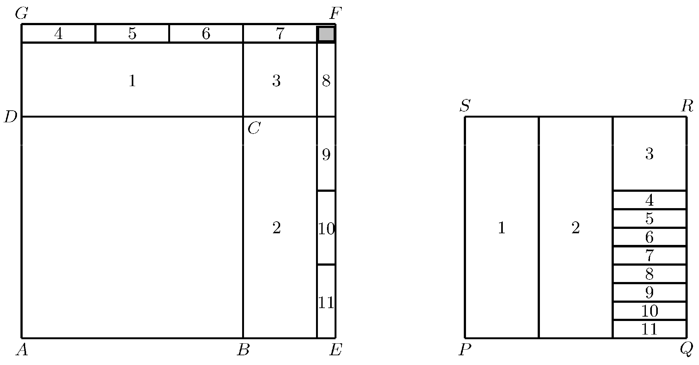
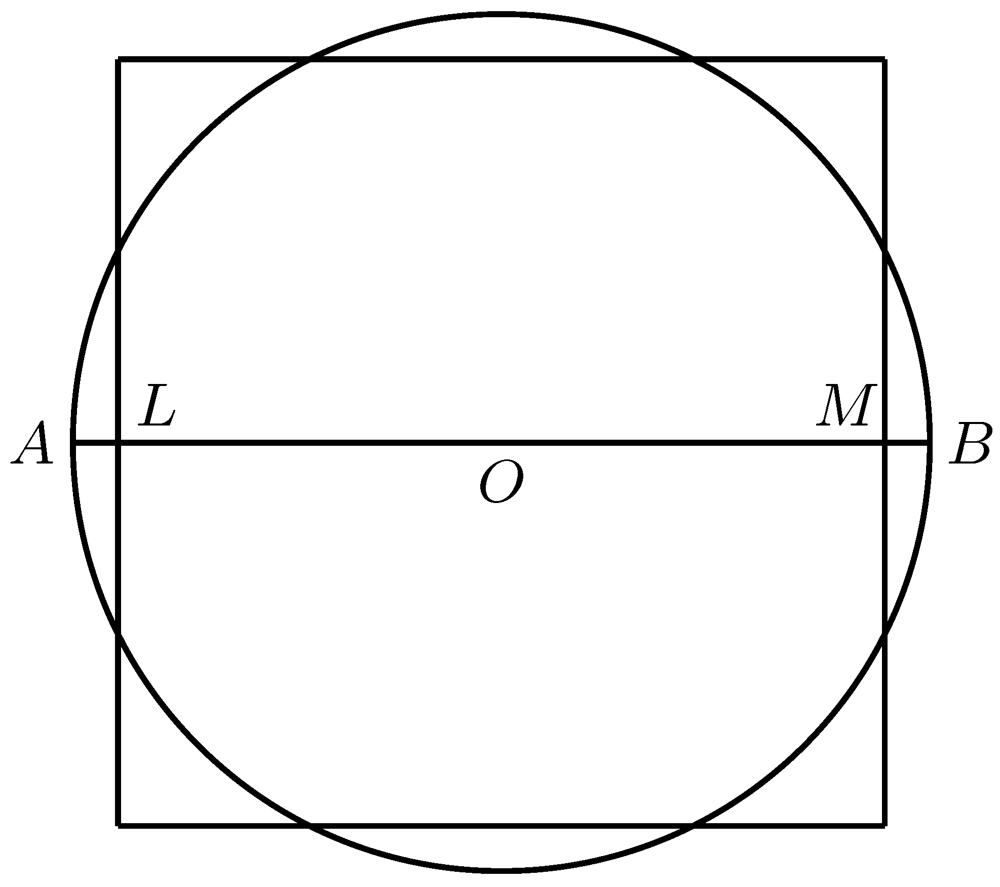
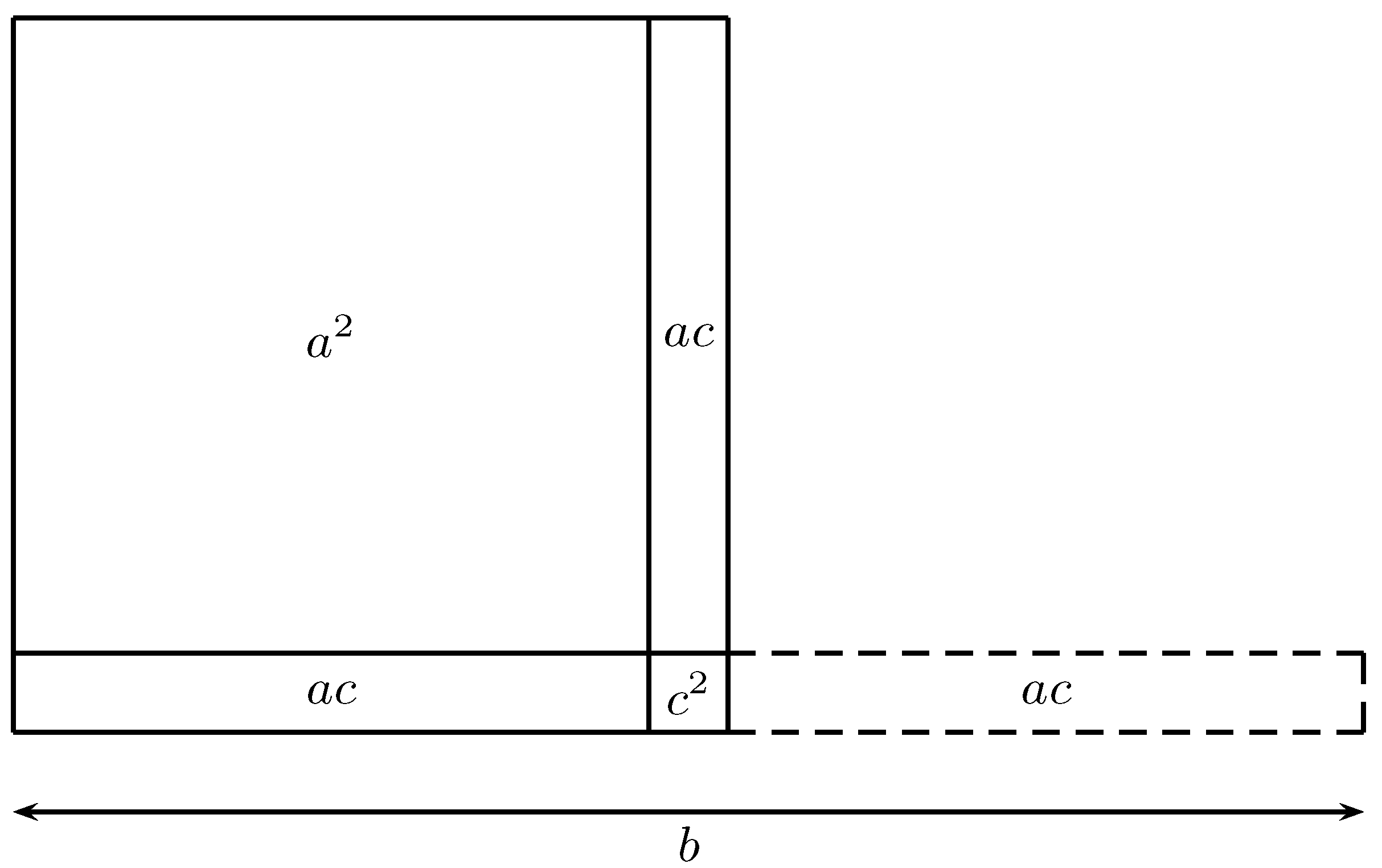
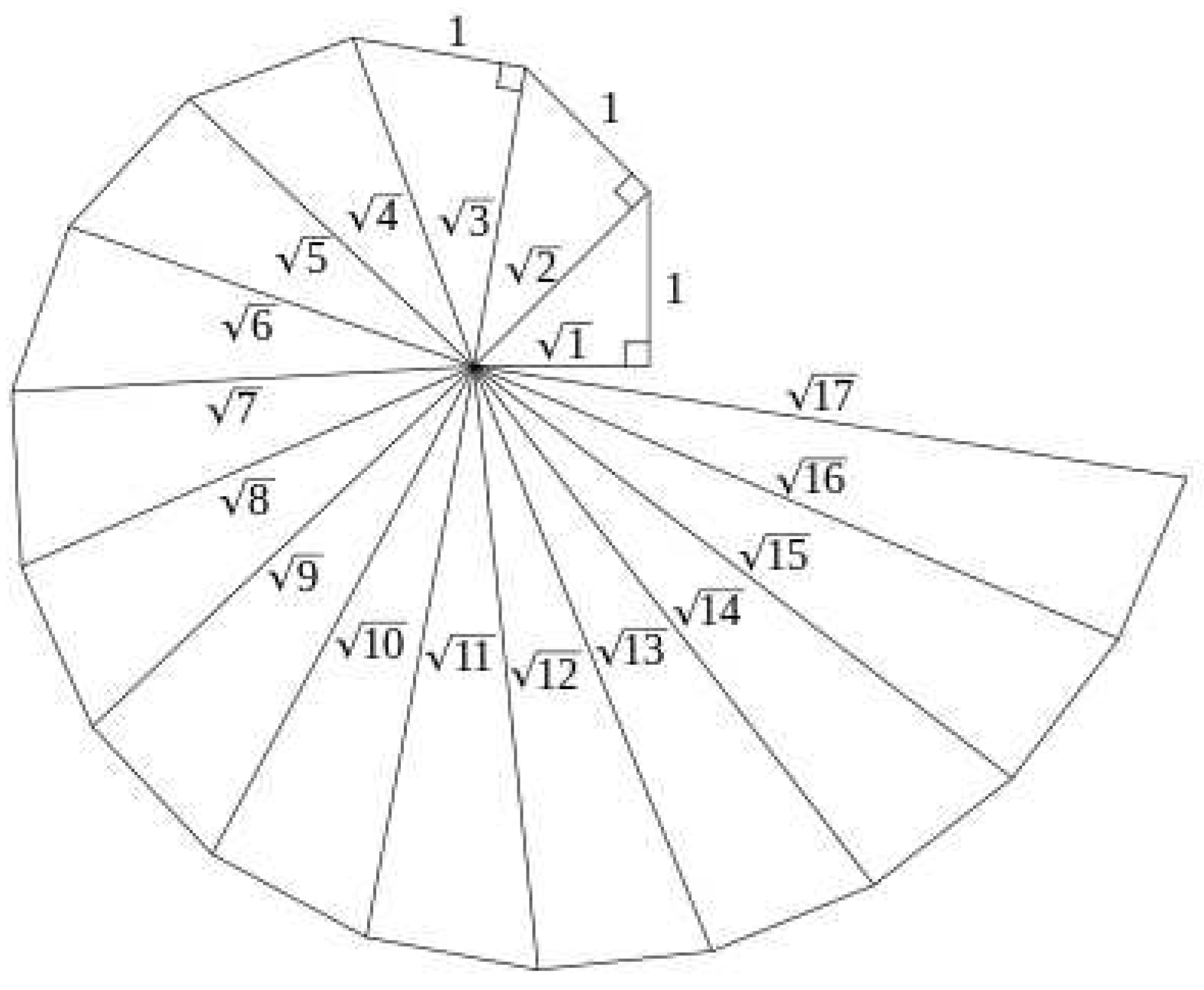
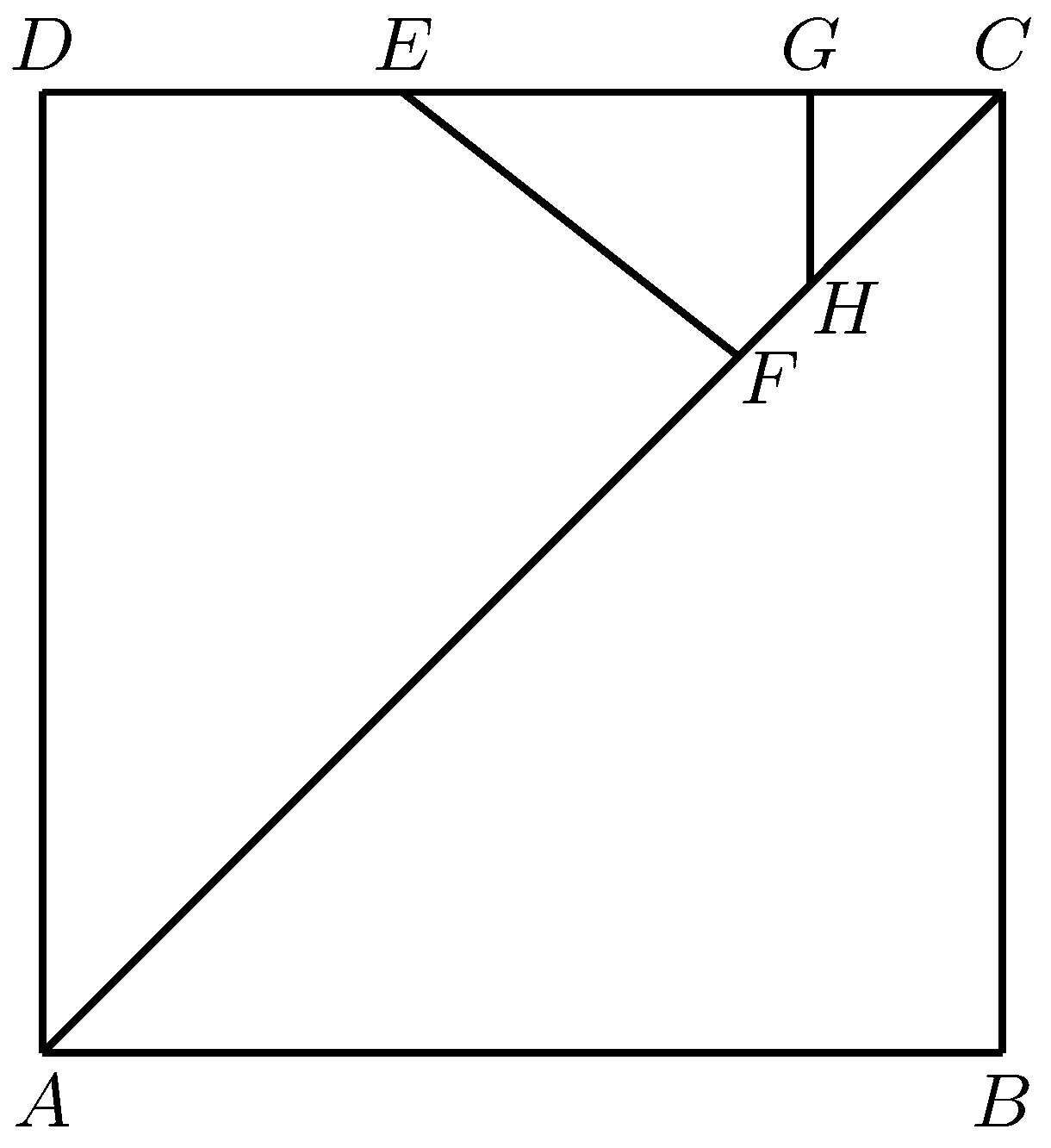
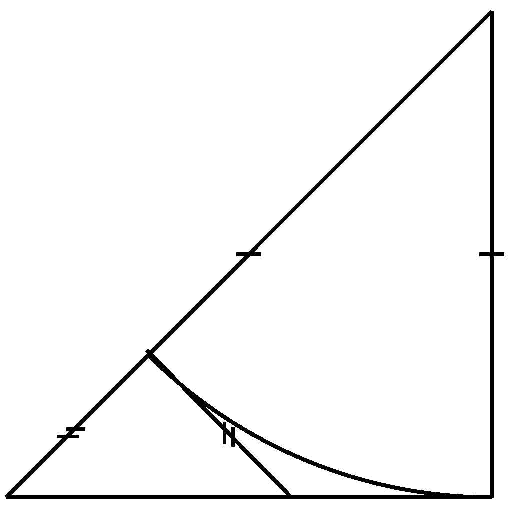
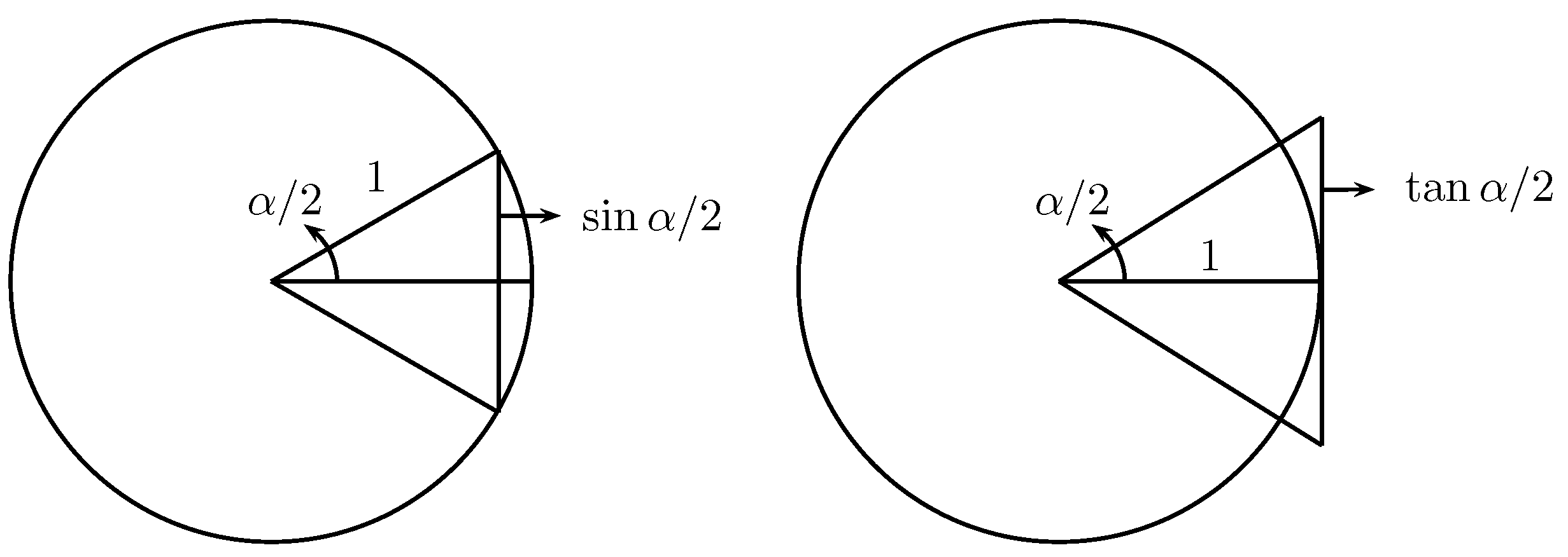
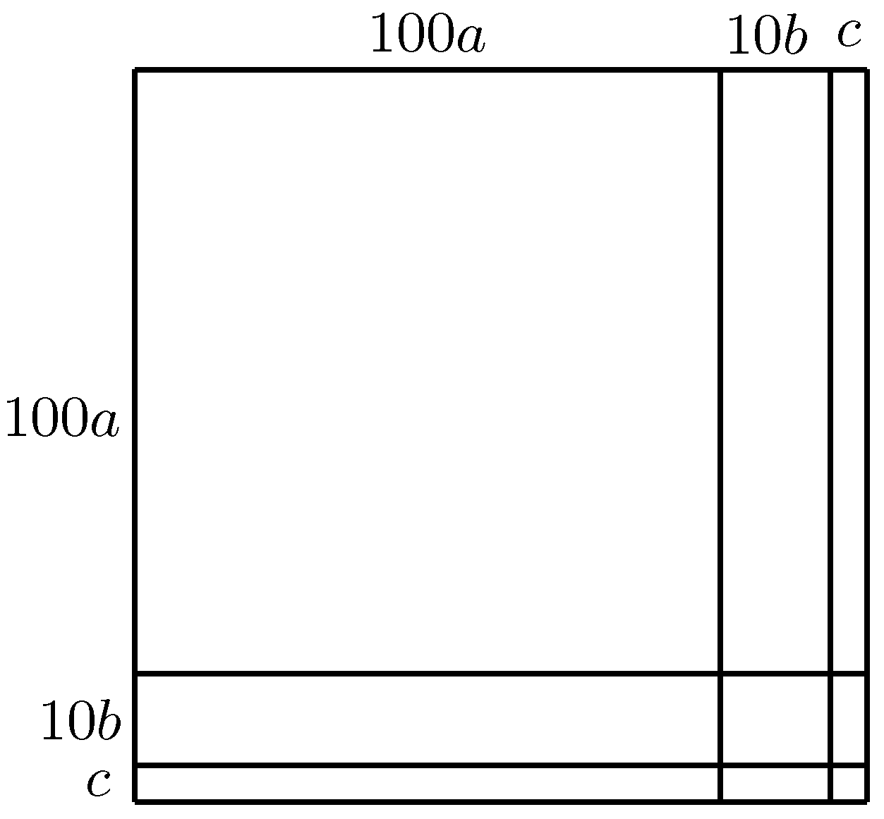
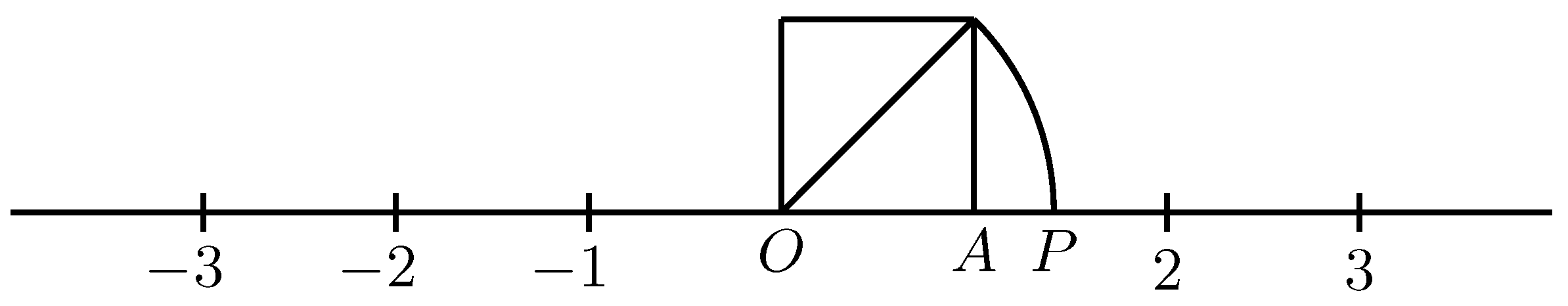
Table 1.
Monotone Convergence.
| n | |||||
|---|---|---|---|---|---|
| 0 | 2 | ||||
| 1 | |||||
| 2 | |||||
| 3 |
Table 2.
Monotone and Oscillatory Convergence.
| Algorithm (25) | Algorithm (26) | |||
|---|---|---|---|---|
| 0 | ||||
| 1 | ||||
| 2 | ||||
| 3 | ||||
Table 3.
Babylonian Ladder Rule.
| N = 2 | N = 3 | |||
|---|---|---|---|---|
| 2 | * | * | ||
| 3 | ||||
| 4 | * | * | ||
| 5 | ||||
| 6 | * | * | ||
| 7 | ||||
| 8 | * | * | ||
| 9 | ||||
| 10 | * | * | ||
| 11 | ||||
| 12 | * | * | ||
| 13 | ||||
| 14 | * | * | ||
| 15 | ||||
| 16 | * | * | ||
Table 4.
Quartic Convergence.
| n | |||||
|---|---|---|---|---|---|
| 0 | |||||
| 1 | |||||
| 2 | |||||
| 0 | |||||
| 1 | |||||
| 2 |
Table 5.
Nonlinear Iterates.
| 0 | ||||
| 1 | ||||
| 2 | ||||
| 3 |
Publisher’s Note: MDPI stays neutral with regard to jurisdictional claims in published maps and institutional affiliations. |
© 2021 by the authors. Licensee MDPI, Basel, Switzerland. This article is an open access article distributed under the terms and conditions of the Creative Commons Attribution (CC BY) license (http://creativecommons.org/licenses/by/4.0/).
Share and Cite
MDPI and ACS Style
Agarwal, R.P.; Agarwal, H. Origin of Irrational Numbers and Their Approximations. Computation 2021, 9, 29. https://0-doi-org.brum.beds.ac.uk/10.3390/computation9030029
AMA Style
Agarwal RP, Agarwal H. Origin of Irrational Numbers and Their Approximations. Computation. 2021; 9(3):29. https://0-doi-org.brum.beds.ac.uk/10.3390/computation9030029
Chicago/Turabian StyleAgarwal, Ravi P., and Hans Agarwal. 2021. "Origin of Irrational Numbers and Their Approximations" Computation 9, no. 3: 29. https://0-doi-org.brum.beds.ac.uk/10.3390/computation9030029
Note that from the first issue of 2016, this journal uses article numbers instead of page numbers. See further details here.