Article

Application of the Generalized Laplace Homotopy Perturbation Method to the Time-Fractional Black–Scholes Equations Based on the Katugampola Fractional Derivative in Caputo Type

by
Sirunya Thanompolkrang
1,
Wannika Sawangtong
1,2 and
Panumart Sawangtong
2,3,*
1
Department of Mathematics, Faculty of Science, Mahidol University, Bangkok 10400, Thailand
2
Center of Excellence in Mathematics, Commission on Higher Education, Bangkok 10400, Thailand
3
Department of Mathematics, Faculty of Applyied Science, King Mongkut’s University of Technology North Bangkok, Bangkok 10800, Thailand
*
Author to whom correspondence should be addressed.
Submission received: 28 January 2021 / Revised: 22 February 2021 / Accepted: 4 March 2021 / Published: 12 March 2021

Abstract

:
In the finance market, the Black–Scholes equation is used to model the price change of the underlying fractal transmission system. Moreover, the fractional differential equations recently are accepted by researchers that fractional differential equations are a powerful tool in studying fractal geometry and fractal dynamics. Fractional differential equations are used in modeling the various important situations or phenomena in the real world such as fluid flow, acoustics, electromagnetic, electrochemistry and material science. There is an important question in finance: “Can the fractional differential equation be applied in the financial market?”. The answer is “Yes”. Due to the self-similar property of the fractional derivative, it can reply to the long-range dependence better than the integer-order derivative. Thus, these advantages are beneficial to manage the fractal structure in the financial market. In this article, the classical Black–Scholes equation with two assets for the European call option is modified by replacing the order of ordinary derivative with the fractional derivative order in the Caputo type Katugampola fractional derivative sense. The analytic solution of time-fractional Black–Scholes European call option pricing equation with two assets is derived by using the generalized Laplace homotopy perturbation method. The used method is the combination of the homotopy perturbation method and generalized Laplace transform. The analytic solution of the time-fractional Black–Scholes equation is carried out in the form of a Mittag–Leffler function. Finally, the effects of the fractional-order in the Caputo type Katugampola fractional derivative to change of a European call option price are shown.

1. Introduction

In 1973, Black and Scholes [1] constructed the mathematical model for pricing an options contract, known as the Black-Scholes model. In particular, the Black-Scholes model estimates the variation over time of financial instruments. The Black-Scholes equation with two assets of a European call option is defined by:
u τ + 1 2 σ 1 2 S 1 2 2 u S 1 2 + 1 2 σ 2 2 S 2 2 2 u 2 S 2 2 + ω σ 1 σ 2 S 1 S 2 2 u S 1 S 2 + r S 1 u S 1 + S 2 u S 2 r u = 0 ,
with the terminal condition:
u ( T , S 1 , S 2 , ) = max β 1 S 1 + β 2 S 2 K , 0 , for S 1 , S 2 [ 0 , ) , τ [ 0 , T ] ,
and boundary conditions:
u ( τ , S 1 , S 2 ) = 0 as ( S 1 , S 2 ) ( 0 , 0 ) ,
and
u ( τ , S 1 , S 2 ) = β 1 S 1 + β 2 S 2 K e r ( T τ ) S 1 or S 2 ,
where
  • u is the call option depending on the underlying asset prices S 1 , S 2 at time τ ,
  • S 1 , S 2 are the asset price variables,
  • σ 1 , σ 2 are the volatility function of underlying assets,
  • β 1 , β 2 are coefficients so that all risky asset price are at the same level,
  • ω is the volatility of S 1 and S 2 ,
  • r is the risk-free interest rate,
  • T is the expiration date,
  • K is strike price of the underlying asset.
During the past 10–20 years, fractional calculus is extensively used for real-life problems in a variety of fields like chemistry, biology, physics, earth science and engineering [2,3,4,5,6,7,8,9,10]. Most of the fractional derivatives are represented in the integral form. Two fractional derivatives, which are the most popular, are Riemann-Liouville derivative [11] and Caputo derivative [12]. Katugampola [13,14] defined a generalized fractional derivative including Riemann-Liouville and Hadamard fractional integrals and derivatives. The Katugampola fractional derivative in Caputo type is defined by Almeida et al. [15] and Jarad et al. [16] that some researchers call this fractional derivative type the Caputo generalized fractional derivative.
The Black-Scholes equation with integer-order derivatives has been developed and studied by many researchers in [17,18,19,20]. Those studies show that the financial market has fractal characters both at home and abroad which is not enough to reflect the reality of the financial market. Recently, fractional differential equations are proved and accepted that fractional differential equations are a powerful tool in studying fractal geometry and fractal dynamics. The concept of the fractional derivative model helps to understand the data structure for the real-life matters deeper than the integer-order derivative model. This is the reason why researchers attempted to develop the integer-order Black-Scholes equation into the fractional-order Black-Scholes equation.
There are many analytical methods, used to find solutions of fractional Black-Scholes equations such as homotopy analysis method, homotopy perturbation method [21], modified homotopy perturbation method [22], Adomain decomposition method [23], analysis of decomposition method [24], finite difference method [25,26,27], variational iteration method with coupling of the Sumudu transform [28], Laplace homotopy perturbation method [29,30,31,32], and ρ -Laplace homotopy perturbation method [33,34].
In 2017, K. Trachoo, W. Sawangtong and P. Sawangtong [32] studied the two dimensional Black-Scholes equation with the integer-order derivative. They used the Laplace homotopy perturbation method to solve the such equation. The analytic solution of this equation is carried out in the form of the special function, which is Mellin-Ross function.
In 2018, P. Sawangtong, K. Trachoo, W. Sawangtong and B. Wiwattanapataphee [31] solved the Black-Scholes equation with two assets in the Liouville-Caputo fractional derivative sense. By the Laplace transform homotopy perturbation method, the analytic solution obtained is in the form of the Generalized Mittag-Leffler function. Moreover, their presented results ensure that the fractional Black-Scholes model is more practical than the integer-order model.
As in previous descriptions, the characteristic of the finance market is fractal geometry and fractal dynamics, and the fractional differential equation is the powerful tool in studying such characteristics. Moreover, the self-similar property of fractional derivative makes can reply to the long-range dependence better than the integer-order derivative. The motivation of this work comes from the two above papers [31,32] and the advantages of fractional calculus. This article studies the fractional-order Black-Scholes equation with two assets described in the sense of the Katugampola Fractional Derivative in Caputo type. We obtain here the analytic solution of the time-fractional Black-Scholes equation with two assets by the technique of the generalized Laplace homotopy perturbation method. Such the method is the combination between homotopy perturbation method and generalized Laplace transform proposed by Jarad and Abdeljawad [35]. Furthermore, the Katugampola fractional derivative in Caputo type can be transformed to both the Caputo derivative and Caputo-Hadamard derivative [36]. In the particular case, analytic solutions of the time-fractional Black-Scholes equation with two assets in the sense of both Caputo derivative and Caputo-Hadamard derivative are shown. We moreover investigate that the fractional-order of the Caputo type Katugampola fractional derivative has an effect on the price of a European call option.
The paper is organized as follows. We introduce the definitions of fractional derivatives, the generalized Laplace transform and the generalized Mittag-Leffler function in Section 2. We recall the constructive partial differential equation associate with the Black-Scholes models in Section 3. In Section 4, the time fractional Black-Scholes equation with two assets of the European call option is determined and carried out by the generalized Laplace homotopy perturbation method. The analytic solutions of fractional Black-Scholes equations and numerical results are presented in Section 5 and Section 6, respectively. Finally, conclusions and a discussion of current work is given in Section 7.

2. Preliminaries

In this section, we give definitions of fractional derivatives and the generalized Laplace transform. Furthermore, some properties of generalized Laplace transform and two-parameters Mittag-Leffler function used throughout this work are shown.
Let α , a , and ρ be any real number with 0 < α 1 , a 0 , ρ > 0 and Γ be a Gamma function.
Definition 1
([37]). The Riemann-Liouville fractional integral of f with order α has the following form:
a I t α f ( t ) = 1 Γ ( α ) a t ( t u ) α 1 f ( u ) d u .
Definition 2
([37]). The Riemann-Liouville fractional derivative of f with order α has the following form:
a D t α f ( t ) = 1 Γ ( 1 α ) d d t a t ( t u ) α f ( u ) d u .
Definition 3
([37]). The Caputo fractional derivative of f with order α has the following form:
a C D t α f ( t ) = 1 Γ ( 1 α ) a t ( t u ) α f ( u ) d u .
Definition 4
([38,39,40]). The Caputo-Hadamard fractional derivative of f with order α has the following form:
a C H D t α f ( t ) = 1 Γ ( 1 α ) a t log t u α δ f ( u ) d u ,
where the differential operator δ is defined by δ = t d d t .
Definition 5
([37]). The Katugampola fractional derivative in Caputo type of f with order α has the following form:
a K C D t α , ρ f ( t ) = 1 Γ ( 1 α ) a t t ρ u ρ ρ α γ f ( u ) d u u 1 ρ ,
where the differential operator γ is given by γ = t 1 ρ d d t .
Note that if ρ = 1 , then the fractional derivative as Equation (4) becomes the Caputo fractional derivative with order α . On the other hand, if ρ approaches 0 , then the fractional derivative as Equation (4) results to the Caputo-Hadamard fractional derivative with order α .
Next, we present the definition of the generalized Laplace transform.
Definition 6
([35]). Let f , g : [ a , ) R be real valued functions such that g ( t ) is continuous and g ( t ) > 0 on [ a , ) . If the generalized Laplace transform of f exists, then
L g f ( t ) ( s ) = a e s ( g ( t ) g ( a ) ) f ( t ) g ( t ) d t ,
where s is the generalized Laplace transform parameter.
Obverse that if we set g ( t ) = t and a = 0 in Equation (5), then the generalized Laplace transform becomes the classical Laplace transform but if we set g ( t ) = t ρ ρ and a = 0 , then the generalized Laplace transform reduces to the ρ - Laplace transform studied by Fall et al. [33].
Throughout this work, we call the generalized Laplace transform with g ( t ) = t ρ ρ and a = 0 by t ρ ρ -Laplace transform. Then, t ρ ρ -Laplace transform is defined by:
L t ρ ρ { f ( t ) } ( s ) = 0 e s t ρ ρ f ( t ) d t t 1 ρ .
We next give some properties of t ρ ρ -Laplace transform.
Lemma 1
([37]).
1. 
L t ρ ρ t ρ ρ ν ( s ) = Γ ( 1 + ν ) s 1 + ν , ν R ,
2. 
L t ρ ρ K C D t α , ρ f ( t ) ( s ) = s α L t ρ ρ { f ( t ) } ( s ) s α 1 f ( 0 ) .
Definition 7
([41,42]). The two-parameters Mittag-Leffler function is defined as follows:
E α , β ( z ) = k = 0 z k Γ ( k α + β ) ,
where α > 0 , β R and z C .
We give some properties of the two-parameters Mittag-Leffler function.
Lemma 2
([43]). The asymptotic expansion of E α , β ( x α ) with α ( 0 , 1 ] and β R is:
E α , β ( x α ) x 1 β e x α as x .
The two-parameters Mittag-Leffler function in Equation (6) and its property in Equation (7) will be used to express the analytic solutions of the fractional-order Black-Scholes equation which described by the Katugampola fractional derivative in Caputo type.

3. Constructive Equations

In this section, we let:
x = ln ( S 1 ) r 1 2 σ 1 2 τ , y = ln ( S 2 ) r 1 2 σ 2 2 τ , t = T τ ,
and
u ( τ , x , y ) = e r ( T τ ) v ( τ , x , y ) .
For more details of transformation, readers can be found in [31,44]. Finally, the Black–Scholes partial differential equation with two assets of the European call option Equation (1) can be transformed in the following form:
v t = 1 2 σ 1 2 2 v x 2 + 1 2 σ 2 2 2 v y 2 + ω σ 1 σ 2 2 v x y , ( t , x , y ) [ 0 , T ] × R × R .
In this work, we consider the Black–Scholes equation in Equation (8) in the general form by replacing the integer-order time derivative with the time-fractional derivative. The time-fractional Black–Scholes equation is studied based on the Katugampola fractional derivative in Caputo type with α ( 0 , 1 ] given by:
K C D t α , ρ v = 1 2 σ 1 2 2 v x 2 + 1 2 σ 2 2 2 v y 2 + ω σ 1 σ 2 2 v x y ,
with the initial condition:
v ( 0 , x , y ; ρ , α ) = max c 1 e x + c 2 e y K , 0 ,
and the boundary conditions:
v ( t , x , y ; ρ , α ) = 0 as ( x , y ) , and
v ( t , x , y ; ρ , α ) = c 1 e x + 1 2 σ 1 2 t + c 2 e y + 1 2 σ 2 2 t K as x or y ,
where c 1 = β 1 e ( r 1 2 σ 1 2 ) T and c 2 = β 2 e ( r 1 2 σ 2 2 ) T .

4. The Generalized Laplace Homotopy Perturbation Method

In this section, we present the basic idea of the generalized Laplace homotopy perturbation method with g ( t ) = t ρ ρ and a = 0 for the time-fractional differential equations.
Firstly, we consider the following problem:
K C D t α , ρ u ( t , x , y ; ρ , α ) + R u ( t , x , y ; ρ , α ) + N u ( t , x , y ; ρ , α ) = f ( t , x , y ) for ( t , x , y ) ( 0 , T ] × R × R ,
with the initial condition:
u ( 0 , x , y ; ρ , α ) = h ( x , y ) for any ( x , y ) R × R ,
where R and N are the linear and nonlinear operators and f and h are determined functions.
Step 1. By taking the generalized Laplace transform with respect to time variable t in Equation (12), we obtain:
L t ρ ρ { K C D t α , ρ u ( t , x , y ; ρ , α ) } ( s ) + L t ρ ρ { R ( u ( t , x , y ; ρ , α ) ) + N ( u ( t , x , y ; ρ , α ) ) } ( s ) = L t ρ ρ { f ( t , x , y ) } ( s ) .
Step 2. By using the generalized Laplace transform of Katugampola fractional derivative in Caputo type, we have:
L t ρ ρ { u } ( s ) = s 1 h ( x , y ) s α L t ρ ρ { R ( u ) + N ( u ) } ( s ) + s α L t ρ ρ { f ( t , x , y ) } ( s ) .
Step 3. By taking the inverse generalized Laplace transform on the both sides in Equation (14), we get:
u ( t , x , y ; ρ , α ) = G ( t , x , y ) L t ρ ρ 1 { s α L t ρ ρ { R ( u ) + N ( u ) } ( s ) } ( t ) ,
where
G ( t , x , y ) = L t ρ ρ 1 s 1 h ( x , y ) + s α L t ρ ρ { f ( t , x , y ) } ( t ) .
Step 4. By applying the homotopy perturbation technique [45,46], the homotopy function ν ( t , x , y ; p ) is defined by the homotopy equation:
ν ( t , x , y ; p ) = ν ˜ 0 ( t , x , y ) p ν ˜ 0 ( t , x , y ) G ( t , x , y ) + L t ρ ρ 1 { s α L t ρ ρ { R ( ν ( t , x , y ; p ) ) + N ( ν ( t , x , y ; p ) ) } }
where p [ 0 , 1 ] denote homotopy parameter and ν ˜ 0 ( t , x , y ) is an arbitrary initial approximation satisfying both the initial and boundary conditions of the problem [47].
Note that we can see that when p = 1 in Equation (15), the homotopy function ν ( t , x , y ; 1 ) is the solution of the problem Equation (12). We assume that:
ν ( t , x , y ; p ) = n = 0 p n ν n ( t , x , y )
and the nonlinear term can be applied as:
N ν ( t , x , y ; p ) = n = 0 p n H n ( ν 0 , ν 1 , , ν n ) .
The He’s polynomials H n ( ν 0 , ν 1 , , ν n ) can be calculated by using the following formula:
H n ( ν 0 , ν 1 , ν 2 , , ν n ) = 1 n ! n p n N i = 0 n p i ν i | p = 0 , n = 0 , 1 , 2 , .
Step 5. By substituting Equations (16) and (17) into (15), we obtain:
n = 0 p n ν n ( t , x , y ) = ν ˜ 0 ( t , x , y ) p [ ν ˜ 0 ( t , x , y ) G ( t , x , y ) + L t ρ ρ 1 { s α L t ρ ρ { R ( n = 0 p n ν n ( t , x , y ) ) + n = 0 p n H n ( ν 0 , ν 1 , , ν n ) } ( s ) } ( t ) ] .
Step 6. By comparing the coefficient of like power of p on both sides of Equation (18), the sequence ν n is carried out:
p 0 : ν 0 ( t , x , y ) = ν ˜ 0 ( t , x , y ) , p 1 : ν 1 ( t , x , y ) = G ( t , x , y ) ν ˜ 0 ( t , x , y ) L t ρ ρ 1 { s α L t ρ ρ { R ( ν ˜ 0 ( t , x , y ) ) + H 0 ( t , x , y ) ) } ( s ) } ( t ) , p n : ν n ( t , x , y ) = L t ρ ρ 1 { s α L t ρ ρ { R ( ν n 1 ( t , x , y ) ) + H n 1 ( t , x , y ) ) } ( s ) } ( t ) when n 2 .
Step 7. The approximate analytic solution of problem Equations (12) and (13) can be expressed in the following form:
u ( t , x , y ; ρ , α ) = ν ( t , x , y ; 1 ) = n = 0 ν n ( t , x , y ) .

5. Analytic Solutions for the Time-Fractional Black–Scholes Equation

In this section, we solve the time-fractional Black–Scholes equation Equation (9) subjecting to the initial condition Equation (10) and the boundary conditions Equation (11) by the generalized Laplace homotopy perturbation method.
From Equations (9) and (12), we can see that:
R ( v ( t , x , y ; ρ , α ) ) = 1 2 σ 1 2 2 v x 2 + 1 2 σ 2 2 2 v y 2 + ω σ 1 σ 2 2 v x y ,
and N v ( t , x , y ; ρ , α ) = 0 , f ( t , x , y ) = 0 , with the initial condition as:
v ( 0 , x , y ; ρ , α ) = h ( x , y ) = max ( c 1 e x + c 2 e y K , 0 ) .
Note that since the nonlinear term is zero, the He’s polynomials H n = 0 for all n = 1 , 2 , 3 , .
From the recurrence relation Equation (19), we choose the function v ˜ 0 by:
v ˜ 0 ( t , x , y ) = max ( c 1 e x + c 2 e y K , 0 ) .
We next find the function v 1 by using Equation (19). Then,
v 1 ( t , x , y ) = G ( t , x , y ) v ˜ 0 ( t , x , y ) L t ρ ρ 1 { s α L t ρ ρ { R ( v ˜ 0 ( t , x , y ) ) + H 0 ( t , x , y ) ) } ( s ) } ( t ) = L t ρ ρ 1 1 s α L t ρ ρ 1 2 σ 1 2 2 v 0 x 2 + 1 2 σ 2 2 2 v 0 y 2 + ω σ 1 σ 2 2 v 0 x y ( s ) ( t ) = L t ρ ρ 1 1 s α + 1 1 2 σ 1 2 max ( c 1 e x , 0 ) + 1 2 σ 2 2 max ( c 2 e y , 0 ) ( t ) = 1 2 σ 1 2 max ( c 1 e x , 0 ) + 1 2 σ 2 2 max ( c 2 e y , 0 ) 1 Γ ( 1 + α ) t ρ ρ α .
Therefore,
v 1 ( t , x , y ) = 1 2 σ 1 2 max ( c 1 e x , 0 ) + 1 2 σ 2 2 max ( c 2 e y , 0 ) 1 Γ ( 1 + α ) t ρ ρ α .
By Equation (19), we obtain that:
v 2 ( t , x , y ) = L t ρ ρ 1 { s α L t ρ ρ { R ( v 1 ( t , x , y ) ) + H 1 ( t , x , y ) ) } ( s ) } ( t ) = L t ρ ρ 1 1 s α L t ρ ρ 1 2 σ 1 2 2 v 1 x 2 + 1 2 σ 2 2 2 v 1 y 2 + ω σ 1 σ 2 2 v 1 x y ( t ) = 1 2 2 σ 1 4 max ( c 1 e x , 0 ) + 1 2 2 σ 2 4 max ( c 2 e y , 0 ) 1 Γ ( 1 + 2 α ) t ρ ρ 2 α .
Hence,
v 2 ( t , x , y ) = 1 2 2 σ 1 4 max ( c 1 e x , 0 ) + 1 2 2 σ 2 4 max ( c 2 e y , 0 ) 1 Γ ( 1 + 2 α ) t ρ ρ 2 α .
It follows from Equation (19) that:
v 3 ( t , x , y ) = L t ρ ρ 1 1 s α L t ρ ρ 1 2 σ 1 2 2 v 2 x 2 + 1 2 σ 2 2 2 v 2 y 2 + ω σ 1 σ 2 2 v 2 x y ( s ) ( t ) = 1 2 3 σ 1 6 max ( c 1 e x , 0 ) + 1 2 3 σ 2 6 max ( c 2 e y , 0 ) 1 Γ ( 1 + 3 α ) t ρ ρ 3 α .
Then,
v 3 ( t , x , y ) = 1 2 3 σ 1 6 max ( c 1 e x , 0 ) + 1 2 3 σ 2 6 max ( c 2 e y , 0 ) 1 Γ ( 1 + 3 α ) t ρ ρ 3 α .
Like the same manner, we can conclude that by Equation (19),
v n ( t , x , y ) = L t ρ ρ 1 1 s α L t ρ ρ 1 2 σ 1 2 2 v n 1 x 2 + 1 2 σ 2 2 2 v n 1 y 2 + ω σ 1 σ 2 2 v n 1 x y ( s ) ( t ) = 1 2 n σ 1 2 n max ( c 1 e x , 0 ) + 1 2 n σ 2 2 n max ( c 2 e y , 0 ) 1 Γ ( 1 + n α ) t ρ ρ n α .
for n = 1 , 2 , 3 , . Therefore, by Equation (15), the homotopy perturbation v ( t , x , y ; p ) which corresponds to problem Equations (12) and (13) is in the form:
v ( t , x , y ; p ) = max c 1 e x + c 2 e y K , 0 + n = 0 p n + 1 1 Γ ( 1 + ( n + 1 ) α ) t ρ ρ ( n + 1 ) α 1 2 ( n + 1 ) σ 1 2 ( n + 1 ) max c 1 e x , 0 + n = 0 p n + 1 1 Γ ( 1 + ( n + 1 ) α ) t ρ ρ ( n + 1 ) α 1 2 ( n + 1 ) σ 2 2 ( n + 1 ) max c 2 e y , 0 .
By Equation (20), we obtain the analytic solution of problem Equations (9)–(11) defined by:
v ( t , x , y ; ρ , α ) = v ( t , x , y ; 1 ) = max c 1 e x + c 2 e y K , 0 + n = 0 1 Γ ( 1 + ( n + 1 ) α ) t ρ ρ ( n + 1 ) α 1 2 ( n + 1 ) σ 1 2 ( n + 1 ) max c 1 e x , 0 + n = 0 1 Γ ( 1 + ( n + 1 ) α ) t ρ ρ ( n + 1 ) α 1 2 ( n + 1 ) σ 2 2 ( n + 1 ) max c 2 e y , 0 = max c 1 e x + c 2 e y K , 0 + σ 1 2 2 t ρ ρ α max ( c 1 e x , 0 ) n = 0 1 Γ ( α + 1 + n α ) σ 1 2 2 t ρ ρ α n + σ 2 2 2 t ρ ρ α max ( c 2 e y , 0 ) n = 0 1 Γ ( α + 1 + n α ) σ 2 2 2 t ρ ρ α n ,
or
v ( t , x , y ; ρ , α ) = max c 1 e x + c 2 e y K , 0 + σ 1 2 2 t ρ ρ α max c 1 e x , 0 E α , α + 1 σ 1 2 2 t ρ ρ α + σ 2 2 2 t ρ ρ α max c 2 e y , 0 E α , α + 1 σ 2 2 2 t ρ ρ α ,
where E α , α + 1 is the two-parameters Mittag–Leffler function defined by Equation (6).
Hence, the analytic solution of the time fractional Black-Scholes equations in the sense of Caputo type Katugampola fractional derivative Equations (9)–(11) is given by Equation (21).
It follows from [36] that as ρ = 1 , the time-fractional Black–Scholes equation with two assets for the European call option based on Caputo type Katugampola fractional derivative becomes the time-fractional Black–Scholes equation with two assets for the European call option based on Caputo fractional derivative:
C D t α v = 1 2 σ 1 2 2 v x 2 + 1 2 σ 2 2 2 v y 2 + ω σ 1 σ 2 2 v x y ,
with the initial condition:
v ( 0 , x , y ; 1 , α ) = max ( c 1 e x + c 2 e y K , 0 ) ,
and the boundary conditions:
v ( t , x , y ; 1 , α ) = 0 as ( x , y ) , and
v ( t , x , y ; 1 , α ) = c 1 e x + 1 2 σ 1 2 t + c 2 e y + 1 2 σ 2 2 t K as x or y ,
where c 1 and c 2 are constants.
By (21), the analytic solution of the time-fractional Black–Scholes equation with two assets for the European call option in Caputo fractional derivative sense is defined:
v ( t , x , y ; 1 , α ) = max c 1 e x + c 2 e y K , 0 + σ 1 2 t α 2 max c 1 e x , 0 E α , α + 1 σ 1 2 t α 2 + σ 2 2 t α 2 max c 2 e y , 0 E α , α + 1 σ 2 2 t α 2 ,
which differs from the solution studied in [31]. The reason is why we obtain another solution because choosing the initial function ν ˜ 0 ( t , x , y ) in recurrence relation (19) is different. In the particular case, if we let ρ = 1 and α = 1 , then the time-fractional Black–Scholes equation reduces to the classical Black–Scholes equation with two assets as Equation (8). It follows from the property of Mittag–Leffler function with two parpmeters, that is E 1 , 2 ( z ) = e z 1 z , that the analytic solution of the classical Black–Scholes equation with two assets for the European call option is given by:
v ( t , x , y ; 1 , 1 ) = max c 1 e x + c 2 e y K , 0 + σ 1 2 t 2 max c 1 e x , 0 E 1 , 2 σ 1 2 t 2 + σ 2 2 t 2 max c 2 e y , 0 E 1 , 2 σ 2 2 t 2 = max c 1 e x + c 2 e y K , 0 + max c 1 e x , 0 e σ 1 2 t 2 1 + max c 2 e y , 0 e σ 2 2 t 2 1 ,
which differs from the solution obtained by [32] because choosing the initial function ν ˜ 0 ( t , x , y ) in recurrence relation (19) is different.
We next consider the case when ρ approaches to 0 + .
More precisely, as ρ approaches to 0 + , the time-fractional Black-Scholes equation with two assets for the European call option based on Caputo type Katugampola fractional derivative Equations (9)–(11) becomes the time-fractional Black-Scholes equation with two assets for the European call option in sense of the Caputo-Hadamard fractional derivative.
Consider the terms E α , α + 1 σ i 2 2 1 α t ρ ρ α for i = 1 and 2 .
By using the property in Lemma 2 as Equation (7) we have that for each i = 1 and 2 ,
E α , α + 1 σ i 2 2 1 α t ρ ρ α 1 α σ i 2 2 1 α t ρ ρ α e σ i 2 2 1 α t ρ ρ as ρ 0 + .
It follows from Equation (21) that the analytic solution of the time-fractional Black–Scholes equation in the Caputo–Hadamard fractional derivative is in the form:
lim ρ 0 + v ( t , x , y ; ρ , α ) = max c 1 e x + c 2 e y K , 0 + lim ρ 0 + σ 1 2 2 t ρ ρ α max c 1 e x , 0 E α , α + 1 σ 1 2 2 t ρ ρ α + lim ρ 0 + σ 2 2 2 t ρ ρ α max c 2 e y , 0 E α , α + 1 σ 2 2 2 t ρ ρ α = max c 1 e x + c 2 e y K , 0 + 1 α max c 1 e x , 0 e σ 1 2 2 1 α t ρ ρ + 1 α max c 2 e y , 0 e σ 2 2 2 1 α t ρ ρ .
We see that lim ρ 0 + v ( t , x , y ; ρ , α ) for all ( t , x , y ) [ 0 , T ] × R × R . This means that lim ρ 0 + v ( t , x , y ; ρ , α ) is unbounded for any ( t , x , y ) [ 0 , T ] × R × R which contradicts to the initial condition: v ( 0 , x , y ; ρ , α ) = max c 1 e x + c 2 e y K , 0 . This implies that the time-fractional Black–Scholes equation with two assets in Caputo–Hadamard sense has no solution.

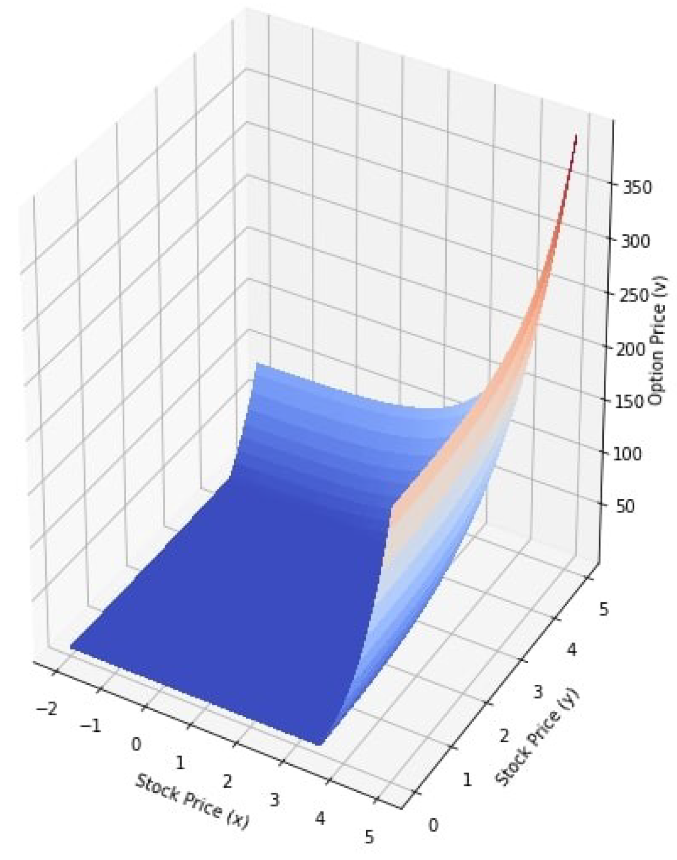
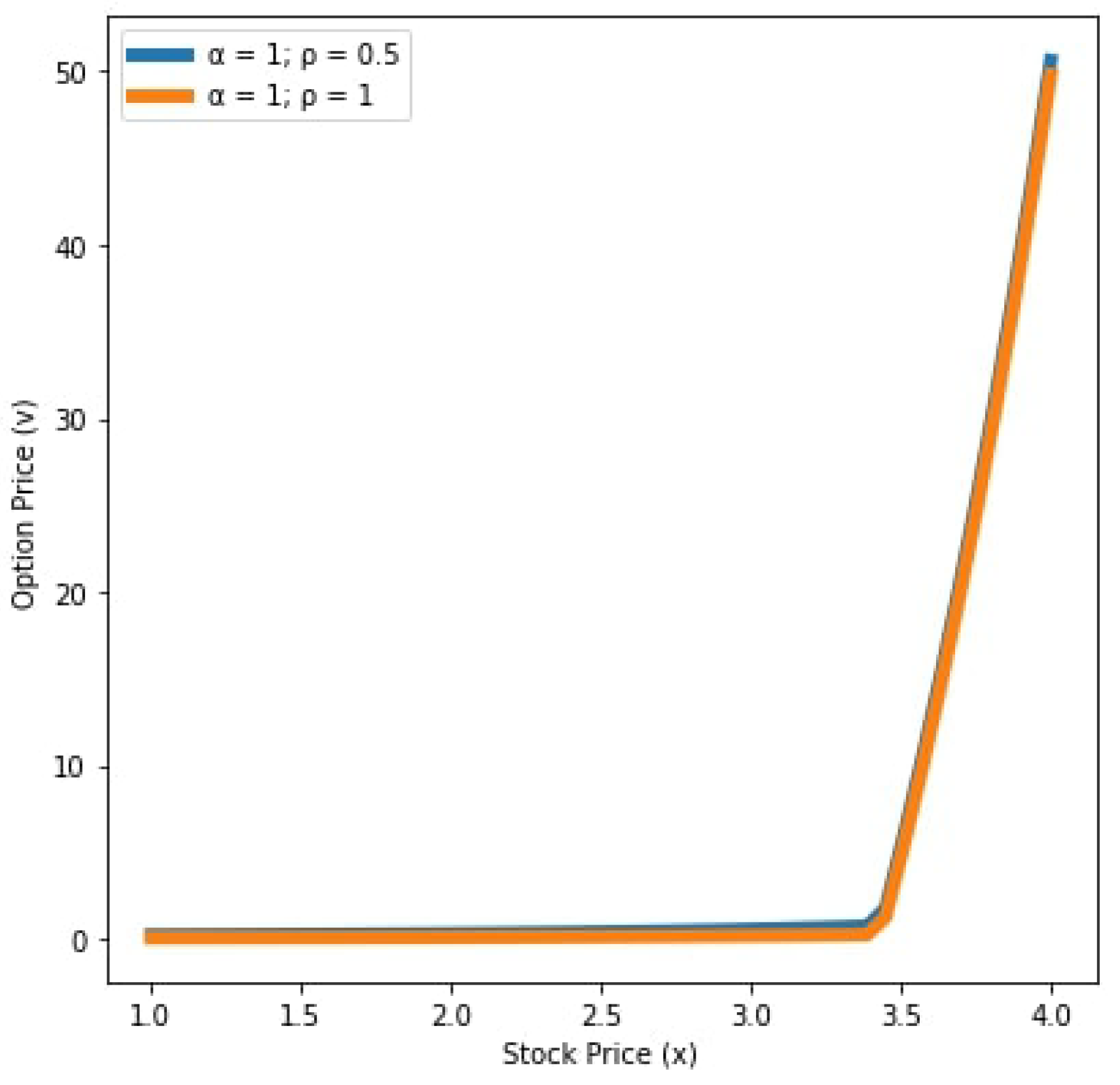
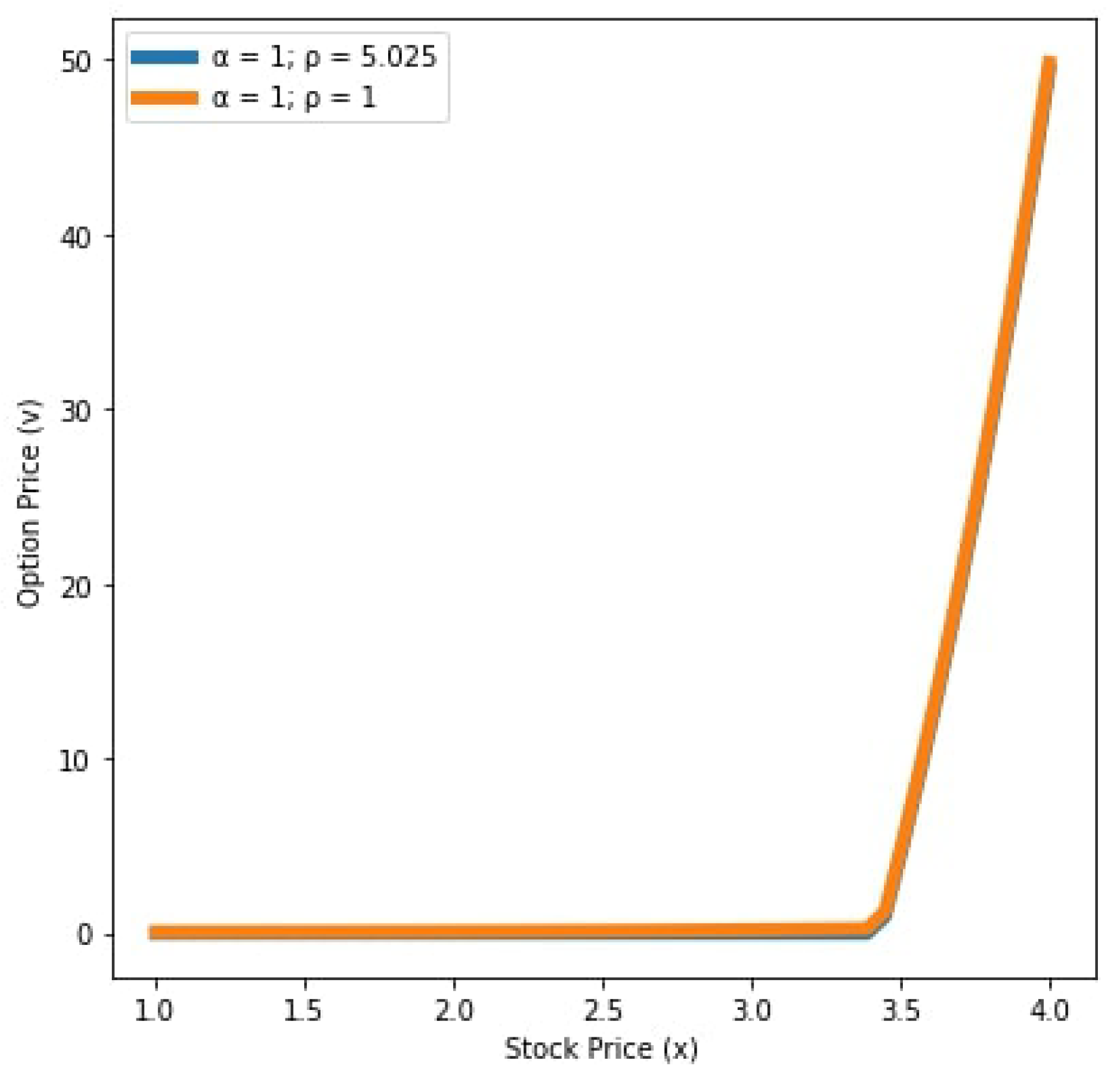
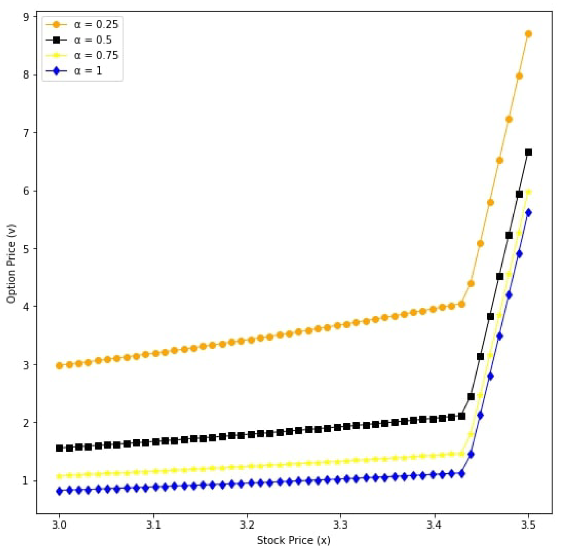
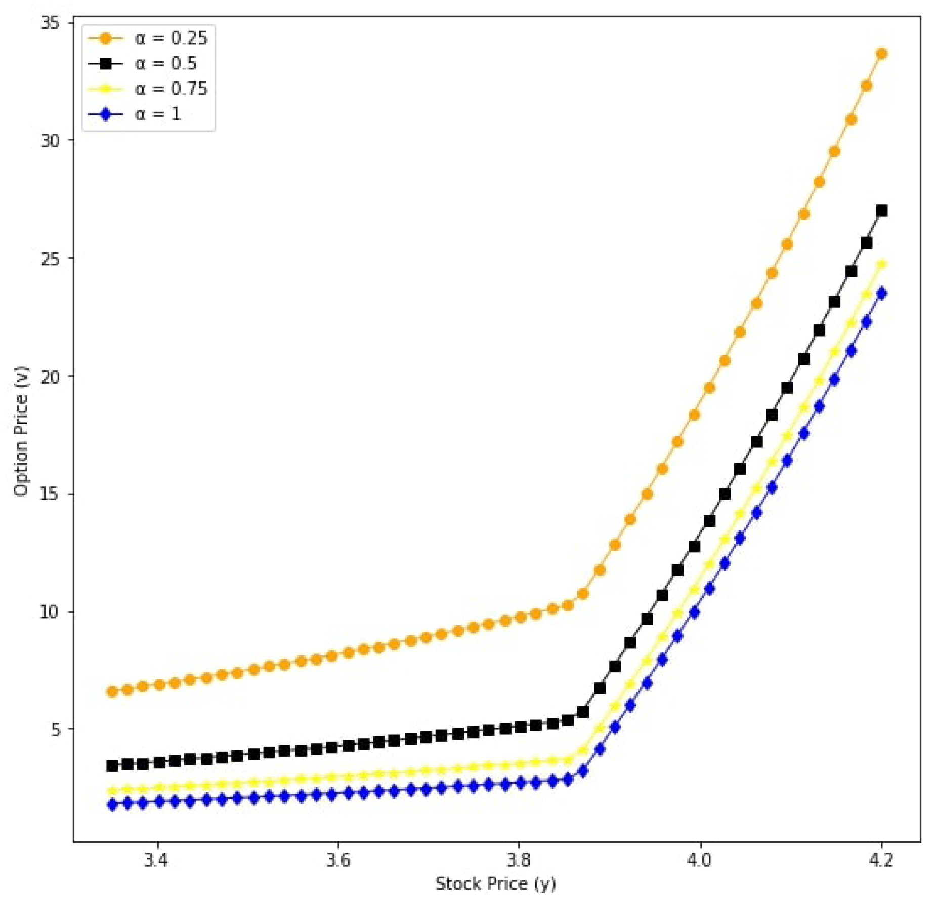
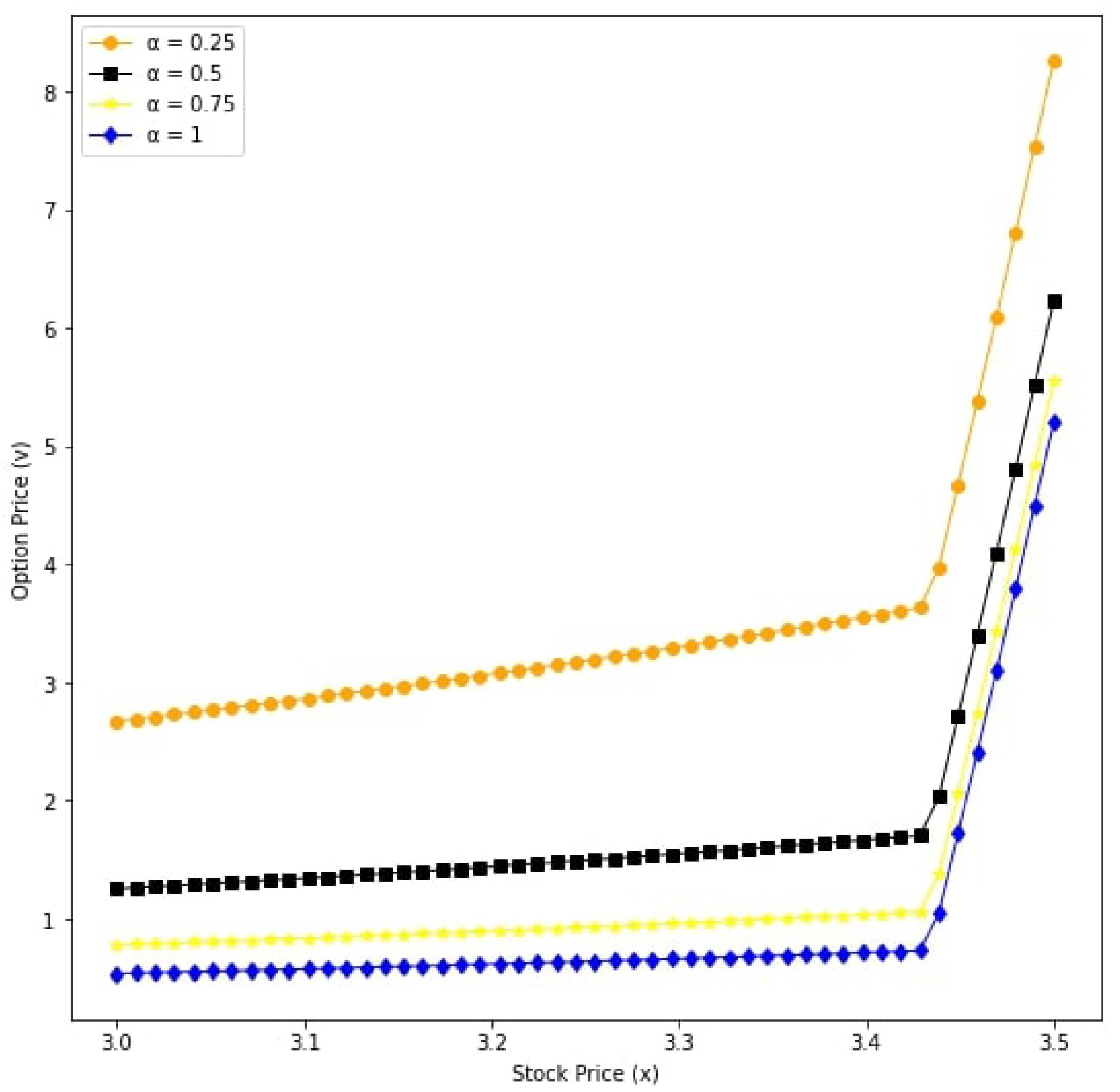
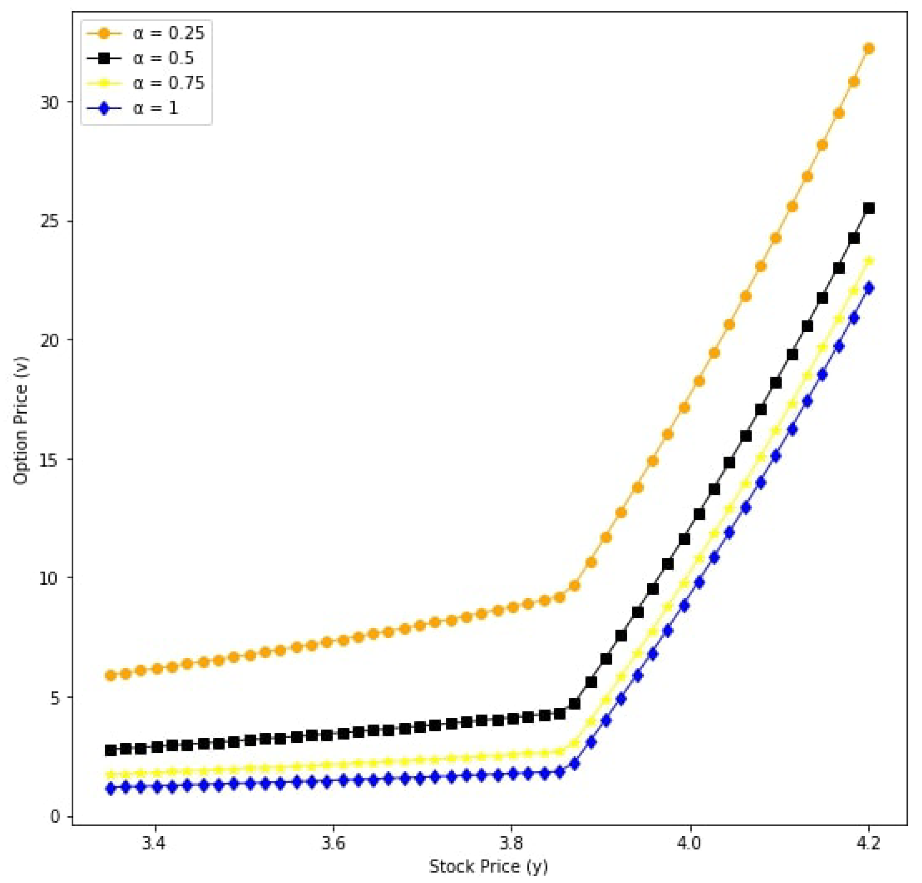
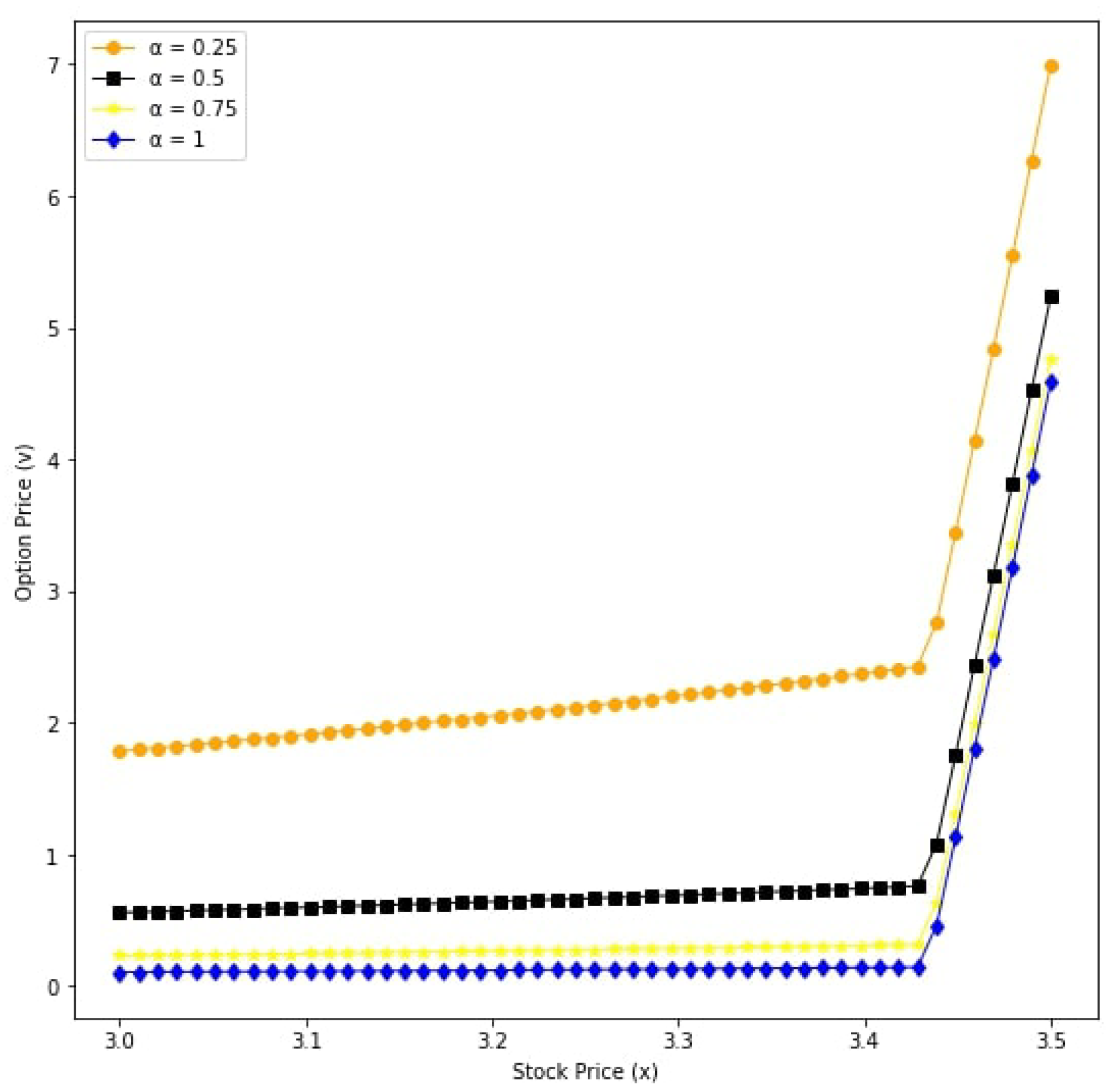
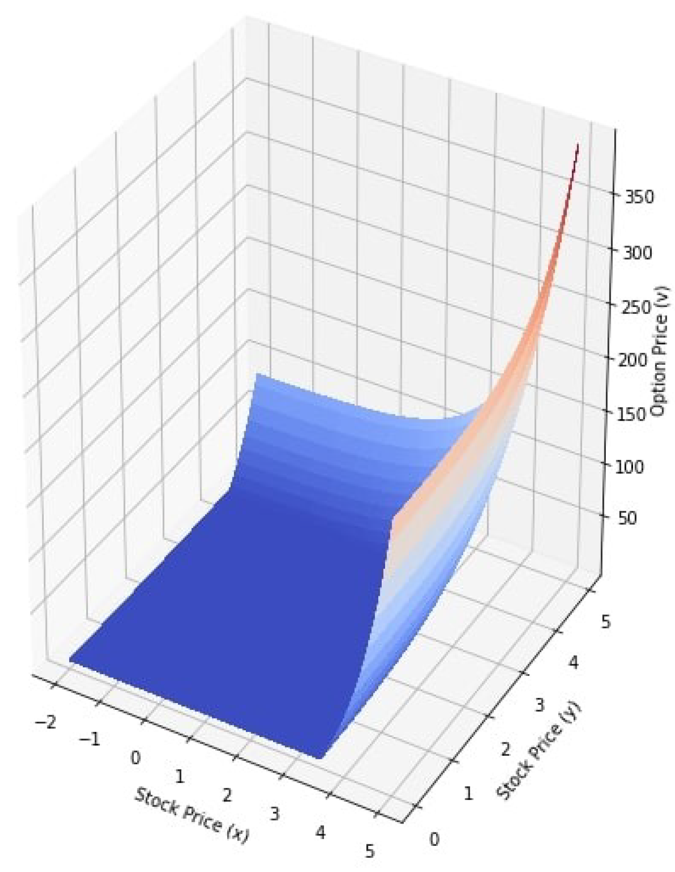
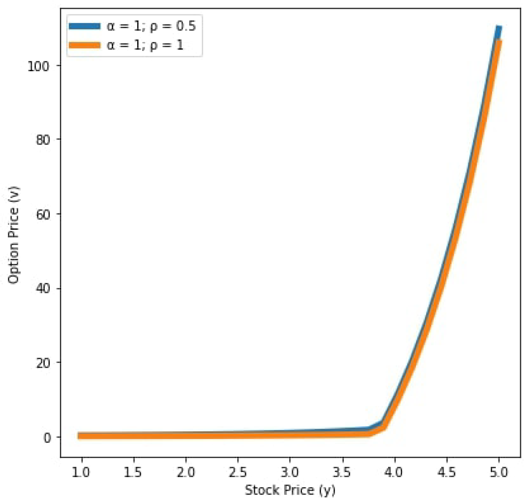
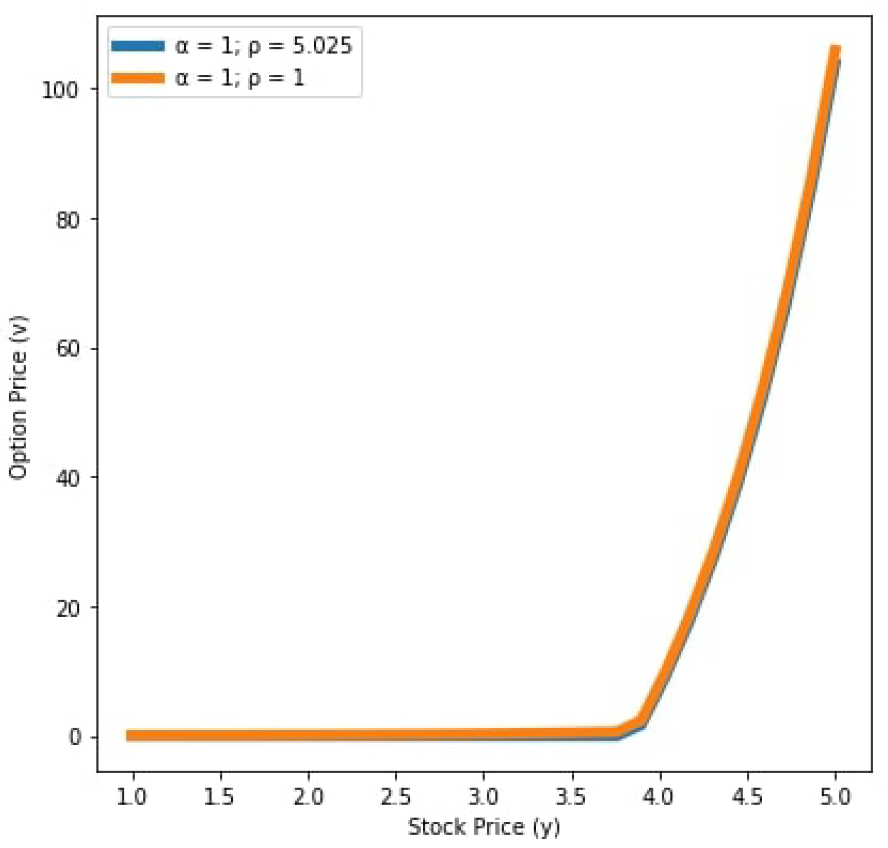
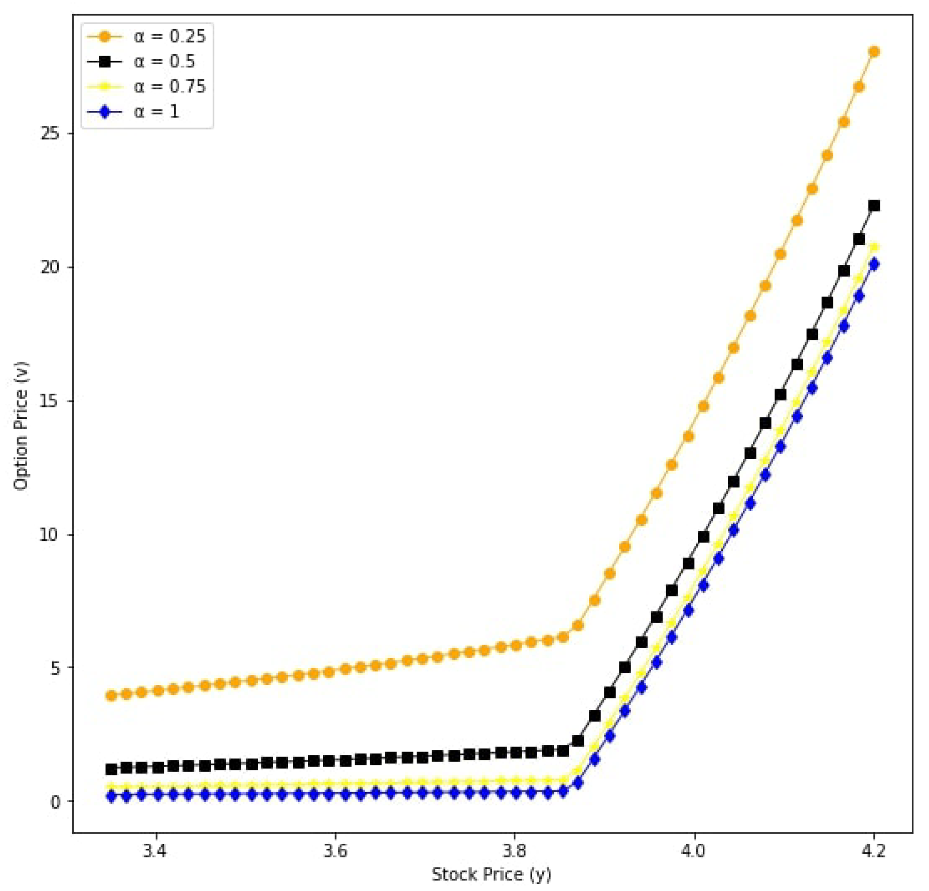
6. Numerical Results

In this section, we illustrate the analytic solution of the time-fractional Black–Scholes equation with two assets for European call option based on Caputo type Katugampola fractional derivative by using Python programming. The financial parameters are given in Table 1.
The classical values of the options ( α = ρ = 1 ) defined by (22) are simulated in Figure 1. In Figure 2, Figure 3 and Figure 4, we have depicted the values of the options in Equation (21) for α = 1 and ρ = 0.85 , α = 0.75 and ρ = 1 , and α = 1 and ρ = 1.15 , respectively. We note that the analytic solution of the time-fractional Black-Scholes equation described in the sense of Caputo type Katugampola fractional derivative and the analytic solution of the classical Black-Scholes equation with both of the two assets are in good agreement. The European call option prices for different values of α and ρ are shown in Table 2.
We see that in Figure 5 and Figure 6, the values of x and y in the case ρ < 1 are greater than the values of x and y in the case ρ = 1 . This means that the order ρ of the Caputo type Katugampola fractional derivative has an acceleration effect in the diffusion process when ρ < 1 . On the other hand, in Figure 7 and Figure 8, the values of x and y in the case ρ > 1 are less than the values of x and y in the case ρ = 1 . This implies that the order ρ of the Caputo type Katugampola fractional derivative has a retardation effect in the diffusion process when ρ > 1 .
From the Figure 9, Figure 10, Figure 11, Figure 12, Figure 13 and Figure 14, we see that the payoff of the European option increases as α decreases. Moreover, we observe that the European option price is overpriced when α = 0.25 .

7. Conclusions

In this paper, we have discussed the analytic solution of the time-fractional Black–Scholes equation with two assets in sense of the Katugampola fractional derivative in Caputo type. The method, used here to provide analytical solutions, is called the generalized Laplace homotopy perturbation method. The idea of the generalized Laplace homotopy perturbation method comes from combining the technique of both the homotopy perturbation method and generalized Laplace transform. The result in Equation (21) shows that the analytic solution of the time-fractional Black–Scholes equations in the sense of Caputo type Katugampola fractional derivative can be carried out in the form of the two-parameters Mittag–Leffler function. Since the Katugampola fractional derivative in Caputo type generalizes both Caputo and Caputo–Hadamard derivatives, in the case of the time-fractional Black–Scholes equations in the Caputo derivative sense, the analytic solution is also obtained. Unfortunately, in the case of the time-fractional Black–Scholes equations in the Caputo-Hadamard derivative sense, there is no solution. Moreover, we can observe that the orders ρ and α of the Katugampola fractional derivative in Caputo type have an effect on the price of the European option. Moreover, the European option price is overpriced when α = 0.25 .

Author Contributions

Conceptualization, P.S.; methodology, P.S. and S.T.; validation, P.S. and S.T.; formal analysis, S.T., W.S. and P.S.; writing—original draft preparation, S.T.; writing—review and editing, W.S. and P.S.; supervision, P.S.; project administration, P.S.; funding acquisition, P.S. All authors have read and agreed to the published version of the manuscript.

Funding

This research was funded by King Mongkut’s University of Technology North Bangkok, 133 contract no. KMUTNB-FF-65-58 and this research was partially supported by the Centre of Excellence in 134 Mathematics, PERDO, Commission on Higher Education, Ministry of Education, Thailand.

Institutional Review Board Statement

Not applicable.

Informed Consent Statement

Not applicable.

Data Availability Statement

The information used to support the findings of this study are available in the article, in the links there provided or from the corresponding author upon request.

Conflicts of Interest

The authors declare no conflict of interest.

References

  1. Black, F.; Scholes, M. The pricing of options and corporate liabilities. J. Political Econ. 1973, 81, 637–654. [Google Scholar] [CrossRef] [Green Version]
  2. Atangana, A.; Baleanu, D.; Alsaedi, A. Analysis of time-fractional Hunter-Saxton equation: A model of neumatic liquid crystal. Open Phys. 2016, 14, 145–149. [Google Scholar] [CrossRef]
  3. Hristov, T. A transient flow of a non-newtonian fluid modelled by a mixed time-space derivative: An improved integral-balance approach. In Mathematical Methods in Engineering; Springer: Cham, Switzerland, 2019; pp. 153–174. [Google Scholar]
  4. Mainardi, F. Fractional relaxation-oscillation and fractional diffusion-wave phenomena. Chaos Solitons Fractals 1996, 9, 1461–1477. [Google Scholar] [CrossRef]
  5. Podlubny, I. Fractional differential equations. In Mathematics in Science and Engineering; Academic Press: San Diego, CA, USA, 1999. [Google Scholar]
  6. Rekhviashvili, S.; Pskhu, A.; Agarwal, P.; Jain, S. Application of the fractional oscillator model to describe damped vibrations. Turk. J. Phys. 2019, 3, 236–242. [Google Scholar] [CrossRef]
  7. Sene, N. Stokes’s first problem for heated flat plate with Atangana-Baleanu fractional derivative. Chaos Solitons Fractals 2018, 117, 68–75. [Google Scholar] [CrossRef]
  8. Sofuoglu, Y.; Ozalp, N. Fractional order bilingualism model without conversion from dominant unilingual group to bilingual group. Differ. Equ. Dyn. Syst. 2017, 25, 1–9. [Google Scholar] [CrossRef]
  9. Tarasova, V.V.; Vasily, V.E. Elasticity for economic processes with memory: Fractional differential calculus approach. Fract. Diff. Calc. 2016, 6, 219–232. [Google Scholar] [CrossRef]
  10. Tariboon, J.; Ntouyas, S.K.; Agarwal, P. New concepts of fractional quantum calculus and applications to impulsive fractional q-difference equations. Adv. Differ. Equ. 2015, 18, 1–19. [Google Scholar] [CrossRef] [Green Version]
  11. Kilbas, A.; Srivastava, H.M.; Trujillo, J.J. Theory and Application of Fractional Differential Equations. In North Holland Mathematics Studies; Elsevier: Amsterdam, The Netherlands, 2006; Volume 204. [Google Scholar]
  12. Samko, S.G.; Kilbas, A.A.; Marichev, O.I. Fractional Integrals and Derivatives: Theory and Applications; Gordon and Breach: Yverdon, Switzerland, 1993. [Google Scholar]
  13. Katugampola, U.N. New approach to a generalized factional integral. Appl. Math. Comput. 2011, 218, 860–865. [Google Scholar]
  14. Katugampola, U.N. A new approach to generalized factional derivatives. Bull. Math. Anal. Appl. 2014, 6, 1–15. [Google Scholar]
  15. Almeida, R.; Malinowska, A.B.; Odzijewicz, T. Fractional differential equations with dependence on the Caputo-Katugampola derivative. J. Comput. Nonlinear Dyn. 2016, 11, 061017. [Google Scholar] [CrossRef] [Green Version]
  16. Jarad, F.; Abdeljawad, T.; Baleanu, D. On the generalized fractional derivatives and their Caputo modification. J. Nonlinear Sci. Appl. 2017, 10, 2607–2619. [Google Scholar] [CrossRef] [Green Version]
  17. Mandelbrot, B. The variation of certain speculative prices. J. Bus. 1963, 36, 394–413. [Google Scholar] [CrossRef]
  18. Peters, E.E. Fractal structure in the capital markets. Financ. Anal. J 1989, 45, 32–37. [Google Scholar] [CrossRef]
  19. Li, H.Q.; Ma, C.Q. An empirical study of long-term memory of return and volatility in Chinese stock market. J. Financ. Econ. 2005, 31, 29–37. [Google Scholar]
  20. Huang, T.F.; Li, B.Y.; Xiong, J.X. Test on the chaotic characteristic of Chinese futures market. Syst. Eng. 2012, 30, 43–53. [Google Scholar]
  21. Kumar, S.; Kumar, D.; Singh, J. Numerical computation of fractional Black–Scholes equation arising in financial market. Egypt. J. Basic Appl. Sci. 2014, 1, 177–183. [Google Scholar] [CrossRef]
  22. Yavuz, M.; Özdemir, N. A different approach to the European option pricing model with new fractional operator. Math. Model. Nat. Phenom. 2018, 13, 12. [Google Scholar] [CrossRef] [Green Version]
  23. Yavuz, M.; Özdemir, N. A quantitative approach to fractional option pricing problems with decomposition series. Konuralp J. Math. 2014, 6, 102–109. [Google Scholar]
  24. Ghandehari, M.A.M.; Ranjbar, M. European option pricing of fractional version of the Black–Scholes model: Approach via expansion in series. J. Nonlinear Sci. 2014, 17, 105–110. [Google Scholar]
  25. Huang, J.; Cen, Z.; Zhao, J. An adaptive moving mesh method for a time-fractional Black–Scholes equation. Adv. Differ. Equ. 2019, 2019, 516. [Google Scholar] [CrossRef] [Green Version]
  26. Koleva, M.N.; Vulkov, L.G. Numerical solution of time-fractional Black–Scholes equation. J. Comput. Appl. Math. 2017, 17, 1699–1715. [Google Scholar] [CrossRef]
  27. Song, L.; Wang, W. Solution of the fractional Black-Scholes option pricing model by finite difference method. In Abstract and Applied Analysis; Hindawi: London, UK, 2013. [Google Scholar]
  28. Ghandehari, M.A.M.; Ranjbar, M. European option pricing of fractional Black-Scholes model with new Lagrange multipliers. Comput. Meth. Differ. Equ. 2014, 2, 1–10. [Google Scholar]
  29. Kumar, S.; Yildirim, A.; Khan, Y.; Jafari, H.; Sayevand, K.; Wei, L. Analytical solution of fractional Black-Scholes European option pricing equation by using Laplace transform. Fract. Calc. Appl. Anal. 2012, 2, 1–9. [Google Scholar]
  30. Prathumwan, D.; Trachoo, K. On the solution of two-dimensional fractional Black–Scholes equation for European put option. Adv. Differ. Equ. 2020, 2020, 146. [Google Scholar] [CrossRef]
  31. Sawangtong, P.; Trachoo, K.; Sawangtong, W.; Wiwattanapataphee, B. The Analytical Solution for the Black-Scholes Equation with Two Assets in the Liouville-Caputo Fractional Derivative Sense. Mathematics 2018, 6, 129. [Google Scholar] [CrossRef] [Green Version]
  32. Trachoo, K.; Sawangtong, W.; Sawangtong, P. Laplace transform homotopy perturbation method for the two dimensional Black Scholes model with European call option. Math. Comput. Appl. 2017, 22, 23. [Google Scholar] [CrossRef] [Green Version]
  33. Fall, A.N.; Ndiaye, S.N.; Ndolane, S. Black–Scholes option pricing equations described by the Caputo generalized fractional derivative. Chaos Solitons Fractals 2019, 125, 108–118. [Google Scholar] [CrossRef]
  34. Ampun, S.; Sawangtong, P. The approximate analytic solution of the time-fractional Black-Scholes equation with a European option based on the Katugampola fractional derivative. Mathematics 2021, 9, 214. [Google Scholar] [CrossRef]
  35. Jarad, F.; Abdeljawad, T. Generalized fractional derivatives and Laplace transform. Disc. Cont. Dyn. Syst. S 2019, 13. [Google Scholar] [CrossRef] [Green Version]
  36. Oliveira, D.S.; de Oliveira, E.C. On a Caputo-type fractional derivative. Adv. Pure Appl. Math. 2019, 10, 81–91. [Google Scholar] [CrossRef]
  37. Fahd, J.; Abdeljawad, T. A modified Laplace transform for certain generalized fractional operators. Res. Nonlinear Anal. 2018, 2, 88–98. [Google Scholar]
  38. Fahd, J.; Abdeljawad, T.; Baleanu, D. Caputo-type modification of the Hadamard fractional derivatives. Adv. Differ. Equ. 2012, 142, 1–8. [Google Scholar]
  39. Aljoudi, S.; Ahmad, B.; Nieto, J.J.; Alsaedi, A. A coupled system of Hadamard type sequential fractional differential equations with coupled strip conditions. Chaos Solitons Fractal 2016, 91, 39–46. [Google Scholar] [CrossRef]
  40. Etemad, S.; Rezapour, S.; Sakar, F.M. On a fractional Caputo–Hadamard problem with boundary value conditions via different orders of the Hadamard fractional operators. Adv. Differ. Equ. 2020, 272, 1–20. [Google Scholar] [CrossRef]
  41. Kilbas, A.A.; Saigo, M.; Saxena, R.K. Generalized Mittag-Leffler function and generalized fractional calculus operators. Integral Transforms Spec. Funct. 2004, 14, 31–49. [Google Scholar] [CrossRef]
  42. Gorenflo, R.; Kilbas, A.A.; Mainardi, F.; Rogosin, S.V. Mittag-Leffler Functions, Related Topics and Applications; Springer: Berlin, Germany, 2014. [Google Scholar]
  43. Simon, T. Mittag-Leffler functions and complete monotonicity. Integral Transform. Spec. Funct. 2015, 26, 36–50. [Google Scholar] [CrossRef]
  44. Contreras, M.; Llanquihuén, A.; Villena, M. On the Solution of the Multi-Assets Black–Scholes Model: Correlation, Eigenvalues and Geometry. J. Math. Financ. 2016, 71, 1772–1783. [Google Scholar] [CrossRef] [Green Version]
  45. He, J.H. Homotopy perturbation technique. J. Comput. Methods Appl. Mech. Eng. 1999, 178, 257–262. [Google Scholar] [CrossRef]
  46. He, J.H. Homotopy perturbation method for bifurcation of nonlinear problems. Int. J. Nonlinear Sci. Numer. Simul. 2005, 6, 207–208. [Google Scholar] [CrossRef]
  47. Baholian, E.; Azizi, A.; Saeidian, J. Some notes on using the homotopy perturbation method for solving time-dependent differential equations. Math. Comput. Model. 2009, 50, 213–224. [Google Scholar] [CrossRef]
Figure 1. Values of the options for α = ρ = 1 .
Computation 09 00033 g001
Figure 2. Values of the options for α = 1 and ρ = 0.85 .
Computation 09 00033 g002
Figure 3. Values of the options for α = 0.75 and ρ = 1 .
Computation 09 00033 g003
Figure 4. Values of the options for α = 1 and ρ = 1.15 .
Computation 09 00033 g004
Figure 5. Values of the options for α = 1 and ρ < 1 , t = 0.5 years with y = 1.6093 .
Computation 09 00033 g005
Figure 6. Values of the options for α = 1 and ρ < 1 , t = 0.5 years with x = 2.3024 .
Computation 09 00033 g006
Figure 7. Values of the options for α = 1 and ρ > 1 , t = 0.5 years with y = 1.6093 .
Computation 09 00033 g007
Figure 8. Values of the options for α = 1 and ρ > 1 , t = 0.5 years with x = 2.3024 .
Computation 09 00033 g008
Figure 9. Option prices v ( t , x , y ) with respect to underlying asset x for different α values: v for y = 1.6093 and ρ = 0.65 .
Computation 09 00033 g009
Figure 10. Option prices v ( t , x , y ) with respect to underlying asset y for different α values: v for x = 2.3024 and ρ = 0.65 .
Computation 09 00033 g010
Figure 11. Option prices v ( t , x , y ) with respect to underlying asset x for different α values: v for y = 1.6093 and ρ = 1 .
Computation 09 00033 g011
Figure 12. Option prices v ( t , x , y ) with respect to underlying asset y for different α values: v for x = 2.3024 and ρ = 1 .
Computation 09 00033 g012
Figure 13. Option prices v ( t , x , y ) with respect to underlying asset x for different α values: v for y = 1.6093 and ρ = 5.025 .
Computation 09 00033 g013
Figure 14. Option prices v ( t , x , y ) with respect to underlying asset y for different α values: v for x = 2.3024 and ρ = 5.025 .
Computation 09 00033 g014
Table 1. Parameters of the numerical solutions.
ParametersValue
strike price (dollars), K70
risk-free interest rate (per year), r0.05
expiration date (year), T1
volatility function of underlying first assets (per year), σ 1 0.1
volatility function of underlying second assets (per year), σ 2 0.2
the volatility of S 1 and S 2 , ω 0.5
β 1 2
β 2 1
Table 2. Values of European call option.
α 1111111
ρ 0.7510.7510.9511.5
r0.050.050.20.20.10.10.1
ω 0.50.50.50.50.50.50.5
T1111111
σ 1 0.10.10.10.10.10.10.1
σ 2 0.20.20.20.20.20.20.2
β 1 2222222
β 2 1111111
x4.18054.18054.18054.18054.18054.18054.1805
y1.60931.60931.60931.60931.60931.60931.6093
v72.778672.479595.885095.537679.832879.784679.5009
Publisher’s Note: MDPI stays neutral with regard to jurisdictional claims in published maps and institutional affiliations.

