A Study on Shape-Dependent Settling of Single Particles with Equal Volume Using Surface Resolved Simulations

Abstract

A detailed knowledge of the influence of a particle’s shape on its settling behavior is useful for the prediction and design of separation processes. Models in the available literature usually fit a given function to experimental data. In this work, a constructive and data-driven approach is presented to obtain new drag correlations. To date, the only considered shape parameters are derivatives of the axis lengths and the sphericity. This does not cover all relevant effects, since the process of settling for arbitrarily shaped particles is highly complex. This work extends the list of considered parameters by, e.g., convexity and roundness and evaluates the relevance of each. The aim is to find models describing the drag coefficient and settling velocity, based on this extended set of shape parameters. The data for the investigations are obtained by surface resolved simulations of superellipsoids, applying the homogenized lattice Boltzmann method. To closely study the influence of shape, the particles considered are equal in volume, and therefore cover a range of Reynolds numbers, limited to [9.64, 22.86]. Logistic and polynomial regressions are performed and the quality of the models is investigated with further statistical methods. In addition to the usually studied relation between drag coefficient and Reynolds number, the dependency of the terminal settling velocity on the shape parameters is also investigated. The found models are, with an adjusted coefficient of determination of 0.96 and 0.86, in good agreement with the data, yielding a mean deviation below 5.5% on the training and test dataset.

1. Introduction

Describing the settling of particles of various shapes is relevant for a wide range of applications. Fu et al. [1] found, e.g., that modifying the shape of lactose powder can be an efficient way to change its flow properties. Furthermore, the particle shape is related to the efficiency of classification processes in hydro cyclones [2]. It is also relevant for medical applications: Champion et al. [3] identified the shape as being critical to the performance of drug carriers. More recently, Waldschläger and Schüttrumpf [4] investigated the velocities of micro-plastic settling and rising—among other things—for different shapes, such as fragments, pellets, and fibers. They found that shapes make a big difference.

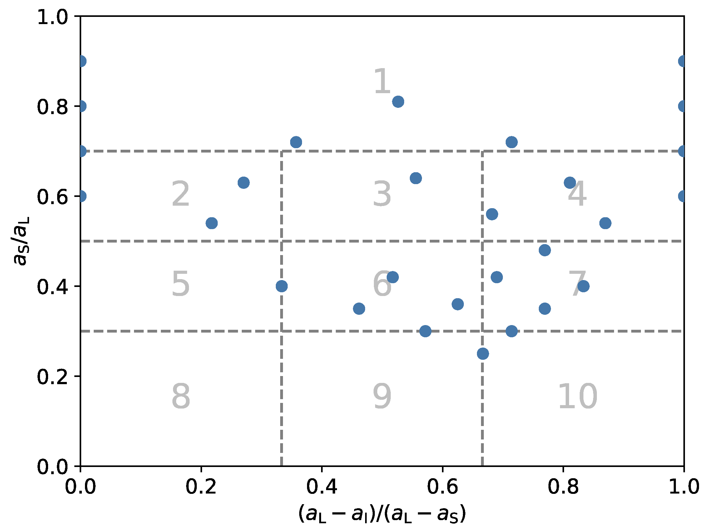
A challenge is the classification of the different shapes. A first approach is categorization in classes. Based on elongation and flatness (defined via main axis lengths), Zingg [5] introduced four different classes (blade, disc, rod and sphere). Sneed and Folk [6] distinguish ten classes, including, in particular, compactness. This, however, does not cover all aspects of shape and further parameters are required. The need for a uniform definition is also reflected in the existence of a specific international standard ISO 9276-6 [7]. Due to the interdependence of many parameters, the construction of a set covering most aspects of shape while also ensuring pairwise independence is complicated. Therefore, Hentschel and Page [8] performed a cluster analysis to identify a minimal set, finding the aspect ratio and a form factor, describing the ruggedness as most important. Later, a more granular classification system with 25 classes was proposed by Blott and Pye [9], also taking the roundness and sphericity into account. To find a correlation applicable to a wide range of shapes, however, there should not be a sharp distinction between classes, but a smooth transition between shapes.

In addition to those parameters, the orientation of the particle is also relevant, as some correlations regarding the settling of particles depend on the crosswise sphericity, which also depends on it. This is, furthermore, of importance in the formation of sediments, as discussed by Allen [10], who stated that the orientation is mainly influenced by the Reynolds number. Sheikh et al. [11] performed simulations to study the orientation of spheroid settling under turbulent conditions. An overview of the orientation of particles for a broad range of Reynolds numbers was given by Bagheri and Bonadonna [12]; for Reynolds numbers up to 100, the particles tend to settle in an orientation which maximizes the drag [13], while many particles have no preferred orientation in the Stokes regime. However, the shape additionally affects the orientation, as shown by Shao et al. [14], who found differences in orientation not only for triangular and rectangular particles, but also for rectangular particles with different aspect ratios for the same Reynolds number.

Extending the drag correlations for spheres [15,16,17] to other particle shapes has been a topic of ongoing research for a long time. McNown [18] proposed a formula for ellipsoids in the Stokes regime in 1950. It is still present in current research, e.g., Sommerfeld and Qadir [19] presented a study investigating the drag and lift depending on the angle of eight particles with different sphericity via lattice Boltzmann simulations in 2018. While the correlation by Leith [20] is restricted to the Stokes regime, it is based on the differentiation between form and friction drag, which depend on the surface tangential and are normal to the settling direction. This differentiation is also visible in later works by Ganser [21], Loth [22], and Hölzer and Sommerfeld [23]. Most correlations are, therefore, based on a similar model with values fitted according to predominantly experimental, but also analytical data. The calculation of drag correction factors for the Stokes and Newton regime, used in the correlations, is common. Bagheri and Bonadonna [12] introduced the additional requirement that shape parameters need to be accessible without extensive measurement effort. They concluded with a correlation solely based on the axis lengths, volume and density ratio, thereby omitting the otherwise commonly used sphericity. Their correlation, together with the one presented by Hölzer and Sommerfeld [23], is among the best performing correlations currently available in the literature for a wide range of Reynolds numbers and shapes. However, all presented correlations mimic a similar structure, based on the assumptions by Leith [20], only modifying terms and adding parameters and further correction terms. This leads to the situation where, even for the best models, a remaining spread is visible, which is not explained by the correlation. As hinted by Bagheri and Bonadonna [12], the range of considered shape parameters needs to be extended to capture more effects; this was also found by Tran-Cong et al. [24].

Depending on the considered particles, more specific correlations are available. Dellino et al. [25] and Dioguardi and Mele [26] presented correlations for pumice particles, namely samples of material from eruptions at the Vesuvius and Camp Flegrei volcanoes. Since the topic of settling non-spherical particles proved to be complex and affected by many factors, investigations of such specific sets as well as additional effects are sensible. For the latter, Hölzer and Sommerfeld [27] investigated, among other things, the influence of the Magnus effect. Few investigations exist which do not correlate the drag coefficient with a Reynolds number, but aim to directly describe the terminal settling velocity. The correlations considered here are the ones by Haider and Levenspiel [28] and Dellino et al. [25]. Such correlations, in addition to being an easy, accessible, a-priori estimate for the terminal settling velocity, might help to improve other models. A broad range of investigations of particle behavior, e.g., in the lung [29,30] or in mixing processes [31], could benefit from such models. For such more specific applications, a tool to obtain correlations, best fit for the considered purpose and the available data, might be more beneficial than a general correlation aiming to describe all cases.

Furthermore, the quality and abundance of data are crucial for a regression analysis and model development. Experimental data might be expensive to obtain, especially in large scales, since one has to measure all relevant parameters for existing particles. This is also discussed by Bagheri and Bonadonna [12], who restricted the model to shape parameters that are easily accessible. This is handy for application, since the required data of a new particle system can be obtained comparably simply, and increases the amount of available datapoints; however, some not-captured effects might be related to more sophisticated shape parameters.

The aim of this work is to provide a tool capable of delivering drag correlations with a good fit for a given set of data, and also apply it to the results of simulations yielding correlations for the drag coefficient and terminal settling velocity. The available literature usually only addresses new correlations, based on the modification and extension of existing models, which are obtained by extending the data basis. This work takes a data-driven approach, obtaining a database not through experimental studies, but through simulations. Depending on the availability of computational resources and preexisting models and implementations, simulations of arbitrarily shaped particles [32] might be an efficient alternative, with the information regarding the settling behavior of the particles becoming more accessible. Therefore, the procedure described in this work allows for a larger database to be obtained, along with advances in available computing power and algorithmics.

Here, the particles were modeled by superellipsoids, as this allows for the depiction of a broad range of shapes. Since the particle shapes can be analytically described, a vast amount of shape parameters can be calculated, which might not be accessible to experimental measurement devices. Therefore, in this work, multiple shape parameters besides axis length, elongation, flatness and sphericity are considered, such as roundness, convexity and further constructed parameters like the Corey shape factor [18], which are displayed in Section 2.2. The considered parameters are also evaluated regarding their relevance during the investigation. As with this representation via superellipsoids, edges are usually, at least to some extent, rounded and not sharp, except for extreme values; this reflects the nature of real particle systems, since corners and edges are usually rounded due to collisions. Therefore, 200 particles, with different shapes and densities, were simulated individually in this work. The shapes were constructed to provide a dataset with preferably equally distributed shape parameters, to reduce the effect of a stronger weighting of a specific class of particles.

One aim of this study is to find a new, improved correlation in a constructive way, by applying a polynomial regression and investigating the statistical relevance of various existing shape parameters and their interactions. To the knowledge of the authors, such an investigation has not been performed before, especially also considering the multicollinearity and statistical relevance of each term by various measures. In addition, a correlation for the terminal settling velocity is proposed.

The simulations were performed applying the homogenized lattice Boltzmann method (HLBM), introduced by Krause et al. [33] and validated in a previous work by Trunk et al. [34]. It is used within the open-source C++ simulation framework OpenLB [35,36].

The remainder of this work is organised as follows. In Section 2, the model for the settling of particles is given as well as an overview of relevant existing drag correlations for spheres and non-spherical particles. The shape parameters considered in this work are defined and the depiction of particles by superellipsoids is described. Following this, in Section 3, the necessary information regarding the applied simulation method and the generation process of the particle dataset is given. In Section 3.2, the applied statistical tools, later applied in the investigation, are introduced. Finally, in Section 4, the conduction and validation of numerical experiments is discussed, and the results are presented in Section 5. The latter is divided into a general inspection of results (Section 5.1), and the regression analyses regarding the drag coefficient (Section 5.2.1) and the terminal settling velocity (Section 5.2.2). A brief overview of the findings is then given in the conclusion in Section 6.

2. Mathematical Modeling

In this work, the behavior of single settling particles in a liquid is studied. Since this is similar to previous studies, this rather general part of the section strongly follows the one given in the preceding publication by Trunk et al. [34]. The dynamic behavior of the system is defined by the motion of the particle and the fluid. The latter is governed by the incompressible Navier–Stokes equations

$$\begin{array}{cccc}\hfill \frac{\partial {\mathit{u}}_{\mathrm{f}}}{\partial t}+({\mathit{u}}_{\mathrm{f}}·\nabla ){\mathit{u}}_{\mathrm{f}}-\nu \Delta {\mathit{u}}_{\mathrm{f}}+\frac{1}{{\rho }_{\mathrm{f}}}\nabla p& ={\mathit{F}}_{\mathrm{f}}\hfill & \hfill & \mathrm{in}{\Omega }_{\mathrm{f}}\times I,\hfill \\ \hfill \nabla ·{\mathit{u}}_{\mathrm{f}}& =0\hfill & \hfill & \mathrm{in}{\Omega }_{\mathrm{f}}\times I.\hfill \end{array}$$

(1)

They are defined for a time interval $I\subseteq \mathbb{R}$ on a spatial domain ${\Omega }_{\mathrm{f}}$ which, together with the area covered by the particle ${\Omega }_{\mathrm{p}}$, spans the computational domain ${\Omega }_{\mathrm{f}}\cup {\Omega }_{\mathrm{p}}=\Omega \subseteq {\mathbb{R}}^3$. Since the considered particles are not stationary, it is ${\Omega }_{\mathrm{f}}={\Omega }_{\mathrm{f}}\left(t\right)$ and ${\Omega }_{\mathrm{p}}={\Omega }_{\mathrm{p}}\left(t\right)$. ${\mathit{u}}_{\mathrm{f}}:{\Omega }_{\mathrm{f}}\times I\to {\mathbb{R}}^3$ denotes the fluid velocity, while $p:{\Omega }_{\mathrm{f}}\times I\to \mathbb{R}$ describes the pressure, ${\mathit{\rho }}_{\mathrm{f}}\in {\mathbb{R}}_{>0}$ the fluid’s density and $\nu \in {\mathbb{R}}_{>0}$ its kinematic viscosity. The total force experienced by the fluid is denoted by ${\mathit{F}}_{\mathrm{f}}$, and is solely composed of the hydrodynamic force due to the exchange of momentum with the submersed particle.

The rigid particle’s motion follows Newton’s second law of motion

$$m_{\mathrm{p}}\frac{d{\mathit{u}}_{\mathrm{p}}}{dt}={\mathit{F}}_{\mathrm{p}}\mathrm{and}\frac{d\left({\mathit{J}}_{\mathrm{p}}{\mathbf{\omega }}_{\mathrm{p}}\right)}{dt}={\mathbf{T}}_{\mathrm{p}}.$$

(2)

Here, $m_{\mathrm{p}}\in {\mathbb{R}}_{>0}$ is the particle’s mass, ${\mathit{u}}_{\mathrm{p}}:I\to {\mathbb{R}}^3$ the particle’s velocity and ${\mathit{F}}_{\mathrm{p}}:I\to {\mathbb{R}}^3$ the force acting on the particle. The rotation can be described in an equivalent way to the moment of inertia ${\mathit{J}}_{\mathrm{p}}\in {\mathbb{R}}^3$, the angular velocity ${\mathbf{\omega }}_{\mathrm{p}}:I\to {\mathbb{R}}^3$ and the torque ${\mathbf{T}}_{\mathrm{p}}:I\to {\mathbb{R}}^3$. Together with an expression for the force ${\mathit{F}}_{\mathrm{p}}$, this enables the calculation of a particle’s trajectory.

The only external forces relevant in this work are the gravitational and buoyancy forces, given by ${\mathit{F}}^{\mathrm{BG}}=(0,0,m_{\mathrm{p}}(1-\frac{{\mathit{\rho }}_{\mathrm{f}}}{{\mathit{\rho }}_{\mathrm{p}}})g)$. The gravitational acceleration of g is equal to $9.81 \mathrm{m}{\mathrm{s}}^{-2}$ throughout this paper. Since only a single particle is considered, contact forces are neglected. Therefore, with the hydrodynamic force ${\mathit{F}}^{\mathrm{H}}:I\to {\mathbb{R}}^3$, responsible for the momentum transfer between fluid and particle, and the vector $\mathbf{r}\in {\mathbb{R}}^3$ yielding the distance to the center of mass for a point in the particle, the force in Equation (2) is given by

$$\begin{array}{cc}\hfill {\mathit{F}}_{\mathrm{p}}& ={\mathit{F}}^{\mathrm{BG}}+{\int }_S\left[-p\mathit{I}+\frac{1}{\mathrm{Re}}(\nabla {\mathit{u}}_{\mathrm{f}}+\nabla {\mathit{u}}_{\mathrm{f}}^t)\right]·\mathit{n}dS,\hfill \\ \hfill {\mathbf{T}}_{\mathrm{p}}& ={\int }_S\mathbf{r}\times \left[-p\mathit{I}+\frac{1}{\mathrm{Re}}(\nabla {\mathit{u}}_{\mathrm{f}}+\nabla {\mathit{u}}_{\mathrm{f}}^t)\right]·\mathit{n}dS,\hfill \end{array}$$

(3)

with $\mathit{n}$ being the normal on the surface S of an object.

2.1. Drag Coefficient

The force mainly responsible for interaction between particle and fluid is the drag force, which depends on the relative velocity between the considered object and the surrounding fluid. In general, it is given by

$${\mathit{F}}^{\mathrm{D}}=\frac{1}{2}{\mathit{\rho }}_{\mathrm{f}}{({\mathit{u}}_{\mathrm{p}}-{\mathit{u}}_{\mathrm{f}})}^2{C}_{\mathrm{D}}A,$$

(4)

with A denoting the projected surface of the considered object in the direction of the relative flow. The drag coefficient $C_{\mathrm{D}}$ depends on the shape of the particle [24,37], but mainly on the Reynolds number

$$\mathrm{Re}=\frac{d_{\mathrm{eq}}{u}_{\mathrm{ts}}}{\nu },$$

(5)

with the terminal settling velocity $u_{\mathrm{ts}}$. In this work, the diameter of the volume equivalent sphere $d_{\mathrm{eq}}$, described in the next section, is used as characteristic length. This allows the calculation of $\mathrm{Re}$ for arbitrary shapes.

For the simple shape of a sphere, numerous correlations for $C_{\mathrm{D}}$ have been proposed based on experimental and analytical investigations [38]. This has already been investigated by the authors in a previous work [34]. The most common correlation is given by Stokes [15] for $\mathrm{Re}<1$ with $C_{\mathrm{D},\mathrm{S}}=24/\mathrm{Re}$. Inserting this in Equation (4), and assuming a force balance, as stated in Equation (3), this leads to the terminal settling velocity

$$u_{\mathrm{ts},\mathrm{S}}=\sqrt{\frac{4}{3}\frac{g{d}_{\mathrm{eq}}}{C_{\mathrm{D},\mathrm{S}}}\frac{{\rho }_{\mathrm{p}}-{\rho }_{\mathrm{f}}}{{\rho }_{\mathrm{f}}}}.$$

(6)

Another common drag correlation for Reynolds numbers up to 800 has been proposed by Schiller and Naumann [16]. It is given by

$$C_{\mathrm{D},\mathrm{SN}}=\frac{24}{\mathrm{Re}}\left(1+0.15{\mathrm{Re}}^{0.687}\right),$$

(7)

and has been extended by Clift and Gauvin [17] for the full intermediate and Newton regime by

$$C_{\mathrm{D},\mathrm{CG}}=\frac{24}{\mathrm{Re}}\left(1+0.15{\mathrm{Re}}^{0.687}\right)+0.42{\left(1+\frac{42500}{{\mathrm{Re}}^{1.16}}\right)}^{-1}.$$

(8)

2.2. Shape Parameter

Some of the challenges in the selection of particle shape parameters are caused by the numerous ways of defining the measures and the correlation between the parameters. Additionally, since a particle’s shape can be arbitrarily complex, it cannot be fully described by a small set of values, which usually are not fully independent of each other. In this section, the measures used in this work are briefly introduced.

A first approach is the definition of the diameter of a sphere with a volume equal to the one of the particle $V_{\mathrm{p}}$. It is given by

$$d_{\mathrm{eq}}=\sqrt[3]{\frac{6}{\pi }{V}_{\mathrm{p}}}.$$

(9)

Since this parameter alone does not carry any information about the shape, additional values like the aspect ratio, defined as the ratio of minimum to maximum of the Feret diameter, are required. In previous studies by the authors [39], it was shown that this parameter is still too generic; therefore, it is split in elongation

$$E=a_{\mathrm{I}}/a_{\mathrm{L}},$$

(10)

and flatness

$$F=a_{\mathrm{S}}/a_{\mathrm{I}},$$

(11)

in this work. Here, $a_{\mathrm{L}}$, $a_{\mathrm{I}}$ and $a_{\mathrm{S}}$ denote the longest, intermediate and shortest half-axis of the particle, respectively.

Another common parameter is the convexity ${\kappa }_{\mathrm{con}}$, defined as the ratio of the particle’s volume to the volume of its convex hull, taking values between 0 and 1. The sphericity $\psi$, as defined by Wadell [40], has already been used in many studies regarding the particle shape [19,23]. It also takes values between 0 and 1, with the latter being a perfect sphere. Defined as the ratio between the surface of a volume-equivalent sphere and the particle’s surface $A_{\mathrm{p}}$, it is given as

$$\psi =\frac{1}{A_{\mathrm{p}}}\sqrt[3]{\pi {\left(6V_{\mathrm{p}}\right)}^2}.$$

(12)

While the sphericity describes the particle’s resemblance to a sphere, the roundness ${\kappa }_{\mathrm{rnd}}$ is related to the curvature of its corners and edges. While the definition based on the measurements by Krumbein [41] or by Wadell [40] are rather inconvenient to calculate, it is defined here as

$${\kappa }_{\mathrm{rnd}}=\frac{V_{\mathrm{p}}}{A_{\mathrm{p}}{\left(8a_{\mathrm{L}}{a}_{\mathrm{I}}{a}_{\mathrm{S}}\right)}^{1/3}}.$$

(13)

This formula was proposed by Hayakawa and Oguchi [42], who found a strong correlation with the results by Krumbein [41].

Further parameters can be created, e.g., by combining the lengths of the main axes. A common parameter is the Corey shape factor ${\lambda }_{\mathrm{CSF}}$ [18,43], yielding lower values with a flatter particle. It is defined by

$${\lambda }_{\mathrm{CSF}}=\frac{a_{\mathrm{S}}}{\sqrt{a_{\mathrm{I}}{a}_{\mathrm{L}}}}.$$

(14)

The Hofmann shape entropy ${\lambda }_{\mathrm{H}}$ [44], which was found to properly describe the dynamics of settling ellipsoids [45], is defined in a more complex way as

$${\lambda }_{\mathrm{H}}=-\frac{{\tilde{a}}_{\mathrm{S}}ln\left({\tilde{a}}_{\mathrm{S}}\right)+{\tilde{a}}_{\mathrm{I}}ln\left({\tilde{a}}_{\mathrm{I}}\right)+{\tilde{a}}_{\mathrm{L}}ln\left({\tilde{a}}_{\mathrm{L}}\right)}{ln\left(3\right)},$$

(15)

for axis lengths normalized as ${\tilde{a}}_i=a_i/(a_{\mathrm{S}}+a_{\mathrm{I}}+a_{\mathrm{L}})$ for $i\in \{S,I,L\}$. Le Roux investigated the settling of grains with a database containing (prolate and oblate) spheroids, discs, cylinders, and ellipsoids, finding correlations for the settling velocity of the particles and also performing a hydrodynamic classification regarding the shape [46]. The found parameter

$${\lambda }_{\mathrm{LR}}={\left(1-\frac{a_{\mathrm{S}}}{a_{\mathrm{L}}}\right)}^{\sigma },$$

(16)

depends on a value $\sigma$ which is dependent of the class of shape; it is given, e.g., by $\sigma =2.5$ for ellipsoids and $\sigma =1.6$ for discs.

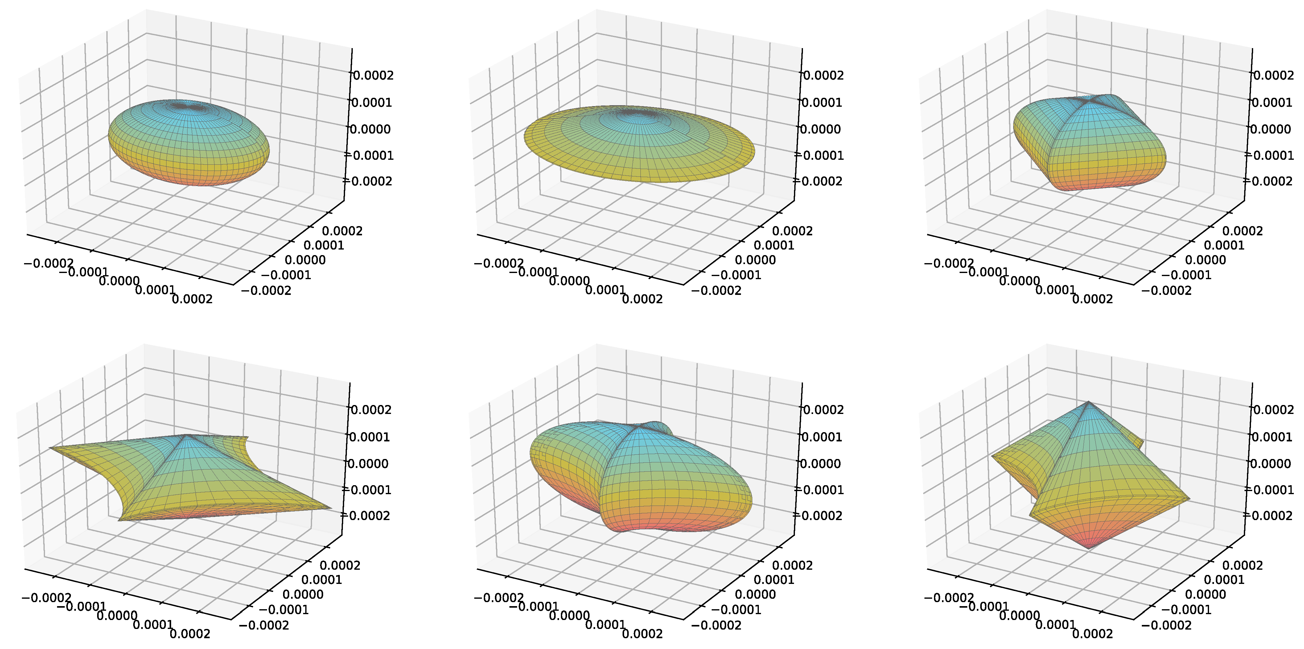
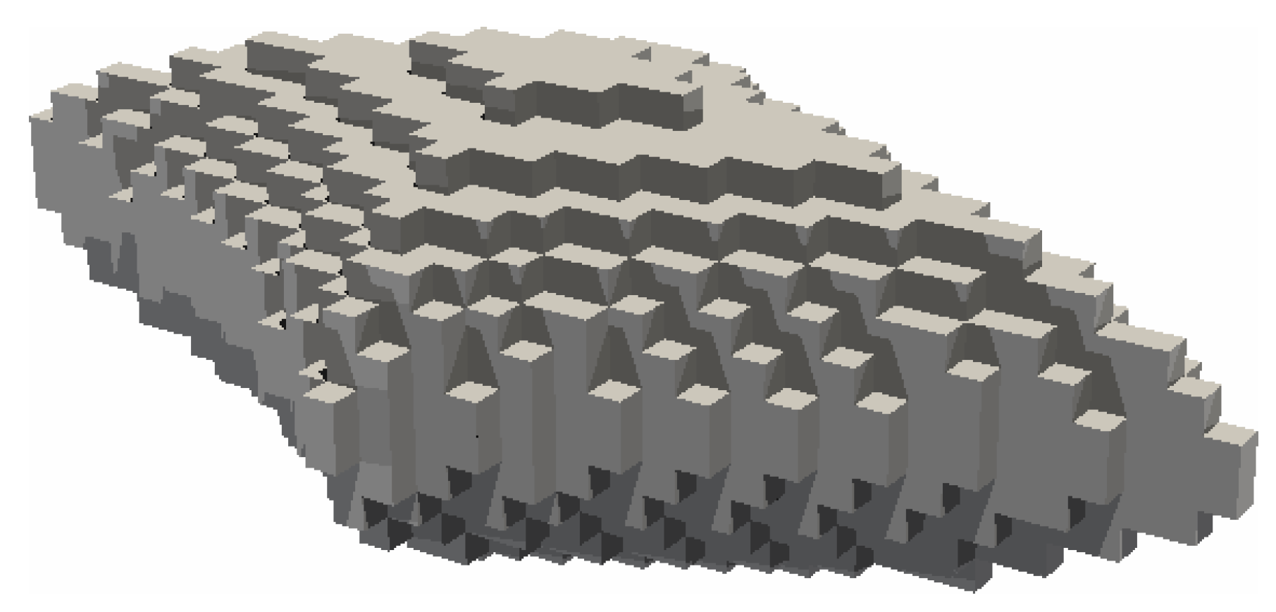
2.3. Particle Representation

For the depiction of arbitrary particle shapes, superellipsoids are chosen in this work, as they represent a compromise between a diversity of possible shapes (e.g., rectangular, spheroidal or cylindrical) and analytical manageability. Information on the modeling parameter and transformations of a superellipsoid are given, e.g., by Williams and Pentland [47] or Barr [48]. Even contact-detection algorithms exist, as presented by Wellmann et al. [49]. An extensive discussion on the geometric properties is given by Jaklič [50].

Let $(X,Y,Z)$ be the coordinates of a point in ${\mathbb{R}}^3$; then, a superellipsoid is described by

$${\left({\left|\frac{X}{a}\right|}^{{\xi }_1}+{\left|\frac{Y}{b}\right|}^{{\xi }_1}\right)}^{{\xi }_2/{\xi }_1}+{\left|\frac{Z}{c}\right|}^{{\xi }_2}\le 1,$$

(17)

for half-axis lengths $a,b,c$ in x-, y- and z-direction, respectively. The exponents ${\xi }_1$ and ${\xi }_2$ control the roundness of the superellipsoid. Considering $a=b=c$, this geometric primitive, e.g., takes on the shape of a sphere for ${\xi }_1={\xi }_2=2$, a cube for ${\xi }_1,{\xi }_2\to \infty$ or the the shape of a cylinder for ${\xi }_1=2$ and ${\xi }_2\to \infty$. Overall, the shape is convex for ${\xi }_1\ge 1$ and tends to be flatter for ${\xi }_2\to 0$.

While Equation (17) allows a description of the surface, the volume and moment of inertia are also required for the simulation. They can be defined utilizing the moments given by Jaklič and Solina [51] as

$$m_{i,j,k}=\frac{2}{i+j+2}{a}^{i+1}{b}^{j+1}{c}^{k+1}{\xi }_1{\xi }_{2}B\left((k+1)\frac{{\xi }_1}{2},(i+j+2)\frac{{\xi }_1}{2}+1\right)B\left((j+1)\frac{{\xi }_2}{2},(i+1)\frac{{\xi }_2}{2}\right),$$

(18)

for $i,j,k\in {\mathbb{N}}_0$. The beta function is given by

$$B(x,y)={\int }_0^1{t}^{x-1}{(1-t)}^{y-1}dt\mathrm{for}x,y>0,$$

(19)

or can alternatively be represented as combination of gamma functions. Based on Equation (18), the volume $V_{\mathrm{p}}$ and the moment of inertia ${\mathit{J}}_{\mathrm{p}}=(J_{xx},J_{yy},J_{zz})$ are now defined as

$$V_{\mathrm{p}}=m_{0,0,0},$$

(20)

$$J_{xx}=m_{0,2,0}+m_{0,0,2},$$

(21)

$$J_{yy}=m_{2,0,0}+m_{0,0,2},$$

(22)

$$J_{zz}=m_{2,0,0}+m_{0,2,0}.$$

(23)

2.4. Drag Correlations for Non-Spherical Particles

There have been many attempts to find and improve a drag correlation for different particle shapes and different ranges of Reynolds numbers. The oldest discussed here is derived by Leith [20] for the Stokes region. Considering the form drag originating from pressure on the particle’s surface and friction drag caused by a tangential shear stress, Leith proposed a formula based on the diameter of a surface-equivalent sphere and the diameter of a sphere with the same projected area in the direction of motion. His parameters were later interpreted as sphericity $\psi$ and crosswise sphericity ${\psi }_{\perp }$, i.e., the ratio of projected area of a volume-equivalent sphere to the projected area of the particle normal to the direction of motion, leading to the most commonly used version

$$K_{\mathrm{S}}=\frac{1}{3}\sqrt{{\psi }_{\perp }}+\frac{2}{3}\sqrt{\psi }.$$

(24)

Here, $K_{\mathrm{S}}$ denotes the drag correction factor for a particle in the Stokes regime regarding a volume-equivalent sphere. As Leith [20] found evaluating his results, these do not fully explain the experimental reference data; he proposed the application of a least-squares fit for additional terms regarding the axis lengths. Likely because these results are specific to the considered data basis, usually, only the formula depicted here is referenced.

Later, Haider and Levenspiel [28] performed a non-linear regression analysis on a data basis of 409 polyhedrons and 87 discs for Reynolds numbers up to $2.6\times {10}^5$. The result is the comparably complex formulation of

$$\begin{array}{cc}\hfill C_{\mathrm{D},\mathrm{HL}}=\frac{24}{\mathrm{Re}}& (1+c_1{\mathrm{Re}}^{{\mathrm{c}}_2})+\frac{{\mathrm{c}}_3}{1+{\mathrm{c}}_4/\mathrm{Re}},\mathrm{with}\hfill \\ \hfill c_1& =e^{2.329-6.458\psi +2.449{\psi }^2},\hfill \\ \hfill c_2& =0.096+0.557\psi ,\hfill \\ \hfill c_3& =e^{4.905-13.894\psi +18.422{\psi }^2-10.260{\psi }^3},\hfill \\ \hfill c_4& =e^{1.468+12.258\psi -20.732{\psi }^2+15.886{\psi }^3}.\hfill \end{array}$$

(25)

The error for the disc-like particles was found to be approximately four times the one of the polyhedral particles, probably due to the unbalanced data basis. In addition, Haider and Levenspiel [28] proposed a formulation to estimate the terminal settling velocity for isometric particles with a sphericity between $0.5$ and 1, by

$$\begin{array}{cc}\hfill u_{\mathrm{ts},\mathrm{HL}}& ={\left(\frac{g\nu ({\rho }_{\mathrm{p}}-{\rho }_{\mathrm{f}})}{{\rho }_{\mathrm{f}}}\right)}^{1/3}{\left(\frac{18}{d_{*}^2}+\frac{2.335-1.744\psi }{\sqrt{d_{*}}}\right)}^{-1},\mathrm{with}\hfill \\ \hfill d_{*}& =d_{eq}{\left(\frac{g({\rho }_{\mathrm{p}}-{\rho }_{\mathrm{f}})}{{\nu }^2{\rho }_{\mathrm{f}}}\right)}^{1/3}.\hfill \end{array}$$

(26)

A study by Ganser [21] considering 731 datapoints aggregated from the literature concluded with

$$\begin{array}{cc}\hfill C_{\mathrm{D},\mathrm{G}}& =\frac{24K_{\mathrm{S}}}{\mathrm{Re}}\left(1+0.1118{\left(\frac{\mathrm{Re}{K}_{\mathrm{N}}}{K_{\mathrm{S}}}\right)}^{0.6567}\right)+\frac{0.4305K_{\mathrm{N}}}{1+3305K_{\mathrm{S}}/\left(\mathrm{Re}{K}_{\mathrm{N}}\right)},\mathrm{with}\hfill \\ \hfill K_{\mathrm{S}}& =\frac{1}{3}+\frac{2}{3}\sqrt{\psi },\hfill \\ \hfill K_{\mathrm{N}}& ={10}^{1.8148{(-log\psi )}^{0.5743}}.\hfill \end{array}$$

(27)

As well as the new correction factor for the Stokes regime, an additional one was introduced for the Newton regime, along with the assumption that these two factors are sufficient for an adequate prediction of the drag coefficient for Reynolds numbers up to $\mathrm{Re}{K}_{\mathrm{S}}{K}_{\mathrm{N}}\le {10}^5$. While the formula presented here is mainly applicable to isometric objects, alternatives for disc-like particles were also presented; however, these require knowledge of the orientation of the particle. These shape-dependent differences were found to mainly affect $K_{\mathrm{S}}$. Ganser [21] further concluded that the introduction of a third parameter for the intermediate regime could reduce the remaining variance.

Loth [22] extended the investigations of Ganser [21] and Leith [20], also providing a more differentiated discussion on the behavior in the intermediate Reynolds number regime. Their finding was that different formulations are required regarding the circularity of the projected area of the particle in the direction of motion. This, of course, also required knowledge of orientation. Despite this, an additional correction factor for the Stokes regime

$$K_{\mathrm{S}}={\left(\frac{a_{\mathrm{L}}{a}_{\mathrm{I}}}{a_{\mathrm{S}}^2}\right)}^{0.09}={\left(\frac{1}{{\lambda }_{\mathrm{CSF}}^2}\right)}^{0.09},$$

(28)

was proposed, describing irregular particles.

To incorporate the particle orientation without differentiation between shape classes, Hölzer and Sommerfeld [23] proposed taking the lengthwise sphericity ${\psi }_{\Vert }$, defined as “the ratio between the cross-sectional area of the volume equivalent sphere and the difference between half the surface area and the mean longitudinal (i.e., parallel to the direction of relative flow) projected cross-sectional area of the considered particle” [23] into account. Their correlation, which was evaluated on 2061 datapoints, is given by

$$C_{\mathrm{D},\mathrm{HS}}=\frac{8}{\mathrm{Re}\sqrt{{\psi }_{\Vert }}}+\frac{16}{\mathrm{Re}\sqrt{\psi }}+\frac{3}{\sqrt{\mathrm{Re}}{\psi }^{3/4}}+0.{421}^{0.4{(-log\psi )}^{0.2}}\frac{1}{{\psi }_{\perp }},$$

(29)

and showed a tremendous improvement in the prediction of the drag coefficient for disc-like objects. They also showed that replacing lengthwise with crosswise sphericity only leads to a drop in the mean deviation from $14.1\%$ to $14.4\%$ from the experimental results.

Finally, Bagheri and Bonadonna [12] compiled a large dataset of 2166 particles from the literature and their own experiments across sub-critical Reynolds numbers, paired with analytical data for ${10}^4$ ellipsoids in the Stokes regime. Based on the assumption by Ganser [21], they concluded with a formula based on Stokes and Newton correction factors

$$\begin{array}{cc}\hfill C_{\mathrm{D},\mathrm{BB}}& =\frac{24K_{\mathrm{S}}}{\mathrm{Re}}\left(1+0.125{\left(\frac{\mathrm{Re}{K}_{\mathrm{N}}}{K_{\mathrm{S}}}\right)}^{2/3}\right)+\frac{0.46K_{\mathrm{N}}}{1+5330/(\mathrm{Re}{K}_{\mathrm{N}}/K_{\mathrm{S}})},\mathrm{with}\hfill \\ \hfill K_{\mathrm{S}}& =0.5\left(F_{\mathrm{S}}^{1/3}+F_{\mathrm{S}}^{-1/3}\right),\hfill \\ \hfill K_{\mathrm{N}}& ={10}^{c_1{(-log{F}_{\mathrm{N}})}^{c_2}},\hfill \\ \hfill c_1& =0.45+\frac{10}{e^{2.5log{\rho }^{\prime }}+30},\hfill \\ \hfill c_2& =1-\frac{37}{e^{3log{\rho }^{\prime }}+100},\hfill \\ \hfill F_{\mathrm{S}}& =F{E}^{1.3}\frac{d_{eq}^3}{a_{\mathrm{S}}{a}_{\mathrm{I}}{a}_{\mathrm{L}}},\hfill \\ \hfill F_{\mathrm{N}}& =F^{2}E\frac{d_{eq}^3}{a_{\mathrm{S}}{a}_{\mathrm{I}}{a}_{\mathrm{L}}}.\hfill \end{array}$$

(30)

The formula here is not taken directly from the publication, but a corrected version by Bagheri and Bonadonna [52]. They further argued that the sphericity, in addition to being harder to measure, is inferior to a shape descriptor based on the axis lengths. In an extensive discussion of particle behavior in the Stokes and Newton regime, it was found that the density ratio ${\rho }^{\prime }$ is also relevant, especially in the Newton regime. This is supported by various studies, suggesting that the trajectory might change depending on the density ratio [53,54,55]. A comparison showed their formula yielded the lowest deviation across all correlations discussed up to this point, and thereby is currently among the best-performing, together with the one proposed by Hölzer and Sommerfeld [23], to the knowledge of the authors. However, a spread in results is still visible. This hints that further effects and parameters might need to be considered to further improve the formulation.

More specific to a set of pumice particles from volcanic eruptions, Dioguardi and Mele [26] proposed a correlation depending on the drag coefficient for spheres, computed according to Clift and Gauvin [17], and the ratio of sphericity to circularity $\varphi$. The latter is given as ratio of maximum projected area to the projected area of a volume-equivalent sphere. Their formula finally reads

$$C_{\mathrm{D},\mathrm{DM}}=\frac{C_{\mathrm{D},\mathrm{CG}}}{{\mathrm{Re}}^2{(\psi /\varphi )}^{{\mathrm{Re}}^{-0.23}}}{\left(\frac{\mathrm{Re}}{1.1883}\right)}^{1/0.4826}.$$

(31)

Dellino et al. [25] used the same dataset to develop a direct correlation between the terminal settling velocity and particle parameters, also relying on the ratio between sphericity and circularity. This is given by

$$u_{\mathrm{ts},\mathrm{D}}=\frac{1.2065\nu }{d_{\mathrm{eq}}}{\left(\frac{d_{\mathrm{eq}}^{3}g({\rho }_{\mathrm{p}}-{\rho }_{\mathrm{f}}){(\psi /\varphi )}^{1.6}}{{\nu }^2{\rho }_{\mathrm{f}}}\right)}^{0.5206}.$$

(32)

This allows for a direct estimation of the terminal settling velocity without the need for an iterative algorithm, as is required when using the correlations regarding the drag coefficient.

3. Numerical and Statistical Methods

For the numerical simulations in this paper, the homogenized lattice Boltzmann method is applied. The method and implementation have been extensively tested and validated in a previous publication by Trunk et al. [34]; therefore, only the relevant parts are summarized here.

The HLBM was first proposed by Krause et al. [33] and later updated by Trunk et al. [34]. In this work, the version used in the latter publication is used, which is based on a forcing scheme by Kupershtokh et al. [56] and the momentum exchange algorithm by Wen et al. [57]. The extension to 3D and the incorporation of arbitrary particle shapes was described by Trunk et al. [32]. A setup similar to the one used in this work was studied by Trunk et al. [34] for spheres, yielding an error of approximately $6\%$ compared to the drag correlation by Schiller and Naumann [16] and approximately $3\%$ to the drag correlation by Abraham [58].

Since this approach is a specialisation of the more general lattice Boltzmann method (LBM), all values are non-dimensionalized by the spatial and temporal discretization parameter $\delta x$ and $\delta t$ and the density ${\rho }_{\mathrm{f}}$ during processing. The resulting system is denoted as a “lattice system”. It was found by Trunk et al. [34] that the quality of the results depends on the maximal occurring velocity in the lattice system $u_{\max }^{\mathrm{L}}$ for the investigation of settling processes, defined by

$$u_{\max }^{\mathrm{L}}=\frac{\delta t}{\delta x^2}{u}_{\max },$$

(33)

with $u_{\max }$ as the maximum fluid velocity observed in the simulation. For a sufficiently low error, $u_{\max }^{\mathrm{L}}$ should be smaller than $0.04$. A further condition exists regarding the lattice relaxation time

$$\tau =\nu \frac{\delta t}{\delta x}\frac{1}{c_{\mathrm{s}}^2}+0.5,$$

(34)

where $c_{\mathrm{s}}^2$ is the lattice speed of sound [59]. For the simulation to be stable, $\tau$ may not be too close to $0.5$. For further information on the LBM, the interested reader is referred to Krüger et al. [59].

3.1. Particle Generation

According to the approach described in Section 2.3, a particle is defined by 5 parameters. To create a collection, parameter ranges are defined, for which the half-axis lengths are defined via elongation and flatness, starting with $a=0.01\mathrm{m}$. Varying the particle’s density, the parameters

$$\begin{array}{cc}\hfill E& \in \{0.5,0.6,0.7,0.8,0.9,1\},\hfill \\ \hfill F& \in \{0.5,0.6,0.7,0.8,0.9,1\},\hfill \\ \hfill {\xi }_1& \in \{8,2,1,0.933,0.9,0.866,0.833,0.8,0.766,0.733,0.7,0.666\},\hfill \\ \hfill {\xi }_2& \in \{8,2,1\},\hfill \\ \hfill {\rho }_{\mathrm{p}}& \in \{2360 \mathrm{k}\mathrm{g}{\mathrm{m}}^{-3},2460 \mathrm{k}\mathrm{g}{\mathrm{m}}^{-3},2560 \mathrm{k}\mathrm{g}{\mathrm{m}}^{-3},2660 \mathrm{k}\mathrm{g}{\mathrm{m}}^{-3},2760 \mathrm{k}\mathrm{g}{\mathrm{m}}^{-3}\},\hfill \end{array}$$

(35)

lead to a group of 6480 particles. For comparability, the half-axes of all generated objects are scaled equally, such that the resulting particle has a volume of $1.66742\times {10}^{-11}$ $\mathrm{m}$${}^3$. Thereby, the equivalent sphere diameter of all generated particles is $d_{\mathrm{eq}}=3.1697\times {10}^{-4} \mathrm{m}$. During the creation process, all shape parameters given in Section 2.2 are calculated along with the volume, according to Equation (20). Furthermore, the terminal settling velocity obtained using the drag correlation by Stokes (Equation (6)) and the surface are computed. For the latter, a triangulation of the parametric representation in terms of the modified spherical coordinates of Equation (17) is used [51].

From this set of particles, 200 are selected, such that a chi-squared test [60] for an equal distribution of frequencies yields a p-value above $0.99$ for all considered parameters; some of them are shown in Figure 1. The frequencies are given for a sensible choice of numbers of bins for each parameter, as shown in

Table 1. Results of a chi-squared test for equal distribution of frequencies of different shape parameters.

	Elongation	Flatness	Convexity	Sphericity	Density
numberof bins	6	6	6	5	5
p-value	$0.998$	$0.995$	$0.999$	$1.000$	$1.000$

. For the density, 5 bins wwere used, as only this number of discrete values is considered. For reference, the data and parameters for all 200 particles are given in Appendix A.

As a first step, the Pearson correlation coefficients [60,61] for the shape parameters are calculated; their absolute values are depicted in

Table 2. Absolute Values of the correlation coefficients according to Pearson [61] for the considered shape parameters.

	${\mathit{a}}_{\mathbf{L}}$	${\mathit{a}}_{\mathit{I}}$	${\mathit{a}}_{\mathbf{S}}$	${\mathit{\xi }}_1$	${\mathit{\xi }}_2$	${\mathit{\rho }}_{\mathbf{p}}$	E	F	${\mathit{\kappa }}_{\mathbf{con}}$	$\mathit{\psi }$	${\mathit{\psi }}_{\perp }$	${\mathit{\kappa }}_{\mathbf{rnd}}$	${\mathit{\lambda }}_{\mathbf{CSF}}$	${\mathit{\lambda }}_{\mathbf{H}}$	${\mathit{\lambda }}_{\mathbf{LR}}$
$a_{\mathrm{L}}$	$1.0$	$0.55$	$0.04$	$0.41$	$0.17$	$0.03$	$0.74$	$0.51$	$0.65$	$0.52$	$0.64$	$0.68$	$0.67$	$0.73$	$0.75$
$a_{\mathrm{I}}$	$0.55$	$1.0$	$0.57$	$0.39$	$0.47$	$0.08$	$0.13$	$0.13$	$0.63$	$0.61$	$0.47$	$0.85$	$0.05$	$0.04$	$0.02$
$a_{\mathrm{S}}$	$0.04$	$0.57$	$1.0$	$0.18$	$0.57$	$0.03$	$0.44$	$0.72$	$0.41$	$0.45$	$0.31$	$0.61$	$0.73$	$0.64$	$0.65$
${\xi }_1$	$0.41$	$0.39$	$0.18$	$1.0$	$0.02$	$0.08$	$0.19$	$0.15$	$0.47$	$0.44$	$0.31$	$0.57$	$0.18$	$0.21$	$0.21$
${\xi }_2$	$0.17$	$0.47$	$0.57$	$0.02$	$1.0$	$0.03$	$0.16$	$0.36$	$0.07$	$0.05$	$0.23$	$0.34$	$0.34$	$0.32$	$0.31$
${\rho }_{\mathrm{p}}$	$0.03$	$0.08$	$0.03$	$0.08$	$0.03$	$1.0$	$0.02$	$0.1$	$0.03$	$0.05$	$0.04$	$0.05$	$0.08$	$0.02$	$0.03$
E	$0.74$	$0.13$	$0.44$	$0.19$	$0.16$	$0.02$	$1.0$	$0.45$	$0.33$	$0.2$	$0.47$	$0.17$	$0.72$	$0.85$	$0.84$
F	$0.51$	$0.13$	$0.72$	$0.15$	$0.36$	$0.1$	$0.45$	$1.0$	$0.07$	$0.01$	$0.0$	$0.01$	$0.94$	$0.79$	$0.83$
${\kappa }_{\mathrm{con}}$	$0.65$	$0.63$	$0.41$	$0.47$	$0.07$	$0.03$	$0.33$	$0.07$	$1.0$	$0.93$	$0.75$	$0.86$	$0.17$	$0.22$	$0.23$
$\psi$	$0.52$	$0.61$	$0.45$	$0.44$	$0.05$	$0.05$	$0.2$	$0.01$	$0.93$	$1.0$	$0.73$	$0.86$	$0.08$	$0.1$	$0.12$
${\psi }_{\perp }$	$0.64$	$0.47$	$0.31$	$0.31$	$0.23$	$0.04$	$0.47$	$0.0$	$0.75$	$0.73$	$1.0$	$0.74$	$0.18$	$0.2$	$0.23$
${\kappa }_{\mathrm{rnd}}$	$0.68$	$0.85$	$0.61$	$0.57$	$0.34$	$0.05$	$0.17$	$0.01$	$0.86$	$0.86$	$0.74$	$1.0$	$0.06$	$0.08$	$0.11$
${\lambda }_{\mathrm{CSF}}$	$0.67$	$0.05$	$0.73$	$0.18$	$0.34$	$0.08$	$0.72$	$0.94$	$0.17$	$0.08$	$0.18$	$0.06$	$1.0$	$0.92$	$0.95$
${\lambda }_{\mathrm{H}}$	$0.73$	$0.04$	$0.64$	$0.21$	$0.32$	$0.02$	$0.85$	$0.79$	$0.22$	$0.1$	$0.2$	$0.08$	$0.92$	$1.0$	$0.99$
${\lambda }_{\mathrm{LR}}$	$0.75$	$0.02$	$0.65$	$0.21$	$0.31$	$0.03$	$0.84$	$0.83$	$0.23$	$0.12$	$0.23$	$0.11$	$0.95$	$0.99$	$1.0$

. The results show three clusters of strong correlation. Firstly the constructed shape factors, i.e., the Corey shape factor, the Hofmann shape entropy and the Le Roux shape parameter; this is to be expected, as all of them depend on the axis lengths of the investigated objects. This also explains the second correlation between the first cluster and the elongation and flatness. The third group contains the convexity, sphericity and roundness. This suggests that adding more than one of these parameters to a model will have a weaker influence on the quality of the results. Lastly, a weaker correlation between this third cluster and the exponent ${\xi }_1$ used in the particle creation process can be observed. Furthermore, the axis lengths are correlated to almost every other parameter, except the density, as it is varied independently.

3.2. Statistical Tools

To find the correlation between a dependent variable Y (here, e.g., the drag coefficient) and multiple independent variables $X_i,i\in \{1,\dots ,k;k\in \mathbb{N}\}$ (here e.g., sphericity), often, regression analysis is applied to find a model, yielding approximations of the dependent variable $\widehat{Y}$. The quality of a model is evaluated by the amount of variance in the data it can describe; this is given by the coefficient of determination

$$R^2=1-\frac{{\sum }_{j=1}^n{r}_j^2}{{\sum }_{j=1}^n{(Y_j-\overline{Y})}^2},\mathrm{with}n\in \mathbb{N},$$

(36)

for the residuals $r_j=Y_j-{\widehat{Y}}_j$. Here, $\overline{Y}$ represents the mean and n is the number of datapoints. Considering multiple independent variables, the adjusted version given by

$$R_{\mathrm{a}}^2=1-(1-R^2)\frac{n-1}{n-k-1},$$

(37)

is more appropriate. This further allows the definition of the variance inflation factor $\mathit{VIF}$ as a measure of multicollinearity [62] by

$${\mathit{VIF}}_i=\frac{1}{1-R_i^2},$$

(38)

with $R_i^2$ being the coefficient of determination of a linear regression, choosing $X_i$ as the dependent variable. Values $>10$ are considered critical since they indicate a high level of multicollinearity, which negatively affects the stability of the method chosen to calculate the regression coefficients.

To further obtain an a priori estimation regarding the dependency between two explanatory variables, the mutual information $\mathit{MI}$ introduced by Shannon [63], defined as the difference between the sum of entropy of the two variables and the joint entropy, is calculated. Later, Kraskov et al. [64] introduced an estimate for this, using k-nearest neighbor distances, which is applied in this work. $\mathit{MI}$ reaches its minimum of 0 for strictly independent variables. Another measure is the F-value of a linear regression, with only one explanatory variable regarding the desired dependent variable, given as

$$F_{\mathrm{sample}}=\frac{R^2/k}{(1-R^2)/(n-k-1)}.$$

(39)

A high value indicates the relevance of the explanatory variable in the description of the dependent one [62]; however, this test is more suited to the detection of linear dependency.

To evaluate the significance of an explanatory variable for a performed regression, a t-test is performed. Here, a large t-value implies a high significance of the explanatory variable. Since the values can also be negative, the absolute has to be considered. For the variable $X_i$, with the associated regression coefficient ${\beta }_i$, the score is given as

$$T_{\mathrm{sample}}=\left|{\beta }_i{\left(\frac{\sqrt{{(n-k-1)}^{-1}{\sum }_{j=1}^n{r}_j^2}}{\sqrt{{\sum }_{j=1}^n{(X_{i,j}-{\overline{X}}_i)}^2}}\right)}^{-1}\right|,$$

(40)

for the mean of an explanatory variable for all observations, ${\overline{X}}_i$. With the T-distribution, an additional p-value can be computed to check if a term is significant above a threshold level, usually chosen as $\alpha =0.05$. Another measure to evaluate the significance of an explanatory variable is the permutation importance introduced by Breiman [65]. It requires a score to evaluate the quality of a model, which is here chosen asthe coefficient of determination $R^2$. For each considered variable, the regression is performed five times, with the values of the variable being shuffled each time over the observations, thereby destroying the correlation between feature and dependent variable. The mean $R^2$ across this runs is subtracted from the one obtained with not-permuted data, yielding the permutation importance $\mathit{PI}$.

Finally, the observations are evaluated regarding the regression performed to identify outliers. The first approach is to standardize the residuals: observations yielding an absolute value above three are considered to be outliers. In the following, Cook’s distance

$$d_{\mathrm{Cook}}=\frac{{\sum }_{j=1}^n({\widehat{Y}}_j-{\widehat{Y}}_{j\left(l\right)})}{{(n-k-1)}^{-1}{\sum }_{j=1}^n{r}_j},l\in \{1,\dots ,n\},$$

(41)

is computed to evaluate the influence of an observation on the model. Here, ${\widehat{Y}}_{j\left(l\right)}$ is the approximation of the dependent variable by a model unaware of the l-th observation. For this measure, a value above $0.5$ marks an influential point, while values above 1 indicate an outlier.

4. Numerical Experiments

In this section, some preparatory calculations regarding the starting conditions are presented, as well as the simulation setup for the investigation of settling particles. For the latter, some preliminary studies validating the setup are discussed.

4.1. Preparation

Depending on the Reynolds number, the initial conditions, i.e., the orientation of the particle, should be checked. For low $\mathrm{Re}$, objects tend to keep their angle; for intermediate $\mathrm{Re}$, axis-symmetric particles rotate such that the maximum projected area is normal to the flow or settling direction. Using the equivalent spherical diameter for the Reynolds number and utilising the drag correlation by Schiller and Naumann [16], it can be estimated that $\mathrm{Re}=15.41$ with $\nu ={10}^{-6} {\mathrm{m}}^2{\mathrm{s}}^{-1}$. The later-observed terminal settling velocities lead to Reynolds numbers between $\mathrm{Re}=9.64$ and $\mathrm{Re}=22.86$. As this is in the intermediate regime, the angle for which the projection in settling direction yields the maximum surface is calculated.

For these calculations, a voxel representation of the superellipsoid is used and the projected surface is calculated. To find the maximum, the particle is rotated in $1^{\circ }$ steps around the x-axis and y-axis. Since superellipsoids are rotational symmetric, in this case, around the z-axis, this suffices. This additional information is required to ensure that all objects have the same starting conditions, especially for the investigation of the initial phase of the particle leveling out at its equilibrium position.

4.2. Simulation Setup

For the investigation of single particle settling, the superellipsoids are placed in a domain with $0.007$ $\mathrm{m}$ width and depth and a height of $0.0175$ $\mathrm{m}$, as depicted in Figure 2. The center of mass of the object is initially located in the middle of the domain, $2a_{\max }$ from the top. The latter corresponds to the maximum half-axis length across all particles $a_{\max }=4.777\times {10}^{-4} \mathrm{m}$. For the fluid ${\rho }_{\mathrm{f}}=998 \mathrm{k}\mathrm{g} {\mathrm{m}}^{-3}$ and $\nu ={10}^{-6} {\mathrm{m}}^2 {\mathrm{s}}^{-1}$ is chosen, while the gravitational acceleration is given as $g=9.81\mathrm{m} {\mathrm{s}}^{-1}$.

The discretization is chosen such that the volume-equivalent sphere diameter is resolved by 20 cells; this represents a grid spacing of $\delta x=1.58484\times {10}^{-5} \mathrm{m}$. The resulting domain thereby consists of 215,877,220 cells. Since it was found by Trunk et al. [34] that the maximum occurring lattice velocity should not exceed $0.04$, the temporal discretization is chosen such that the maximum velocity of a volume-equivalent sphere according to Schiller and Naumann [16] equals a lattice velocity of $0.02$, leading to $\delta t=6.51915\times {10}^{-6} \mathrm{s}$. This proved to be sufficient as, in the later-performed simulation, the lattice velocity did not exceed $u_{\max }^{\mathrm{L}}=0.0319$. Furthermore, the chosen parameters yield a lattice relaxation time of $\tau =0.5779$ for the simulations. The top and bottom of the domain are equipped with a no-slip bounce-back boundary condition, while the sides are periodic for the fluid as well as the particle.

To observe how a particle equilibrates to its final orientation from a given initial orientation, equal starting conditions have to be ensured for comparability. Therefore, each superellipsoid is placed in the domain rotated by ${45}^{\circ }$ from its assumed final orientation (according to Section 4.1) regarding the x-axis and y-axis. The rotation is performed around axes through the geometric center of the object, as the density distribution is assumed to be homogeneous. Each simulation runs until the center of the considered superellipsoid is $1.1a_{\max }$ above the ground.

4.3. Validation

While the method itself has been extensively validated by Trunk et al. [34], this subsection deals with the validation of the chosen setup, i.e., the chosen domain size and resolution of the computational grid.

As previously found by Rahmani and Wachs [55], grid convergence can be complicated in DNS simulations of settling particles. Some turbulent effects are influenced by the resolution, and slight deviations in the shape can lead to a different settling path.

Grid convergence can be complicated in DNS simulations of settling particles with complex shapes. Slight deviations in the representation of the object’s shape in the simulation, depending on the resolution, might lead to deviations in some of the tracked parameters, such as the path or the angle.

In this way, convergence might not be observed in a quantitative way, comparing two paths, but rather a qualitative way. While the amplitude and exact positions of maxima and minima, e.g., in settling velocity, may vary, other aspects, such as the frequency of oscillation and settling regime, can be compared, as described in [55]. To achieve high-quality results, the resolution should be high enough to depict all relevant features, while also being as low as possible to allow for a large domain and, therefore, a long settling path. To find the lowest required resolution, the particle with ID 96 is selected for resolution tests, since it has the smallest half-axis ($9.1\times {10}^{-5}$ $\mathrm{m}$). For the tests, the setup described in Section 4.2 is used and the number of cells N per equivalent sphere diameter is varied. The voxel representation of the particle for $N=20$ is depicted in Figure 3.

While the lowest tested resolution of $N=8$ yields a terminal settling velocity of $0.049$ $\mathrm{m}$ ${\mathrm{s}}^{-1}$, all other resolutions lead to a velocity of $0.047$ $\mathrm{m}$ ${\mathrm{s}}^{-1}$, with a deviation of less than $1\%$. Therefore, a resolution of at least $N=12$ is required to correctly depict the terminal settling velocity. The results regarding the settling velocity are depicted in Figure 4. The fluctuations in the angle around the y-axis depicted in Figure 5 are below ${10}^{\circ }$ and seem to oscillate around ${\theta }^{\mathrm{y}}=0^{\circ }$. The differences in deflection in the y-direction were of size $0.05d_{\mathrm{eq}}$, and therefore small. To ensure a sufficiently high resolution, $N=20$ is chosen for all further simulations.

To study the influence of the domain size on the particle settling, the setup described in Section 4.2 was used, now with the particle (ID 138) with the longest half-axis of $4.78\times {10}^{-4}$ $\mathrm{m}$. The size of the domain in the directions normal to the settling direction was varied between $0.003$ $\mathrm{m}$ and $0.011$ $\mathrm{m}$. Here, the influence on the terminal settling velocity was completely negligible, as, for all cases, the deviation from the average of $0.035$ $\mathrm{m}$ ${\mathrm{s}}^{-1}$ was below $1\%$. The differences regarding the path were also quite low, as depicted in Figure 6 and Figure 7. Since the settling regime, e.g., described by Horowitz and Williamson [66] for spheres, is significantly influenced by perturbations, as described by Bagheri et al. [12], the chosen domain should still not be the smallest one possible, to allow for settling paths with more deflection from the midst. To ensure a domain large enough for particles with an oblique settling path to sediment without perturbation via the periodic boundary, the domain size was chosen as $0.007$ $\mathrm{m}$ in all further computations.

5. Results and Discussion

The results are presented in two sections. First, in Section 5.1, an overview of the data processing and performance of a shape classification is given. Furthermore, a first impression of the dependency of the drag coefficient on the shape parameters is given. Then, in Section 5.2, two regression analyses are presented, one regarding the drag coefficient and one regarding the terminal settling velocity.

5.1. Examination of Simulation Data

In this section, the processing of the simulation data is described, e.g., the calculation of relevant parameters like the terminal settling velocity in Section 5.1.1. Furthermore, the particle shape is classified and the influence of some shape parameters is investigated. Finally, in Section 5.1.3, some exceptions, like particles which did not reach a stable terminal settling velocity, are analysed.

5.1.1. Data Processing

Each of the 200 particles was tracked during the simulations described in Section 4.2. The terminal settling velocity was calculated by averaging the velocity in a settling direction between $0.15 \mathrm{s}$ and $0.23 \mathrm{s}$, as, during this time, all particles have reached a stable velocity and the influence of the bottom wall was not noticeable. An exception were 11 particles (with IDs 60–64, 80, 96 and 100–103), which did not reach a stable velocity, as still a slow but continuous increase in velocity was observed up to the bottom of the domain, where the influences of the bottom wall were also noticeable. These shapes need to be investigated in a domain allowing for a longer settling path. For all others, the maximum deviation to the calculated average in the given time interval was below $1.35\%$. The range of terminal settling velocities observed across all simulations spans from $0.030 \mathrm{m}{\mathrm{s}}^{-1}$ to $0.072 \mathrm{m}{\mathrm{s}}^{-1}$, leading to Reynolds numbers between $\mathrm{Re}=9.64$ and $\mathrm{Re}=22.86$.

Similar to the terminal settling velocity, the force was calculated by averaging over the same time interval, to calculate the drag coefficient via Equation (4). Using the drag correlation by Schiller and Naumann [16] for a volume-equivalent sphere, a drag correction factor can be calculated, which was found to be between $0.92$ and $2.32$ for the particles considered in this work.

Regarding the orientation of the particles, the angle around each of the three rotation axes was considered separately for the last $30\%$ of the settling duration. The orientation was considered to be stable if, for each angle, the deviation from the average over the given time interval did not exceed two degrees and the angle did not increase or decrease monotonically over time. The latter was considered to be the case if the time derivative was positive or negative for more than $95\%$ of the time steps in the considered interval. By this reasoning, 25 particles were found to be not stable in orientation, i.e., the ones with IDs 12, 29, 30–32, 48–50, 60–64, 70, 79, 84, 100–103, 175, 185, 186, 199 and 200. For all other particles, the final angles were calculated by averaging over the given time interval. This allows for the calculation of the crosswise sphericity, as described in Section 2.4.

5.1.2. Shape Classes and Influence of Shape Parameters

Investigating the particle behavior regarding the shape parameter, the influence of elongation and flatness is clearly visible, as depicted in Figure 8. Bagheri and Bonadea [12] found a similar dependency for the Stokes and Newton regime.

In most works regarding the drag correlation of non-spherical particles, the particles were labeled by different shape classes, e.g., discs. Since, in this work, the particles were generated from shape parameters, they were not selected according to such a class; however, as applied by Szabó and Domokos [67], different classification systems exist. Those usually depend on the main axis lengths. Zingg [5] proposed 4 classes, namely, discs (27), spheres (109), blades (40) and rods (24). The frequencies of the considered dataset in this investigation are given in parentheses, according to the classification. Another approach was given by Sneed and Folk [6]. They suggested ten shape classes, given as compact (82), compactly platy (21), compactly bladed (4), compactly elongated (14), platy (0), bladed (33), elongated (31), very platy (0), very bladed (5) and very elongated (10). The classification results are also visualised in Figure 9 and Figure 10.

Plotting the drag coefficient against the Reynolds number, as depicted in Figure 11, revealed that a differentiation by shape classes, i.e., regarding coefficients defined via the main axes lengths, is sensible. Rods have a significantly higher drag coefficient than spherical particles. Bagheri and Bonadonna [12], therefore, found a good description of the drag coefficient, relying only on the main axes lengths for elongation and flatness and the density ratio, discarding the sphericity. Here, in Figure 11, however, a spread is observable, e.g., for spheres and discs. Further dividing the shape classes into particles with a sphericity higher than $0.8$ and the ones below hints that this parameter is able to describe this spread. Therefore, an improved model should rely on both the main axes lengths and the sphericity to cover more aspects of single particle settling.

It was furthermore observed that the particles with the 15 highest drag correction factors are labeled as bladed according to Sneed and Folk [6].

5.1.3. Analysis of Exceptions

The particles not reaching a terminal velocity during the simulations were studied separately. Therefore, a logistic regression was applied with a L2-regularisation for a feature space consisting of the shape parameters given in Section 2.2 and the parameters for the construction of the superellipsoids given in Section 2.3 up to the power of three. For the regression, three of the parameters and their powers were considered at a time, with a combination of ${\xi }_2$, flatness and convexity yielding the best result of a classification accuracy of $98.5\%$, i.e., three false negatives. In fact, inspecting the data of the particles not reaching the terminal settling velocity, all have a comparably low flatness of $0.5$ or $0.6$ and ${\xi }_2=8$ for all of them.

The same analysis was performed for particles which did not reach a stable orientation. However, the highest achieved classification accuracy was $90\%$, which is insufficient in this context, as 20 particles were still falsely classified, of a total of 25 particles with no stable orientation. The main influencing parameters at this point seem to be ${\xi }_2$ and the elongation, as they were part of every model yielding this classification accuracy.

5.2. Regression Analysis

This section covers the regression analyses of the computed data in more depth, e.g., regarding the drag coefficient or the terminal settling velocity. The latter is of interest for a direct correlation, as already mentioned by Haider and Levenspiel [28], since the interdependence between drag coefficient and Reynolds number in the usually presented correlations requires the application of iterative methods for a priori estimations. For the analyses presented here, the additional dataset in Appendix B served as test data for validation of the computed correlations. With the 200 datapoints used for training, the available data were split $18\%$ to $82\%$ into test and training data.

5.2.1. Polynomial Regression Regarding the Drag Coefficient

To evaluate which features might be relevant before the analysis, two approaches were applied. The first one was performing an F-test [62] for a linear regression considering only one independent variable at a time. Since it is a linear regression, predominantly linear relations are detected. The second approach was to calculate the mutual information between two variables [64], which is a measure usually applied in information theory. It is zero only when the variables are strictly independent, and is better in the detection of non-linear dependencies. Both scores were normalized and are depicted for the considered independent variables in

Table 3. Normalized results of a F-test and the mutual information for feature selection regarding the drag coefficient.

	${\mathit{a}}_{\mathbf{L}}$	${\mathit{a}}_{\mathit{I}}$	${\mathit{a}}_{\mathbf{S}}$	${\mathit{\rho }}_{\mathbf{p}}$	E	F	${\mathit{\kappa }}_{\mathbf{con}}$	$\mathit{\psi }$	${\mathit{\psi }}_{\perp }$	${\mathit{\kappa }}_{\mathbf{rnd}}$	${\mathit{\lambda }}_{\mathbf{CSF}}$	${\mathit{\lambda }}_{\mathbf{H}}$	${\mathit{\lambda }}_{\mathbf{LR}}$	Re
$F_{\mathrm{sample}}$	$1.0$	$0.33$	$0.03$	$0.01$	$0.12$	$0.03$	$0.23$	$0.18$	$0.46$	$0.45$	$0.07$	$0.08$	$0.09$	$0.36$
$\mathit{MI}$	$0.92$	$0.73$	$0.65$	$0.01$	$0.37$	$0.12$	$0.71$	$0.55$	$0.74$	$0.83$	$0.3$	$0.51$	$0.47$	$1.0$

.

The low F-value, in combination with high $\mathit{MI}$, e.g., for the Reynolds number, suggests the existence of non-linear dependencies for the drag coefficient. Therefore, at least a polynomial regression is required. As already shown in the literature (see Section 2.4), the crosswise sphericity has a higher impact than the normal sphericity. For the actual feature selection, the results depicted in Table 2 have to be taken into account, to minimise effects due to multicollinearity. While this phenomenon does not necessarily harm the reliability of the calculated model, it impacts the numerical stability of the method applied to find the regression coefficients and complicates the evaluation of the significance of a single regression parameter. Therefore, the main axis lengths were not selected for regression, as they are strongly correlated with almost all parameters. Due to the high $\mathit{MI}$ score, the Reynolds number was chosen as a parameter for the polynomial regression, together with one parameter from each cluster identified in Table 2. These were the roundness, the elongation and the Hofmann shape entropy, as they yielded the highest F-values and $\mathit{MI}$ scores. While the last two parameters showed a correlation, both were selected to capture all effects due to aspect ratio. The impact of this correlation will be monitored in the following.

Due to the non-linear dependencies, second-order polynomials were considered for the regression, including interaction terms. The degree was not further increased, since, for a polynomial of third order, the error in the test data started to increase, indicating overfitting. As the higher-order terms introduced structured multicollinearity, the data were standardized, i.e., mean-centered and divided by the standard deviation. Finally, the regression coefficients were computed, applying a least squares approach with $L2$-regularisation.

For the resulting model, the variance inflation factor was computed as a measure of multicollinearity; the results are depicted in

Table 4. Variance inflation factor for the considered regression variables.

parameter	1	E	${\kappa }_{\mathrm{rnd}}$	${\lambda }_{\mathrm{H}}$	Re	$E^2$	$E{\kappa }_{\mathrm{rnd}}$	$E{\lambda }_{\mathrm{H}}$
$\mathit{VIF}$	$10.15$	$6.43$	$6.30$	$11.49$	$4.51$	$12.94$	$2.62$	$45.61$
parameter	$E\mathrm{Re}$	${\kappa }_{\mathrm{rnd}}^2$	${\kappa }_{\mathrm{rnd}}{\lambda }_{\mathrm{H}}$	${\kappa }_{\mathrm{rnd}}\mathrm{Re}$	${\lambda }_{\mathrm{H}}^2$	${\lambda }_{\mathrm{H}}\mathrm{Re}$	${\mathrm{Re}}^2$
$\mathit{VIF}$	$7.90$	$2.37$	$5.71$	$2.72$	$20.65$	$8.05$	$2.84$

. Dropping all terms with a $\mathit{VIF}$ above 10 leads to

$$\begin{array}{cc}\hfill C_{\mathrm{D}}=& -0.386E-0.496{\kappa }_{\mathrm{rnd}}-0.575\mathrm{Re}+0.097E{\kappa }_{\mathrm{rnd}}-0.322E\mathrm{Re}+0.0497{\kappa }_{\mathrm{rnd}}^2\hfill \\ \hfill & -0.128{\kappa }_{\mathrm{rnd}}{\lambda }_{\mathrm{H}}+0.106{\kappa }_{\mathrm{rnd}}\mathrm{Re}-0.296{\lambda }_{\mathrm{H}}\mathrm{Re}+0.161{\mathrm{Re}}^2,\hfill \end{array}$$

(42)

for standardized dependent and independent variables. To apply this model, the data need to be scaled according to the mean values and standard deviations given in the Appendix A. The adjusted coefficient of determination of the found model is $R_a^2=0.96$, implying that most of the relevant effects have been captured. Further data of the model performance are depicted in

Table 5. Performance of the model obtained by polynomial regression on the training and test data, along with errors of models from literature on the training data.

	Error in %		RMSE
	Mean	Max
this work (training data)	$2.84$	$17.46$	$0.18$
this work (test data)	$2.65$	$7.26$	$0.19$
Haider and Levenspiel [28]	$17.50$	$40.13$	$0.85$
Ganser [21]	$86.26$	$98.65$	$4.05$
Leith [20]	$84.47$	$98.64$	$3.97$
Loth [22]	$89.33$	$98.72$	$4.20$
Hölzer and Sommerfeld [23]	$23.65$	$39.16$	$1.30$
Bagheri and Bonadonna [52]	$17.70$	$35.07$	$0.88$
Dioguardi and Mele [26]	$26.97$	$69.03$	$1.43$

. Dropping terms with a high $\mathit{VIF}$ affected the mean deviation from the simulation data by less than $0.3\%$.

Since the models by Leith [20] and Loth [22] focused on the Stokes regime and were used in combination with the formula by Ganser [21], these three approaches had very similar performances. The correlations found by Haider and Levenspiel [28], Hölzer and Sommerfeld [23] and Bagheri and Bonadonna [52] performed far better on the current dataset, with the last one yielding the best results regarding all error measures. The correlation by Dioguardi and Mele [26] performed only slightly worse, despite being based towards a specific dataset for pumice particles. The deviations of the models from the dataset obtained by simulations in this work are similar to the ones reported by Bagheri and Bonadonna [12], who also compared various models regarding data compiled from the literature, analytical expressions and own experiments. This further validates the simulation results. While this investigation considers far more shape parameters, which improves the results, it has to be noted that the small range of Reynolds numbers covered in this investigation might lead to a result that better fits the considered range. Therefore, this model might outperform approaches intended for a larger range of Reynolds numbers due to its higher specialization.

For further investigation of the model’s quality, the error was investigated in a QQ-plot [68,69] in Figure 12, depicting the standardized residuals $r=C_{\mathrm{D},\mathrm{sim}}-C_{\mathrm{D},\mathrm{fitted}}$ plotted against the quantiles of a normal distribution. Since the points closely follow the angle bisecting line, the errors can be assumed to be normally distributed, meaning that the relevant effects are captured by the model. In addition, a Tukey–Anscombe plot [70] is printed in Figure 13 for further analysis. As no clear structure is visible for the depicted datapoints, except a slight aggregation on the left side, this supports the assumption that most of the relevant effects were captured by the model. The points are colored by shape classes according to Zingg [5], showing that the existing errors are not related to a specific shape.

The plot is also a first visual approach for an outlier analysis. Points with an absolute standardized residual above three are usually considered to be outliers; this was only the case for particle number 17, with standardized a residual of $7.42$. With a value of $2.99$, particle 132 can also be considered to be an outlier, while the value was well below $2.4$ for all other points. For all particles, the Cook distance [71] was also computed; a point with a value above $0.5$ is considered to have a large impact, while values above 1 indicate a model that is not well fitted. The latter is only the case for particle 1, with a value of $1.28$. The next highest Cook distances are $0.4$ for particle 121 and $0.35$ for particle 17. The latter indicates that the single-point influence of the outlier depicted in Figure 13 on the model is limited and might be neglected.

If the regression parameters with a high $\mathit{VIF}$ in Table 4 were not dropped, only particle 17 remains, with a high Cook’s distance and standardized residual. Inspection of the particle data showed the lowest flatness and sphericity values among all particles, with the combination of both only appearing for particle 17. Since this is the only clear outlier, it indicates that some features of the particle might not be correctly captured during simulations. The particle is also depicted in Figure 1; it is clear that the particle grows thinner the further it gets from its center. Therefore, the most probable source of error is that the resolution was not sufficient to depict the outer regions.

Performing a t-test, all regression parameters in the model are relevant on a $\alpha =0.05$ basis. The resulting t-values are in good accordance with the computed permutation importance $\mathit{PI}$, identifying Re, ${\kappa }_{\mathrm{rnd}}$, E and $E\mathrm{Re}$ as the most relevant in this order. Except for the lower relative significance of ${\lambda }_{\mathrm{H}}$, this is in good accordance with the predictions based on the F-value and $\mathit{MI}$ presented in Table 3.

5.2.2. Polynomial Regression Regarding Terminal Settling Velocity

Except for Haider and Levenspiel [28] and Dellino [25], none of the literature considered in this work presented a correlation between shape parameters and terminal settling velocity. Since it would be interesting for a priori estimation of the particle behavior, the dependencies between shape and settling velocity are investigated in this section by regression analysis, similar to Section 5.2.1.

As before, the data and dependent variable were standardized. From the $\mathit{MI}$ and F-values in

Table 6. Normalized results of a F-test and the mutual information for feature selection regarding the terminal settling velocity.

	${\mathit{\rho }}_{\mathbf{p}}$	E	F	${\mathit{\kappa }}_{\mathbf{con}}$	$\mathit{\psi }$	${\mathit{\psi }}_{\perp }$	${\mathit{\kappa }}_{\mathbf{rnd}}$	${\mathit{\lambda }}_{\mathbf{CSF}}$	${\mathit{\lambda }}_{\mathbf{H}}$	${\mathit{\lambda }}_{\mathbf{LR}}$
$F_{\mathrm{smaple}}$	$0.76$	$0.0$	$0.25$	$0.06$	$0.01$	$0.42$	$1.0$	$0.14$	$0.09$	$0.07$
$\mathit{MI}$	$0.39$	$0.0$	$0.0$	$0.59$	$0.61$	$0.52$	$1.0$	$0.08$	$0.29$	$0.16$

, it is apparent that the density ratio, roundness and Hofmann shape entropy are the most relevant parameters for regression, considering the correlations found in Table 2. The density ratio is here represented by the particle’s density, as the density of the fluid is constant across all simulations. In tests, it was found that adding the sphericity contributes to the quality of the model.

Increasing the polynomial degree of the model until the error on the test data increased again yielded a polynomial order of 2 for the regression. Computing the $\mathit{VIF}$ for the resulting model showed that the terms $\psi {\kappa }_{\mathrm{rnd}}$ and ${\kappa }_{\mathrm{rnd}}^2$ predominantly introduce multicollinearity, with scores of $25.52$ and $12.46$, respectively. The elimination of one of these two explanatory variables sufficed; due to the nonlinear dependency on the roundness, the first one was chosen. Further removing the constructed parameter regarding a significance level of $\alpha =0.05$ leads to the model given in

Table 7. Variance inflation factor of the remaining explanatory variables and regression coefficients for the standardized values.

Parameter	${\mathit{\rho }}_{\mathbf{p}}$	$\mathbf{\psi }$	${\mathbf{\kappa }}_{\mathbf{rnd}}$	${\mathbf{\lambda }}_{\mathbf{H}}$	${\mathbf{\psi }}^{\mathbf{2}}$	$\mathbf{\psi }{\mathbf{\lambda }}_{\mathbf{H}}$	${\mathbf{\kappa }}_{\mathbf{rnd}}^{\mathbf{2}}$	${\mathbf{\kappa }}_{\mathrm{rnd}}{\mathbf{\lambda }}_{\mathbf{H}}$	${\mathbf{\lambda }}_{\mathbf{H}}^{\mathbf{2}}$
$\mathit{VIF}$	$1.02$	$5.23$	$4.17$	$4.69$	$6.83$	$3.97$	$3.88$	$4.30$	$4.52$
coefficient	$0.30$	$-1.23$	$1.44$	$-0.45$	$-0.30$	$-0.37$	$-0.34$	$0.27$	$0.30$

.

For the remaining model, the t-test and permutation importance identified the parameters ${\kappa }_{\mathrm{rnd}}$, $\psi$ and ${\kappa }_{\mathrm{rnd}}^2$ as the most important. An adjusted coefficient of determination of $R_a^2=0.86$ was obtained. The errors on the datasets considered in this work are presented in

Table 8. Performance of the model obtained by polynomial regression on the training and test data, along with errors of the model of Haider and Levenspiel [28] and the one by Dellino [25] on the training data.

	Error in %		RMSE
	Mean	Max
this work (training data)	$5.50$	$72.90$	$0.0037$
this work (test data)	$4.36$	$28.52$	$0.0022$
Haider and Levenspiel [28]	$57.85$	$74.22$	$0.029$
Dellino [25]	$27.85$	$53.31$	$0.016$

, showing good accordance with the simulation data, expect for a single significant outlier in the training data.

This artifact was also visible in the QQ-plot [68,69] in Figure 14. Besides a deviation on the left side, the plot shows a predominantly normal distributed error. The Tukey–Anscombe [70] plot (Figure 15), however, indicates that not all effects were captured by the model, as a slightly quadratic behavior of the standardized residuals is recognizable, and a spread on the left hand side is visible. The coloring by the shape classes according to Sneed and Folk [6] suggests a dependency on the ratio of the main axis lengths, as the upper string predominantly consists of elongated particles, while the lower one is composed of compactly platy and (compactly) bladed particles.

The single outlier visible in Figure 14 and Figure 15, with a standardized residual of approximately $6.75$, is particle number 17, which has already been discussed in Section 5.2.1. Beside this artifact, no standardized residuals above $2.5$ were found. Computing Cook’s distance resulted in only two points above $0.25$, namely particle 17 with a value of $2.81$ and particle 1 with a value of $0.87$.

6. Conclusions

In this work, a constructive way to obtain correlations for the drag coefficient and terminal settling velocity is described, utilizing statistical approaches and measures. It can easily be applied to an enlarged data basis, extending the considered Reynolds numbers. In addition to increasing the number of considered shape parameters, it is also possible to obtain a highly specialized correlation for a considered particle collective. The statistical tools discussed in Section 3.2 allow for a data-driven construction of new models by identifying the most relevant parameters and consideration of interaction terms and also maintaining statistical stability.

By performing a polynomial regression regarding the drag coefficient, also taking interaction terms into account, a model was found which is in good agreement with the data, which is reflected in an adjusted coefficient of determination of $R_a^2=0.96$. The mean deviation, considering training and test data, of about $2.75\%$, is below the uncertainty by the simulation reported by Trunk et al. [34], and outperforms other correlations from the literature on the dataset considered in this study. This might be related to the higher number of considered shape parameters, but also to the higher specialization to the limited range of Reynolds numbers $\mathrm{Re}\in [9.64,22.86]$. By statistical analysis, the elongation, roundness, Reynolds number and the Hofmann shape entropy were found to be the most relevant.

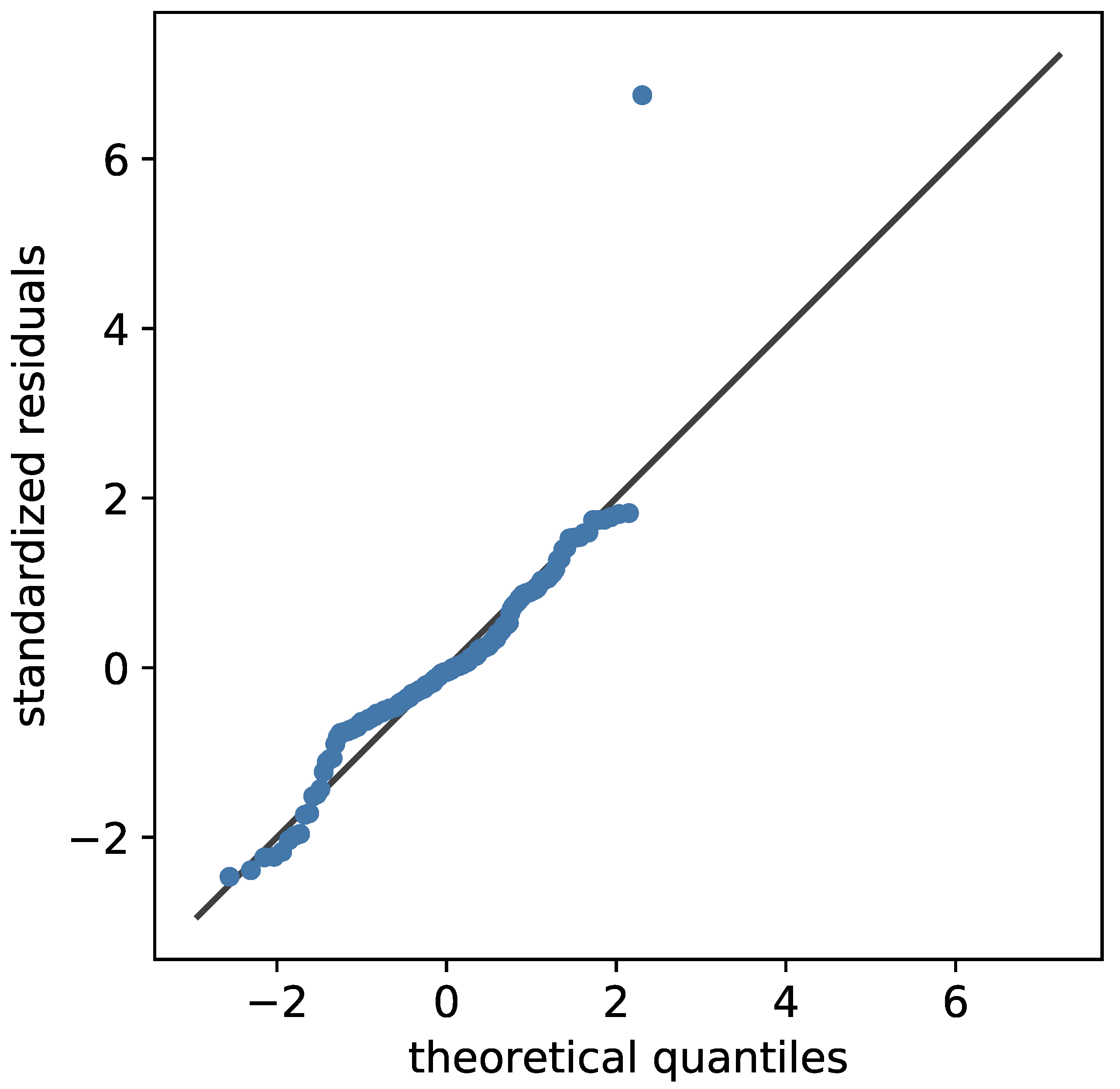
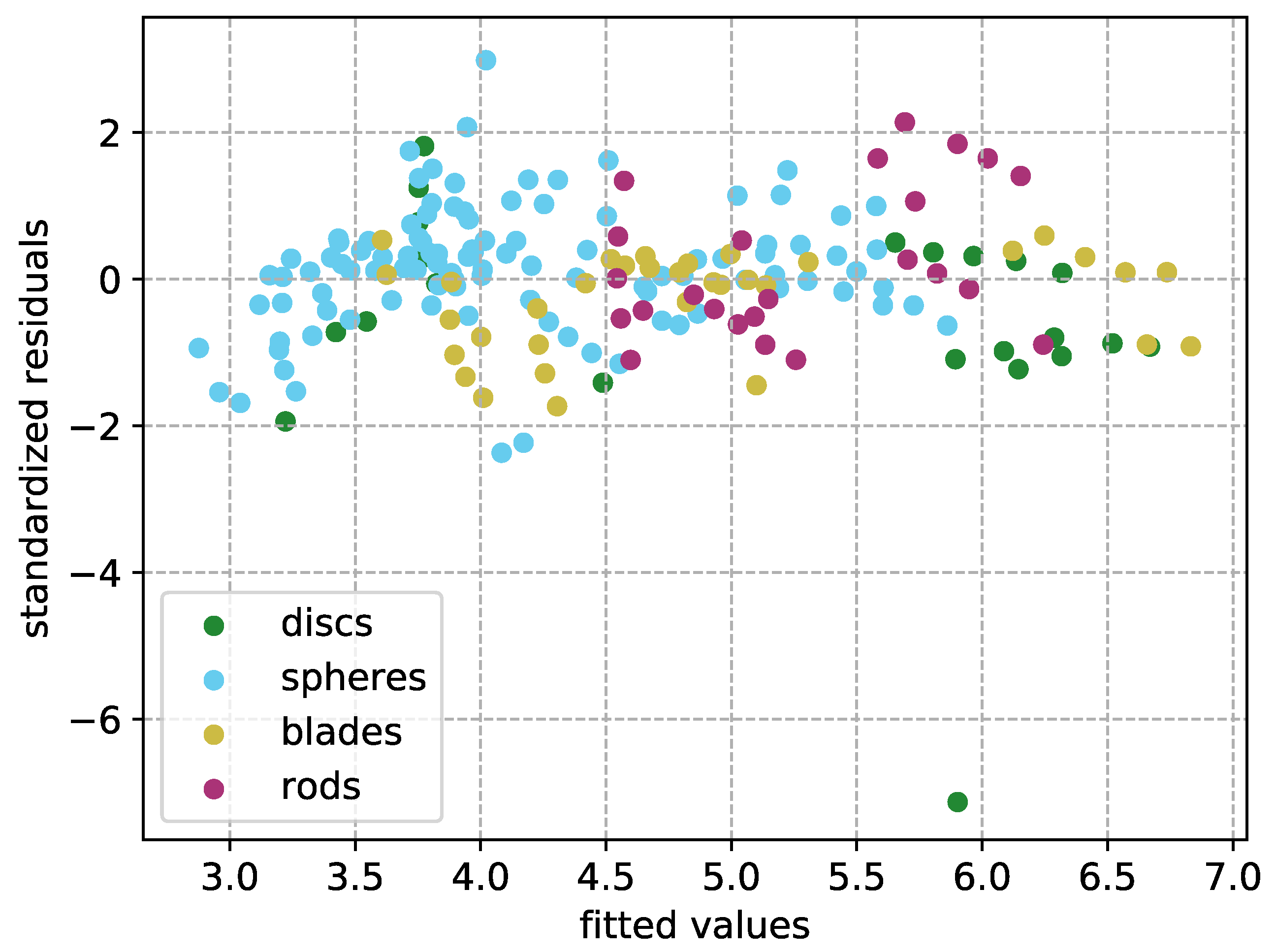
In addition, a polynomial regression regarding the terminal settling velocity was performed, for which only a few references were found in the literature. The found model yielded an adjusted coefficient of determination of $R_a^2=0.86$, relying on the particle density, sphericity, roundness and Hofmann shape entropy as the most relevant parameters. The mean deviation across training and test data was found to be $4.93\%$, which is approximately a fifth of the other models considered here. An error and outlier analysis also found good agreement between the simulated data and the model.

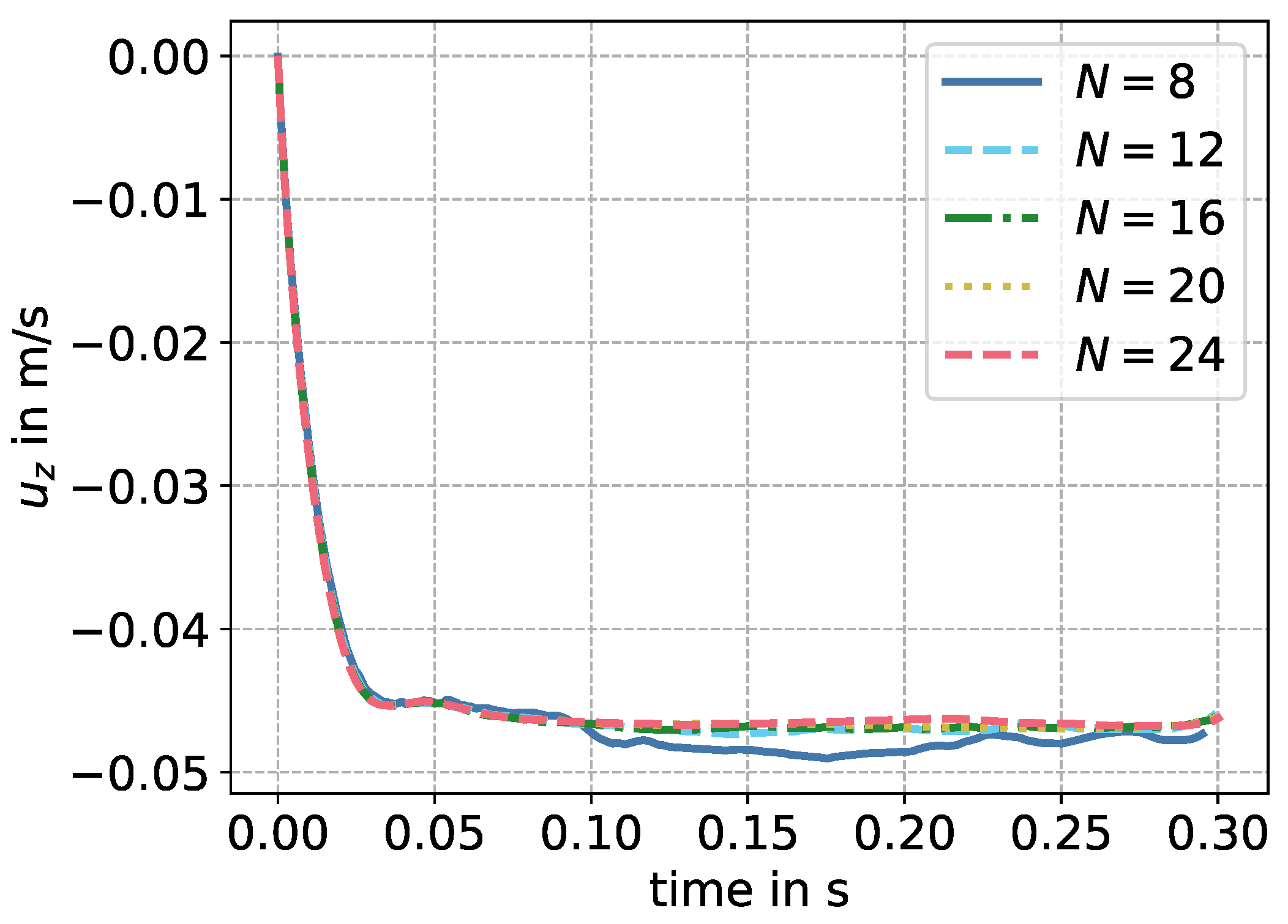
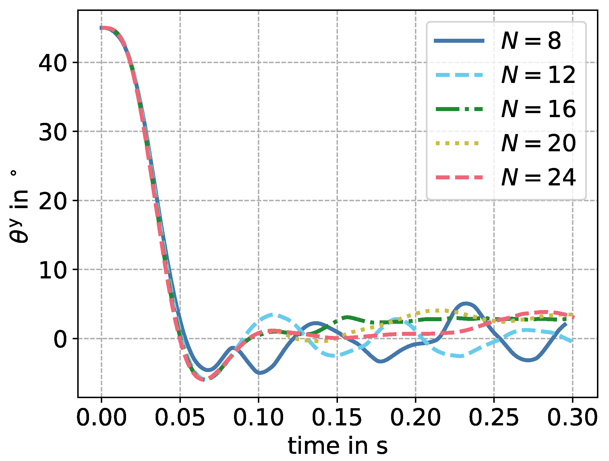
The considered particle collective was chosen to cover a wide range of equally distributed shape parameters to increase the significance of statistical results. Therefore, superellipsoids were used to describe the particles in numerical simulations. To focus on the influence of shape parameters, the particles are scaled to be equal in volume. Therefore, only a very limited range of Reynolds numbers in the intermediate regime was covered in this investigation. A first inspection showed that particles with a low value in flatness and ${\xi }_2=8$ did not reach their terminal settling velocity in the considered setup. To guarantee that particles reach the terminal settling velocity before reaching the bottom in future works, the domain is to move vertically along with the particle. This would also allow for a shorter domain, compared to the one in this study, thereby reducing the necessary computational effort.

It is, furthermore, possible to extend the described scheme to other setups, considering further effects like Brownian motion or additional external forces, and thereby obtain more specialized correlations.

References

1. Fu, X.; Huck, D.; Makein, L.; Armstrong, B.; Willen, U.; Freeman, T. Effect of particle shape and size on flow properties of lactose powders. Particuology 2012, 10, 203–208. [Google Scholar] [CrossRef]
2. Kashiwaya, K.; Noumachi, T.; Hiroyoshi, N.; Ito, M.; Tsunekawa, M. Effect of particle shape on hydrocyclone classification. Powder Technol. 2012, 226, 147–156. [Google Scholar] [CrossRef] [Green Version]
3. Champion, J.A.; Katare, Y.K.; Mitragotri, S. Particle shape: A new design parameter for micro- and nanoscale drug delivery carriers. J. Control. Release 2007, 121, 3–9. [Google Scholar] [CrossRef] [PubMed] [Green Version]
4. Waldschläger, K.; Schüttrumpf, H. Effects of Particle Properties on the Settling and Rise Velocities of Microplastics in Freshwater under Laboratory Conditions. Environ. Sci. Technol. 2019, 53, 1958–1966. [Google Scholar] [CrossRef] [PubMed]
5. Zingg, T. Beitrag zur Schotteranalyse. Ph.D. Thesis, ETH, Zürich, Switzerland, 1935. [Google Scholar]
6. Sneed, E.D.; Folk, R.L. Pebbles in the Lower Colorado River, Texas a Study in Particle Morphogenesis. J. Geol. 1958, 66, 114–150. [Google Scholar] [CrossRef]
7. ISO 9276-6:2008(E). Representation of Results of Particle Size Analysis—Part 6: Descriptive and Quantitative Representation of Particle Shape and Morphology; Standard; International Organization for Standardization: Geneva, Switzerland, 2008. [Google Scholar]
8. Hentschel, M.L.; Page, N.W. Selection of Descriptors for Particle Shape Characterization. Part. Part. Syst. Charact. 2003, 20, 25–38. [Google Scholar] [CrossRef]
9. Blott, S.J.; Pye, K. Particle shape: A review and new methods of characterization and classification. Sedimentology 2008, 55, 31–63. [Google Scholar] [CrossRef]
10. Allen, J.R.L. Chapter 5 Orientation of Particles During Sedimentation: Shape-Fabrics. In Sedimentary Structures Their Character and Physical Basis Volume I; Elsevier: Amsterdam, The Netherlands, 1982; Volume 30, pp. 179–235. [Google Scholar] [CrossRef]
11. Sheikh, M.Z.; Gustavsson, K.; Lopez, D.; Lévêque, E.; Mehlig, B.; Pumir, A.; Naso, A. Importance of fluid inertia for the orientation of spheroids settling in turbulent flow. J. Fluid Mech. 2020, 886. [Google Scholar] [CrossRef] [Green Version]
12. Bagheri, G.; Bonadonna, C. On the drag of freely falling non-spherical particles. Powder Technol. 2016, 301, 526–544. [Google Scholar] [CrossRef] [Green Version]
13. Komar, P.D.; Reimers, C.E. Grain Shape Effects on Settling Rates. J. Geol. 1978, 86, 193–209. [Google Scholar] [CrossRef]
14. Shao, B.; Liu, G.R.; Lin, T.; Xu, G.X.; Yan, X. Rotation and orientation of irregular particles in viscous fluids using the gradient smoothed method (GSM). Eng. Appl. Comput. Fluid Mech. 2017, 11, 557–575. [Google Scholar] [CrossRef]
15. Stokes, G.G. On the Effect of Internal Friction of Fluids on the Motion of Pendulums. Trans. Camb. Philos. Soc. 1851, 9, 8–106. [Google Scholar] [CrossRef] [Green Version]
16. Schiller, L.; Naumann, A. Über die grundlegenden Berechnungen bei der Schwerkraftaufbereitung. Z. Des Vereines Dtsch. Ingenieure 1933, 77, 318–320. [Google Scholar]
17. Clift, R.; Gauvin, W.H. Motion of entrained particles in gas streams. Can. J. Chem. Eng. 1971, 49, 439–448. [Google Scholar] [CrossRef]
18. McNown, J.S.; Malaika, J. Effects of particle shape on settling velocity at low Reynolds numbers. Trans. Am. Geophys. Union 1950, 31, 74. [Google Scholar] [CrossRef]
19. Sommerfeld, M.; Qadir, Z. Fluid dynamic forces acting on irregular shaped particles: Simulations by the Lattice–Boltzmann method. Int. J. Multiph. Flow 2018, 101, 212–222. [Google Scholar] [CrossRef]
20. Leith, D. Drag on Nonspherical Objects. Aerosol Sci. Technol. 1987, 6, 153–161. [Google Scholar] [CrossRef] [Green Version]
21. Ganser, G.H. A rational approach to drag prediction of spherical and nonspherical particles. Powder Technol. 1993, 77, 143–152. [Google Scholar] [CrossRef]
22. Loth, E. Drag of non-spherical solid particles of regular and irregular shape. Powder Technol. 2008, 182, 342–353. [Google Scholar] [CrossRef]
23. Hölzer, A.; Sommerfeld, M. New simple correlation formula for the drag coefficient of non-spherical particles. Powder Technol. 2008, 184, 361–365. [Google Scholar] [CrossRef]
24. Tran-Cong, S.; Gay, M.; Michaelides, E.E. Drag coefficients of irregularly shaped particles. Powder Technol. 2004, 139, 21–32. [Google Scholar] [CrossRef]
25. Dellino, P.; Mele, D.; Bonasia, R.; Braia, G.; La Volpe, L.; Sulpizio, R. The analysis of the influence of pumice shape on its terminal velocity. Geophys. Res. Lett. 2005, 32. [Google Scholar] [CrossRef]
26. Dioguardi, F.; Mele, D. A new shape dependent drag correlation formula for non-spherical rough particles. Experiments and results. Powder Technol. 2015, 277, 222–230. [Google Scholar] [CrossRef]
27. Hölzer, A.; Sommerfeld, M. Lattice Boltzmann simulations to determine drag, lift and torque acting on non-spherical particles. Comput. Fluids 2009, 38, 572–589. [Google Scholar] [CrossRef]
28. Haider, A.; Levenspiel, O. Drag coefficient and terminal velocity of spherical and nonspherical particles. Powder Technol. 1989, 58, 63–70. [Google Scholar] [CrossRef]
29. Henn, T.; Thäter, G.; Dörfler, W.; Nirschl, H.; Krause, M.J. Parallel dilute particulate flow simulations in the human nasal cavity. Comput. Fluids 2016, 124, 197–207. [Google Scholar] [CrossRef]
30. Trunk, R.; Henn, T.; Dörfler, W.; Nirschl, H.; Krause, M.J. Inertial dilute particulate fluid flow simulations with an Euler–Euler lattice Boltzmann method. J. Comput. Sci. 2016, 17, 438–445. [Google Scholar] [CrossRef]
31. Maier, M.L.; Milles, S.; Schuhmann, S.; Guthausen, G.; Nirschl, H.; Krause, M.J. Fluid flow simulations verified by measurements to investigate adsorption processes in a static mixer. Comput. Math. Appl. 2018, 76, 2744–2757. [Google Scholar] [CrossRef]
32. Trunk, R.; Marquardt, J.; Thäter, G.; Nirschl, H.; Krause, M.J. Towards the simulation of arbitrarily shaped 3D particles using a homogenised lattice Boltzmann method. Comput. Fluids 2018, 172, 621–631. [Google Scholar] [CrossRef]
33. Krause, M.J.; Klemens, F.; Henn, T.; Trunk, R.; Nirschl, H. Particle flow simulations with homogenised lattice Boltzmann methods. Particuology 2017, 34, 1–13. [Google Scholar] [CrossRef]
34. Trunk, R.; Weckerle, T.; Hafen, N.; Thäter, G.; Nirschl, H.; Krause, M.J. Revisiting the Homogenized Lattice Boltzmann Method with Applications on Particulate Flows. Computation 2021, 9, 11. [Google Scholar] [CrossRef]
35. Krause, M.J.; Kummerländer, A.; Avis, S.J.; Kusumaatmaja, H.; Dapelo, D.; Klemens, F.; Gaedtke, M.; Hafen, N.; Mink, A.; Trunk, R.; et al. OpenLB—Open source lattice Boltzmann code. Comput. Math. Appl. 2020. [Google Scholar] [CrossRef]
36. Krause, M.; Avis, S.; Kusumaatmaja, H.; Dapelo, D.; Gaedtke, M.; Hafen, N.; Haußmann, M.; Jeppener-Haltenhoff, J.; Kronberg, L.; Kummerländer, A.; et al. OpenLB Release 1.4: Open Source Lattice Boltzmann Code. Comput. Math. Appl. 2020. [Google Scholar] [CrossRef]
37. Yow, H.N.; Pitt, M.J.; Salman, A.D. Drag correlations for particles of regular shape. Adv. Powder Technol. 2005, 16, 363–372. [Google Scholar] [CrossRef]
38. Dey, S.; Ali, S.Z.; Padhi, E. Terminal fall velocity: The legacy of Stokes from the perspective of fluvial hydraulics. Proc. R. Soc. A Math. Phys. Eng. Sci. 2019, 475, 20190277. [Google Scholar] [CrossRef] [Green Version]
39. Bretl, C.; Trunk, R.; Nirschl, H.; Thäter, G.; Dorn, M.; Krause, M.J. Preliminary study of particle settling behaviour by shape parameters via lattice Boltzmann simulations. In High Performance Computing in Science and Engineering ’20; Nagel, W., Kröner, D., Resch, M., Eds.; Springer: Berlin/Heidelberg, Germany, 2020. [Google Scholar]
40. Wadell, H. Volume, Shape, and Roundness of Rock Particles. J. Geol. 1932, 40, 443–451. [Google Scholar] [CrossRef]
41. Krumbein, W.C. Measurement and Geological Significance of Shape and Roundness of Sedimentary Particles. SEPM J. Sediment. Res. 1941, 11. [Google Scholar] [CrossRef]
42. Hayakawa, Y.; Oguchi, T. Evaluation of gravel sphericity and roundness based on surface-area measurement with a laser scanner. Comput. Geosci. 2005, 31, 735–741. [Google Scholar] [CrossRef]
43. Dietrich, W.E. Settling velocity of natural particles. Water Resour. Res. 1982, 18, 1615–1626. [Google Scholar] [CrossRef]
44. Hofmann, H.J. Grain-shaped indices and isometric graphs. J. Sediment. Res. 1994, 64, 916–920. [Google Scholar] [CrossRef]
45. Le Roux, J.P. Application of the Hofmann shape entropy to determine the settling velocity of irregular, semi-ellipsoidal grains. Sediment. Geol. 2002, 149, 237–243. [Google Scholar] [CrossRef]
46. Le Roux, J. A Hydrodynamic Classification of Grain Shapes. J. Sediment. Res. 2004, 74, 135–143. [Google Scholar] [CrossRef]
47. Williams, J.R.; Pentland, A.P. Superquadrics and modal dynamics for discrete elements in interactive design. Eng. Comput. 1992, 9, 115–127. [Google Scholar] [CrossRef]
48. Barr, A.H. Superquadrics and Angle-Preserving Transformations. IEEE Comput. Graph. Appl. 1981, 1, 11–23. [Google Scholar] [CrossRef] [Green Version]
49. Wellmann, C.; Lillie, C.; Wriggers, P. A contact detection algorithm for superellipsoids based on the common-normal concept. Eng. Comput. 2008, 25, 432–442. [Google Scholar] [CrossRef] [Green Version]
50. Jaklič, A.; Leonardis, A.; Solina, F. Superquadrics and Their Geometric Properties. In Segmentation and Recovery of Superquadrics; Springer: Dordrecht, The Netherlands, 2000; pp. 13–39. [Google Scholar] [CrossRef]
51. Jaklič, A.; Solina, F. Moments of superellipsoids and their application to range image registration. IEEE Trans. Syst. Man Cybern. Part B (Cybern.) 2003, 33, 648–657. [Google Scholar] [CrossRef] [Green Version]
52. Bagheri, G.; Bonadonna, C. On the Drag of Freely Falling Non-Spherical Particles. Available online: https://arxiv.org/abs/1810.08787 (accessed on 25 March 2021).
53. Chrust, M.; Bouchet, G.; Dus̆ek, J. Numerical simulation of the dynamics of freely falling discs. Phys. Fluids 2013, 25, 044102. [Google Scholar] [CrossRef]
54. Seyed-Ahmadi, A.; Wachs, A. Dynamics and wakes of freely settling and rising cubes. Phys. Rev. Fluids 2018, 4. [Google Scholar] [CrossRef]
55. Rahmani, M.; Wachs, A. Free falling and rising of spherical and angular particles. Phys. Fluids 2014, 26, 083301. [Google Scholar] [CrossRef]
56. Kupershtokh, A.; Medvedev, D.; Karpov, D. On equations of state in a lattice Boltzmann method. Comput. Math. Appl. 2009, 58, 965–974. [Google Scholar] [CrossRef] [Green Version]
57. Wen, B.; Zhang, C.; Tu, Y.; Wang, C.; Fang, H. Galilean invariant fluid–solid interfacial dynamics in lattice Boltzmann simulations. J. Comput. Phys. 2014, 266, 161–170. [Google Scholar] [CrossRef] [Green Version]
58. Abraham, F.F. Functional Dependence of Drag Coefficient of a Sphere on Reynolds Number. Phys. Fluids 1970, 13, 2194. [Google Scholar] [CrossRef]
59. Krüger, T.; Kusumaatmaja, H.; Kuzmin, A.; Shardt, O.; Silva, G.; Viggen, E.M. The Lattice Boltzmann Method; Graduate Texts in Physics; Springer: Cham, Switzerland, 2017. [Google Scholar] [CrossRef]
60. Young, D.S. Handbook of Regression Methods; Chapman and Hall/CRC: Boca Raton, FL, USA, 2017. [Google Scholar] [CrossRef]
61. Pearson, K. VII. Mathematical contributions to the theory of evolution.—III. Regression, heredity, and panmixia. Philos. Trans. R. Soc. Lond. Ser. A Contain. Pap. A Math. Phys. Character 1896, 187, 253–318. [Google Scholar] [CrossRef] [Green Version]
62. Wisniewski, M. Applied Regression Analysis: A Research Tool. J. Oper. Res. Soc. 1990. [Google Scholar] [CrossRef]
63. Shannon, C.E. A Mathematical Theory of Communication. Bell Syst. Tech. J. 1948, 27, 379–423. [Google Scholar] [CrossRef] [Green Version]
64. Kraskov, A.; Stögbauer, H.; Grassberger, P. Estimating mutual information. Phys. Rev. E 2004, 69. [Google Scholar] [CrossRef] [Green Version]
65. Breiman, L. Random Forests. Mach. Learn. 2001, 45, 5–32. [Google Scholar] [CrossRef] [Green Version]
66. Horowitz, M.; Williamson, C.H.K. The effect of Reynolds number on the dynamics and wakes of freely rising and falling spheres. J. Fluid Mech. 2010, 651, 251–294. [Google Scholar] [CrossRef]
67. Szabó, T.; Domokos, G. A new classification system for pebble and crystal shapes based on static equilibrium points. Cent. Eur. Geol. 2010, 53, 1–19. [Google Scholar] [CrossRef] [Green Version]
68. Wilk, M.B.; Gnanadesikan, R. Probability plotting methods for the analysis for the analysis of data. Biometrika 1968, 55, 1–17. [Google Scholar] [CrossRef]
69. Thode, H.C. Testing For Normality; Taylor & Francis: Abingdon, UK, 2002. [Google Scholar] [CrossRef]
70. Anscombe, F.J.; Tukey, J.W. The Examination and Analysis of Residuals. Technometrics 1963, 5, 141–160. [Google Scholar] [CrossRef]
71. Cook, R.D. Detection of Influential Observation in Linear Regression. Technometrics 1977, 19, 15. [Google Scholar] [CrossRef]
Figure 1. Some examples of particle shapes considered via superellipsoids. Depicted (from left to right and top to bottom) are the particles with ID 5, 17, 28, 143, 166 and 200, according to Appendix A.
Computation 09 00040 g001
Figure 2. Initial configuration of the simulation.
Computation 09 00040 g002
Figure 3. Voxel representation of the particle with the shortest half-axis length of 9.1 × 10 5 m for N = 20 .
Computation 09 00040 g003
Figure 4. Coordinates of the center of mass of the particle, projected on a plane normal to the settling direction. Results printed for different grid spacings, for the particle with the shortest half-axis.
Computation 09 00040 g004
Figure 5. Plot of the angle for rotation around the y-axis over time during the settling. Results printed for different grid spacings, for the particle with the shortest half-axis.
Computation 09 00040 g005
Figure 6. Plot of the angle for rotation around the y-axis over time during the settling. Results printed for different grid spacings, for the particle with the longest half-axis.
Computation 09 00040 g006
Figure 7. Coordinates of the center of mass of the particle projected, on a plane normal to the settling direction. Results printed for different grid spacings, for the particle with the longest half-axis.
Computation 09 00040 g007
Figure 8. Dependency of the drag correction factor on elongation and flatness.
Computation 09 00040 g008
Figure 9. The particles considered in this study are plotted for a shape classification according to Zingg [5]. The four shape classes are 1: discs, 2: spheres, 3: blades and 4: rods.
Computation 09 00040 g009
Figure 10. The particles considered in this study are plotted for a shape classification according to Sneed and Folk [6]. They are also classified regarding the compactness, leading to the ten shape classes 1: compact, 2: compactly platy, 3: compactly bladed, 4: compactly elongated, 5: platy, 6: bladed, 7: elongated, 8: very platy, 9: very bladed and 10: very elongated.
Computation 09 00040 g010
Figure 11. The drag coefficient plotted against the Reynolds number, color with shape classification according to Zingg [5]. A spread is revealed, describable via the sphericity (marker style).
Computation 09 00040 g011
Figure 12. QQ-plot [68,69] of the standardized residuals against the theoretical quantiles of a normal distribution, revealing an approximately normal distributed error.
Computation 09 00040 g012
Figure 13. Tukey–Anscombe plot [70] showing the standardized residuals plotted against the fitted values, colored by shape classes according to Zingg [5].
Computation 09 00040 g013
Figure 14. QQ-plot [68,69] of the standardized residuals against the theoretical quantiles of a normal distribution, revealing a predominantly normal distributed error.
Computation 09 00040 g014
Figure 15. Tukey–Anscombe plot [70] showing the standardized residuals plotted against the fitted values, colored by shape classes according to Sneed and Folk [6].
Computation 09 00040 g015