Model and Analysis of Economic- and Risk-Based Objective Optimization Problem for Plant Location within Industrial Estates Using Epsilon-Constraint Algorithms

Abstract

In many countries, a number of industrial estates have been established to support the growth of the industrial sector, which is an essential strategy to drive economic growth. Planning for the location of industrial factories within an industrial estate, however, becomes complex, given the various types of industrial plants and the requirements of utilities to support operations within an industrial park. In this research, we model and analyze bi-objective optimization for locating plants within an industrial estate by considering economic- and risk-based cost objectives. Whereas economic objectives are associated with utility distances between plant locations, risk-based cost is a surrogate criterion derived from safety considerations. Next, risk-based data are further generated from Areal Locations of Hazardous Atmospheres (ALOHA), the hazard modeling program, and solutions to the bi-objective model are obtained from the Epsilon-constraint algorithm. Finally, the model is applied to a regional case study in a Thailand industrial estate, and the Pareto frontier is evaluated to demonstrate the trade-off between objectives.

1. Introduction

Recently, a number of countries have adopted various policies and expanded economical systems to support growth and globalization; these include technology promotion [1], tourism management [2], innovation expansion [3,4], and manufacturing technology [5]. One of the strategies to promote industrial expansion is the establishment of special economic zones to support the expansion of technological growth, facilitate industrial investment, and to attract foreign investment. The term “special economic zone” is used interchangeably with “industrial estate” and “industrial park” in the literature [6]. According to the United Nations Conference on Trade and Development (UNCTAD)’s 2019 World Investment Report [7], the recent trend of increasing industrial estates has been continuously reported across the globe. In particular, there were approximately 79 industrial estates in 1975, and since then the number of industrial estates has increased immensely; in 2018, there were a total of 5400 industrial estates. In particular, the expansion of industrial estates in special economic zones resulted in the total investment of more than 1200 billion dollars in the global economy in 2018. In Asia, particularly, industrial estates have been established in many regional areas with diverse aims; regions include China, India, Singapore, Malaysia, Cambodia, Vietnam, and Thailand [7,8,9]. In Thailand, in particular, there are industrial estates located currently in 16 provinces, and, since 2018, the Thai government has reported economic development plans to promote investment in 10 more provinces [9,10,11,12].

In this study, we develop a bi-objective, mixed-integer linear programming (MILP) model to analyze the location decisions of industrial factories within industrial estates. Initially, the cost to establish each industrial factory based on the installed piping system within the industrial estate layout is evaluated. Next, the safety surrogate is evaluated using the risk-based cost of the potential aftermath of an emergency event. The risk probability, in particular, is simulated from the chemical leakage scenario to estimate the diffusion radius of the explosion using Areal Locations of Hazardous Atmospheres (ALOHA), the hazard modeling program [13]. Thus, rather than merely implementing a mathematical modeling technique, the simulation technique is applied and integrated with the mathematical model [14,15,16]. Next, solutions to the bi-objective model are obtained from the Epsilon-constraint algorithm in which the trade-off between objectives is evaluated using the Pareto frontier. Finally, the model is applied to a regional case study within a Thailand industrial estate to verify the model functionalities.

This article consists of the following sections: Section 1 and Section 2 are the introduction and literature review, respectively; Section 3 presents the mathematical model; Section 4 discusses the case study and the results; a managerial insight is described in Section 5; and conclusions and directions for future research are provided in Section 6.

2. Literature Review

Production planning and control for factories has been gaining interest from various researchers for decades. Studies relevant to production planning typically focus on the development of models that assist in the planning of departments in a single production factory in which a single criterion of cost or distance consideration is employed. For example, researchers (e.g., [17,18,19]) have similarly proposed studies that aim to minimize the cost criterion in designing the industrial production process of a particular factory. The cost for minimizing piping distances for transporting raw materials and steam among departments in a factory is evaluated in these studies. In particular, the utility system is designed such that the shortest distance is ensured to optimize construction costs.

Another line of research involves considering the risk criterion in designing the production processes of a factory to improve safety conditions (e.g., [20,21,22]). For example, Yuan et al. [20] evaluated the industrial production process by taking into account the diffusion of toxic gas in determining the layout of different areas in a factory. The authors proposed a model for a layout assignment that could counter the impact of chemical spills. In addition, Medina-Herrera et al. [21] proposed a model for quantitative risk assessment of the factory layout to determine the position of the equipment and production processes, with an aim to reduce the cost from the risks associated with operators and equipment. In addition, Flores et al. [22] utilized the ALOHA software to assess the impact of fire and the explosion of flammable chemical storage and distribution vessels in chemical plants.

Additionally, both cost and risk criteria have been evaluated in a number of studies related to factory planning. For example, Rahman et al. [23] investigated the plant layout problem for an ammonia production plant by considering both the cost of production and the safety factor. In their study, the authors simulated the direction and spread of toxic gasses that could emanate from an explosion caused by excessive pressure in the main production process. Patsiatzis et al. [24] also analyzed the process layout of chemical plants to reduce the probability of accidents and optimize the installation cost. Furthermore, Jung et al. [25], Han et al. [26], and Ahumada et al. [27] similarly analyzed cost models associated with accidents using quantitative risk analysis and the cost of the production process in their study.

Few studies have examined the locational planning decisions for industrial estates [28,29,30,31]. The growth in industrial estates around the globe suggests that the planning and design of such estates based on strategic-level decision-making is required [28]. Recent researchers have thus proposed various strategic models for industrial estate planning. For example, Wang et al. [29] developed a model to optimize the layout of the industrial zone with the aim of minimizing cost and risk objectives using an experimental layout. The total cost was computed based on expenses incurred from the installation of the piping system, whereas the risk profile was determined based on the possibility of an explosion. According to the authors, proper arrangement of the industrial layout could reduce the cost of installing the piping system, as well as the impact of an accident. Moreover, Wattanasaeng and Ransikarbum [31] analyzed the relative locational efficiency of industrial estates to determine a candidate for special economic zones using a case study of Thailand provinces close to the country’s border. However, studies that aim to evaluate plant locational assignment for a particular industrial estate remain scarce. In addition, existing studies do not consider actual industrial estates featuring various types of industrial factories and lack trade-off analyses between conflicting criteria of interest.

In multiple objective programming, evaluated problems are concerned with mathematical optimization involving more than one objective function in which the objectives need to be optimized simultaneously or sequentially. In particular, in the literature, the Pareto or efficient frontier function has been used to illustrate the trade-offs among conflicts between multiple objectives [32]. Various techniques concerning exact and heuristic procedures have been proposed to analyze the trade-offs among these conflicting objectives, one of which is Epsilon-constraint programming [33]. The advantages of Epsilon-constraint programming include being able to obtain exact Pareto solutions, instead of approximated solutions, using a series of single-objective subproblems in which all but one objective is transformed into constraints. A number of researchers have applied the Epsilon-constraint algorithm in their studies. For example, Toro et al. [34] investigated the routing problem of transporting capacitors from a distribution center to high-demand areas. Epsilon-constraint programming was used to assess the trade-offs between cost and environmental objectives in the study. In addition, Abounacer et al. [35] proposed a model to aid humanitarian logistics operations in the aftermath of a disaster. The three objectives of minimum operation time, staff resources, and unsatisfied demand were analyzed using the Epsilon-constraint method and the Pareto frontier. Yu and Solvang [36] also used Epsilon-constraint programming to analyze the trade-offs between cost and risk objectives for waste management problems.

One of the most complex decisions in planning for industrial estates is designing the location of industrial factories in an industrial estate. This problem is further complicated by the various types of industrial plants and requirements of utilities needed to support the operations in industrial parks. Despite studies in this area being limited, existing studies were analyzed on the basis of planning for a particular factory or considering only a single objective. In particular, we highlight gaps in the existing literature and provide highlights for this study as follows:

• Plant location decision in industrial estate planning involves various stakeholders with often conflicting requirements. Thus, we develop the bi-objective, mixed-integer linear programming model based on economic and risk criteria to analyze the location decision of industrial factories in the industrial estate in this study.
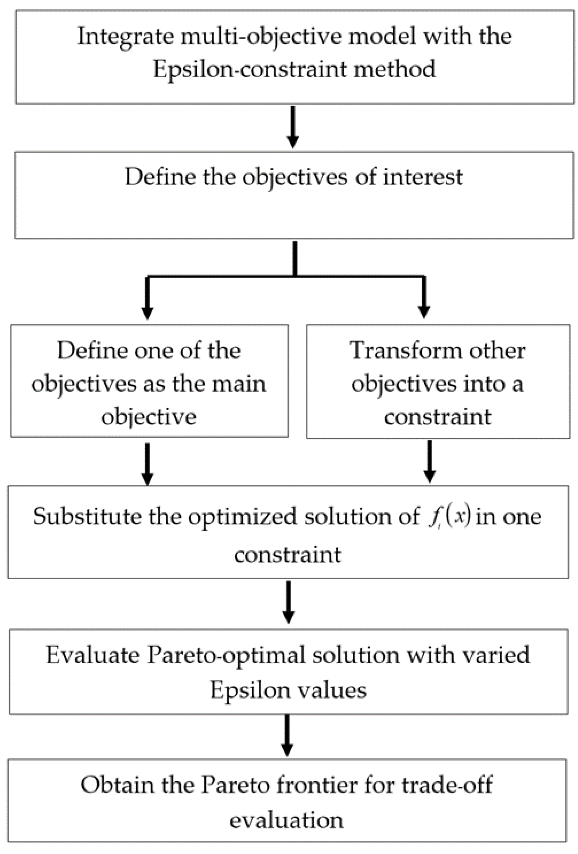
• Given the conflicting nature of bi-objective programming, the Epsilon-constraint method approach is further applied to analyze decision-makers’ preferences and to obtain the Pareto frontier in our analysis.
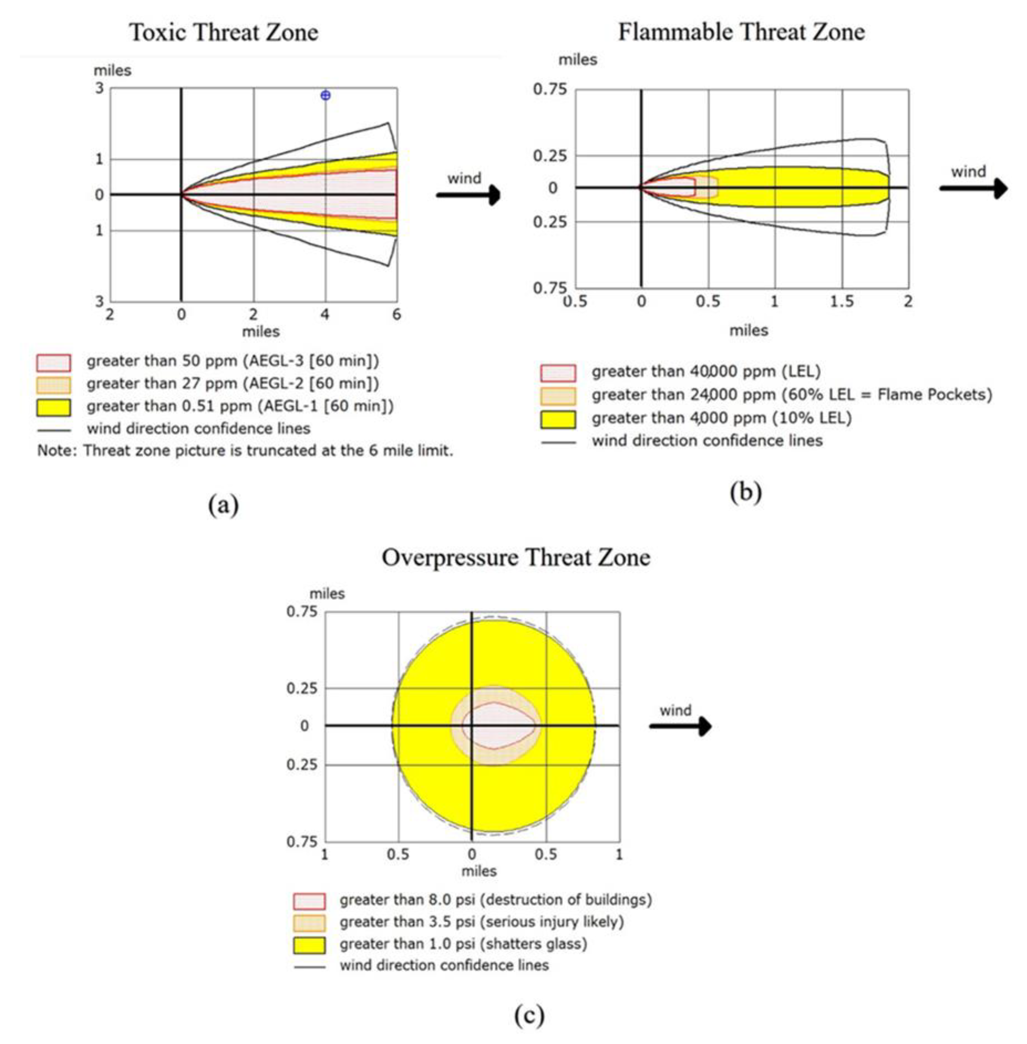
• In this study, both the bi-objective optimization technique and simulation procedure are used as an integrated tool in which the simulated risk profile obtained from the ALOHA program is used as an input for the developed optimization model in an integrated manner.
• Existing studies focus on developing the optimization model to design the production process of a single plant. In this study, our aim shifts to an analysis of the plant location problem comprising diverse factory classifications in the planned industrial estate.
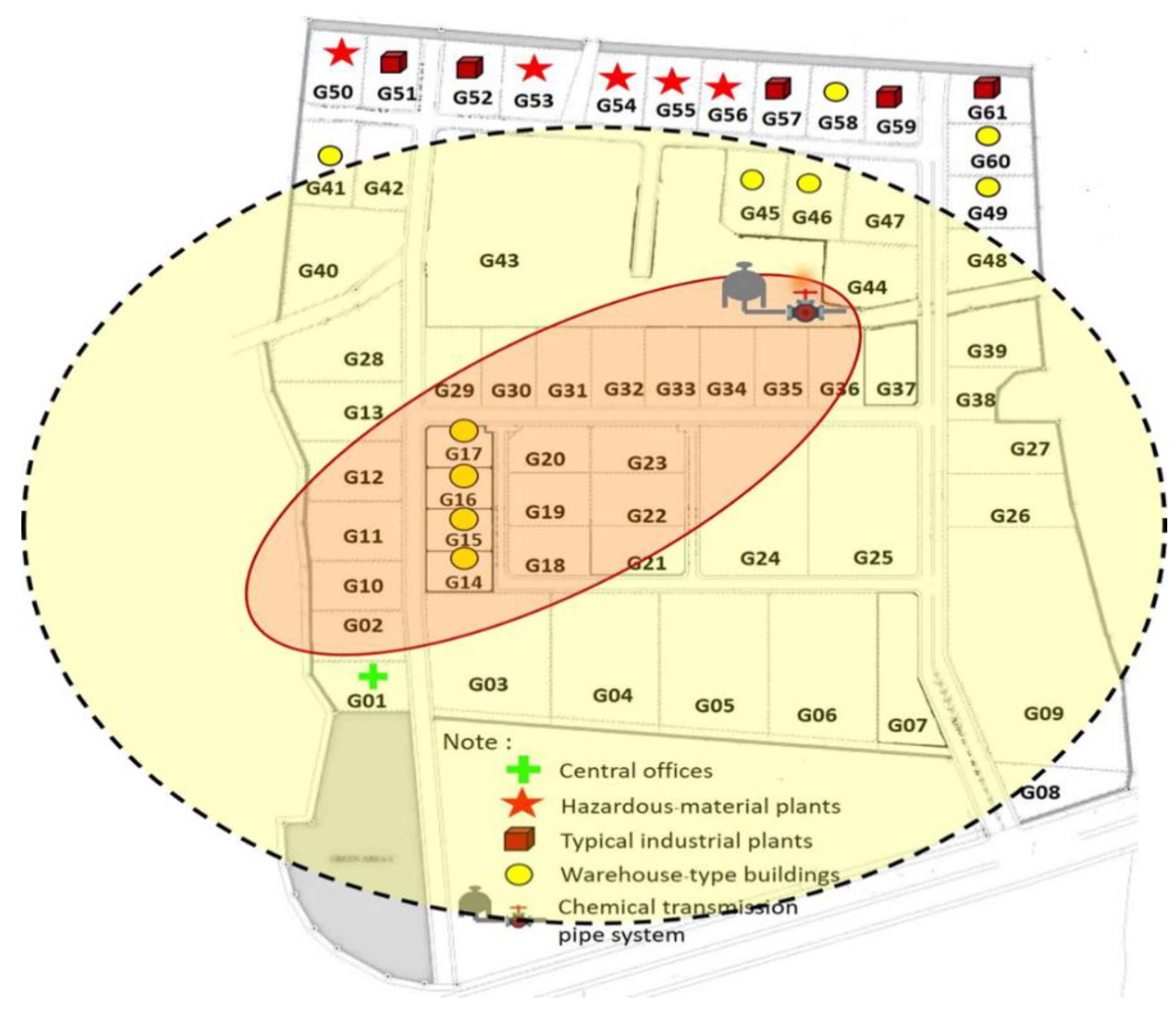
• The actual case study of the industrial estate located in Thailand is illustrated with actual data in this study. In addition, rather than applying the data to a general plant, we illustrate the model with diverse factory types in this study.

3. Methodology

We next discuss the proposed bi-objective mathematical optimization model for the plant location problem of a particular industrial estate. The developed model considers two objective functions based on the cost of assigning a plant location in an industrial estate and risk cost computed from the event of an emergency. In particular, the methodology is illustrated in Figure 1.

As its research scope, this paper presents a case study of an industrial estate located in the eastern region of Thailand. To illustrate how various plant types in the industrial estate affect the modeling complexity, we classify plant types into four subgroups. The first group is a hazardous-material factory working with highly flammable chemical substances; the second group is a warehouse-type building for storing raw materials and/or finished goods; the third group is a typical industrial factory without harmful substances; and the last group is a central office with supporting functions. Next, two objective functions reflecting the economic and safety criteria are evaluated, which are initially solved separately as a single-objective mathematical model to verify the model functionality and the layout planning. The economic criterion is then determined from the cost to establish plants in an industrial factory based on various distances between plant locations, and the safety criterion is evaluated with the ALOHA program using a risk profile based on an emergency. The risk probability is simulated based on a chemical leakage scenario to estimate the diffusion radius of the chemical explosion. The proposed model is then solved to achieve the optimal solution using A Mathematical Programming Language (AMPL) program, in which the Epsilon-constraint method is further used for the Pareto trade-off analysis, and to visualize how an improvement in one objective function jeopardizes the other objective function and vice versa.

3.1. Integrated Mathematical and Simulation Modeling

We next present the integrated mathematical model and simulation procedure implemented in this study. The general multi-objective problem modeled with the Epsilon-constraint method is illustrated in Equations (1)–(3). In particular, the multi-objective solution can be obtained from the Epsilon-constraint method by optimizing one particular objective of interest and transforming other objectives into a constraint set. Figure 2 illustrates the Epsilon-constraint procedure.

Minimize/Maximize Z: f_i(x)

(1)

Subject to: x ∈ X

(2)

$$f_i\left(x\right)\le {\epsilon }_j ; {\forall }_i\in \left\{1,\dots \dots ,k\right\} \backslash \left\{j\right\}$$

(3)

In addition, the hazard modeling program called ALOHA is used in this study. This program is capable of simulating the airborne spread of chemicals arising from an explosion. In this work, the ALOHA simulation program is used to simulate the spread of the hydrogen sulfide (H₂S) hypothetically used in the high-risk factories located in the industrial estate. Given the simulated results from the ALOHA program, the probability of risk associated with a chemical explosion that could affect diverse areas in the industrial estate is computed based on Equation (4) [29]. Then, the risk probability is used as input data for the proposed mathematical model. Figure 3 illustrates the explosion profile obtained from the ALOHA program.

$$Y= -15.6+1.93 In {\rho }^o$$

(4)

3.2. Assumptions

• The cost of the piping system is approximated based only on the distances between pairs of industrial plants. We assume that the same types of materials are transmitted through the industrial estate with no significant differences.
• The cost from risk is approximated based on an emergency situation that could hypothetically occur in the illustrated industrial estate; this cost is computed using the construction costs of buildings of various sizes. Thus, the cost from risk depends on the size of the area assigned to the industrial plant.
• The hazardous damage considered in this analysis is based on H₂S gas approximated via the ALOHA program; this damage hypothetically occurs in the location of the chemical transmission of the pipe system. Although a toxic threat, flammable threat, and overpressure threat were analyzed, only the overpressure threat is used in the analysis of damage in this study.
• Requirements related to the distance data between different plants were obtained from governmental regulations, as well as suggestions from concerned stakeholders of the presented industrial estate.
• The various building types in this study were classified into four categories: hazardous-material factory, warehouse-type building, typical industrial factory, and central office. Thus, the model complexity will depend on the number of building categories used in the analysis.

3.3. Mathematical Notation

Sets

• $G$: Set of grids in an industrial estate, indexed by k
• $P$: Set of all plants or buildings to be located, indexed by i
• $P^{TX}$: Set of hazardous-material plants to be located $P^{TX}$
• $P^{WH}$: Set of warehouse-type buildings to be located $\subseteq P$
• $P^{ID}$: Set of typical industrial plants to be located $\subseteq P$
• $P^{SZ}$: Set of central offices to be located $\subseteq P$

Parameters

Grid-related parameters

• $d_k^x$: The X coordinate of the $k^{th}$ grid from an office center (meter) $k\in G$
• $d_k^y$: The Y coordinate of the $k^{th}$ grid from an office center (meter) $k\in G$
• $r_k$: Risk probability for each $k^{th}$ grid $k\in G$
• $r_{rd}$: Rectilinear distance of the $k^{th}$ grid from an office center (meter) $k \in G$
• $c_k^{fc}$: Facility cost for each $k^{th}$ grid (Baht)
• $c_i^{up}$: Unit piping cost of the $i^{th}$ plant (Baht/meter) $i\in P$

Model-conversion parameters

• $m$: An arbitrary number for a fixed upper bound of distance for located plants

Minimum-separation parameters

• $d_{i,j}^{}$: Minimum separation distance between plants $i$ and $j$, $i,j \in D$
• $d_{i,j}^{TX\_SZ}$: Minimum separation distance between a hazardous-material plant $i \in P^{TX}$ and a central office $j \in P^{SZ}$
• $d_{i,j}^{TX\_ID}$: Minimum separation distance between a hazardous-material plant $i \in P^{TX}$ and a typical industrial plant $j \in P^{ID}$
• $d_{i,j}^{TX\_WH}$: Minimum separation distance between a hazardous-material plant $i \in P^{TX}$ and a warehouse-type building $j \in P^{WH}$
• $d_{i,j}^{WH\_SZ}$: Minimum separation distance between a warehouse-type building $i \in P^{WH}$ and a central office $j \in P^{SZ}$
• $d_{i,j}^{WH\_ID}$: Minimum separation distance between a warehouse-type building $i \in P^{WH}$ and a typical industrial plant $i \in P^{ID}$
• $d_{i,j}^{ID\_SZ}$: Minimum separation distance between a typical industrial plant $i \in P^{ID}$ and a central office $j \in P^{SZ}$

Maximum-separation parameters

• $m_{i,j}^{TX\_SZ\_1, 2, 3, 4}$: Maximum separation distance between a hazardous-material plant $i \in P^{TX}$ and a central office $j \in P^{SZ}$ with four respective parameters
• $m_{i,j}^{TX\_WH\_1, 2,3,4}$: Maximum separation distance between a hazardous-material plant $i \in P^{TX}$ and a warehouse-type building $j \in P^{WH}$ with four respective parameters
• $m_{i,j}^{TX\_ID\_1,2,3,4}$: Maximum separation distance between a hazardous-material plant $i \in P^{TX}$ and a typical industrial plant $j \in P^{ID}$ with four respective parameters
• $m_{i,j}^{WH\_SZ\_1,2,3,4}$: Maximum separation distance between a warehouse-type building $i \in P^{WH}$ and a central office $j \in P^{SZ}$ with four respective parameters
• $m_{i,j}^{WH\_ID\_1,2,3,4}$: Maximum separation distance between a warehouse-type building $i \in P^{WH}$ and a typical industrial plant $j \in P^{ID}$ with four respective parameters
• $m_{i,j}^{ID\_SZ\_1,2,3,4}$: Maximum separation distance between a typical industrial plant $i \in P^{ID}$ and a central office $j \in P^{SZ}$ with four respective parameters

Decision variables

• $B_{i,k}$: A variable to assign a plant $i\in P$ to grid $k \in G$, binary {0, 1}
• $X_i$: The X coordinate of located plant $i\in P$
• $Y_i$: The Y coordinate of located plant $i\in P$

Auxiliary variables

• $SE{P}_{i,j}^{TX\_SZ\_1,2,3,4}$: Supporting variable for minimum separation distance between a hazardous-material plant $i \in P^{TX}$ and a central office $j \in P^{SZ}$ with four respective variables, binary {0, 1}
• $SE{P}_{i,j}^{TX\_WH\_1,2,3,4}$: Supporting variable for minimum separation distance between a hazardous-material plant $i \in P^{TX}$ and a warehouse-type building $j \in P^{WH}$ with four respective variables, binary {0, 1}
• $SE{P}_{i,j}^{TX\_ID\_1,2,3,4}$: Supporting variable for minimum separation distance between a hazardous-material plant $i \in P^{TX}$ and a typical industrial plant $j \in P^{ID}$ with four respective variables, binary {0, 1}
• $SE{P}_{i,j}^{WH\_SZ\_1,2,3,4}$: Supporting variable for minimum separation distance between a warehouse-type building $i \in P^{WH}$ and a central office $j \in P^{SZ}$ with four respective variables, binary {0, 1}
• $SE{P}_{i,j}^{WH\_ID\_1,2,3,4}$: Supporting variable for minimum separation distance between a warehouse-type building $i \in P^{WH}$ and a typical industrial plant $j \in P^{ID}$ with four respective variables, binary {0, 1}
• $SE{P}_{i,j}^{ID\_SZ\_1,2,3,4}$: Supporting variable for minimum separation distance between a typical industrial plant $i \in P^{ID}$ and a central office $j \in P^{SZ}$ with four respective variables, binary {0, 1}

3.4. Objective Functions

The objective functions are provided based on two different perspectives for the developed bi-objective optimization model. In particular, the first objective function represents the economic criterion, in which the total piping cost associated with the installed pipeline system between all pairs of buildings in the industrial estate can be computed as shown in Equation (5). The $r_{rd}$ parameter, in particular, is the rectilinear distance computed from the distances between the X and Y coordinates of any assigned plants and an office center. In addition, the $B_{i,k}$ variable represents the assignment of the plant.

$$\mathrm{Minimize} Z1:{\displaystyle \sum _{i\in P}^{}{\displaystyle \sum _{k\in K }^{}}}\left\{c_i^{up}{r}_{rd}\right\}{B}_{i,k}$$

(5)

Next, the second objective function represents the safety consideration in which the associated risk probability ($r_k$) from an emergency situation that hypothetically occurs at the industrial estate is to be minimized. That is, the total risk cost ($c_k^{fc}$), derived from the ALOHA software, is computed from the risk probability assigned to each area of the industrial estate. Equation (6), in particular, presents the formula of this objective function.

$$\mathrm{Minimize} Z2:{\displaystyle \sum _{i\in P}^{}{\displaystyle \sum _{k\in K }^{} \left\{r_k^{}{c}_k^{fc}\right\}}} B_{i,k}$$

(6)

3.5. Constraint Sets

We next discuss the requirements associated with regulations and constraints for assigning different factory types in various locations in an illustrated industrial estate. In particular, the relevant constraints sets for non-overlapping restriction, distance computation, minimum separation requirement, maximum separation requirement, and house-keeping are illustrated below.

3.5.1. Non-Overlapping Constraint Set

Initially, the non-overlapping constraint sets in Equations (7) and (8) are used to ensure that established plants in the industrial estate do not overlap, where the $B_{i,k}$ variable represents the assignment of the plant on a grid. In particular, whereas each assigned plant must be located in the industrial estate layout (Equation (7)), each grid in the industrial estate is not necessarily required to have a plant assigned (Equation (8)).

$${\displaystyle \sum _{k\in K}{B}_{i,k} = 1 ; \forall i\in P}$$

(7)

$${\displaystyle \sum _{i\in P}{B}_{i,k} \le 1 ;\forall k\in G}$$

(8)

3.5.2. Distance-Related Constraint Set

In addition, the distance between any grids of the industrial estate’s layout can be rectilinearly computed, as presented in Equations (9)–(12). That is, given the assigned plants on respective grids, the distance along the X and Y axes to the location of the assigned plants can be computed as illustrated below, where $d_k^x$ and $d_k^y$ are the X and Y coordinates of the $k^{th}$ grid from an office center, respectively.

$$-m\left(1-B_{i,k}\right) \le \left(d_k^x-X_i\right) ; \forall i\in P,\forall k\in G$$

(9)

$$\left(d_k^x - X_i\right) \le m \left(1-B_{i,k}\right) ; \forall i\in P,\forall k\in G$$

(10)

$$-m\left(1-B_{i,k}\right) \le \left(d_k^x-X_i\right) ; \forall i\in P,\forall k\in G$$

(11)

$$\left(d_k^y - Y_i\right) \le m \left(1-B_{i,k}\right) ; \forall i\in P,\forall k\in G$$

(12)

3.5.3. Separation-Distance Constraint Set for the Minimum Condition

We next discuss the minimum separation requirement. That is, the following sets of constraints are to ensure the least distance for any pairs of assigned plants in the industrial estate, which implies associated safety requirements to reduce damage in the event of an emergency [25]. Although the absolute value in Equation (13) to compute the distance between any pairs of industrial plants ($d_{i,j}$) is in non-linear form, this equation can be subsequently transformed to a linear form.

$$\left|X_i-X_j\right|+\left|Y_i-Y_j\right|\ge d_{i,j}$$

(13)

In particular, we illustrate respective linear constraint sets between a hazardous-material plant and a central office, as shown in Equations (14)–(18):

$$\left(X_i-X_j\right)+\left(Y_i-Y_j\right) \ge d_{i,j}^{TX\_SZ}*SE{P}_{i,j}^{TX\_SZ\_1} -\left(m*\left(1-SE{P}_{i,j}^{TX\_SZ\_1}\right)\right) ; \forall i\in P^{TX}, \forall j\in P^{SZ}$$

(14)

$$\left(X_i-X_j\right)-\left(Y_i-Y_j\right)\ge d_{i,j}^{TX\_SZ}*SE{P}_{i,j}^{TX\_SZ\_2} -\left(m*\left(1-SE{P}_{i,j}^{TX\_SZ\_2}\right)\right) ; \forall i\in P^{TX}, \forall j\in P^{SZ}$$

(15)

$$-\left(X_i-X_j\right)+\left(Y_i-Y_j\right) \ge d_{i,j}^{TX\_SZ}*SE{P}_{i,j}^{TX\_SZ\_3} -\left(m*\left(1-SE{P}_{i,j}^{TX\_SZ\_3}\right)\right) ; \forall i\in P^{TX}, \forall j\in P^{SZ}$$

(16)

$$-\left(X_i-X_j\right)+\left(Y_i-Y_j\right) \ge d_{i,j}^{TX\_SZ}*SE{P}_{i,j}^{TX\_SZ\_4} -\left(m*\left(1-SE{P}_{i,j}^{TX\_SZ\_4}\right)\right) ; \forall i\in P^{TX}, \forall j\in P^{SZ}$$

(17)

$$SE{P}^{TX\_SZ\_1}+SE{P}^{TX\_SZ\_2}+SE{P}^{TX\_SZ\_3}+SE{P}^{TX\_SZ\_4} \ge 1$$

(18)

The sets of constraints for the minimum-distance separation between the pair of a hazardous-material plant and a warehouse-type building are shown in Equations (19)–(23):

$$\left(X_i-X_j\right)+\left(Y_i-Y_j\right) \ge d_{i,j}^{TX\_WH}*SE{P}_{i,j}^{TX\_WH\_1} -\left(m*\left(1-SE{P}_{i,j}^{TX\_WH\_1}\right)\right) ; \forall i\in P^{TX}, \forall j\in P^{WH}$$

(19)

$$\left(X_i-X_j\right)-\left(Y_i-Y_j\right)\ge d_{i,j}^{TX\_WH}*SE{P}_{i,j}^{TX\_WH\_2} -\left(m*\left(1-SE{P}_{i,j}^{TX\_WH\_2}\right)\right) ; \forall i\in P^{TX}, \forall j\in P^{WH}$$

(20)

$$-\left(X_i-X_j\right)+\left(Y_i-Y_j\right) \ge d_{i,j}^{TX\_WH}*SE{P}_{i,j}^{TX\_WH\_3} -\left(m*\left(1-SE{P}_{i,j}^{TX\_WH\_3}\right)\right) ; \forall i\in P^{TX}, \forall j\in P^{WH}$$

(21)

$$-\left(X_i-X_j\right)+\left(Y_i-Y_j\right) \ge d_{i,j}^{TX\_WH}*SE{P}_{i,j}^{TX\_WH\_4} -\left(m*\left(1-SE{P}_{i,j}^{TX\_WH\_4}\right)\right) ; \forall i\in P^{TX}, \forall j\in P^{WH}$$

(22)

$$SE{P}^{TX\_WH\_1}+SE{P}^{TX\_WH\_2}+SE{P}^{TX\_WH\_3}+SE{P}^{TX\_WH\_4} \ge 1$$

(23)

The sets of constraints for the minimum-distance separation for the pair of a hazardous-material plant and a typical industrial plant are shown in Equations (24)–(28):

$$\left(X_i-X_j\right)+\left(Y_i-Y_j\right) \ge d_{i,j}^{TX\_ID}*SE{P}_{i,j}^{TX\_ID\_1} -\left(m*\left(1-SE{P}_{i,j}^{TX\_ID\_1}\right)\right) ; \forall i\in P^{TX}, \forall j\in P^{ID}$$

(24)

$$\left(X_i-X_j\right)-\left(Y_i-Y_j\right)\ge d_{i,j}^{TX\_ID}*SE{P}_{i,j}^{TX\_ID\_2} -\left(m*\left(1-SE{P}_{i,j}^{TX\_ID\_2}\right)\right) ; \forall i\in P^{TX}, \forall j\in P^{ID}$$

(25)

$$-\left(X_i-X_j\right)+\left(Y_i-Y_j\right) \ge d_{i,j}^{TX\_ID}*SE{P}_{i,j}^{TX\_ID\_3} -\left(m*\left(1-SE{P}_{i,j}^{TX\_ID\_3}\right)\right) ; \forall i\in P^{TX}, \forall j\in P^{ID}$$

(26)

$$-\left(X_i-X_j\right)+\left(Y_i-Y_j\right) \ge d_{i,j}^{TX\_ID}*SE{P}_{i,j}^{TX\_ID\_4} -\left(m*\left(1-SE{P}_{i,j}^{TX\_ID\_4}\right)\right) ; \forall i\in P^{TX}, \forall j\in P^{ID}$$

(27)

$$SE{P}^{TX\_ID\_1}+SE{P}^{TX\_ID\_2}+SE{P}^{TX\_ID\_3}+SE{P}^{TX\_ID\_4} \ge 1$$

(28)

The sets of constraints for the minimum-distance separation for the pair of a warehouse-type building and a typical industrial plant are shown in Equations (29)–(33):

$$\left(X_i-X_j\right)+\left(Y_i-Y_j\right) \ge d_{i,j}^{WH\_ID}*SE{P}_{i,j}^{WH\_ID\_1} -\left(m*\left(1-SE{P}_{i,j}^{WH\_ID\_1}\right)\right) ; \forall i\in P^{WH}, \forall j\in P^{ID}$$

(29)

$$\left(X_i-X_j\right)-\left(Y_i-Y_j\right)\ge d_{i,j}^{WH\_ID}*SE{P}_{i,j}^{WH\_ID\_2} -\left(m*\left(1-SE{P}_{i,j}^{WH\_ID\_2}\right)\right) ; \forall i\in P^{WH}, \forall j\in P^{ID}$$

(30)

$$-\left(X_i-X_j\right)+\left(Y_i-Y_j\right) \ge d_{i,j}^{WH\_ID}*SE{P}_{i,j}^{WH\_ID\_3} -\left(m*\left(1-SE{P}_{i,j}^{WH\_ID\_3}\right)\right) ; \forall i\in P^{WH}, \forall j\in P^{ID}$$

(31)

$$-\left(X_i-X_j\right)+\left(Y_i-Y_j\right) \ge d_{i,j}^{WH\_ID}*SE{P}_{i,j}^{WH\_ID\_4} -\left(m*\left(1-SE{P}_{i,j}^{WH\_ID\_4}\right)\right) ; \forall i\in P^{WH}, \forall j\in P^{ID}$$

(32)

$$SE{P}^{WH\_ID\_1}+SE{P}^{WH\_ID\_2}+SE{P}^{WH\_ID\_3}+SE{P}^{WH\_ID\_4} \ge 1$$

(33)

The sets of constraints for the minimum-distance separation for the pair of a warehouse-type building and a central office are shown in Equations (34)–(38):

$$\left(X_i-X_j\right)+\left(Y_i-Y_j\right) \ge d_{i,j}^{WH\_SZ}*SE{P}_{i,j}^{WH\_SZ\_1} -\left(m*\left(1-SE{P}_{i,j}^{WH\_SZ\_1}\right)\right) ; \forall i\in P^{WH}, \forall j\in P^{SZ}$$

(34)

$$\left(X_i-X_j\right)-\left(Y_i-Y_j\right)\ge d_{i,j}^{WH\_SZ}*SE{P}_{i,j}^{WH\_SZ\_2} -\left(m*\left(1-SE{P}_{i,j}^{WH\_SZ\_2}\right)\right) ; \forall i\in P^{WH}, \forall j\in P^{SZ}$$

(35)

$$-\left(X_i-X_j\right)+\left(Y_i-Y_j\right) \ge d_{i,j}^{WH\_SZ}*SE{P}_{i,j}^{WH\_SZ\_3} -\left(m*\left(1-SE{P}_{i,j}^{WH\_SZ\_3}\right)\right) ; \forall i\in P^{WH}, \forall j\in P^{SZ}$$

(36)

$$-\left(X_i-X_j\right)+\left(Y_i-Y_j\right) \ge d_{i,j}^{WH\_SZ}*SE{P}_{i,j}^{WH\_SZ\_4} -\left(m*\left(1-SE{P}_{i,j}^{WH\_SZ\_4}\right)\right) ; \forall i\in P^{WH}, \forall j\in P^{SZ}$$

(37)

$$SE{P}^{WH\_SZ\_1}+SE{P}^{WH\_SZ\_2}+SE{P}^{WH\_SZ\_3}+SE{P}^{WH\_SZ\_4} \ge 1$$

(38)

Finally, the sets of constraints for the minimum-distance separation for the pair of a typical industrial plant and a central office are shown in Equations (39)–(43):

$$\left(X_i-X_j\right)+\left(Y_i-Y_j\right) \ge d_{i,j}^{ID\_SZ}*SE{P}_{i,j}^{ID\_SZ\_1} -\left(m*\left(1-SE{P}_{i,j}^{ID\_SZ\_1}\right)\right) ; \forall i\in P^{ID}, \forall j\in P^{SZ}$$

(39)

$$\left(X_i-X_j\right)-\left(Y_i-Y_j\right)\ge d_{i,j}^{ID\_SZ}*SE{P}_{i,j}^{ID\_SZ\_2} -\left(m*\left(1-SE{P}_{i,j}^{ID\_SZ\_2}\right)\right) ; \forall i\in P^{ID}, \forall j\in P^{SZ}$$

(40)

$$-\left(X_i-X_j\right)+\left(Y_i-Y_j\right) \ge d_{i,j}^{ID\_SZ}*SE{P}_{i,j}^{ID\_SZ\_3} -\left(m*\left(1-SE{P}_{i,j}^{ID\_SZ\_3}\right)\right) ; \forall i\in P^{ID}, \forall j\in P^{SZ}$$

(41)

$$-\left(X_i-X_j\right)+\left(Y_i-Y_j\right) \ge d_{i,j}^{ID\_SZ}*SE{P}_{i,j}^{ID\_SZ\_4} -\left(m*\left(1-SE{P}_{i,j}^{ID\_SZ\_4}\right)\right) ; \forall i\in P^{ID}, \forall j\in P^{SZ}$$

(42)

$$SE{P}^{ID\_SZ\_1}+SE{P}^{ID\_SZ\_2}+SE{P}^{ID\_SZ\_3}+SE{P}^{ID\_SZ\_4} \ge 1$$

(43)

3.5.4. Separation-Distance Constraint Set for the Maximum Condition

Similarly, the next sets of constraints ensure that associated plants located in the industrial estate are not established too remotely following the regulation and requirements of the industrial estate, as shown in Equation (44) where $m_{ij}$ is the maximum separation distance between any pairs of industrial plants. The non-linear separation-distance constraint set ensuring the maximum condition is linearly transformed for each pair of building types is as follows:

$$\left|X_i-X_j\right| + \left|Y_i-Y_j\right| \le m_{ij}$$

(44)

The sets of constraints for the maximum-distance separation for the pair of a hazardous-material plant and a central office are shown in Equations (45)–(49):

$$\left(X_i-X_j\right)+\left(Y_i-Y_j\right)\le m_{i,j}^{TX\_SZ\_1} ; \forall i\in P^{TX},\forall j\in P^{SZ}$$

(45)

$$\left(X_i-X_j\right)-\left(Y_i+Y_j\right)\le m_{i,j}^{TX\_SZ\_2} ; \forall i\in P^{TX},\forall j\in P^{SZ}$$

(46)

$$-\left(X_i+X_j\right)+\left(Y_i-Y_j\right)\le m_{i,j}^{TX\_SZ\_3} ; \forall i\in P^{TX},\forall j\in P^{SZ}$$

(47)

$$-\left(X_i+X_j\right)-\left(Y_i+Y_j\right)\le m_{i,j}^{TX\_SZ\_4} ; \forall i\in P^{TX},\forall j\in P^{SZ}$$

(48)

$$m_{i,j}^{TX\_SZ\_1} + m_{i,j}^{TX\_SZ\_2} + m_{i,j}^{TX\_SZ\_3} + m_{i,j}^{TX\_SZ\_4} \ge 1$$

(49)

The sets of constraints for the maximum-distance separation for the pair of a hazardous-material plant and a warehouse-type building are shown in Equations (50)–(54):

$$\left(X_i-X_j\right)+\left(Y_i-Y_j\right)\le m_{i,j}^{TX\_WH\_1} ; \forall i\in P^{TX},\forall j\in P^{WH}$$

(50)

$$\left(X_i-X_j\right)-\left(Y_i+Y_j\right)\le m_{i,j}^{TX\_WH\_2} ; \forall i\in P^{TX},\forall j\in P^{WH}$$

(51)

$$-\left(X_i+X_j\right)+\left(Y_i-Y_j\right)\le m_{i,j}^{TX\_WH\_3} ; \forall i\in P^{TX},\forall j\in P^{WH}$$

(52)

$$-\left(X_i+X_j\right)-\left(Y_i+Y_j\right)\le m_{i,j}^{TX\_WH\_4} ; \forall i\in P^{TX},\forall j\in P^{WH}$$

(53)

$$m_{i,j}^{TX\_WH\_1} + m_{i,j}^{TX\_WH\_2} + m_{i,j}^{TX\_WH\_3} + m_{i,j}^{TX\_WH\_4} \ge 1$$

(54)

The sets of constraints for the maximum-distance separation for the pair of a hazardous-material plant and a typical industrial plant are shown in Equations (55)–(59):

$$\left(X_i-X_j\right)+\left(Y_i-Y_j\right)\le m_{i,j}^{TX\_ID\_1} ; \forall i\in P^{TX},\forall j\in P^{ID}$$

(55)

$$\left(X_i-X_j\right)-\left(Y_i+Y_j\right)\le m_{i,j}^{TX\_ID\_2} ; \forall i\in P^{TX},\forall j\in P^{ID}$$

(56)

$$-\left(X_i+X_j\right)+\left(Y_i-Y_j\right)\le m_{i,j}^{TX\_ID\_3} ; \forall i\in P^{TX},\forall j\in P^{ID}$$

(57)

$$-\left(X_i+X_j\right)-\left(Y_i+Y_j\right)\le m_{i,j}^{TX\_ID\_4} ; \forall i\in P^{TX},\forall j\in P^{ID}$$

(58)

$$m_{i,j}^{TX\_ID\_1} + m_{i,j}^{TX\_ID\_2} + m_{i,j}^{TX\_ID\_3} + m_{i,j}^{TX\_ID\_4} \ge 1$$

(59)

The sets of constraints for the maximum-distance separation for the pair of a warehouse-type building and a central office are shown in Equations (60)–(64):

$$\left(X_i-X_j\right)+\left(Y_i-Y_j\right)\le m_{i,j}^{WH\_SZ\_1} ; \forall i\in P^{WH},\forall j\in P^{SZ}$$

(60)

$$\left(X_i-X_j\right)-\left(Y_i+Y_j\right)\le m_{i,j}^{WH\_SZ\_2} ; \forall i\in P^{WH},\forall j\in P^{SZ}$$

(61)

$$-\left(X_i+X_j\right)+\left(Y_i-Y_j\right)\le m_{i,j}^{WH\_SZ\_3} ; \forall i\in P^{WH},\forall j\in P^{SZ}$$

(62)

$$-\left(X_i+X_j\right)-\left(Y_i+Y_j\right)\le m_{i,j}^{WH\_SZ\_4} ; \forall i\in P^{WH},\forall j\in P^{SZ}$$

(63)

$$m_{i,j}^{WH\_SZ\_1} + m_{i,j}^{WH\_SZ\_2} + m_{i,j}^{WH\_SZ\_3} + m_{i,j}^{WH\_SZ\_4} \ge 1$$

(64)

The sets of constraints for the maximum-distance separation for the pair of a warehouse-type building and a typical industrial plant are shown in Equations (65)–(69):

$$\left(X_i-X_j\right)+\left(Y_i-Y_j\right)\le m_{i,j}^{WH\_ID\_1} ; \forall i\in P^{WH},\forall j\in P^{ID}$$

(65)

$$\left(X_i-X_j\right)-\left(Y_i+Y_j\right)\le m_{i,j}^{WH\_ID\_2} ; \forall i\in P^{WH},\forall j\in P^{ID}$$

(66)

$$-\left(X_i+X_j\right)+\left(Y_i-Y_j\right)\le m_{i,j}^{WH\_ID\_3} ; \forall i\in P^{WH},\forall j\in P^{ID}$$

(67)

$$-\left(X_i+X_j\right)-\left(Y_i+Y_j\right)\le m_{i,j}^{WH\_ID\_4} ; \forall i\in P^{WH},\forall j\in P^{ID}$$

(68)

$$m_{i,j}^{WH\_ID\_1} + m_{i,j}^{WH\_ID\_2} + m_{i,j}^{WH\_ID\_3} + m_{i,j}^{WH\_ID\_4} \ge 1$$

(69)

The sets of constraints for the maximum-distance separation for the pair of a typical industrial plant and a central office are shown in Equations (70)–(74):

$$\left(X_i-X_j\right)+\left(Y_i-Y_j\right)\le m_{i,j}^{ID\_SZ\_1} ; \forall i\in P^{ID},\forall j\in P^{SZ}$$

(70)

$$\left(X_i-X_j\right)-\left(Y_i+Y_j\right)\le m_{i,j}^{ID\_SZ\_2} ; \forall i\in P^{ID},\forall j\in P^{SZ}$$

(71)

$$-\left(X_i+X_j\right)+\left(Y_i-Y_j\right)\le m_{i,j}^{ID\_SZ\_3} ; \forall i\in P^{ID},\forall j\in P^{SZ}$$

(72)

$$-\left(X_i+X_j\right)-\left(Y_i+Y_j\right)\le m_{i,j}^{ID\_SZ\_4} ; \forall i\in P^{ID},\forall j\in P^{SZ}$$

(73)

$$m_{i,j}^{ID\_SZ\_1} + m_{i,j}^{ID\_SZ\_1} + m_{i,j}^{ID\_SZ\_3} + m_{i,j}^{ID\_SZ\_4} \ge 1$$

(74)

3.5.5. Variable-Type Constraint

Variable dimensions are defined as shown in Equations (75)–(78):

$$B_{i,k} = \left\{0,1\right\}$$

(75)

$$X_i \ge 0$$

(76)

$$Y_i \ge 0$$

(77)

$$\begin{array}{l}SE{P}_{i,j}^{TX\_SZ\_1,2,3,4}, SE{P}_{i,j}^{TX\_WH\_1,2,3,4}, SE{P}_{i,j}^{TX\_ID\_1,2,3,4} = \left\{0,1\right\}\\ SE{P}_{i,j}^{WH\_SZ\_1,2,3,4 }, SE{P}_{i,j}^{WH\_ID\_1,2,3,4}, SE{P}_{i,j}^{ID\_SZ\_1,2,3,4}\end{array}$$

(78)

4. Case Study and Results

4.1. Case Study

We next discuss the case study of the industrial estate located in the eastern region of Thailand. A number of industrial estates are located in this area and are connected to harbors and airports [9]. In particular, the selected industrial estate is connected to the main roads through two routes—the main entrance on the southeastern side and the main entrance on the west side. The area of the industrial estate is divided into 61 grids with varied sizes, as illustrated in Figure 4a. In addition, the emergency simulated using the ALOHA program is based on the explosion location of the chemical transmission located close to G44, as shown in Figure 4b. The analyzed results show that the impact of the H₂S explosion will cause damage to the structures of various buildings in the area, where the maximum pressure level of 3.5 psi is represented by a solid line in an ellipse shape and the maximum pressure level of 1.0 psi is shown by a solid line in the circular area. Additionally, the risk probability can be computed using Equation (4) for different grids, as presented in Figure 4b.

In addition, the grid areas representing potential locations of the industrial estate are categorized into three levels based on the size of the land, as shown in

Table 1. Parameter data related to varied land size of the industrial estate.

	Land Category
	Small	Medium	Large
Land Size	less than 5000 sq.m.	5001–10,000 sq.m.	more than 10,000 sq.m.
Pipe Cost (Baht) [37]	less than 3.5 Million	3.5–6.0 Million	more than 6.0 Million
Risk Cost (Baht) [38]	less than 39.0 Million	39.0–78.0 Million	more than 78.0 Million
Number of Grids	45 grids	6 grids	10 grids
Grids	G1, G2, G10, G11, G12, G14, G15, G16, G17, G18, G19, G20, G21, G22, G23, G29, G30, G31, G32, G33, G34, G35, G36, G37, G38, G39, G41, G42, G44, G45, G46, G47, G48, G49, G50, G51, G52, G53, G54, G55, G56, G57, G58, G59, G60, G61	G7, G8, G13, G26, G27	G3, G4, G5, G6, G9, G24, G25, G28, G40, G43

. Accordingly, data relevant to pipe costs and risk costs will be approximated based on the three levels of the size of land (i.e., small land size, medium land size, and large land size), as shown in the table. In particular, the total number of grids with a small land size, medium land size, and large land size was found to be 45, 6, and 10 grids, respectively. The different areal size of the land will affect not only the total cost of the installed piping system but also the damage costs from different industrial buildings in the event of an emergency. Next, a total of 21 buildings approximated from the current land use are established in the illustrated industrial estate using the proposed bi-objective model. Then, the model attempts to optimally locate these buildings in the industrial estate under the desired objectives of interest.

4.2. Results and Discussion

We next discuss the results from running the developed model. First, the single-objective optimization model based on either the economic criterion (i.e., the first objective function Z1 in Equation (5)) or the safety criterion (i.e., the second objective function Z2 in Equation (5)) is solved to verify the model functionalities and evaluate how each objective function affects the plant location in the industrial estate. Next, the bi-objective optimization model is solved using the Epsilon-constraint method discussed earlier to evaluate the trade-offs among the two objective functions. Notably, the mathematical model is modeled in AMPL and solved using the CPLEX solver version 12.9.0 on a computer with an Intel Core i5-8250U CPU @ 3.4 GHz and 8.0 GB of RAM. The computation time is also limited to 3600 s in each case.

4.2.1. Result from Economic Objective Minimization

To evaluate the economic criterion, the total cost of establishing factories in the industrial estate must first be assessed. That is, the total cost arising from the installed piping system to support the utility system for the factories should be computed. Figure 5 shows the assigned plant location in the industrial estate after minimizing the economic objectives. The computational time required is approximately 1.172 s. The results show that different plants can be grouped together, such that the majority of factories are located near the office center (G07). Clearly, the observed result shows that a shortened distance is ensured by minimizing the total cost based on economic objectives. The overall distance resulting from the minimum installation cost was found to be 32,610,100 Baht, as presented in

Table 2. Results of assigning plant location under the cost objective.

Located Plant (Grid)	Pipe Distance (m)	Cost (Baht)	Located Plant (Grid)	Pipe Distance (m)	Cost (Baht)
P1 (G44)	400	2,078,400	P12 (G26)	238	1,236,648
P2 (G39)	388	2,016,048	P13 (G25)	175	909,300
P3 (G35)	388	2,016,048	P14 (G8)	276	1,434,096
P4 (G34)	426	2,213,496	P15 (G21)	326	1,693,896
P5 (G37)	301	1,563,996	P16 (G18)	388	2,016,048
P6 (G36)	313	1,626,348	P17 (G3)	351	1,823,796
P7 (G38)	338	1,756,248	P18 (G9)	126	654,696
P8 (G27)	301	1,563,996	P19 (G4)	251	1,304,196
P9 (G23)	413	2,145,948	P20 (G5)	150	779,400
P10 (G24)	276	1,434,096	P21 (G6)	75	389,700
P11 (G22)	376	1,953,696

. The varied costs for each assigned plant in different grids are also illustrated in Table 2.

4.2.2. Result from Safety Objective Minimization

The next objective is to assign factories in the industrial estate to reflect the safety considerations for which we use the risk-related costs computed from the damage probability of factories following an emergency. Figure 6 illustrates the ALOHA’s explosion results overlaid onto the layout of the industrial estate. The grids in the industrial estate within the boundaries of the simulated damage include areas affected by the explosion at different levels. The optimal result obtained after 0.906 s indicates that the majority of buildings located in the northern area of the industrial estate would not be affected by the possible explosion (i.e., G49–G61). Regardless, some buildings assigned to G14–G17 were found to be in the risk-prone area. This is because these factories require smaller areas, resulting in lower costs of potential losses than those in other areas. The overall costs associated with the risk computed from the accident damage was found to be 54,990,000 Baht, as shown in

Table 3. Results of assigning plant location under the risk objective.

Plant Located	Risk Probability	Property Damage (Baht)	Plant Located	Risk Probability	Property Damage (Baht)
P1 (G50)	0	0	P12 (G60)	0	0
P2 (G51)	0	0	P13 (G41)	0.24	7,020,000
P3 (G53)	0	0	P14 (G46)	0.24	7,020,000
P4 (G52)	0	0	P15 (G49)	0.24	7,020,000
P5 (G54)	0	0	P16 (G45)	0.24	5,265,000
P6 (G61)	0	0	P17 (G17)	0.39	5,703,750
P7 (G56)	0	0	P18 (G16)	0.39	5,703,750
P8 (G57)	0	0	P19 (G15)	0.39	5,703,750
P9 (G55)	0	0	P20 (G14)	0.39	5,703,750
P10 (G594)	0	0	P21 (G1)	0.24	5,850,000
P11 (G58)	0	0

.

4.2.3. Result from Bi-Objective Optimization

Prior results show that there are clearly trade-offs between cost-related and risk-related objectives. Thus, in the next section, we evaluate the results obtained from solving the bi-objective optimization model developed earlier. In particular, the Epsilon-constraint algorithm is used to analyze the bi-objective model through which the model is transformed into a single-objective optimization model for a particular objective function with additional constraint sets related to other objectives. The Pareto optimal solution can thus be obtained by first computing the upper-bound value of the Epsilon and then varying the Epsilon value in the best direction. In this study, the economic objective function (i.e., Z1) is used as the primary objective function of interest, and the safety objective function (i.e., Z2) is transformed into the constraint set in addition to other existing constraint sets. In this way, the proposed bi-objective optimization model (i.e., Equations (5) and(6)) becomes a single-objective, Epsilon-constraint model, as shown in Equations (79) and (80). In particular, the results from varying the Epsilon value related to the risk-related objective function in the best direction (i.e., a lower risk cost) with a step of 25 incremental percentage points show that the cost-related objective function will become worse (i.e., achieve higher installation costs), as shown in

Table 4. Results from solving the bi-objective model with the Epsilon-constraint method.

	$\mathbf{Epsilon} \left(\mathit{\epsilon }\right) \mathbf{Incremental} \mathbf{Percentage}$
	0%	25%	50%	75%	100%
Z1 value (Baht)	32,610,100	33,509,000	38,512,800	45,922,200	61,827,200
Z2 value (Baht)	338,386,000	269,514,000	202,922,000	135,354,000	67,421,200
Location of hazardous-material plants	P1(G23), P3(G35), P5(G36), P7(G37), P9(G44)	P1(G22), P3(G35), P5(G36), P7(G38), P9(G44)	P1(G27), P3(G36), P5(G39), P7(G47), P9(G57)	P1(G37), P3(G47), P5(G59), P7(G60), P9(G61)	P1(G51), P3(G52), P5(G55), P7(G57), P9(G59)
Location of warehouse-type buildings	P2(G24), P4(G27), P6(G34), P8(G38), P10(G39)	P2(G23), P4(G26), P6(G27), P8(G37), P10(G39)	P2(G23), P4(G37), P6(G38), P8(G44), P10(G60)	P2(G36), P4(G39), P6(G44), P8(G57), P10(G58)	P2(G53), P4(G54), P6(G56), P8(G58), P10(G61)
Location of typical industrial plants	P11(G3), P12(G4), P13(G5), P14(G8), P15(G9), P16(G18), P17(G21), P18(G22), P19(G25), P20(G26)	P11(G1), P12(G4), P13(G5), P14(G7), P15(G8), P16(G14), P17(G18), P18(G19), P19(G21), P20(G25)	P11(G1), P12(G5), P13(G8), P14(G14), P15(G15), P16(G18), P17(G21), P18(G22), P19(G25), P20(G26)	P11(G8), P12(G14), P13(G15), P14(G18), P15(G21), P16(G22), P17(G23), P18(G26), P19(G27), P20(G38)	P11(G14), P12(G15), P13(G16), P14(G26), P15(G37), P16(G38), P17(G39), P18(G44), P19(G49), P20(G60)
Location of a central office	P21(G6)	P21(G6)	P21(G6)	P21(G1)	P21(G1)

.

$$\mathrm{Minimize} Z1:{\displaystyle \sum _{i\in P}^{}{\displaystyle \sum _{k\in K }^{}}}\left\{c_i^{up}{r}_{rd}\right\}{B}_{i,k}$$

(79)

$$\mathrm{Subject} \mathrm{to} {\displaystyle \sum _{i\in P}^{}{\displaystyle \sum _{k\in K }^{} \left\{r_k^{}{c}_k^{fc}\right\}}} B_{i,k} \le {\epsilon }_{}$$

(80)

Additionally, the computational time is analyzed to understand the complexity of the proposed model, as illustrated in

Table 5. Computational time analysis.

20 Plants
Epsilon incremental percentage	25%	50%	75%	100%
Computation Time (s)	5.39 s	5.53 s	3.12 s	2.45 s
40 Plants
Epsilon incremental percentage	25%	50%	75%	100%
Computation time (s)	156.83 s	225.84 s	42.93 s	141.87 s

. When approximately 20 plants are assigned to the industrial estate, the computational time is within 10 s. On the other hand, when 40 plants are located in the same industrial plant, the computational time increases to approximately 40–225 s. This observation suggests that other algorithms could be investigated to judge the computation time for a greater number of plants or the planning of a larger-sized industrial estate.

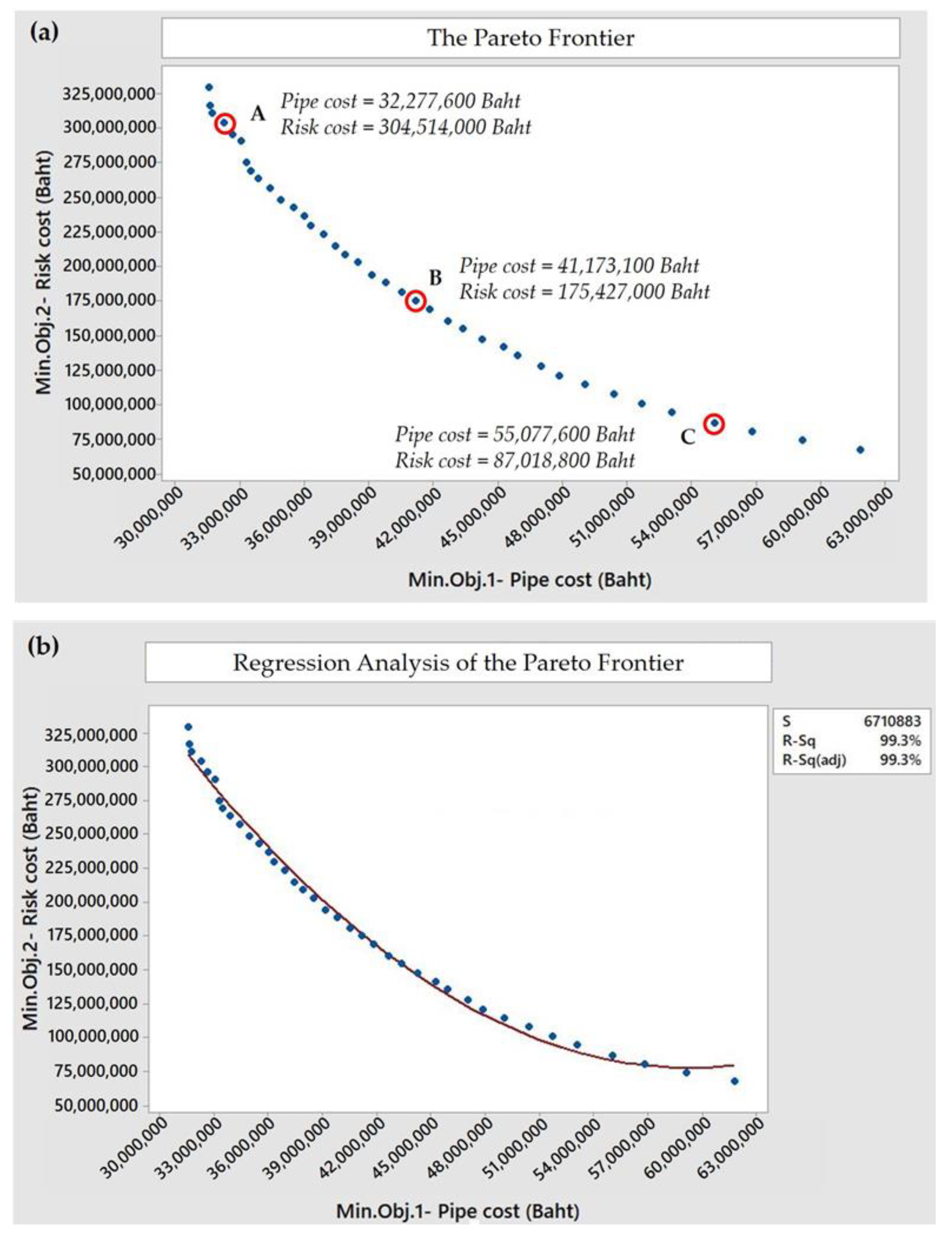
4.2.4. Pareto Frontier Analysis

We next discuss the Pareto frontier obtained from using the Epsilon-constraint method. The Pareto frontier is also known as the non-dominated frontier or efficient frontier in the literature. The Pareto frontier is the set of all non-dominated solutions, which can be graphically shown for any pairs of objective functions. By definition, the Pareto optimal solution in a minimization problem is solution $x^0$ that holds true for $f_k(x) > f_k(x^0)$, which means that $f_j(x) < f_j(x^0)$ for at least one other index j. Likewise, solution $x^0$ is said to be the Pareto optimal solution if $f_k(x) < f_k(x^0)$, meaning that $f_j(x) > f_j(x^0)$ in a maximization problem [39,40,41,42]. Thus, the Pareto optimal solution is a feasible solution that is not dominated by other feasible solutions in which the non-domination property exists such that an improvement in any one objective is possible only at the expense of a poorer solution in at least one other objective. Accordingly, the Pareto frontier can be generated based on a set of Pareto optimal solutions to analyze trade-offs among objective functions in a multi-criteria objective space.

In this study, the Pareto frontier is generated between the pair of cost- and risk-related objective functions, as illustrated in Figure 7a. For instance, the Pareto optimal solution at Point A in the figure indicates that when the desired pipe cost is 32,277,600 Baht, the risk cost required will be 304,514,000 Baht. On the other hand, there is a trade-off such that when the risk cost is improved to 202,922,000 Baht, the pipe cost increases to 38,512,800 Baht, as presented at Point B. Moreover, Point C shows that when the risk cost is improved to 87,018,800 Baht, the required pipe cost will increase to 55,077,600 Baht.

The Pareto frontier can thus be used to visualize the advantages and drawbacks of varying the Epsilon value in the Epsilon-constraint method. Furthermore, we analyzed the polynomial regression model to illustrate the changing trends of the objective functions, which can help predict the objective values, as shown in Figure 7b. The regression model is shown in Equation (81) with an R-squared value of 99.3%, indicating that the variance of the risk cost can be reasonably predicted from the pipe cost. In particular, Figure 8a–c illustrates the plant location in the industrial estate under Pareto Point A, Point B, and Point C, respectively.

$$Z_2 = 1.13E+09 - 35.63(Z_1) + 0.0000001{(Z_1)}^2$$

(81)

5. Managerial Insight

Planning the locations of plants in the industrial estate involves a number of factors. The model developed in this study integrates bi-objective functions between the construction cost based on the piping system and the risk cost as a surrogate criterion for safety. However, other key performance indices can also be used. For example, environmental and social activities can be used as objective functions (e.g., the rate of employment opportunities, public health, and corporate social responsibility) [43,44,45,46]. Considering the model development, four building types are evaluated next, and six comparisons ((4) × (4 − 1)/2) are required to compare all pairs of building types. Thus, converting the non-linear equations to linear forms for the separation requirements requires 24 (6 × 4) associated parameters and variables, which affects the complexity of the developed model. Nonetheless, the problems associated with a larger or smaller number of building types can be adjusted accordingly. In addition, the associated constraint sets pertaining to the separation-distance constraint for the minimum and/or maximum conditions may be relaxed in some cases, which will also affect the computational time of the model.

In the trade-off analysis, the Pareto frontier demonstrates how an improvement in one objective function can worsen the result of the other objective function. The assessed Pareto frontier helps to visualize the effect of increasing emphasis on an objective function of interest. The regression analysis will also allow decision-makers to more easily predict such trade-offs between objective functions. Additionally, given an increasing number of reported emergency situations, accounting for risk management has become an integral part of the planning for an industrial estate. The emergency impact from an explosion and/or fire may cause damage to the surrounding factories inside and outside the industrial estate. Thus, risk management and loss prediction should be analyzed in advance based on the various types of chemical substances in the intended industrial estate.

6. Conclusions and Future Research

This study focused on the design and planning of plant locations in an industrial estate using a case study of an actual industrial estate in Thailand. A bi-objective, mixed-integer linear programming model was proposed and analyzed by considering the economic and safety criteria. Initially, trade-offs between the two objective functions were evaluated by solving a single-objective model. The optimal solution obtained from solving the cost objective showed that the factories should be located close to each other and to the office center. In contrast, the optimal solution from considering only the safety objective function showed that most factories should be dispersed around the boundary of the industrial estate to avoid possible damage in case of an emergency. Thus, trade-offs clearly exist between these two conflicting objective functions. A bi-objective solution was later obtained using the Epsilon-constraint method to further obtain the Pareto optimal solution in this study.

This study provides a practical analysis for the design and planning of an industrial estate. The hazard simulation software called ALOHA was further integrated with the bi-objective optimization model to evaluate the risks and emergencies that could result from the hypothesized leakage and explosion threats of the H₂S chemical substance. By integrating the risk scenario with the developed mathematical model, the software was used to simulate an emergency situation for industrial estate planning. In addition, the developed Pareto frontier was demonstrated so that decision-makers can more easily visualize how improving the safety criterion will affect the cost counterpart when planning an industrial estate. The polynomial regression model was also analyzed to predict the desired objective under a Pareto trade-off.

Future directions of this research include expanding the scope of the study with other case studies including diverse requirements, varied numbers of plants, and different land sizes. Given the present-day complexity of industrial estates, details concerning the technological, functional, business, and technical requirements should also be further explored. For example, piping systems may exhibit material types and characteristics that should be investigated. Other threats obtained from the ALOHA program, including toxic and flammable threats, could also be further used to assess the risk probability and associated damage that may occur. The objectives of interest could also be further expanded to include the three pillars of sustainability, including the social objective. In addition, given a large-scale, multi-objective problem, the exact method implemented in this study may require significant computational time and so the use of metaheuristic algorithms could be further explored to obtain near-optimal solutions in a timely manner. Lastly, the hazard modeling simulation of chemical emergencies implemented in this study could be further used to assess different chemical substances for better risk-management planning.

References

1. Sarkis, J.; Talluri, S. Evaluating and selecting e-commerce software and communication systems for a supply chain. Eur. J. Oper. Res. 2004, 159, 318–329. [Google Scholar] [CrossRef]
2. Puchongkawarin, C.; Ransikarbum, K. An Integrative Decision Support System for Improving Tourism Logistics and Public Transportation in Thailand. Tour. Plan. Dev. 2020, 1–16. [Google Scholar] [CrossRef]
3. Ransikarbum, K.; Pitakaso, R.; Kim, N. A Decision-Support Model for Additive Manufacturing Scheduling Using an Integrative Analytic Hierarchy Process and Multi-Objective Optimization. Appl. Sci. 2020, 10, 5159. [Google Scholar] [CrossRef]
4. Ha, S.; Ransikarbum, K.; Han, H.; Kwon, D.; Kim, H.; Kim, N. A dimensional compensation algorithm for vertical bending deformation of 3D printed parts in selective laser sintering. Rapid Prototyp. J. 2018, 24, 955–963. [Google Scholar] [CrossRef]
5. Busogi, M.; Ransikarbum, K.; Oh, Y.G.; Kim, N. Computational modelling of manufacturing choice complexity in a mixed-model assembly line. Int. J. Prod. Res. 2017, 55, 5976–5990. [Google Scholar] [CrossRef]
6. Singhal, S.; Kapur, A. Industrial estate planning and management in India—an integrated approach towards industrial ecology. J. Environ. Manag. 2002, 66, 19–29. [Google Scholar] [CrossRef] [PubMed]
7. United Nations Conference on Trade and Development (UNCTAD). World Investment Reports 2019: Special Economic Zones; United Nations: Geneva, Switzerland, 2019; Available online: https://unctad.org/ (accessed on 24 February 2020).
8. ASEAN Briefing. Special Economic Zones in ASEAN: Opportunities for US Investors. Available online: https://www.aseanbriefing.com/ (accessed on 31 January 2021).
9. Industrial Estate Authority of Thailand (IEAT). Annual Report 2018. Available online: https://www.ieat.go.th/ (accessed on 29 December 2019). (In Thai)
10. Galbraith, C.; De Noble, A.F. Location decisions by high technology firms: A comparison of firm size, industry type and institutional form. Entrep. Theory Pract. 1989, 13, 31–48. [Google Scholar] [CrossRef]
11. Buoro, D.; Casisi, M.; De Nardi, A.; Pinamonti, P.; Reini, M. Multicriteria optimization of a distributed energy supply system for an industrial area. Energy 2013, 58, 128–137. [Google Scholar] [CrossRef]
12. Alves, D.T.S.; de Medeiros, J.L.; Ofelia de Queiroz, F.A. Optimal determination of chemical plant layout via minimization of risk to general public using Monte Carlo and Simulated Annealing techniques. J. Loss Prev. Process Ind. 2016, 41, 202–214. [Google Scholar] [CrossRef]
13. Hosseinnia, B.; Khakzad, N.; Reniers, G. Multi-plant emergency response for tackling major accidents in chemical industrial areas. Saf. Sci. 2018, 102, 275–289. [Google Scholar] [CrossRef]
14. Ransikarbum, K.; Kim, N.; Ha, S.; Wysk, R.A.; Rothrock, L. A highway-driving system design viewpoint using an agent-based modeling of an affordance-based finite state automata. IEEE Access 2017, 6, 2193–2205. [Google Scholar] [CrossRef]
15. Chanthakhot, W.; Ransikabum, K. Numerical Simulation for Fire Emergency Planning in a Home Appliances Factory. In Proceedings of the 2019 Research, Invention, and Innovation Congress, Bangkok, Thailand, 11–13 December 2019; pp. 1–5. [Google Scholar]
16. Kim, J.; Ransikarbum, K.; Kim, N.; Paik, E. Agent-based simulation modeling of low fertility trap hypothesis. In Proceedings of the 2016 ACM SIGSIM Conference on Principles of Advanced Discrete Simulation, Banff, AB, Canada, 15–18 May 2016; pp. 83–86. [Google Scholar]
17. Caputo, A.C.; Pelagagge, P.M.; Palumbo, M.; Salini, P. Safety-based process plant layout using genetic algorithm. J. Loss Prev. Process Ind. 2015, 34, 139–150. [Google Scholar] [CrossRef]
18. Chae, J.; Regan, A.C. Layout design problems with heterogeneous area constraints. Comput. Ind. Eng. 2016, 102, 198–207. [Google Scholar] [CrossRef]
19. Wu, Y.; Wang, Y.; Feng, X. A heuristic approach for petrochemical plant layout considering steam pipeline length. Chin. J. Chem. Eng. 2016, 24, 1032–1037. [Google Scholar] [CrossRef]
20. Xu, Y.; Wang, Z.; Zhu, Q. An improved hybrid genetic algorithm for chemical plant layout optimization with novel non-overlapping and toxic gas dispersion constraints. Chin. J. Chem. Eng. 2013, 21, 412–419. [Google Scholar] [CrossRef]
21. Medina-Herrera, N.; Jiménez-Gutiérrez, A.; Grossmann, I.E. A mathematical programming model for optimal layout considering quantitative risk analysis. Comput. Chem. Eng. 2014, 68, 165–181. [Google Scholar] [CrossRef] [Green Version]
22. de Lira-Flores, J.A.; Gutierrez-Antonio, C.; Vázquez-Román, R. A MILP approach for optimal storage vessels layout based on the quantitative risk analysis methodology. Process Saf. Environ. Prot. 2018, 120, 1–13. [Google Scholar] [CrossRef]
23. Rahman, S.M.T.; Salim, M.T.; Syeda, S.R. Facility layout optimization of an ammonia plant based on risk and economic analysis. Procedia Eng. 2014, 90, 760–765. [Google Scholar] [CrossRef] [Green Version]
24. Patsiatzis, D.I.; Knight, G.; Papageorgiou, L.G. An MILP approach to safe process plant layout. Chem. Eng. Res. Des. 2004, 82, 579–586. [Google Scholar] [CrossRef]
25. Jung, S.; Ng, D.; Laird, C.D.; Mannan, M.S. A new approach for facility siting using mapping risks on a plant grid area and optimization. J. Loss Prev. Process Ind. 2010, 23, 824–830. [Google Scholar] [CrossRef]
26. Han, K.; Cho, S.; Yoon, E.S. Optimal layout of a chemical process plant to minimize the risk to humans. Procedia Comput. Sci. 2013, 22, 1146–1155. [Google Scholar] [CrossRef] [Green Version]
27. Ahumada, C.B.; Quddus, N.; Mannan, M.S. A method for facility layout optimization including stochastic risk assessment. Process Saf. Environ. Prot. 2018, 117, 616–628. [Google Scholar] [CrossRef]
28. Yoon, K.; Hwang, C.L. Manufacturing plant location analysis by multiple attribute decision making: Part I—Single-plant strategy. Int. J. Prod. Res. 1985, 23, 345–359. [Google Scholar] [CrossRef]
29. Wang, R.; Wu, Y.; Wang, Y.; Feng, X. An industrial area layout design methodology considering piping and safety using genetic algorithm. J. Clean. Prod. 2017, 167, 23–31. [Google Scholar] [CrossRef]
30. Wattanasaeng, N.; Ransikarbum, K. Cost Optimization Model for Plant Assignment in Industrial Estate Planning. In Proceedings of the 2019 Research, Invention, and Innovation Congress, Bangkok, Thailand, 11–13 December 2019; pp. 1–6. [Google Scholar]
31. Wattanaseang, N.; Ransikarbum, K. Sites Selection of industrial estates for Thailand Border’s Special Economic Zones using Data Envelopment Analysis. UBU Eng. J. 2020, 13, 14–26. (In Thai) [Google Scholar]
32. Bai, Q.; Labi, S.; Sinha, K.C. Trade-off analysis for multi-objective optimization in transportation asset management by generating Pareto frontiers using extreme points nondominated sorting genetic algorithm II. J. Transp. Eng. 2012, 138, 798–808. [Google Scholar] [CrossRef]
33. Mavrotas, G. Effective implementation of the ε-constraint method in multi-objective mathematical programming problems. Appl. Math. Comput. 2009, 213, 455–465. [Google Scholar] [CrossRef]
34. Toro, E.M.; Franco, J.F.; Echeverri, M.G.; Guimarães, F.G. A multi-objective model for the green capacitated location-routing problem considering environmental impact. Comput. Ind. Eng. 2017, 110, 114–125. [Google Scholar] [CrossRef] [Green Version]
35. Abounacer, R.; Rekik, M.; Renaud, J. An exact solution approach for multi-objective location–transportation problem for disaster response. Comput. Oper. Res. 2014, 41, 83–93. [Google Scholar] [CrossRef] [Green Version]
36. Yu, H.; Solvang, W.D. An improved multi-objective programming with augmented ε-constraint method for hazardous waste location-routing problems. Int. J. Environ. Res. Public Health 2016, 13, 548. [Google Scholar] [CrossRef] [Green Version]
37. Ministry of Commerce (MOC). Total Construction Material Price. Available online: http://www.indexpr.moc.go.th/ (accessed on 3 March 2019). (In Thai)
38. Thai Appraisal and Estate Agents Foundation (TAEAF). The 2018 Costs of Constructions. Available online: https://www.thaiappraisal.org/ (accessed on 3 March 2019). (In Thai).
39. Ransikarbum, K.; Mason, S.J. Multiple-objective analysis of integrated relief supply and network restoration in humanitarian logistics operations. Int. J. Prod. Res. 2016, 54, 49–68. [Google Scholar] [CrossRef]
40. Ransikarbum, K.; Mason, S.J. Goal programming-based post-disaster decision making for integrated relief distribution and early-stage network restoration. Int. J. Prod. Econ. 2016, 182, 324–341. [Google Scholar] [CrossRef]
41. Ransikarbum, K.; Ha, S.; Ma, J.; Kim, N. Multi-objective optimization analysis for part-to-Printer assignment in a network of 3D fused deposition modeling. J. Manuf. Syst. 2017, 43, 35–46. [Google Scholar] [CrossRef]
42. Ransikarbum, K. Decision Analysis for Engineering; Chulalongkorn University Printing House: Bangkok, Thailand, 2021; in press. [Google Scholar]
43. Chaiyaphan, C.; Ransikarbum, K. Criteria analysis of food safety using the Analytic Hierarchy Process (AHP)-a case study of Thailand’s fresh markets. In Proceedings of the 2019 Research, Invention, and Innovation Congress, Bangkok, Thailand, 11–13 December 2019; pp. 1–7. [Google Scholar]
44. Ransikabum, K.; Yingviwatanapong, C.; Leksomboon, R.; Wajanavisit, T.; Bijaphala, N. Additive Manufacturing-based Healthcare 3D Model for Education: Literature Review and A Feasibility Study. In Proceedings of the 2019 Research, Invention, and Innovation Congress, Bangkok, Thailand, 11–13 December 2019; pp. 1–6. [Google Scholar]
45. Xu, J.; Song, X. Multi-objective dynamic layout problem for temporary construction facilities with unequal-area departments under fuzzy random environment. Knowl. Based Syst. 2015, 81, 30–45. [Google Scholar] [CrossRef]
46. Tajbakhsh, A.; Shamsi, A. A facility location problem for sustainability-conscious power generation decision makers. J. Environ. Manag. 2019, 230, 319–334. [Google Scholar] [CrossRef] [PubMed]
Figure 1. Schematic diagram for the proposed methodology.
Computation 09 00046 g001
Figure 2. Flow diagram of the Epsilon-constraint method.
Computation 09 00046 g002
Figure 3. Radius of the chemical analysis from the Areal Locations of Hazardous Atmospheres (ALOHA) program based on the (a) toxic threat zone, (b) flammable threat zone, and (c) overpressure threat zone.
Computation 09 00046 g003
Figure 4. The case study: (a) industrial estate layout and (b) simulated ALOHA’s explosion with computed risk probability.
Computation 09 00046 g004
Figure 5. Plant location in the industrial estate under the cost objective.
Computation 09 00046 g005
Figure 6. Plant location in the industrial estate under the risk objective.
Computation 09 00046 g006
Figure 7. (a) The Pareto frontier. (b) Regression model of the Pareto frontier.
Computation 09 00046 g007
Figure 8. Plant location under (a) Pareto Point A, (b) Pareto Point B, and (c) Pareto Point C.
Computation 09 00046 g008