Article

Stabilization of the Computation of Stability Constants and Species Distributions from Titration Curves

Materials and Surface Engineering Group, Institute of Materials Science and Engineering, Chemnitz University of Technology, D-09107 Chemnitz, Germany
*
Author to whom correspondence should be addressed.
Computation 2021, 9(5), 55; https://doi.org/10.3390/computation9050055
Submission received: 1 April 2021 / Revised: 20 April 2021 / Accepted: 26 April 2021 / Published: 27 April 2021
(This article belongs to the Section Computational Chemistry)

Abstract

:
Thermodynamic equilibria and concentrations in thermodynamic equilibria are of major importance in chemistry, chemical engineering, physical chemistry, medicine etc. due to a vast spectrum of applications. E.g., concentrations in thermodynamic equilibria play a central role for the estimation of drug delivery, the estimation of produced mass of products of chemical reactions, the estimation of deposited metal during electro plating and many more. Species concentrations in thermodynamic equilibrium are determined by the system of reactions and to the reactions’ associated stability constants. In many applications the stability constants and the system of reactions need to be determined. The usual way to determine the stability constants is to evaluate titration curves. In this context, many numerical methods exist. One major task in this context is that the corresponding inverse problems tend to be unstable, i.e., the output is strongly affected by measurement errors, and can output negative stability constants or negative species concentrations. In this work an alternative model for the species distributions in thermodynamic equilibrium, based on the models used for HySS or Hyperquad, and titration curves is presented, which includes the positivity of species concentrations and stability constants intrinsically. Additionally, in this paper a stabilized numerical methodology is presented to treat the corresponding model guaranteeing the convergence of the algorithm. The numerical scheme is validated with clinical numerical examples and the model is validated with a Citric acid–Nickel electrolyte. This paper finds a stable, convergent and efficient methodology to compute stability constants from potentiometric titration curves.

1. Introduction

The measurement, simulation, and evaluation of species distributions in thermodynamic equilibria and potentiometric titration curves are of special interest in research as they indicate the behavior of reactions taking place at different pH values, cf. [1,2]. The stability constants of the considered reactions and the concentration distribution of the given species over the pH values are of particular interest. For example, in the electrolyte design, a major indicator of the deposition speed is the free metal concentration in thermodynamic equilibrium in the electrolyte at a certain pH value, see [3]. Additionally, the free metal concentrations in thermodynamic equilibrium are commonly used as boundary data for simulations of metal deposition while electro plating, see [4,5,6,7]. For this the stability constants are needed, which are commonly computed from titration curves, see [8,9,10,11,12].
A common way to compute stability constants, as applied in the work of Xu et al. [8] and the work of Zanonato et al. [9], is through the application of DFT (density functional theory) methods as described in the work of Becke [10], which is based on the approximation of the density functional describing the exchange-energy density of atomic and molecular systems. Although this strategy is time-efficient, in this paper a numerical strategy will be constructed to unify the calculation of titration curves with the inverse calculation of the stability constants by reconstructing the titration curves themselves. In addition to the unification of the approaches for the computation of titration curves and stability constants, the approach chosen in this paper has three major additional advantages. The first advantage is that the presented algorithm and model immediately produces concentration distributions over the pH values without additional computation steps. The second advantage is the closeness of the theoretical model to the measured chemical process. The third advantage is that the approach discussed in this paper yields a robust numerical strategy for the inverse problem, which is known to be unstable, see [13,14].
The model for the computation of the titration curve used in this paper is based on the model formulation in the articles of Alderighi et al. and Gans et al. [11,12] and in the work of Langtangen [15], but it will be equivalently reformulated to stabilize the model formulation. This is needed since inverse problems such as the one used to calculate the stability constants tend to be unstable from a mathematical perspective, see Hinze et al. [13] and Richter [14]. In the work of Alderighi [11], the numerical scheme is described by a simple application of the Newtonian algorithm, which is known to be unstable, see the book of Mäkelä et al. and Lange [16,17], in this paper, an algorithm will be discussed which is more stable based on homotopy methods, see [18,19].
Similar to as in the book of Martell [20], the simulated titration curves are used to calculate the stability constants from measured titration curves. However, in contrast to the numerical scheme described in [11,12,20], the numerical scheme described in this article is based on the treatment of the stabilized formulation of the titration curve.
Due to the stabilized formulation of the titration curve, an increase in robustness and reliability of the results of the stability constants is gained.
An important application for the evaluation of titration curves, inverse calculated stability constants, and the species distributions under the pH value is given by the work of Cesiulis [3], which gives a methodology to identify the pH-value with the current density j during electrodeposition with the stability constants being used to compute the free metal concentrations. This requires chemical and numerical considerations. To accomplish this, a closer look at the electrolyte is needed, in particular in terms of the chemical equilibrium and the law of mass action, see [21]. The law of mass action, also referred to as the mass-conservation law, forms the basis for both equilibrium and kinetic investigations. This is based on activities. However, the experiments and calculations presented in this paper are based on concentrations. The difference between concentration and activity is determined by the activity coefficient, which is difficult to determine experimentally [22]. By default, this difficulty is circumvented by working with constant ionic strength, since the activity coefficients are largely dependent on it, and equilibrium constants can thus be more easily recorded. However, the ionic strength does not stay constant during a reaction. Additionally, the addition of “inert” salts could influence the reaction. The desired equilibrium constants could be determined with infinite dilution; from a practical perspective, however, infinite dilution is unfeasible/impossible. The attractive forces between the ions acting in more concentrated solutions result in dissolved particles no longer moving completely independently of each other, as would be the case for ideal solutions [23]. In an ideally diluted solution of an electrolyte, the probability of encountering another cation or anion in the vicinity of a cation should be equally high because the ions do not influence each other. As the concentration increases, more orderly ratios gradually begin to form, i.e., an anion is more likely to be found in the vicinity of the cation and vice versa. In real solutions, the dissolved particles are no longer completely free to move. Therefore, lower concentrations are simulated. However, only the mean activity coefficient can be determined. This is not only dependent on the concentration of the own ions but also on the concentration of all ions present in the solution. The determination of the equilibrium constant using the law of mass action, as shown in this work, takes all the species present into account. Since these are dependent on the established chemical equilibrium, it is assumed that once a stable equilibrium system has been reached at any point on the titration curve, the determination of the activity can be dispensed with in favor of observing the concentrations in the case of equilibrium. Similar to the contribution of Karimvand et al. [24], this article proposes an approach where thermodynamic equilibrium constants are determined directly from the analysis of potentiometric pH titrations. However, this approach avoids the use of activity coefficients by determining the individual points of the potentiometric titration at any time in thermodynamic equilibrium. For this purpose, the adjustment of the equilibrium is monitored “intelligently” by letting the system reach its equilibrium before the base is added in the next titration step. From this, a simulation of the titration curves is carried out by means of a robust numerical method, and the thermodynamic stability constants are calculated from the law of mass action.

2. Experimental Methodology-Intelligent Potentiometric Titration

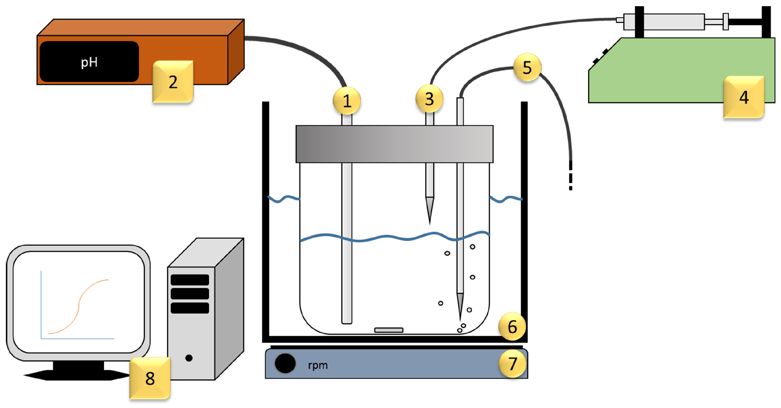
Two real-life problems are discussed in this work to validate the framework of the models described. For this purpose, potentiometric pH titrations were performed. The ”intelligent“, i.e., automatically controlled, potentiometric pH titration was carried out at a constant temperature of 25 °C and with the intake of argon ( Ar 99.9999 % , Alphagaz™Air Liquide), shown in Figure 1. These were performed first with an electrolyte containing only citric acid and then with a citric acid-nickel electrolyte. Each titration was performed in 0.1 L ultrapure water ( < 0.1 μ S cm , Barnstead™Smart2Pure™, Thermo Fisher Scientific Inc. Waltham, MA, USA). For the first titration of pure citric acid, a quantity of 0.001 mol citric acid ( C 6 H 8 O 7 · H 2 O , >99.5%, Th. Geyer GmbH & Co. KG.) was added and the solution was adjusted to pH = 2 using sodium hydroxide (NaOH, 1 N , 99.99%, ABCR GmbH). Afterwards, V = 0.25 m L NaOH was added in stages (doses) in areas with fast equilibrium setting and V = 0.1 mL NaOH in areas with slow equilibrium setting. For the titration of citric acid-nickel, a solution with 0.001 mol citric acid and 0.00083 mol nickel from nickel chloride ( NiCl 2 · 6 H 2 O , >99.8%, ABCR GmbH) was provided and carried out in the same way as with the previous titration. All measurements were repeated three times for statistical confirmation and significance.
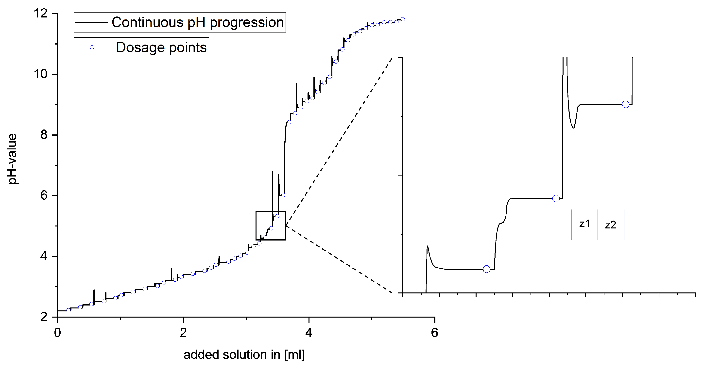
A special feature of this titration procedure is the ability to adjust the timing of the next dose of the respective base based on real-time observation of the equilibrium setting, as shown in Figure 2. After each addition, the equilibrium setting was monitored by means of automated measurement of the potential curve. Only when the potential curve showed no further increase was the next dosage carried out. This is necessary to guarantee the final adjustment of the equilibrium state, depending on thermodynamic and kinetic reaction influences. To exclude the influence of the background noise of the potential measurement, two ranges with time comparison values z 1 and z 2 are defined in the potential curve after the dosing z 1 + z 2 , and the increases of these two ranges are compared with each other. If the curve shows the same increase in both time periods, the equilibrium setting continues to run evenly, and two new time units are formed during the potential. Only when the rise of the second time unit approaches zero is the equilibrium setting complete and the next dose given. Due to the variability regarding the timing of the base addition, the optimum amount of base can always be given.
Based on this experimental system, the following numerical considerations could be made.

3. Modeling

This section is devoted to the derivation of a stable and robust model formulation for the simulation of thermodynamic equilibria, titration curves, and the inverse determination of the associated Michaelis constants, referred to as stability constants in this paper. Although the model type discussed in this article will be confined to aqueous media, other generalized models and concepts are conceivable but would require minor modifications from the discussion below.

3.1. Concentrations in Thermodynamic Equilibria

First, assuming that there are # L N ligands L 1 , …, L # L and # M metals M 1 , …, M # M , protons H + and hydroxide ions OH are given in solution as educts. Furthermore, assume that the following R N reactions take place in the electrolyte:
j = 1 # L l j , κ L j + k = 1 # M m k , κ M k + h κ H + o κ OH j = 1 # L L j l j , κ k = 1 # M M k m k , κ OH o κ H h κ = : K κ , 1 κ R ,
where for all 1 κ R the species K κ denote the product of the κ -th reaction. Furthermore, let l j , κ N be the stoichiometric index of the j-th ligand in the κ -th reaction. Analogously, let m k , κ N be the stoichiometric index of the k-th metal in the κ -th reaction. In addition, the stoichiometric index of H + in the κ -th reaction is denoted by h κ N and o κ N denotes the stoichiometric index of OH in the κ -th reaction.
For the simplicity of the notation of the following discussion, define the educts E 1 : = L 1 , …, E # L : = L # L , E # L + 1 : = M 1 , …, E # L + # M : = M # M , E # L + # M + 1 : = H + , and E # L + # M + 2 : = OH . The stoichiometric indices e j , κ denote the respective stoichiometric indices of the single species. In this notation, the reaction (1) reduces to the simpler formula given below:
j = 1 N e j , κ E j , κ j = 1 N E j e j , κ = K κ , 1 κ R
As a foundation of the model discussed in this paper, the following mass-conservation laws, see [15], for given total masses m E j , including free species concentrations and species in complexes, of the educt E j is given by:
c E j + κ = 1 R e j , κ c K κ = m E j , 1 j N .
In the notation above, the values c E j denote the free masses of the educt E j , and c K κ denotes the masses of the complexes K κ .
One obtains a system of N non-linear equations in N + R variables. The system above can be solvable but not uniquely. To obtain a system of uniquely solvable equations, one needs to add R additional equations. In this setting, one directly uses the definition of the stability constant, which is equivalent to the following system of equations, see [15]:
c K κ = β κ j = 1 N c E j e j , κ , 1 κ R .
In fact, Equations (3a) and (3b) directly build up a model for thermodynamic equilibria due to the reactions given in (2). Please note that one can also equivalently formulate the non-linear Equations (3a) and (3b) in terms of concentrations rather than in terms of masses.
Due to the fact that the stability constants β κ can reach values up to 10 50 , the model formulation tends to be unstable from a numerical perspective. Hence, a further reformulation of the model must be made to stabilize the mathematical formulation.
For the mathematical reformulation, note that under the assumptions
0 < β κ , 1 κ R ,
0 < c E j , c K κ , 1 j N , 1 κ R ,
there exist b κ R , x j R and y κ R such that the following identities hold true:
c E j = exp ( x j ) , 1 j N and
β κ = exp ( b κ ) , c K κ = exp ( y κ ) , 1 κ R
Using the identities above, especially (4c) and (4d), the model described by Equations (3a) and (3b) transforms to the following model equations:
0 = exp ( x j ) + κ = 1 R e j , κ exp ( y κ ) S E j , 1 j N and
0 = b κ y κ + j = 1 N e j , κ x j , 1 κ R
The resulting formulation of a single thermodynamic equilibrium yields a more stable formulation of the mass-conservation law.
For the solution of (5a) and (5b), the formulation for the determination of roots of the function f b : R # L + # R + 2 R # L + # R + 2 , reflecting (5a) and (5b) regarding the variables (4c) and (4d).
Remark 1.
The following remarks must be made:
1. 
The models corresponding to Equations (5a) and (5b) and (3a) and (3b) both correspond to a search of roots of non-linear functions. The corresponding mathematical problems are constructed to be equivalent, meaning that each solution of (5a) and (5b) can uniquely be identified to a solution to (3a) and (3b) and vice versa, see (4c) and (4d).
2. 
For the well-posedness of the model given through Equations (5a) and (5b) the following assumptions are sufficient.
(A1) 
The variables ( x , y ) R N + R are independent, i.e., the single variables are referring to unique concentration.
(A2) 
The single equations are (linear) independent from each other, i.e., describe the behavior of a uniquely determined setting, i.e., there is no doubling in the reactions (2).
(A3) 
The total masses m E j are positive for each 1 j N .
3. 
In general, the numerical treatment of the model associated with Equations (5a) and (5b) becomes necessary as it follows from the mathematical theory that there is no general formula to calculate roots of polynomials with coefficients in R for a polynomial degree larger or equal to 5, see [25].
4. 
Please note that the model associated with Equations (5a) and (5b) where derived from (3a) and (3b), under the assumption of positive concentrations, by changing the variables into logarithms. The advantage, besides the numerical stability of the new formulation it grants intrinsic positive species concentrations. This is for (3a) and (3b) in general not given, since there usually exist negative roots to (3a) and (3b), see [25]. Please note that the species distributions and the inclusion of complexes guarantee the positivity of the complex formation constants. This avoids the necessity to use more complicated and more cost-intensive numerical methods, such as described in this paper, such as augmented Lagrangian algorithms, see [26,27].
5. 
The model formulation used in this paper (5a) and (5b) differs not only in the introduction of logarithms into the problem formulation, but it also differs from the model formulations used in the works of Alderighi et al., Gans et al. and Martell [11,12,20], by considering the complexes as well. This is commonly omitted by inserting (3b) into (3a).

3.2. A Model of Titration Curves with Vertices in Thermodynamic Equilibrium

The aim of this section is the modeling of the potentiometric titration curves as they are obtained from the experimental set-up described in Section 2. First, assume that ligands L 1 , …, L # L , metals M 1 , …, M # M , hydroxide ions OH , and protons H + are given in the original electrolyte. Additionally, suppose that R N reactions in the form of (1) take place.
As described in the experimental set-up described in Section 2, a starting volume 0 < V 0 of electrolyte is assumed to be given, with given total masses m L j , 0 , in mol of the ligand L j , for 1 j # L , total masses m M k , 0 of the metal M k , for 1 k # M , and the total mass of hydroxide ions m O H 0 in mol of OH as well as the total masses of the protons H + m H 0 in the electrolyte.
Furthermore, suppose that Z N additions of a solution, with molar concentration c a d d , OH in mol l of OH concentration, and suppose that no additional species other than H + , OH and H 2 O are interacting with the assumed system of reactions (1). Additionally, suppose that the solution is added in the following volume steps: 0 = v 0 v 1 v Z R 0 .
Due to the experimental set-up, it can be assumed that in each chosen measurement, a state close to the thermodynamic equilibrium is reached. Due to the assumptions above, one can describe the concentrations in each measured state through the model given by Equations (5a) and (5b). To describe the respective models, it is left to describe the total masses m M k , z , m L j , z , m H z + , and m OH z in each added volume v z for 1 z Z of the solution above.
Due to the assumptions about the added solution described above, one finds that the masses m M k , z and m L j , z do not change over the titration, i.e., for all 1 z Z , for all 1 k # M , and all 1 j # L , i.e., one obtains
m M k , z = m M k , 0 , 1 k # M , 1 z Z ,
m L j , z = m L j , 0 , 1 k # L , 1 z Z .
Furthermore, under the usage of l z = log 10 ( z a d d , OH ) , and for
d P : = log 10 c H + c OH = log 10 β H 2 O c H 2 O ,
where β H 2 O is the complex formation constant of water, the exact value for 25 °C is given in Equation (19), where d P is the deprotonation constant and
c OH = z a d d , OH mol l = 10 l z mol l and c H + , a d d = 10 ( d P l z ) mol l ,
where c OH , a d d denotes the concentration of the hydroxide ions of the added solution and c H + , a d d the concentration of the protons. Then, the total masses m O H z and m H z of the electrolyte after the z-th addition of the given solution are described by
m O H z = m O H 0 + v z c H 2 O c H + , a d d = m O H 0 + v z c H 2 O 10 ( d P l z ) , 1 z Z and
m H z = m H 0 + v z c H 2 O c OH , a d d = m O H 0 + v z c H 2 O 10 l z , 1 z Z .
Combining the model with the RHS (6a)–(6f), one obtains for each measurement point 1 z Z a model for the thermodynamic equilibrium. This yields a complete model for the titration curve, under the assumption that the stability constants 0 < β κ are given for each reaction 1 κ R .
This set-up yields a set of Z systems of # L + # M + 2 + R non-linear equations which directly describe the molar masses of the species as variables for the RHS as input data, which must be solved to obtain the molar masses at each step, i.e., one has to solve a system of non-linear equations in the following form:
F b ( y ) = F 0 , b ( y 0 ) F z , b ( y z ) F Z , b ( y Z ) = 0 ,
where F z : R # M + # L + 2 + R R # M + # L + 2 + R is, for all 1 z Z , the function given by the non-linear model (5a) and (5b), with variables as denoted by (4c) and (4d) and RHS given by (6a)–(6f) for fixed stability constants
[ exp ( b 1 ) , , exp ( b R ) ] T = [ β 1 , , β R ] T : = β R > 0 R .
The Equation (7) can be used to fit the titration curve regarding the variables b 1 , …, b R to the measured titration curve as given by the measurement as described in Section 2.

3.3. Calculation of the Total Masses m H 0 and m O H 0

In many relevant cases, the total masses of m O H 0 and m H 0 are unknown. In this section, a way to calculate m O H 0 and m H 0 will be detailed. For this, it should be noted that in the measurement of the titration curve, the pH value of the initial volume of the electrolyte is given. Hence, the concentrations c H + and c OH are known. These values will be used to determine m O H 0 and m H 0 .
The way to calculate the values of m O H 0 and m H 0 is to take the first equation, corresponding to the 0-th addition during titration, as given in Section 3.2 and with the interpretation of m O H 0 and m H 0 as variables and then interpret the given values of log c H + and log c OH as input data to finally obtain a system of # L + # M + 2 + R equations in # L + # M + 2 + R variables which must be solved. As part of the corresponding solution, one obtains values for m H 0 and m O H 0 .
When formalizing the strategy above, one obtains a non-linear system of equations in the following form:
F ¯ 0 y ¯ 0 = 0 ,
In the equation above, the function F ¯ 0 : R # L + # M + 2 R # L + # M + 2 is the function associated with the model given by (5a) and (5b) where the variables y ¯ 0 ( 1 ) , …, y ¯ 0 ( # L + # M ) are corresponding to
y ¯ 0 ( # M + j ) = log c L j , 1 j # L . and
y ¯ 0 ( k ) = log c M k , 1 k # M
Additionally, the variables y ¯ 0 ( # L + # M + 1 ) and y ¯ 0 ( # L + # M + 2 ) are given through
y ¯ 0 ( # L + # M + 1 ) = m H 0 and
y ¯ 0 ( # L + # M + 2 ) = m O H 0 .
This yields a system of functions from which m H 0 and m O H 0 can be determined.

3.4. Formulating an Inverse Problem

As discussed in the introduction, this paper aims at a method to calculate the stability constants β R R associated with the reactions given in (2). In this section, an inverse problem, as in the books of Hinze et al., Richter [13,14] or in the book of Mäkelä [16], will be derived.
Assume that M N measurements of the pH values p H ¯ 1 , , p H ¯ M are given. Furthermore, for an arbitrary fixed b R > 0 R , let the vector y b * R Z ( # M + # L + 2 ) be the solution to (7). Then, the to b associated pH values
p H 1 ( b ) , , p H M ( b ) T = log 10 ( exp ( y b , ( j 1 ) R + # M + # L + 1 ) ) j = 1 Z
can be interpreted as the image of a vector-valued function
b g ( b ) = [ g 1 ( b ) , , g Z ( b ) ] T = p H 1 ( b ) , , p H Z ( b ) T .
Then, one seeks a b R R for which the following residual is minimal:
res ( b ) : = z = 1 Z | p H z ¯ g j ( b ) |
In many cases, the values of b can be restrained. For most applications, stability constants β can be restricted to 10 50 = lb β ub = 10 50 .
When translating the setting above into a restrained minimization problem, one seeks the solution b to the following restrained minimization problem:
b = error b ^ R R z = 1 M | p H z ¯ g z ( b ^ ) | = 0 s . t . : log ( lb ) b ^ κ log ( ub ) .
Then, the stability constants β are given as
[ β 1 , , β R ] = [ exp ( b 1 ) , , exp ( b R ) ] .
Hence, a minimization problem was derived whose solution can be reformulated into the searched stability constants.

3.5. An Inherent Method to Validate the Assumed Reaction System

In practice, an important question is how to validate an assumed system of reactions. In the following, a way to validate the system of reactions (1) will be discussed:
Suppose that the reaction
H + OH H 2 O
is considered in the calculations of the thermodynamic equilibrium and the minimization (14). Then, at room-temperature, the identity
c H + c OH = 10 13.79
holds true. For the discussion, it should be noted that the molar weight of water is given by the molar weights of two protons, which has a molar weight of 1.008 g mol and an oxygen atom, which has a molar weight of 15.999 g mol . With the data above and taking into account that one liter of water has a weight of 1000 g, one obtains the following concentration of water in water:
c H 2 O = 1000 g 18.015 g mol l = 55.507 mol l
With the equation above and the usage of the deprotonation constant of water log 10 c H c OH = 13.79 , one obtains the following verification identity:
log 10 β H 2 O = c H 2 O c H c OH log 10 55.507 10 13.79 = 15.5343 .
Although the calculation above was done for the concentration of pure water of c H 2 O , the value of log 10 β H 2 O can be used to validate the reaction systems and additional stability constants.

4. Numerical Methodology

In this section, the numerical strategy to simulate the thermodynamic equilibria, titration curves, and the inverse problems will be discussed. Based on the simulation of thermodynamic equilibria, see Section 4.1, a method for the prediction of titration curves will be derived, see Section 4.2. Additionally, in Section 4.3, the calculation of the RHS parts associated with m O H 0 and m H 0 will be discussed as well as the numerical methodology of the evaluation of the inverse problem in Section 4.4.

4.1. Simulation of Thermodynamic Equilibria

This section is devoted to the description of the numerical treatment and approximation of the non-linear systems of equations associated with the model (5a) and (5b), as given by the determination of roots of the function f b : R # L + # R + 2 R # L + # R + 2 as it is defined in Section 3.1.
An initial idea for the treatment of the zero search could be, as done in the work of Alderighi et al. or Martell [11,20], a direct application of a Newtonian scheme, see [28]. Since the convergence of classical Newtonian schemes is only granted when the starting value x 0 of the algorithm is member of a sufficient close neighborhood of the searched zero x * R # M + # L + R , see [17,29], | x 0 x * | 2 < ε for ε < ε 0 must be fulfilled. The major issue is that x * and 0 < ε 0 are generally unknown. Since a sufficiently good starting value is unknown in the first instance, the Newtonian scheme cannot be applied directly in most cases. A solution to this problem is the usage of stabilized Newtonian schemes as described in [30].
The stabilized Newtonian schemes converge for each given x 0 , but the efficiency of the stabilized Newton methods still depends on the initial value, although it is relatively complicated. In practice, the stabilized Newton methods need rather long computation times.
Therefore, it is not a stabilized Newton scheme described in this article but instead an easier method based on a homotopy method, see [18,19]. The basic idea of the homotopy method is to calculate an appropriate initial value for the Newtonian scheme. A central point is the use of continuous deformation from a simpler function g : R # L + # M + 2 + R R # L + # M + 2 + R , for which a zero is known, to f b .
In this paper, the function g is the identity function. Furthermore, a deformation in the form
H : R # M + # L + 2 + R × [ 0 , 1 ] R # M + # L + 2 + R ,
( x , t ) t f t · b ( x ) + ( 1 t ) x .
is used.
Now, let a decomposition T : = { t 0 , , t N } , with N N and 0 = t 0 < < t N = 1 be given. Then in each step the system of nonlinear equations is solved:
Find x * x * R # M + # L + 2 + R
H ( x * , t k ) = 0 .
Then, one applies the following Algorithm 1:
Algorithm 1: Homotopy Loop
Input: Initial value x 0 R # M + # L + 2 + R , tolerance 0 < ε , a decomposition T , length L : = | T | of the decomposition and set k = 0 .
Output: Approximate solution to H ( x , 1 ) = 0 .
Perform the following steps:
S 1
Approximate a solution of x, with tolerance ε , and initial value x 0 to the following problem with the Newtonian scheme given in Appendix A.
Find x * R # M + # L + 2 + R such that it fulfills (21).
As output of the Newtonian scheme, one obtains an approximation x ε * of x * and an error e r r .
S 2
If err ε and k < L set k : = k + 1 , x 0 : = x * and go to S 1. If k = L and err ε then go to S 4. If err > ε then go to S 3.
S 3
Use a finer decomposition T ^ of [ 0 , 1 ] than beforehand, meaning with greater length L < | T ^ | , and set L : = | T | , T T ^ and set L : = T ^ .
Remark 2.
1. Please note that the identities H ( x , 0 ) = g ( x ) = x and H ( x , 1 ) = f b ( x ) directly imply that the output of Algorithm 1 is a sufficiently good approximation x ε * of the initially searched zero of f b .
2. 
Additionally, note that the stability issues of the Newtonian scheme are solved by the homotopy Algorithm 1 if the decomposition T is sufficiently fine, and one can grant convergence independently from the initial value.
3. 
In contrast to the numerical schemes described in Alderighi et al., Gans et al., or Martell [11,12,20], where a simple Newtonian scheme is used, in this paper the homotopy Algorithm 1 was introduced, which grants convergence of the numerical scheme in any case. Although the convergence of the numerical schemes is granted due to the introduction of the homotopy loop 1 if the decomposition T is sufficiently fine, but the efficiency of the algorithm is still dependent of the initial value of the numerical scheme and the number of nodes in T .
With Algorithm 1, one has a stable, robust and convergent numerical method to simulate thermodynamic equilibria.

4.2. Simulation of Titration Curves

In this section, a way to simulate the titration curve, i.e., how to approximately find the roots of (7), is discussed.
As the discussion in Section 3.2 already noted, the model of the titration curve is fully decoupled, i.e., the concentrations in each addition 0 < 1 < < Z are mathematically independent from the concentrations associated with each other addition. Thus, it is sufficient to solve the thermodynamic equilibrium in each addition 1 z Z separately.
Additionally, note that Algorithm 1 is applicable to the search of zeros of F z instead of zeros of f b ; hence, the direct approach of applying Algorithm 1 to treat the equations F z = 0 for all 1 z Z the equations F z = 0 is an easy and efficient way to simulate titration curves.

4.3. Calculation of m O H 0 and m H 0

Before a method for the approximation of the inverse problem (14) can be discussed in Section 4.4, the calculation of m O H 0 and m H 0 will briefly be discussed in this subsection.
As formulated in Equation (9) in Section 3.3, one must find a root of the function F ¯ 0 . This root can be calculated by the same Algorithm 1 as for the calculation of thermodynamic equilibria but with one simple adaptation as described above. This adaptation is to treat F ¯ 0 instead of f b in the corresponding algorithm.

4.4. Treating the Inverse Problem

In this section, a way to treat the minimization problem (14) will be discussed.
As studied in Section 3.4, one must evaluate the residual res ( b ) to calculate the stability constants (Michaelis constants); that is, the map g : R R R Z , given through
b g ( b ) = [ g 1 ( b ) , , g Z ( b ) ] T = p H 1 ( b ) , , p H Z ( b ) T ,
must be evaluated. The evaluation of g is done through the evaluation of the thermodynamic equilibria described by the zero search given by (7) described in Section 3.2. Then, the pH values p H z for all 1 z Z can be given by p H z = log 10 exp ( x z , # L + # M + 1 ) / ( V 0 + v z ) , where x z is the solution to F j ( x j ) = 0 , as described in Section 3.2. Furthermore, V 0 is the initial volume and v z is the total added volume in addition z. The corresponding values can be obtained as discussed in Section 4.2.
As the evaluation of the residual res has already been discussed, now the treatment of the restrained minimization problem (14) can now be described. The common solution theory of restrained minimization problem is based on the treatment of KKT theory (Karush–Kuhn–Tucker theory), see [31], and multiple methods are known to treat such problems as augmented Lagrangian methods, see [26], which are made especially for large scale problems. However, the problem types discussed in this paper are of medium type. For that, SQP methods are much more efficient. The corresponding method applied in this section is described in [32].
Remark 3.
One major question is how to reduce the numerical effort to approximate a solution to (14). Please note that the following model reductions to (14) can be used.
(i) 
Please note that the measured pH values, as given through the experimental method described in Section 2, can be interpreted as evaluations of a function p H ( t ) : [ 0 , v max ] R , where v max is the maximal added volume, which can be approximated via its interpolant I p h due to the measured points. A way to reduce the effort is to use a set of data points v j , I p h ( v j ) for 1 j d with d < Z instead of the measured data points ( v z , J p H z ) for 1 z Z ; J p H is the interpolation of the titration curve pH onto the corresponding data points.
(ii) 
As discussed in Section 3.4, the residual res log ( β ) , as defined in (13), can also be defined as a function in a lower dimension by interpreting for a subindex set n { 1 , , R } the values b j n as variable and leaving the remaining values of b as constant. With this adaptation, one is enabled to search for specific stability constants.
(iii) 
Combining the points (i) and (ii), one must use at last | n | points in (i) to find unique approximations for the stability constants searched for in (ii).
(iv) 
Warning:Using the reduction (ii), one must be very careful, due to the fact that by keeping several stability constants fixed, one assumes that the fixed stability constants are known known exactly, but most of the stability constants are not known exactly. It immediately follows that this assumption will lead to error propagation.
This discussion completes the section and all numerical schemes for this article are assembled.

5. Numerical Experiments

This section aims for the numerical validation of the solvers associated with the numerical schemes described in Section 4. For the numerical validation, two examples will be studied.

5.1. Numerical Examples for Moderate Stability Constants

In this first example, an aqueous electrolyte is discussed, and the corresponding system of reactions is given for one single ligand L and one single metal M, hydroxide ions OH and protons H + , and through the formed complexes with the corresponding stability constants defined in Table 1.
To complete an explicit model for the titration curve, one needs to fix some further parameters. First, one assumes that a volume of 0.1 L electrolyte is given, with a total mass m M 0 = 0.002 mol of the metal M and a total mass m L 0 = 0.002 mol of the ligand L. The values for the total mass m H 0 of the protons and the total mass m O H 0 of the hydroxide ions were calculated from the non-linear equation described in Section 3.3 by the methodology discussed in Section 4.3, for a given initial pH value of pH = 2.03 . Furthermore, one supposes that in the added solution, one has a OH concentration c OH = 1 mol l . Additionally, for the titration curve, it is assumed that in each step of the addition, 0.1 m L solution is added. By the simulation of the corresponding titration curve, as described in Section 4.2, one obtains the titration curves given in Figure 3 using an interpolation of the pH values on the titration curve with 50 nodes, as described in Remark 3.
For the validation of the numerical scheme for the inverse problem, the titration curve simulated above will be used as exact values for the inverse problem. In the following, besides the projection of the titration curve onto 50 vertices, see Remark 3, a subset of stability constants for optimization is fixed in Table 2, as well as the corresponding initial values for the SQP method. For the stability constants, which are kept fixed, no initial values and no optimal values are given in Table 3.
As to be seen in Figure 4, the algorithm described in Section 4.4 to solve the associated inverse problem fits the given titration curve. Furthermore, one, sees in Table 2 that a close fit to the original stability constants was obtained by the algorithm.
As a second example, it will be studied what happens if reactions are omitted from the assumed setting of reactions. The corresponding complexes and stability constants are given in Table 3. The rest of the parameters for this example are defined to coincide with the first example.
As can be directly seen in Figure 5, the calculated titration curve for the reactions described in Table 3 differs massively from the titration curve with complexes and stability constant given in Table 1. This behavior reflects the impact of the assumed reaction system. From this behavior, it can be concluded that the difference between two titration curves can result from one of two possible causes: either one does not have the correct stability constants for the reactions, or the assumed system of reactions is not correct. For that reason, the value of the inherent validation method discussed in Section 3.5 is extremely important.
In summary, the results in this section indicate the functionality of the implemented algorithm to fit the given titration curve with a calculated titration curve in a system with moderate stability constants.
Furthermore, this subsection already gives a first look at the plausibility of the model; it can now be seen that the titration curves increase monotonously, as expected from the model set-up, and the titration curves depend strongly on the assumed reactions and the assumed stability constants.

5.2. Extreme Values for the Stability Constants

As already mentioned above, this section is devoted to the numerical validation of the software for stability constants, which are reasonably higher than those in the moderate systems.
The strategy used in this subsection is the same as in Section 5.1. For one assumed ligand L, for one assumed metal M, hydroxide ions OH , and protons H + , the reactions are considered over (1) via their complexes and the stability constants defined in Table 4.
As a first step, a titration curve will be constructed for the inverse calculation of the stability constants. To complete the model, some additional parameters must be chosen. First, the initial total mass m L 0 of the ligand L is fixed at m L 0 = 0.002 mol and the initial total mass m M 0 of the metal M is defined as m M 0 = 0.0015 mol . The total masses m H 0 and m O H 0 are calculated with the method described in Section 4.3, for a pH value of the original electrolyte of p H = 2 . Furthermore, the initial value for the given volume V 0 = 0.1 L is set. Additionally, the desired titration curve is simulated for 30 added volumes where in each addition, a volume of 0.1 mL is added and the concentration of hydroxide ions OH in the added solution is fixed by c OH = 1 mol L . In Figure 6, the projection of the titration curves onto 50 additions is shown.
In the second step of this example, the titration curve shown in Figure 4 will be reconstructed from another titration curve only differing in its parameter set from the original in its assumed stability constants, which are given as initial values in Table 5 of the optimization treating the inverse problem.
As can be seen in Figure 7, the initial titration curve differs significantly from the given titration curve and fits it. As seen in Table 5, the high values of the stability constants are fitted almost perfectly. The stability constant of the first complex; however, is not fitted. This behavior is still plausible as the stability constant with 10 42 has, in comparison to the other values, a minor effect on the simulated titration curve. Therefore, the value will not be changed by an optimization algorithm.
In summary, the results from Section 5 prove the validity and robustness of the numerical schemes. Furthermore, it should be noted that the stability and the needed computation time depend on the input parameters, especially those of the given masses m M 0 and m L 0 , the considered initial volume V 0 , the added volumes v z , and the reaction system. Additionally, as discussed in Section 5.1, the influence of the assumed reaction system is large.

6. Experimental Validation of the Model

This section is devoted to the experimental validation of the models described in Section 3 and the validation of the feasibility of the software through a real-life problem. In this section, two electrolyte and systems of reactions are studied, first for an electrolyte containing only citric acid, denoted by ( Cit ) , and secondly for a ( Cit ) -Ni electrolyte. The values for the confirmation of the stability constants were given in the work of Zelenin [33] and the stability constant for the hydroxide ions are given in the work of Orlov [34].

6.1. Titration of Citric Acid (Cit)

In this section, a titration curve was measured with the experimental method described in Section 2. The electrolyte has a volume of 0.1 L . Additionally, a total mass m L 0 of ligand L = C i t of m L 0 = 0.001 mol is given. Furthermore, the values of m H 0 and m O H 0 were calculated from the non-linear system of equations described in Section 3.3 calculated with the methods described in Section 4.3. The corresponding titration curve is shown in Figure 8.
When simulating the titration curve with the reactions associated with the complexes with stability constants given in [33], one obtains the titration curve given in Figure 9a. When comparing the simulated titration curve with the measured titration curve, only a minor deviation between the calculated and measured titration curves can be observed.
Supposing that the measured titration curve is the exact titration curve one would obtain through the projection of the measured titration curve onto 50 vertices, and assuming an added solution with pOH value of pOH = 0 , one obtains an inverse problem as defined in Section 3.4. When solving the corresponding inverse problem with the method described in Section 4.4, one obtains the results shown in Table 6. Furthermore, one finds that the experimental titration curve is fitted extremely well.
Furthermore, one sees that the optimized stability constants differ from the literature values to a greater extent than one would assume considering that the corresponding potentiometric titration curves are extremely close to each other. The differences in the stability constants, however, are not implausible since inverse problems tend to have large issues with stability, see [14,16]. Thus, small errors in the measurement can lead to extreme differences in the optimal values.
Nevertheless, this example indicates that the model and the numerical methodology described in this paper yield comparable results to the values in the literature.

6.2. Titration of an Cit-Ni Electrolyte

In this section, a Cit-Ni electrolyte is discussed with a self-determined titration curve, measured with the methodology given in Section 2. The given electrolyte has a total initial volume V 0 of V 0 = 0.1 L with a total mass m M 0 of nickel of m M 0 = 0.00083 mol and a total mass m L 0 of the citric acid m L 0 = 0.001 mol . A total added volume of 3.95 mol L was combined with a pOH-value of pOH = 0 . The measured titration curve is shown in Figure 10.
When comparing the measured titration curve with the titration curve simulated by the described numerical scheme with the stability constants given in [33], see Figure 11, one finds that the measured titration curve differs significantly from the simulated titration curve. From the large gap between calculated and measured titration curves, one can conclude that the difference between the expected stability constants through the application of the inverse problem will differ significantly from the values given in the literature, see Figure 7 and [33]. Please note that the stability constants of the NiOH x complexes can be found in [34].
From the discussion in Section 5, one can conclude that there are two possibilities that can explain these difficulties. One could assume either an incorrect system of reactions or incorrect stability constants. The potential for errors in the experimental data and simulation results can be safely ignored due to the good behavior for citric acid.
First, one observes in Figure 11 that for the calculated titration curve, the pH value is consequently overestimated, and, hence, the concentration of protons H + is underestimated. Thus, one finds that the concentration of OH is overestimated. When checking now the considered complexes, see Table 7, one observes that the hydroxide complexes of Ni are the only ones which can be considered to be OH consuming. Hence, it can be concluded that there are reactions missing that consume the OH ions.
This inspired the consideration of lower volume additions, including lower pH values to validate the program and the assumed complexes and stability constants. As to be seen in Figure 12, the measured titration curve and the calculated titration curve are not differing in their principal behavior for lower volume additions of up to 2 mol L . Furthermore, one obtains a good fit of the given titration curve. However, as can be seen in Table 7, the fitted stability constants coincide well with those given in the literature, see [33], except for the complex denoted by 1 L 1 M 2 H 0 ( OH ) .
From the behavior shown in this example, it can be concluded that the reaction system may simply be incomplete. However, one obtains a plausible fit under the assumed pH interval.
In the next subsection, the titration curve given in [33] will be discussed to exclude errors in the methodology.

6.3. Assessment of Literature Data for the Cit-Ni Electrolyte with the Developed Methodology

To cross-check the stability constants and the behavior discussed in Section 6.2, the titration curve given in [33] will be discussed here.
The titration curve is given by an electrolyte of initial volume V 0 = 25.04 m L with a total concentration of Ni c Ni = 0.01 mol L and, hence, a total mass of Ni given by S N i 0 = c Ni V 0 . The total concentration of Cit is given by c C i t = 0.01 mol L and thus the total mass of citric acid Cit S C i t 0 = V 0 c C i t . The titration curve is given in Figure 13.
When simulating the titration curve over the full additions, one obtains a titration curve with the same behavior discussed in Section 6.2, see Figure 14. It can be seen that as above, the assumed system of reactions overestimates the concentration of the hydroxide ions. With the same argument as above, one can conclude that some reactions, which consume the OH ions, are not being considered.
When considering a lower addition until 0.6 m L again, one finds that the simulated titration curve approximates the given titration curve to a good extent. When applying the optimization algorithm, see Section 4.4, to the corresponding inverse problems, see Section 3.4, one observes a perfect fit of the given titration curve for a reduced addition, see Figure 15.
Additionally, one obtains the values of the stability constants given in Table 8. In this case, one observes a greater similarity to the given values from the literature, see [33].
In summarizing the results from this subsection, one concludes that the methodology provided in this paper can reproduce the values found in the literature, although there is a strong indication that the assumed reactions are incomplete.

7. Discussion and Conclusions

The given paper contributes to the field of simulation thermodynamic equilibria, titration curves and the determination of stability constants from titration curves. The current work remodels a standard approach of describing thermodynamic equilibria described in [11,12,20], to guarantee positive species concentrations and stability constants, as well as to stabilize the applied numerical schemes. Furthermore, a numerical method was introduced which converges and is stable regarding the initial value. The numerical scheme and the revised model are validated in this work.
In this paper, in Section 2, a type of measurement was introduced for which, for every measured pH value, one can assume a thermodynamic equilibrium. In Section 3, a model for the description of thermodynamic equilibria was equivalently reformulated to gain numerical stability. Based on this formulation, models for titration curves, the calculation of m H 0 , m O H 0 , and the inverse computation of stability constants were obtained.
Additionally, in Section 4, numerical schemes for the simulation of thermodynamic equilibria titration curves are discussed in addition to the inverse calculation of m O H 0 , m H 0 , and the stability constants were described. The methodology was designed for the greatest possible simplicity, stability, and robustness.
Furthermore, numerical examples were given in Section 5, by which the functionality of the algorithmic approach and the convergence of the schemes were validated.
On the algorithmic approach, some remarks must be made. First, the efficiency of the numerical schemes for the simulation of the titration curves is highly dependent on the model to which the numerical scheme was applied. For instance, the time needed for computation, especially for the required number of iterations in the homotopy loop, is dependent on the number of educts in which reactions are formulated, the number of products (reactions), the stoichiometric indices, the total masses of the educts m E j , and especially the stability constants. The large number of possible varieties in the considered model makes the estimation of needed computation time difficult.
Due to the use of the simulation of titration curves for the inverse problem, the factors described above also have an influence on the time efficiency of the numerical treatment of the inverse problem (14). Furthermore, the efficiency of the underlying calculations is also dependent on the initial values given for the SQP method. That means, the better the stability constants can be estimated before the actual optimization starts, the less time the calculations will take.
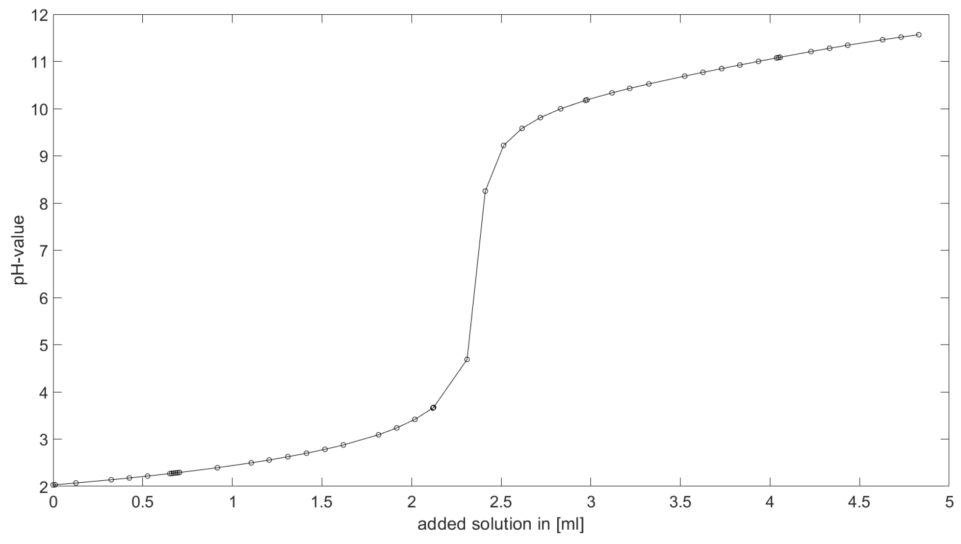
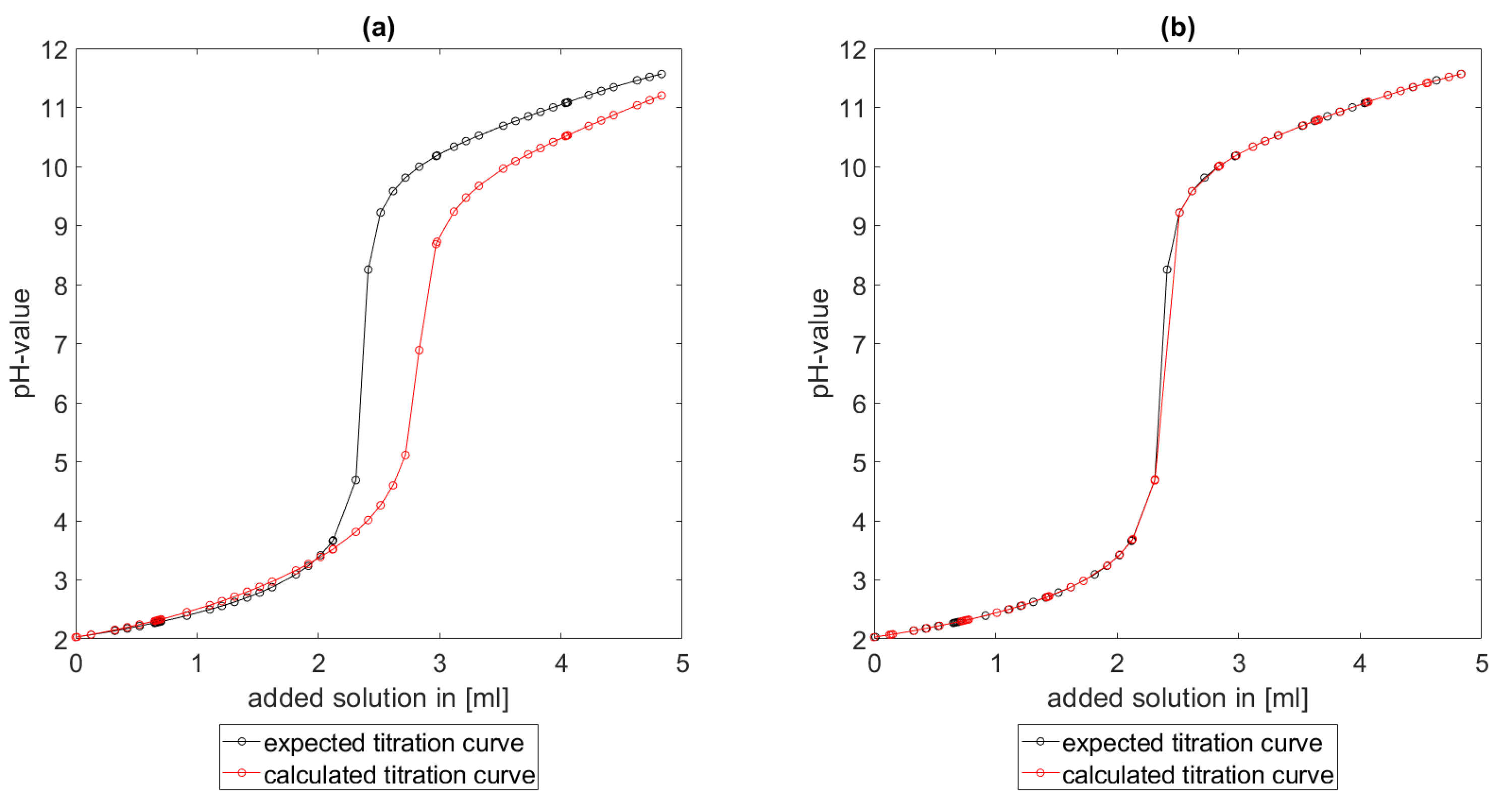
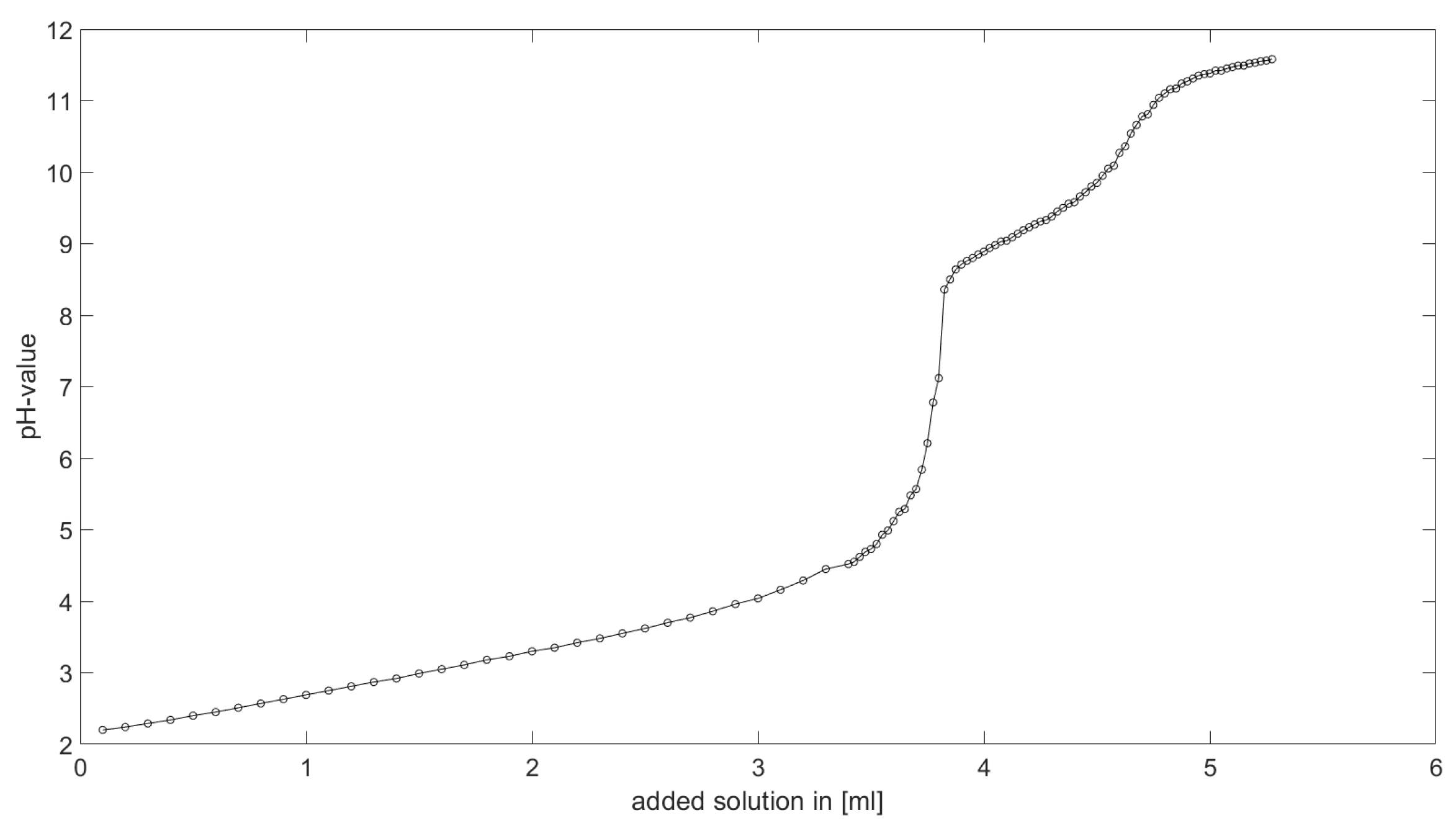
As could be seen from the treatment of the titration of citric acid Cit, see Section 6.1, the measured titration curve is close to the one predicted by the software with stability constants and reactions from literature. Additionally, applying the algorithm for the inverse problem, one observes stability constants close to the values found in the literature.
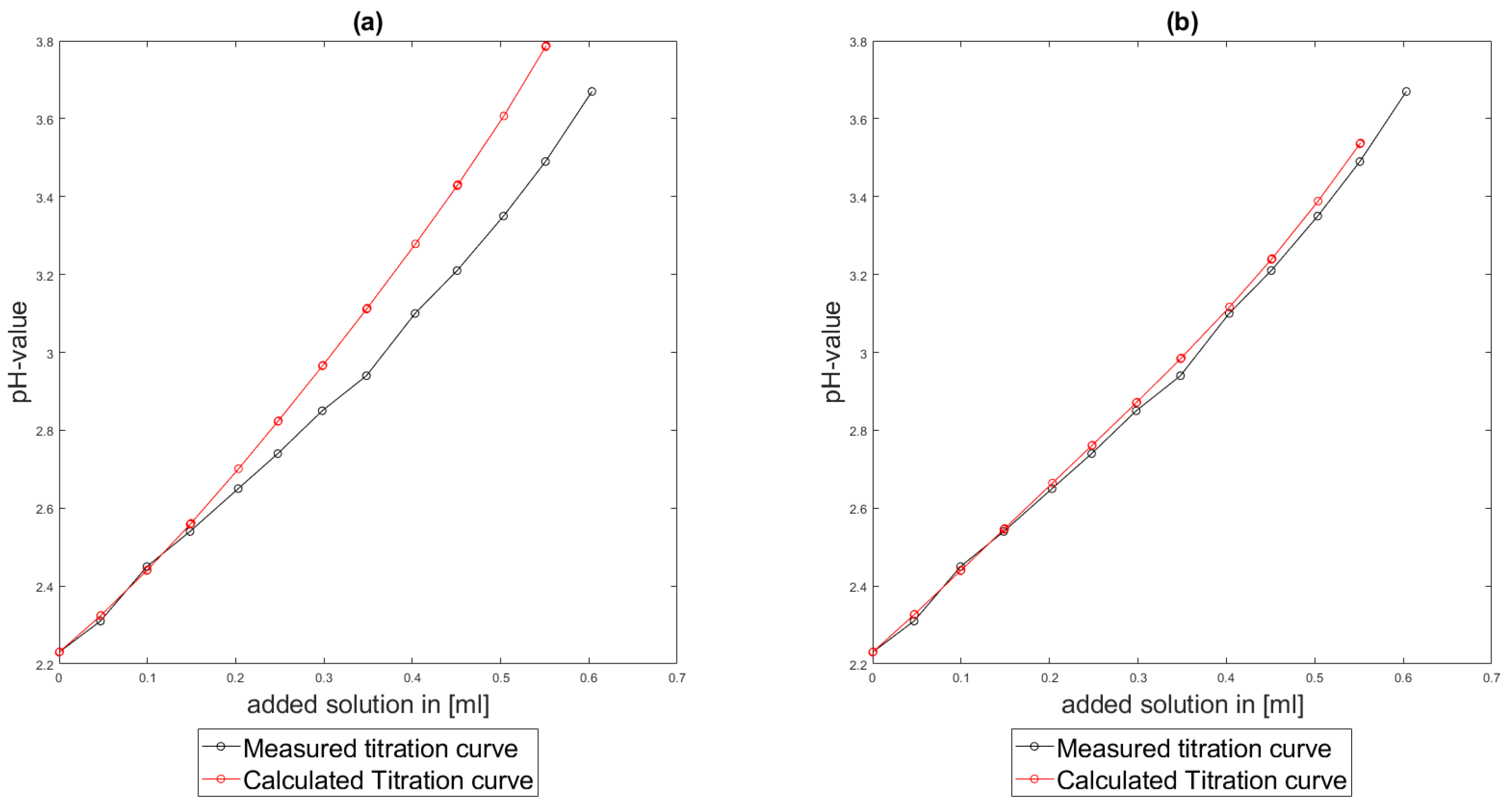
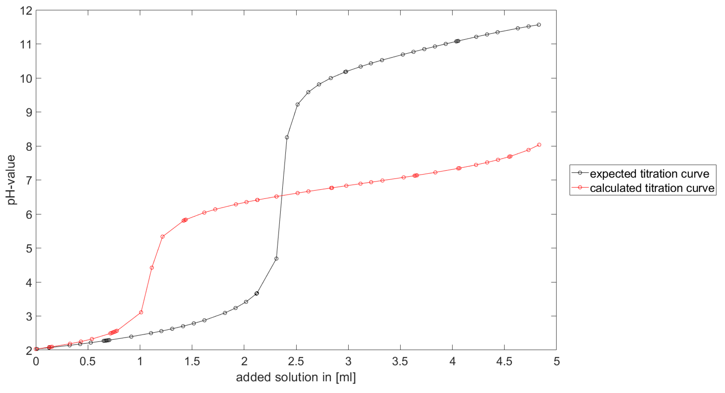
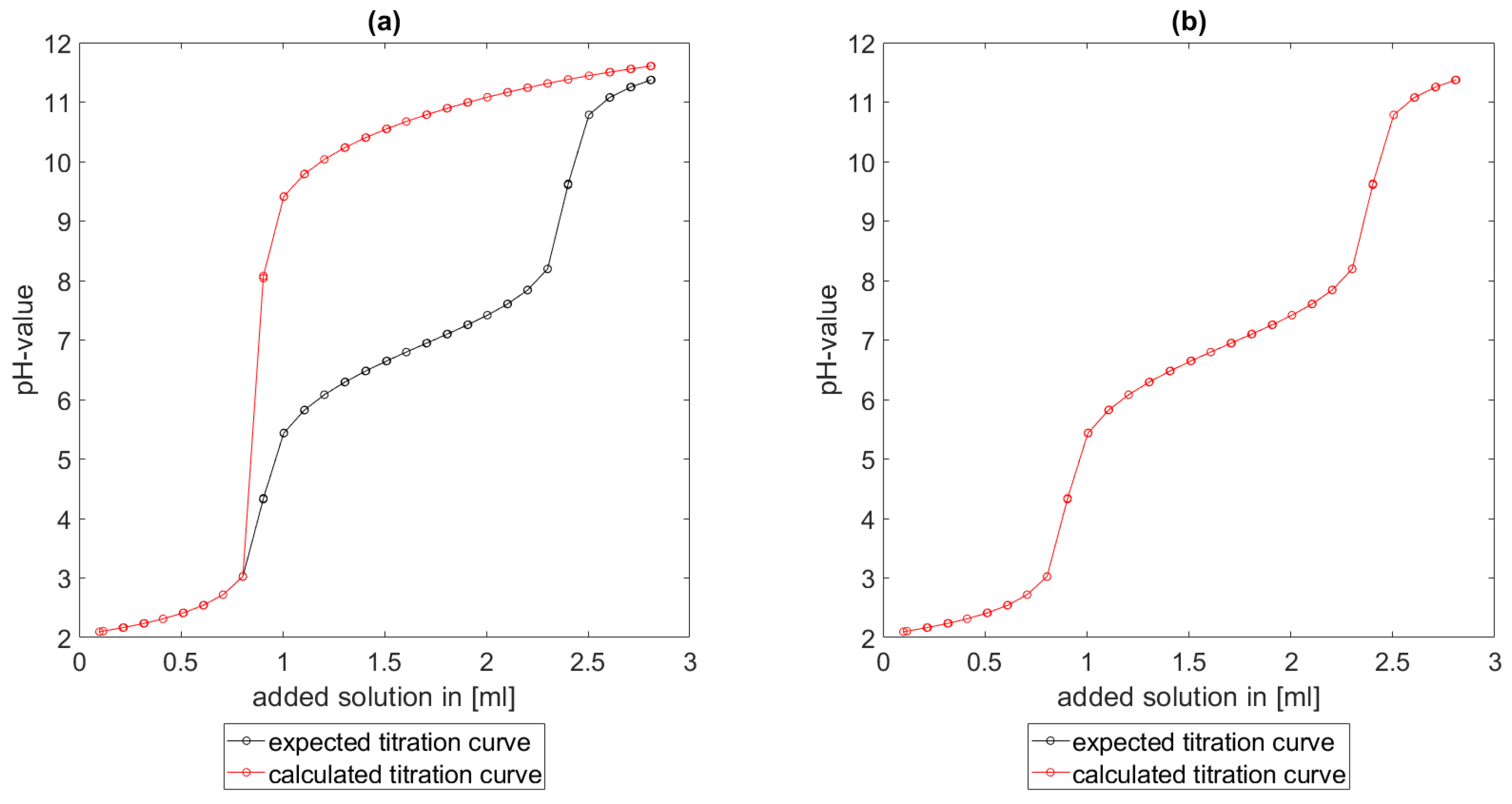
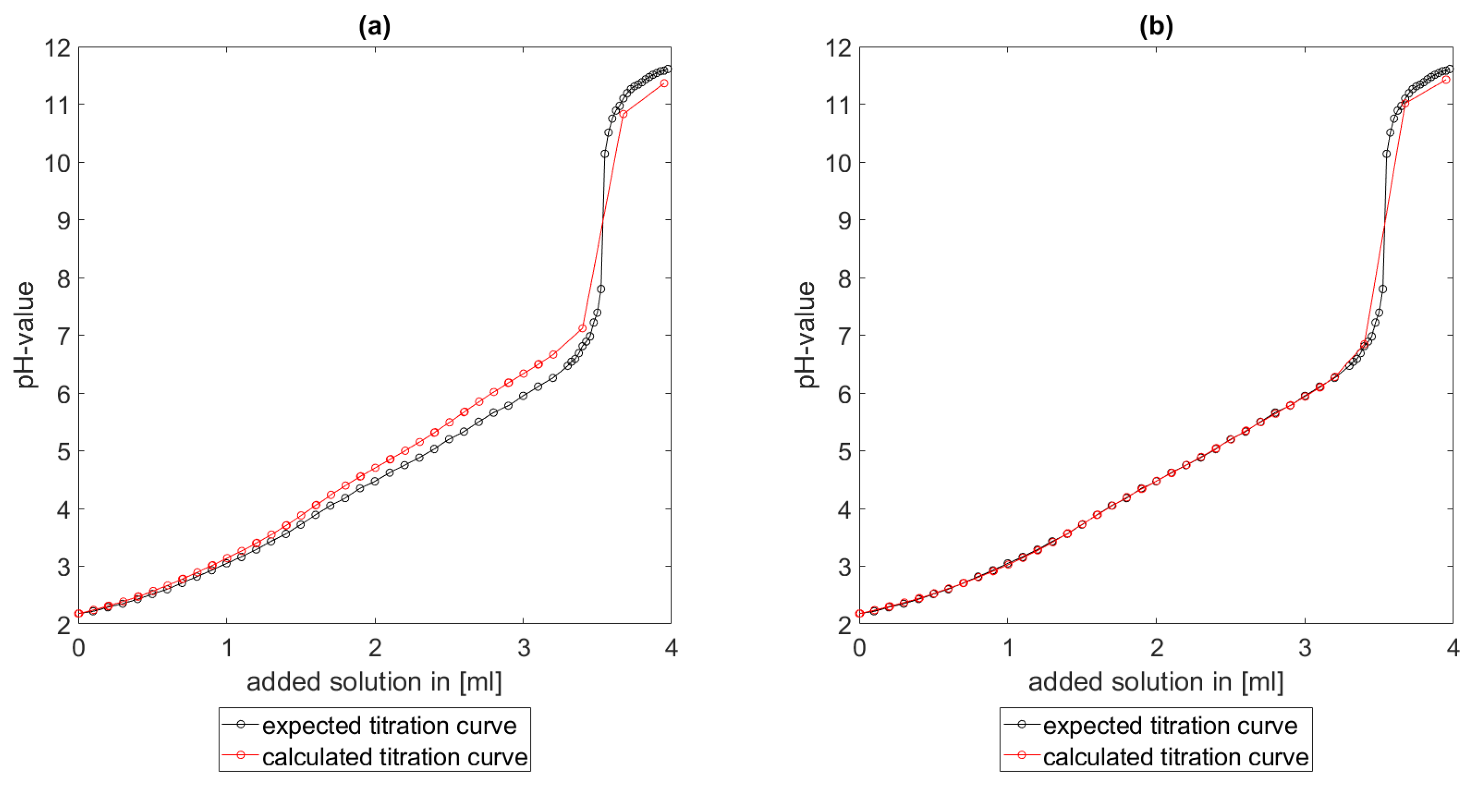
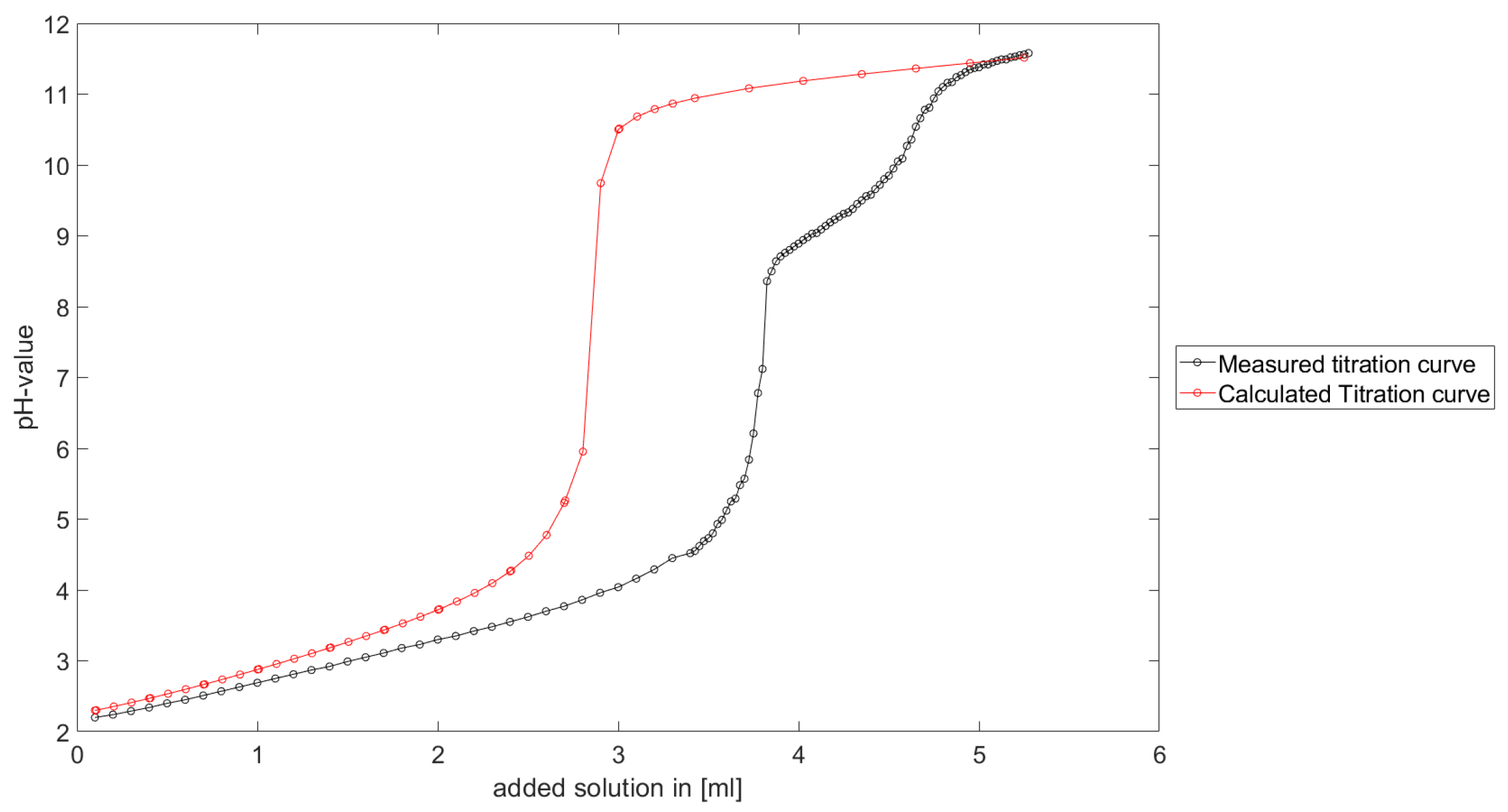
Furthermore, in Section 6.2 and 
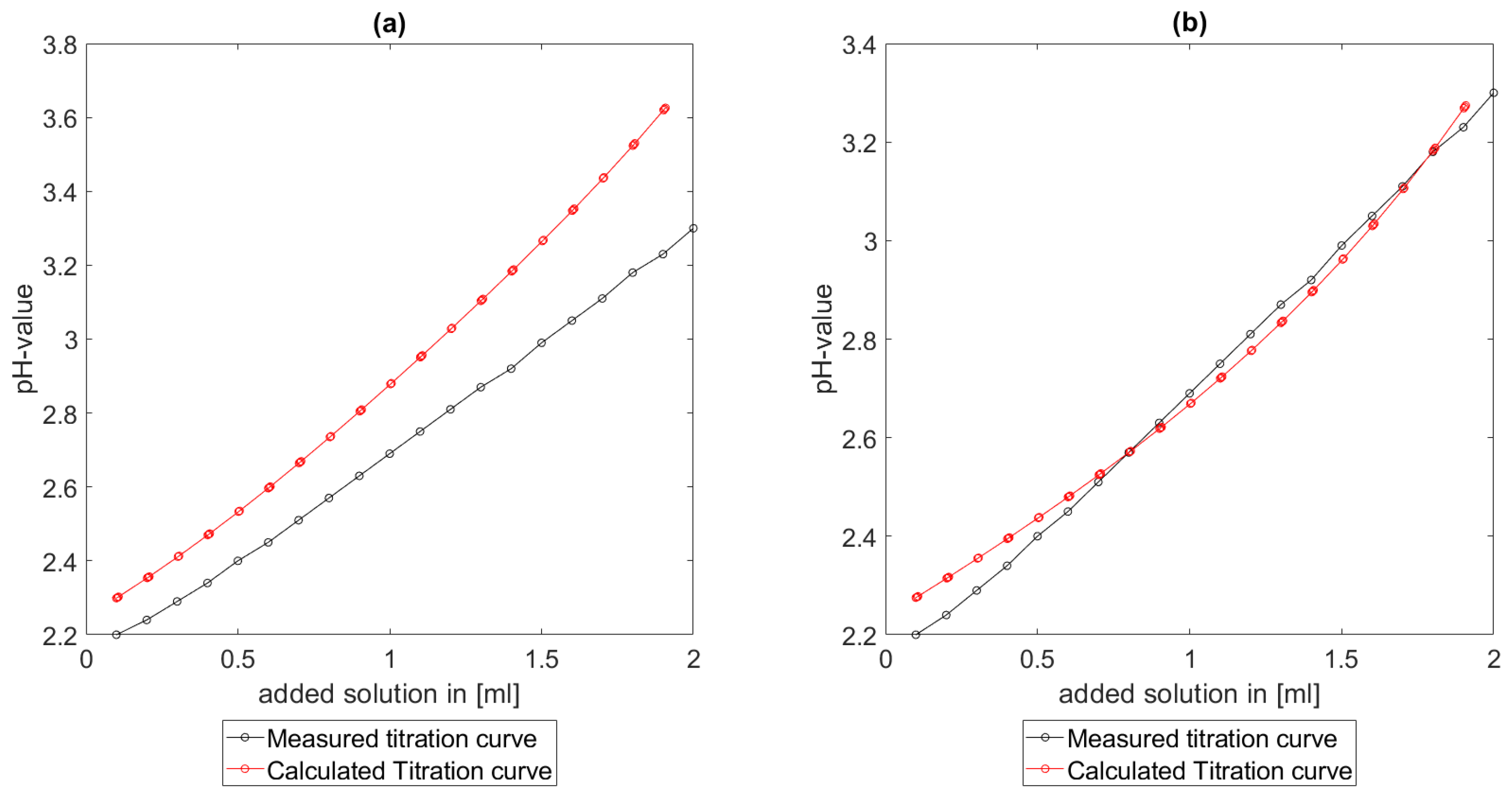
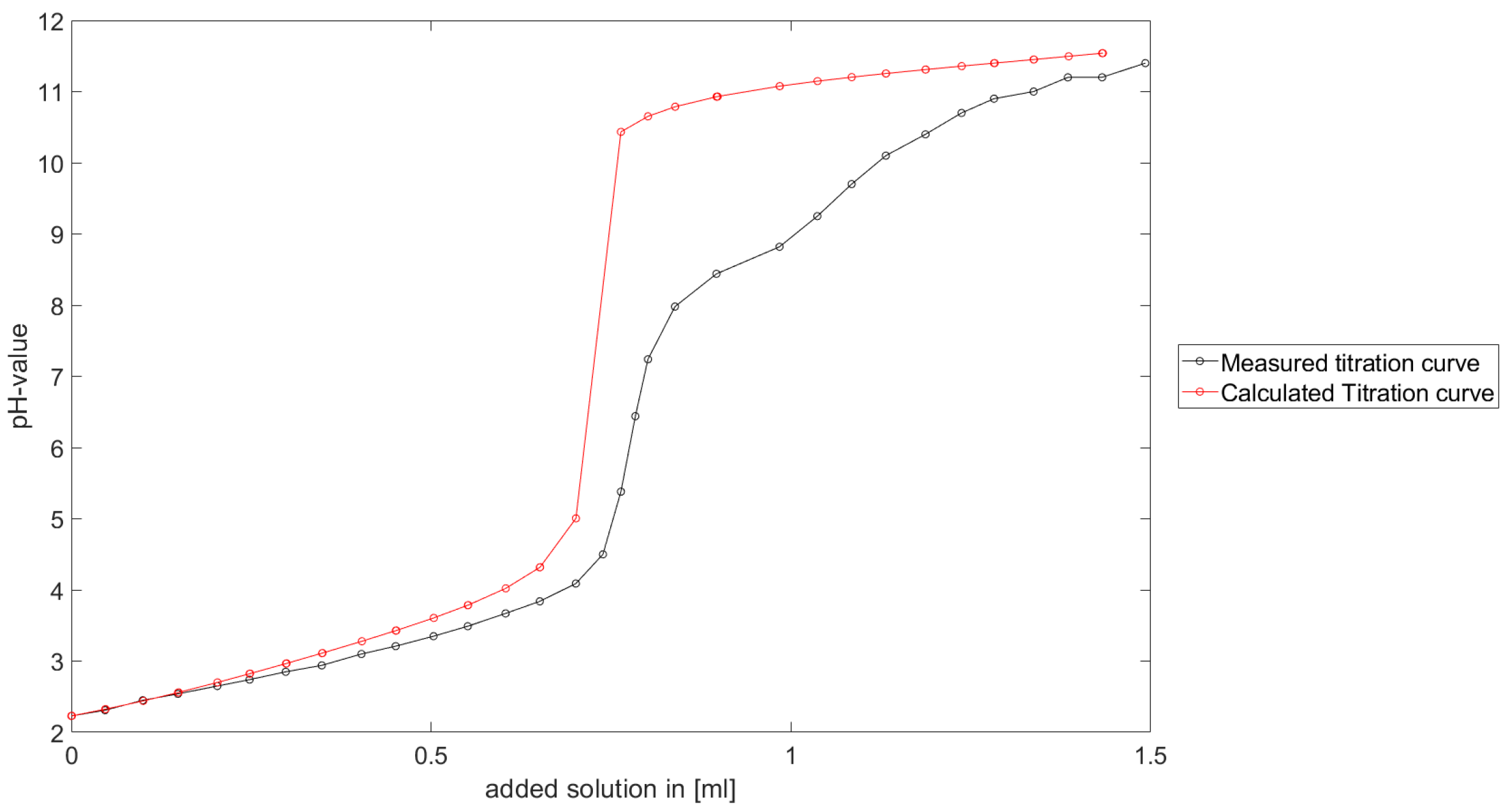
Section 6.3, the software was applied to the titration of a Cit-Ni-electrolyte. In both cases, that of the self-measured titration curve and the one from literature, a gap between the simulated and measured titration curves can be observed. When fitting the whole titration curve, one obtains different stability constants from the values in the literature. However, good agreement between simulated and measured curves is obtained for lower additions and pH values. Satisfactory results of the inverse calculations of the titration curves were obtained.
The behavior discussed above can be explained through the possibility of missing reactions. An error in the software or the general model can be excluded since the simulations in the case of the titration of the Cit-electrolyte and for both Cit-Ni cases for low additions of solutions are plausible, which would not be the case if major mistakes in the modeling or the implementation were done.
Summarizing the results, one obtains a methodology to compute stability constants, which is stable, convergent and guarantees positive stability constants. The computed stability constants are comparable to the results given in the literature. Although the calculated complex formation constants differ from the values in the literature, it is shown that the calculated values are plausible for a significant number of examples. Furthermore, the gap between the measured titration curve and computed titration curve for the Cit-Ni electrolytes indicate some error in the assumed reactions. However, the strength of the methodology described in this article is the adjusted numerical scheme to the experimental setting, in addition to the robustness of the numerical scheme.
For further scientific work besides the identification of stability constants, a study to explain the gap between measurement and simulation is needed. Taking additionally the times of measurements into account the associated kinetic constants of the reactions (2) can be accessible. A further extension of the underlying model on the space component, through diffusion-reaction models, and taking the place of measurement and addition of the titrant, could make diffusion coefficients acceptable.

Author Contributions

Conceptualization, D.H., T.M., T.L. and S.D.S.; methodology, D.H. and S.D.S.; software, S.D.S.; validation, D.H., S.D.S., T.M.; formal analysis, S.D.S.; investigation, D.H. and S.D.S.; resources, D.H.; data curation, D.H. and S.D.S.; writing–original draft preparation, S.D.S. and T.M.; writing–review and editing, T.M. and T.L.; visualization, S.D.S.; supervision, T.M. and T.L.; project administration, S.D.S.; funding acquisition, T.L. All authors have read and agreed to the published version of the manuscript.

Funding

The publication of this article was funded by Chemnitz University of Technology.

Institutional Review Board Statement

Not applicable.

Informed Consent Statement

Not applicable.

Data Availability Statement

The data presented in this study are available on request from thecorresponding author.

Acknowledgments

The authors want to thank E. Schmiedl who programmed first scripts which were important for the intelligent titration and I. Scharf who first initialized the project. Furthermore, the authors want to thank Morgan Uland for English spelling and grammar correction.

Conflicts of Interest

The authors declare no conflict of interest.

Appendix A. The Standard Newtonian Scheme

Let f C 1 ( R d , R d ) be a given continuous and once differentiable function. Furthermore, let f denote the Jacobian matrix of f, then the standard Newtonian scheme is given by the following update rule for each k N
x k : = x k 1 f ( x k 1 ) 1 f ( x k 1 ) .
The corresponding algorithm is assembled in Algorithm A1, see [17].
Algorithm A1: Newtonian Alogorithm
Input: Inital value x 0 R d , tolerance 0 < ε , maximal number of iterations M and set k = 1 .
Output: Error err : = f ( x k ) and approximate solution x k .
Follow the following steps:
S 1
Define x k + 1 with the update rule given by the update rule (A1).
S 2
If f ( x k ) < ε or k = M break the algorithm. Else set k = k + 1 and go to S 1.

References

  1. Dumpala, R.; Srivastava, A.; Rawat, N. Experimental and theoretical approach to probe the aquatic speciation of transuranic (neptunyl) ion in presence of two omnipresent organic moieties. Chemosphere 2021, 273. [Google Scholar] [CrossRef] [PubMed]
  2. Mahmoud, S.; Taha, M.; Mohamed, R.; Khaled, E.; Abdel-khalek, A. Complexation of chromium (III) with the antifibrinolytic drug tranexamic acid: Formation, kinetics, and molecular modeling studies. J. Mol. Liq. 2021, 329. [Google Scholar] [CrossRef]
  3. Cesiulis, H.; Budreika, A. Electroreduction of Ni (II) and Co (II) from Pyrophosphate Solutions. Medziagotyra 2010, 16, 52–56. [Google Scholar]
  4. Schwoebel, S.D.; Mehner, T.; Lampke, T. On a Robust and Efficient Numerical Scheme for the Simulation of Stationary 3-Component Systems with Non-Negative Species-Concentration with an Application to the Cu Deposition from a Cu-(β-alanine)-Electrolyte. Algorithms 2021, 14, 113. [Google Scholar] [CrossRef]
  5. Averós, J.; Llorens, J.; Uribe-Kaffure, R. Numerical simulation of non-linear models of reaction-diffusion for a DGT sensor. Algorithms 2020, 13, 98. [Google Scholar] [CrossRef] [Green Version]
  6. Mongin, S.; Uribe, R.; Puy, J.; Cecília, J.; Galceran, J.; Zhang, H.; Davison, W. Key Role of the Resin Layer Thickness in the Lability of Complexes Measured by DGT. Environ. Sci. Technol. 2011, 45, 4869–4875. [Google Scholar] [CrossRef] [PubMed]
  7. Green, T.A.; Roy, S. Application of a duplex diffusion layer model to pulse reverse plating. Trans. IMF 2017, 95, 46–51. [Google Scholar] [CrossRef] [Green Version]
  8. Xu, L.; Pu, N.; Ye, G.; Xu, C.; Chen, J.; Zhang, X.; Lei, L.; Xiao, C. Unraveling the complexation mechanism of actinide(iii) and lanthanide(iii) with a new tetradentate phenanthroline-derived phosphonate ligand. Inorg. Chem. Front. 2020, 7, 1726–1740. [Google Scholar] [CrossRef]
  9. Luigi Zanonato, P.; Di Bernardo, P.; Melchior, A.; Busato, M.; Tolazzi, M. Lanthanides(III) and Silver(I) complex formation with triamines in DMSO: The effect of ligand cyclization. Inorganica Chim. Acta 2020, 503, 119392. [Google Scholar] [CrossRef]
  10. Becke, A.D. Density-functional exchange-energy approximation with correct asymptotic behavior. Phys. Rev. A 1988, 38, 3098–3100. [Google Scholar] [CrossRef] [PubMed]
  11. Alderighi, L.; Gans, P.; Ienco, A.; Peters, D.; Sabatini, A.; Vacca, A. Hyperquad simulation and speciation (HySS): A utility program for the investigation of equilibria involving soluble and partially soluble species. Coord. Chem. Rev. 1999, 184, 311–318. [Google Scholar] [CrossRef]
  12. Gans, P.; Sabatini, A.; Vacca, A. Investigation of equilibria in solution. Determination of equilibrium constants with the HYPERQUAD suite of programs. Talanta 1996, 43, 1739–1753. [Google Scholar] [CrossRef]
  13. Hinze, P.; Pimau, R.; Ulbrich, M.; Ulbrich, S. Optimization with PDE Constraints, 1st ed.; Mathematical Modelling: Theory and Applications; Springer: Berlin, Germany, 2009; Volume 23. [Google Scholar]
  14. Richter, M. Inverse Probleme-Grundlagen, Theorie und Anwendungsbeispiele, 1st ed.; Springer: Heidelberg/Berlin, Germany, 2015. [Google Scholar]
  15. Langtangen, H.P.; Pedersen, G.K. Ordinary differential equation models. In Scaling of Differential Equations; Springer International Publishing: Cham, Germany, 2016; pp. 17–68. [Google Scholar] [CrossRef] [Green Version]
  16. Mäkelä, M.; Neittaanmäki, P. Nonsmooth Optimization-Analysis and Algorithms with Applications to Optimal Control, 1st ed.; World Scientific Publishing Co. Pte. Ltd.: Singapore, 1992. [Google Scholar]
  17. Lange, K. Optimization, 2nd ed.; Springer Texts in Statistics; Springer: New York, NY, USA, 2013. [Google Scholar]
  18. Li, T.Y. Homotopy Methods. In Encyclopedia of Applied and Computational Mathematics; Engquist, B., Ed.; Springer: Berlin/Heidelberg, Germany, 2015; pp. 653–656. [Google Scholar] [CrossRef]
  19. Watson, L.T. Globally convergent homotopy methodsGlobally Convergent Homotopy Methods. In Encyclopedia of Optimization; Floudas, C.A., Pardalos, P.M., Eds.; Springer: Boston, MA, USA, 2009; pp. 1272–1277. [Google Scholar] [CrossRef]
  20. Martell, A.M. Determination and Use of Stability Constants, 2nd ed.; VCH Puplishers Inc.: Hoboken, NJ, USA, 1992. [Google Scholar]
  21. Saunders, N.; Miodownik, A. (Eds.) Chapter 3-Basic Thermodynamics. In CALPHAD: Calculation of Phase Diagrams; Pergamon Materials Series; The Japan Institute of Metals: Sendai, Japan, 1998; Volume 1, pp. 33–57. [Google Scholar] [CrossRef]
  22. Afanas’ev, V.N.; Zaitsev, A.A.; Ustinov, A.N.; Golubev, V.A. Theory for the determination of activity coefficients of strong electrolytes with regard to concentration dependence of hydration numbers. J. Chem. Thermodyn. 2009, 41, 155–160. [Google Scholar] [CrossRef]
  23. Vincze, J.; Valiskó, M.; Boda, D. The nonmonotonic concentration dependence of the mean activity coefficient of electrolytes is a result of a balance between solvation and ion-ion correlations. J. Chem. Phys. 2010, 133, 154507. [Google Scholar] [CrossRef] [PubMed] [Green Version]
  24. Karimvand, S.K.; Nguyen, X.A.; Abdollahi, H.; Burns, R.; Clifford, S.; Maeder, M.; McCann, N.; Neuhold, Y.M.; Puxty, G. Activity-based analysis of potentiometric pH titrations. Anal. Chim. Acta 2019, 1075, 49–56. [Google Scholar] [CrossRef] [PubMed]
  25. Bosch, S. Algebra; Springer: Berlin/Heidelberg, Germany, 2009. [Google Scholar] [CrossRef]
  26. Ito, K.; Kunisch, K. The augmented lagrangian method for equality and inequality constraints in hilbert spaces. Math. Program. 1990, 46, 341–360. [Google Scholar] [CrossRef]
  27. Kanzow, C.; Steck, D.; Wachsmuth, D. An Augmented Lagrangian Method for Optimization Problems in Banach Spaces. SIAM J. Control. Optim. 2018, 56, 272–291. [Google Scholar] [CrossRef]
  28. Jahn, J. Introduction to the Theory of Nonlinear Optimization; Springer: Berlin/Heidelberg, Germany, 2007. [Google Scholar] [CrossRef]
  29. Nocedal, J.; Wright, S. Numerical Optimization; Springer: New York, NY, USA, 2006; pp. 270–302. [Google Scholar] [CrossRef]
  30. Polak, E. Unconstrained Optimization. In Optimization: Algorithms and Consistent Approximations; Springer: New York, NY, USA, 1997; pp. 1–166. [Google Scholar] [CrossRef]
  31. Ulbrich, M.; Ulbrich, S. Restringierte Optimierung. In Nichtlineare Optimierung; Springer: Basel, Switzerland, 2012; pp. 89–142. [Google Scholar] [CrossRef]
  32. Byrd, R.H.; Gilbert, J.C.; Nocedal, J. A trust region method based on interior point techniques for nonlinear programming. Math. Program. 2000, 89, 149–185. [Google Scholar] [CrossRef] [Green Version]
  33. Zelenin, O. Interaction of the Ni2+ ion with citric acid in an aqueous solution. Russ. J. Coord. Chem. 2007, 38, 346–350. [Google Scholar] [CrossRef]
  34. Orlov, Y.F.; Belkina, E. Correlations between the stability constants of metal hydroxo complexes and the solubility products of crystalline hydroxides. Series of the polarizing effect of metal cations. Russ. J. Inorg. Chem. 2011, 56, 975–980. [Google Scholar] [CrossRef]
Figure 1. Schematic layout of the system for potentiometric titration (1: pH probe, 2: pH meter, 3: capillary for dosing, 4: dosing pump, 5: argon inlet, 6: thermostat bath, 7: magnetic stirrer, 8: PC for data processing).
Computation 09 00055 g001
Figure 2. Example of a titration curve and detailed representation of the pH curve with time units and corresponding base dosing points.
Computation 09 00055 g002
Figure 3. Calculated titration curve with the model associated with the complexes and stability constants as described in Table 1.
Computation 09 00055 g003
Figure 4. (a) Comparison of the initial titration curve regarding parameters in Table 2, (b) Comparison of the optimized titration curve with the initial titration curve; the resulting stability constants can be found in Table 2.
Computation 09 00055 g004
Figure 5. Titration curve with full (black), see Table 1, and reduced system of reactions (red), see Table 3.
Computation 09 00055 g005
Figure 6. Calculated titration curve with complexes and stability constants as defined in Table 4.
Computation 09 00055 g006
Figure 7. (a) Comparison of original titration curve and calculated titration curves with initial stability constants defined in Table 5. (b) Comparison of titration curves with optimized and original stability constants. Numeric results are in Table 5.
Computation 09 00055 g007
Figure 8. Experimentally determined titration curve for citric acid.
Computation 09 00055 g008
Figure 9. (a) Comparison of a measured titration curve and a titration curve calculated from literature data, see Table 6. (b) Comparison of optimized titration curve and measured titration curve. The results of optimization are given in Table 6.
Computation 09 00055 g009
Figure 10. Experimentally determined titration curve for the Cit-Ni electrolyte.
Computation 09 00055 g010
Figure 11. Comparison of a calculated titration curve of the Cit-Ni electrolyte, with literature parameters given in Table 7, and measured Cit-Ni titration curve.
Computation 09 00055 g011
Figure 12. (a) Comparison of calculated titration curve, for the Cit-Ni electrolyte, with stability constants given in the literature, see Figure 7 and measured titration curve on a reduced addition interval. (b) Comparison of measured and optimized titration curves, for the Cit-Ni electrolyte on a reduced addition interval. The results of the optimization are found in Table 7.
Computation 09 00055 g012
Figure 13. Given titration curve for a Cit-Ni electrolyte, from [33].
Computation 09 00055 g013
Figure 14. Comparison of the expected titration curve and the calculated titration curve for a Cit-Ni electrolyte, with stability constants from literature, c.f., Table 8.
Computation 09 00055 g014
Figure 15. (a) Comparison of predicted, with parameters given in Table 8, and expected Cit-Ni titration curve calculated titration curves, for the given Cit-Ni electrolyte. (b) Comparison of expected and optimized titration curves. The results of the optimization can be found in Table 8.
Computation 09 00055 g015
Table 1. Complexes for the software test with moderate stability constants.
ComplexStability Constant log 10 β
1 L 0 M 1 H 0 ( OH ) 7
1 L 0 M 2 H 0 ( OH ) 8
0 L 1 M 0 H 1 ( OH ) 7
0 L 1 M 0 H 2 ( OH ) 8
0 L 1 M 0 H 2 ( OH ) 9
1 L 1 M 0 H 0 ( OH ) 7
2 L 1 M 0 H 0 ( OH ) 8
1 L 1 M 0 H 1 ( OH ) 9
1 L 1 M 0 H 2 ( OH ) 10
0 L 0 M 1 H 1 ( OH ) 15.5148
Table 2. Decadic logarithms of the results of the exact values, initial values, and optimal values.
ComplexExact Stability ConstantInital Value β Optimal Value
1 L 0 M 1 H 0 ( OH ) 78 7.0097
1 L 0 M 2 H 0 ( OH ) 89 7.9951
0 L 1 M 0 H 1 ( OH ) 78 6.9916
0 L 1 M 0 H 2 ( OH ) 89 7.9598
0 L 1 M 0 H 2 ( OH ) 910 9.1193
1 L 1 M 0 H 0 ( OH ) 7--
2 L 1 M 0 H 0 ( OH ) 8--
1 L 1 M 0 H 1 ( OH ) 9--
1 L 1 M 0 H 2 ( OH ) 10--
0 L 0 M 1 H 1 ( OH ) 15.5148 --
Table 3. Decadic logarithms of stability constants for the reduced reaction system.
ComplexStability Constant log 10 β
1 L 0 M 1 H 0 ( OH ) 7
1 L 0 M 2 H 0 ( OH ) 8
0 L 1 M 0 H 1 ( OH ) 7
0 L 1 M 0 H 2 ( OH ) 8
0 L 1 M 0 H 3 ( OH ) 9
0 L 0 M 1 H 1 ( OH ) 15.5148
Table 4. Reaction system with extreme stability constants in decadic logarithms.
ComplexStability Constant
1 L 0 M 1 H 0 ( OH ) 45
0 L 1 M 0 H 1 ( OH ) 50
1 L 1 M 0 H 0 ( OH ) 45
0 L 0 M 1 H 1 ( OH ) 15.5148
Table 5. Results of optimization of the example defined in Table 4. Data given as log 10 β .
ComplexEx. Stab. ConstantInital ValuesOptimal Values
1 L 0 M 1 H 0 ( OH ) 45 42 42
0 L 1 M 0 H 1 ( OH ) 5048 49.9774
1 L 1 M 0 H 0 ( OH ) 4547 44.9782
0 L 0 M 1 H 1 ( OH ) 15.5148 --
Table 6. Results of optimization given for the titration curve given in Figure 8. Values given as log 10 β .
ComplexValues in the literatureOptimal Values
1 L 1 H 0 ( OH ) 6.4 5.8931
1 L 2 H 0 ( OH ) 11.19 10.3762
1 L 3 H 0 ( OH ) 14.33 13.2833
0 L 1 H 1 ( OH ) 15.5343 15.5426
Table 7. Results of optimization of the example defined in Table 4. Data given as log 10 β .
ComplexValues in the literatureOptimal Values
1 L 0 M 1 H 0 ( OH ) 6.4 5.9723
1 L 0 M 2 H 0 ( OH ) 11.19 10.4553
1 L 0 M 3 H 0 ( OH ) 14.33 13.1864
1 L 1 M 0 H 0 ( OH ) 6.86 7.0568
1 L 1 M 1 H 0 ( OH ) 10.58 10.4057
1 L 1 M 2 H 0 ( OH ) 13.43 11.624
0 L 1 M 0 H 1 ( OH ) 4.4 4.40001
0 L 0 M 0 H 2 ( OH ) 9 8.9999
0 L 1 M 0 H 3 ( OH ) 12 11.9999
0 L 1 M 0 H 4 ( OH ) 12 11.9999
0 L 0 M 1 H 1 ( OH ) 15.5343 15.5426
Table 8. Results of optimization of the example defined in Table 4. Data given as log 10 β .
ComplexValues in the literatureOptimal Values
1 L 0 M 1 H 0 ( OH ) 6.4 5.9622
1 L 0 M 2 H 0 ( OH ) 11.19 10.2793
1 L 0 M 3 H 0 ( OH ) 14.33 13.3625
1 L 1 M 0 H 0 ( OH ) 6.86 6.0180
1 L 1 M 1 H 0 ( OH ) 10.58 9.8144
1 L 1 M 2 H 0 ( OH ) 13.43 11.8669
0 L 1 M 0 H 1 ( OH ) 4.4 4.401
0 L 0 M 0 H 2 ( OH ) 9 9.0009
0 L 1 M 0 H 3 ( OH ) 12 12.0041
0 L 1 M 0 H 4 ( OH ) 12 12.013
0 L 0 M 1 H 1 ( OH ) 15.5343 15.54299
Publisher’s Note: MDPI stays neutral with regard to jurisdictional claims in published maps and institutional affiliations.

