Article

Hybrid Feedback Control for Exponential Stability and Robust H Control of a Class of Uncertain Neural Network with Mixed Interval and Distributed Time-Varying Delays

1
Department of Mathematics, Faculty of Science, Khon Kaen University, Khon Kaen 40002, Thailand
2
Department of Mathematics, Faculty of Science, University of Phayao, Phayao 56000, Thailand
3
Department of Mathematics Statistics and Computer, Faculty of Science, Ubon Ratchathani University, Ubon Ratchathani 34190, Thailand
*
Authors to whom correspondence should be addressed.
Submission received: 29 April 2021 / Revised: 19 May 2021 / Accepted: 25 May 2021 / Published: 28 May 2021

Abstract

:
This paper is concerned the problem of robust H control for uncertain neural networks with mixed time-varying delays comprising different interval and distributed time-varying delays via hybrid feedback control. The interval and distributed time-varying delays are not necessary to be differentiable. The main purpose of this research is to estimate robust exponential stability of uncertain neural network with H performance attenuation level γ . The key features of the approach include the introduction of a new Lyapunov–Krasovskii functional (LKF) with triple integral terms, the employment of a tighter bounding technique, some slack matrices and newly introduced convex combination condition in the calculation, improved delay-dependent sufficient conditions for the robust H control with exponential stability of the system are obtained in terms of linear matrix inequalities (LMIs). The results of this paper complement the previously known ones. Finally, a numerical example is presented to show the effectiveness of the proposed methods.

1. Introduction

During the past decades, the problem of the reliable control has received much attention [1,2,3,4,5,6,7,8,9,10,11]. Neural networks have received considerable due to the effective use of many aspects such as signal processing, automatic control engineering, associative memories, parallel computation, fault diagnosis, combinatorial optimization and pattern recognition and so on [12,13,14]. It has been shown that the presence of time delay in a dynamical system is often a primary source of instability and performance degradation [15]. Many researchers have paid attentions to the problem of robust stability for uncertain systems with time delays [16,17,18,19]. The H controller can be used to guarantee closed loop system not only a robust stability but also an adequate level of performance. In practical control systems, actuator faults, sensor faults or some component faults may happen, which often lead to unsatisfactory performance, even loss of stability. Therefore, research on reliable control is necessary.
On the other hand, the H control of time-delay systems are practical and theoretical interest since time delay is often encountered in many engineering and industrial processes [20,21,22].
Most of works have been focused on the problem of designing a robust H controller that stabilizes linear uncertain systems with time-varying norm bounded parameter uncertainty in the state and input matrices. The problem of designing a robust reliable H controller for neural networks is considered in [23]. Ref [24] have studied the problem of delay dependent robust H control for a class of uncertain systems with distributed time-varying delays. The parameter uncertainties are supposed to be time-varying and norm bounded. The problem of H control design usually leads to solving an algebraic Lyaponov equation. It should be noted that some works have been dedicated to the problem of robust reliable control for nonlinear systems with time-varying delay [2,4,7]. However, to the best of the authors’s knowledge, so far the research on robust reliable H control is still open problems, which are worth further investigations.
Motivated by above discussion, in this paper we have considered the problem of a robust H control for a class of uncertain systems with interval and distributed time-varying delays. The parameter uncertainties are supposed to be time varying and norm bounded. A sufficient condition for the H control is presented by LMIs approach using a new LKF with triple integral terms. The robust exponential stability of the system is established which satisfy a formulated H performance level for all admissible parameters uncertainties.
The main contributions of this paper are given as follows,
  • This research is the first time to study hybrid feedback control for exponential stability and robust H control of a class of uncertain neural network with mixed interval and distributed time-varying delays.
  • A novel LKF V 1 ( t , x t ) = x T ( t ) P 1 x ( t ) + 2 x T ( t ) P 2 t h 2 t x ( s ) d s + t h 2 t x ( s ) d s T × P 3 t h 2 t x ( s ) d s + 2 x T ( t ) P 4 h 2 0 t + s t x ( θ ) d θ d s + 2 t h 2 t x ( s ) d s T × P 5 h 2 0 t + s t x ( θ ) d θ d s + h 2 0 t + s t x ( θ ) d θ d s T P 6 h 2 0 t + s t x ( θ ) d θ d s is first proposed to analyze the problem of robust H control for uncertain neural networks with mixed time-varying delays and augmented Lyapunov matrix P i ( i = 1 , 2 , , 6 ) do not need to be positive definiteness of the chosen LKF compared with [23].
  • The problem of robust H control for uncertain neural networks with mixed time-varying delays comprising of interval and distributed time-varying delays, these delays are not necessarily differentiable.
  • For the neural networks system (1), the output z ( t ) contains the deterministic disturbance input w ( t ) and the feedback control u ( t ) which is more general and applicable than [23,24,25,26,27,28].
The rest of this paper is organized as follows. In Section 2, some notations, definitions and some well-known technical lemmas are given. Section 3 presents the H control for exponential stability and the robust H control for exponential stability. The numerical examples and their computer simulations are provided in Section 4 to indicate the effectiveness of the proposed criteria. Finally, this paper is concluded in Section 5.

2. Model Description and Mathematic Preliminaries

The following notation will be used in this paper: R and R + denote the set of real numbers and the set of nonnegative real numbers, respectively. R n denotes the n dimensional space. R n × r denotes the set of n × r real matrices. C [ [ ϱ , 0 ] , R n ] denotes the space of all continuous vector functions mapping [ ϱ , 0 ] into R n where ϱ R + . A T and A 1 denote the transpose and the inverse of matrix A, respectively. A is symmetric if A = A T , λ ( A ) denotes all the eigenvalue of A, λ max ( A ) = max { R e λ : λ λ ( A ) } , λ min ( A ) = min { R e λ : λ λ ( A ) } , A > 0 or A < 0 denotes that the matrix A is a symmetric and positive definite or negative definite matrix. If A , B are symmetric matrices, A > B means that A B is positive definite matrix, I denotes the identity matrix with appropriate dimensions. The symmetric term in the matrix is denoted by *. The following norms will be used: | | · | | refer to the Euclidean vector norm; | | ϕ | | c = sup t [ ϱ , 0 ] | | ϕ ( t ) | | stands for the norm of a function ϕ ( · ) C [ [ ϱ , 0 ] , R n ] .
Consider the following neural network system with mixed time delays
x ˙ ( t ) = A x ( t ) + B f ( x ( t ) ) + C g ( x ( t h ( t ) ) ) + D t d ( t ) t h ( x ( s ) ) d s + E w ( t ) + U ( t ) , z ( t ) = A 1 x ( t ) + B 4 x ( t h ( t ) ) + C 1 u ( t ) + D 1 t d ( t ) t x ( s ) d s + E 1 w ( t ) , x ( t ) = ϕ ( t ) , t [ ϱ , 0 ] ,
where x ( t ) R n is the state vector, w ( t ) R n the deterministic disturbance input, z ( t ) R n the system output, f ( x ( t ) ) , g ( x ( t ) ) , h ( x ( t ) ) the neuron activation function, A = d i a g { a 1 , , a n } > 0 is a diagonal matrix, B , C , D , E , A 1 , B 4 , C 1 , D 1 , E 1 are the known real constant matrices with appropriate dimensions, ϕ ( t ) C [ [ ϱ , 0 ] , R n ] the initial function, The state hybrid feedback controller U ( t ) satisfies:
U ( t ) = B 1 u ( t ) + B 2 u ( t τ ( t ) ) + B 3 t d 1 ( t ) t u ( s ) d s ,
where u ( t ) = K x ( t ) and K is a constant matrix control gain, B 1 , B 2 , B 3 are the known real constant matrices with appropriate dimensions. Then, substituting it into (1), it is easy to get the following:
x ˙ ( t ) = [ A + B 1 K ] x ( t ) + B f ( x ( t ) ) + C g ( x ( t h ( t ) ) ) + D t d ( t ) t h ( x ( s ) ) d s + E w ( t ) + B 2 K x ( t τ ( t ) ) + B 3 K t d 1 ( t ) t x ( s ) d s , z ( t ) = [ A 1 + C 1 K ] x ( t ) + B 4 x ( t h ( t ) ) + D 1 t d ( t ) t x ( s ) d s + E 1 w ( t ) , x ( t ) = ϕ ( t ) , t [ ϱ , 0 ] ,
where the time-varying delays function h ( t ) , τ ( t ) , d ( t ) and d 1 ( t ) satisfy the condition
0 h 1 h ( t ) h 2 , 0 d ( t ) d , 0 τ ( t ) τ , 0 d 1 ( t ) d 1 ,
where h 1 , h 2 , τ , d, d 1 , ϱ = max { h 2 , τ , d , d 1 } are real constant scalars and we denote h 12 = h 2 h 1 .
Throughout this paper, we consider activation functions f ( · ) , g ( · ) and h ( · ) satisfy Lipschitzian with the Lipschitz constants f ^ i , g ^ i and h ^ i > 0 :
| f i ( x 1 ) f i ( x 2 ) | f ^ i | x 1 x 2 | , | g i ( x 1 ) g i ( x 2 ) | g ^ i | x 1 x 2 | , | h i ( x 1 ) h i ( x 2 ) | h ^ i | x 1 x 2 | ,
where i = 1 , 2 , , n , x 1 , x 2 R and we denote that
F = d i a g { f ^ i , i = 1 , 2 , , n } , G = d i a g { g ^ i , i = 1 , 2 , , n } , H = d i a g { h ^ i , i = 1 , 2 , , n } .
Remark 1.
If B 2 = 0 , B 3 = 0 , B 4 = 0 , D 1 = 0 , E 1 = 0 , and f ( · ) = g ( · ) = h ( · ) , the system (3) turns into the neural network with activation functions and time-varying delays proposed by [23]
x ˙ ( t ) = [ A + B 1 K ] x ( t ) + B f ( x ( t ) ) + C f ( x ( t h ( t ) ) ) + D t d ( t ) t f ( x ( s ) ) d s + E w ( t ) , z ( t ) = [ A 1 + C 1 K ] x ( t ) , x ( t ) = ϕ ( t ) , t [ ϱ , 0 ] .
Hence, the system (3) is general neural networks model, with (7) as the special case.
The following definition and lemma are necessary in the proof of the main results:
Definition 1
([29]). Given α > 0 . The zero solution of system (1), where u ( t ) = 0 , w ( t ) = 0 , is α stable if there is a positive number N > 0 such that every solution of the system satisfies
| | x ( t , ϕ ) | | N | | ϕ | | c e α t , t 0 .
Definition 2
([29]). Consider α > 0 and γ > 0 . The H control problem for system (1) has a solution if there exists a memoryless state feedback controller u ( t ) = K x ( t ) satisfying the following two requirements:
(i) 
The zero solution of the closed-loop system, where w ( t ) = 0 ,
x ˙ ( t ) = A x ( t ) + B f ( x ( t ) ) + C g ( x ( t h ( t ) ) ) + D t d ( t ) t h ( x ( s ) ) d s + U ( t ) , is α stable.
(ii) 
There is a number c 0 > 0 such that
sup 0 | | z ( t ) | | 2 d t c 0 | | ϕ | | c 2 + 0 | | w ( t ) | | 2 d t γ ,
where the supremum is taken over all ϕ ( t ) C [ [ ϱ , 0 ] , R n ] and the non-zero uncertainty w ( t ) L 2 ( [ 0 , ] , R n ) .
Lemma 1
([30], Cauchy inequality). For any symmetric positive definite matrix N M n × n and x , y R n we have
± 2 x T y x T N x + y T N 1 y .
Lemma 2
([30]). For a positive definite matrix Z R n × n , and two scalars 0 r 1 < r 2 and vector function x : [ r 1 , r 2 ] R n such that the following integrals are well defined, one has
r 1 r 2 x ( s ) d s T Z r 1 r 2 x ( s ) d s ( r 2 r 1 ) r 1 r 2 x T ( s ) Z x ( s ) d s .
Lemma 3
([31]). For any positive definite symmetric constant matrix P and scalar τ > 0 , such that the following integrals are well defined, one has
τ 0 t + θ t x T ( s ) P x ( s ) d s d θ 2 τ 2 τ 0 t + θ t x ( s ) d s d θ T P τ 0 t + θ t x ( s ) d s d θ .
Lemma 4
([32]). For given matrices H, E, and F with F T F I and a scalar ϵ > 0 , the following inequality holds:
H F E + ( H F E ) T ϵ H H T + ϵ 1 E T E .

3. Stability Analysis

In this section, we will present stability criterion for system (3).
Consider a Lyapunov–Krasovskii functional candidate as
V ( t , x t ) = i = 1 14 V i ( t , x t ) ,
where
V 1 ( t , x t ) = x T ( t ) P 1 x ( t ) + 2 x T ( t ) P 2 t h 2 t x ( s ) d s + t h 2 t x ( s ) d s T P 3 t h 2 t x ( s ) d s + 2 x T ( t ) P 4 h 2 0 t + s t x ( θ ) d θ d s + 2 t h 2 t x ( s ) d s T P 5 h 2 0 t + s t x ( θ ) d θ d s + h 2 0 t + s t x ( θ ) d θ d s T P 6 h 2 0 t + s t x ( θ ) d θ d s , V 2 ( t , x t ) = t h 1 t e 2 α ( s t ) x T ( s ) R 1 x ( s ) d s , V 3 ( t , x t ) = t h 2 t e 2 α ( s t ) x T ( s ) R 2 x ( s ) d s , V 4 ( t , x t ) = h 1 h 1 0 t + s t e 2 α ( θ t ) x ˙ T ( θ ) Q 1 x ˙ ( θ ) d θ d s , V 5 ( t , x t ) = h 2 h 2 0 t + s t e 2 α ( θ t ) x ˙ T ( θ ) Q 2 x ˙ ( θ ) d θ d s , V 6 ( t , x t ) = h 12 h 2 h 1 t + s t e 2 α ( θ t ) x ˙ T ( θ ) Z 2 x ˙ ( θ ) d θ d s , V 7 ( t , x t ) = d 0 t + s t e 2 α ( θ t ) h T ( x ( θ ) ) U h ( x ( θ ) ) d θ d s , V 8 ( t , x t ) = d 1 0 t + s t e 2 α ( θ t ) u T ( θ ) S 2 u ( θ ) d θ d s , V 9 ( t , x t ) = τ τ 0 t + s t e 2 α ( θ t ) u ˙ T ( θ ) S 1 u ˙ ( θ ) d θ d s , V 10 ( t , x t ) = h 2 h 1 s 0 t + u t e 2 α ( θ + u t ) x ˙ T ( θ ) Z 1 x ˙ ( θ ) d θ d u d s , V 11 ( t , x t ) = h 1 0 τ 0 t + s t e 2 α ( θ + s t ) x ˙ T ( θ ) W 1 x ˙ ( θ ) d θ d s d τ , V 12 ( t , x t ) = h 2 0 τ 0 t + s t e 2 α ( θ + s t ) x ˙ T ( θ ) W 2 x ˙ ( θ ) d θ d s d τ , V 13 ( t , x t ) = h 2 0 τ 0 t + s t e 2 α ( θ + s t ) x ˙ T ( θ ) W 3 x ˙ ( θ ) d θ d s d τ , V 14 ( t , x t ) = d 0 t + s t e 2 α ( θ t ) x T ( θ ) Q 3 x ( θ ) d θ d s .
Remark 2.
Note that the Lyapunov–Krasovskii functional, P i ( i = 1 , 2 , , 6 ) in V 1 ( t , x t ) are not necessary to be positive definite.
Proposition 1.
Given α > 0 , the Lyapunov–Krasovskii functional (8) is positive definite, if there exist matrices P 1 = P 1 T , P 3 = P 3 T , P 6 = P 6 T , P 2 , P 4 , P 5 , Q 1 > 0 , Q 2 > 0 , Q 3 > 0 , R 1 > 0 , R 2 > 0 , S 1 > 0 , S 2 > 0 , U > 0 , W 1 > 0 , W 2 > 0 , W 3 > 0 , Z 1 > 0 , Z 2 > 0 such that the following LMI holds:
Θ = Θ 11 Θ 12 Θ 13 * Θ 22 P 5 * * Θ 33 > 0 ,
where
Θ 11 = P 1 + h 2 e 2 α h 2 Q 2 + 0.5 h 2 e 4 α h 2 W 3 , Θ 12 = P 2 e 2 α h 2 Q 2 ,
Θ 13 = P 4 h 2 1 e 4 α h 2 W 3 ,
Θ 22 = P 3 + h 2 1 e 2 α h 2 ( Q 2 + R 2 ) ,
Θ 33 = P 6 + h 2 3 e 4 α h 2 ( W 3 + W 3 T ) .
Proof. 
Let y 1 ( t ) = t h 2 t x ( s ) d s , y 2 ( t ) = h 2 0 t + s t x ( θ ) d θ d s , then we can get
V 1 ( t , x t ) = x T ( t ) P 1 x ( t ) + 2 x T ( t ) P 2 y 1 ( t ) + y 1 T ( t ) P 3 y 1 ( t ) + 2 x T ( t ) P 4 y 2 ( t ) + 2 y 1 T ( t ) P 5 y 2 ( t ) + y 2 T ( t ) P 6 y 2 ( t ) ,
V 3 ( t , x t ) e 2 α h 2 t h 2 t x T ( s ) R 2 x ( s ) d s = h 2 1 e 2 α h 2 y 1 T ( t ) R 2 y 1 ( t ) ,
V 5 ( t , x t ) h 2 e 2 α h 2 h 2 0 t + s t x ˙ T ( θ ) Q 2 x ˙ ( θ ) d θ d s h 2 e 2 α h 2 h 2 0 s 1 t + s t x ˙ ( θ ) d θ T Q 2 t + s t x ˙ ( θ ) d θ d s e 2 α h 2 h 2 0 [ x ( t ) x ( t + s ) ] T Q 2 [ x ( t ) x ( t + s ) ] d s = x ( t ) y 1 ( t ) T h 2 e 2 α h 2 Q 2 e 2 α h 2 Q 2 * h 2 1 e 2 α h 2 Q 2 x ( t ) y 1 ( t ) ,
V 13 ( t , x t ) e 2 α h 2 h 2 0 τ 0 t + s t x ˙ T ( θ ) W 3 x ˙ ( θ ) d θ d s d τ e 2 α h 2 h 2 0 τ 0 s 1 t + s t x ˙ ( θ ) d θ T W 3 t + s t x ˙ ( θ ) d θ d s d τ h 2 1 e 2 α h 2 h 2 0 τ 0 [ x ( t ) x ( t + s ) ] T W 3 [ x ( t ) x ( t + s ) ] d s d τ = x ( t ) y 2 ( t ) T 0.5 h 2 e 4 α h 2 W 3 h 2 1 e 4 α h 2 W 3 * h 2 3 e 4 α h 2 ( W 3 + W 3 T ) x ( t ) y 2 ( t ) .
Combining with V 2 ( t , x t ) , V 4 ( t , x t ) , V 6 ( t , x t ) V 12 ( t , x t ) , V 14 ( t , x t ) , we know that if the LMI (9) holds, the LKF (8) is positive definite. This completes the proof. □
Let us set
λ 1 = λ min ( P 1 ) , λ 2 = 3 h 2 2 λ max ( Θ ) + h 1 λ max ( R 1 ) + h 1 2 λ max ( Q 1 ) + h 12 2 λ max ( Z 2 ) + d 1 2 λ max ( P 1 1 B 1 T S 2 B 1 P 1 1 ) + τ 2 λ max ( P 1 1 B 1 T S 1 B 1 P 1 1 ) + h 12 h 2 2 λ max ( Z 1 ) + h 1 2 λ max ( W 1 ) + h 2 2 λ max ( W 2 ) + d 2 λ max ( Q 3 ) + d 2 λ max ( H T U H ) .
Remark 3.
It is noted that the previous works [23,24,25,26,27,28] consider the Lyapunov martices P 1 , P 3 and P 6 which are positive definite. In our paper, we remove this restriction by applying the method of constructing complicated Lyapunov V 1 ( t , x t ) , V 3 ( t , x t ) , V 5 ( t , x t ) and V 13 ( t , x t ) as shown in the proof of Proposition 1. Hence, P 1 , P 3 and P 6 are only real matrices. It can be seen that our paper are more applicable and less conservative than aforementioned works.
Theorem 1.
Given α > 0 , The H control of system (3) has a solution if there exist symmetric positive definite matrices Q 1 , Q 2 , Q 3 , R 1 , R 2 , S 1 , S 2 , S 3 , W 1 , W 2 , W 3 , Z 1 , Z 2 , Z 3 , diagonal matrices U > 0 , U 2 > 0 , U 3 > 0 , and matrices P 1 = P 1 T , P 3 = P 3 T , P 6 = P 6 T , P 2 , P 4 , P 5 such that the following LMIs hold:
Ξ 1 = Π F T P 1 P 1 2 d P 1 D 4 P 1 B 2 2 d 1 P 1 B 3 P 1 E * U 2 0 0 0 0 0 * * U 3 0 0 0 0 * * * Ξ 1 ( 4 , 4 ) 0 0 0 * * * * Ξ 1 ( 5 , 5 ) 0 0 * * * * * Ξ 1 ( 6 , 6 ) 0 * * * * * * 0.5 γ < 0 ,
Ξ 2 = 0.4 R 1 R 1 B R 1 C 2 d R 1 D 4 R 1 B 2 2 d 1 R 1 B 3 R 1 B 1 R 1 E * U 2 0 0 0 0 0 0 * * U 3 0 0 0 0 0 * * * Ξ 2 ( 4 , 4 ) 0 0 0 0 * * * * Ξ 2 ( 5 , 5 ) 0 0 0 * * * * * Ξ 2 ( 6 , 6 ) 0 0 * * * * * * S 3 0 * * * * * * * 0.5 γ < 0 ,
Ξ 3 = 0.5 e 2 α h 2 Q 2 + N < 0 ,
Ξ 4 = 0.1 R 1 + τ 2 B 1 T S 1 B 1 < 0 ,
where
Π = Π 1 , 1 Π 1 , 2 0 Π 1 , 4 Π 1 , 5 Π 1 , 6 Π 1 , 7 0 Π 1 , 9 A T R 1 * Π 2 , 2 Π 2 , 3 Π 2 , 4 0 0 0 0 0 0 * * Π 3 , 3 Π 3 , 4 0 0 0 0 0 0 * * * Π 4 , 4 0 P 3 0 0 P 5 0 * * * * Π 5 , 5 0 0 0 0 0 * * * * * Π 6 , 6 0 0 Π 6 , 9 P 2 * * * * * * Π 7 , 7 0 0 0 * * * * * * * Π 8 , 8 0 0 * * * * * * * * 2 α P 6 P 4 * * * * * * * * * Π 10 , 10 < 0 ,
Π 1 , 1 = A P 1 P 1 A T + B 1 B 1 + B 1 T B 1 T + P 2 + P 2 T + h 2 P 4 + h 2 P 4 T e 2 α h 1 Q 1 0.5 e 2 α h 2 Q 2 + d Q 3 + d H T U H e 4 α h 1 ( W 1 + W 1 T ) e 4 α h 2 ( Z 1 + Z 1 T ) e 4 α h 2 ( W 2 + W 2 T + W 3 + W 3 T ) + F T U 2 F + B T U 2 B + R 1 + R 2 2 α P 1 , Π 1 , 2 = e 2 α h 1 Q 1 , Π 1 , 4 = P 2 + e 2 α h 2 Q 2 , Π 1 , 5 = 2 h 1 1 e 2 α h 1 W 1 , Π 1 , 6 = P 3 P 4 + h 2 P 5 T + 2 h 2 1 e 4 α h 2 ( W 2 + W 3 ) 2 α P 2 , Π 1 , 7 = 2 h 12 1 e 4 α h 2 Z 1 , Π 1 , 9 = P 5 + h 2 P 6 2 α P 4 , Π 2 , 2 = e 2 α h 1 ( R 1 + Q 1 ) e 2 α h 2 Z 2 , Π 2 , 3 = e 2 α h 2 ( Z 2 Z 3 ) , Π 2 , 4 = e 2 α h 2 Z 3 , Π 3 , 3 = e 2 α h 2 ( Z 2 + Z 2 T ) + e 2 α h 2 ( Z 3 + Z 3 T ) + G T C T U 3 C G + G T U 3 G , Π 3 , 4 = e 2 α h 2 ( Z 2 Z 3 ) , Π 4 , 4 = e 2 α h 2 ( Z 2 + R 2 + Q 2 ) , Π 5 , 5 = h 1 2 e 4 α h 1 ( W 1 + W 1 T ) , Π 6 , 6 = P 5 P 5 T 2 α P 3 h 2 2 e 4 α h 2 ( W 2 + W 2 T + W 3 + W 3 T ) , Π 7 , 7 = h 12 2 e 4 α h 2 ( Z 1 + Z 1 T ) , Π 8 , 8 = d 1 e 2 α d Q 3 , Π 10 , 10 = 1.5 R 1 + h 1 2 Q 1 + h 2 2 Q 2 + h 12 2 Z 2 + h 12 h 2 Z 1 + h 1 W 1 + h 2 W 2 + h 2 W 3 Ξ 1 ( 4 , 4 ) = 2 d e 2 α d U , Ξ 1 ( 5 , 5 ) = 4 e 2 α τ S 1 , Ξ 1 ( 6 , 6 ) = 2 d 1 e 2 α d 1 S 2 ,
Ξ 2 ( 4 , 4 ) = 2 d e 2 α d U , Ξ 2 ( 5 , 5 ) = 4 e 2 α τ S 1 , Ξ 2 ( 6 , 6 ) = 2 d 1 e 2 α d 1 S 2 , N = e 2 α τ B 1 T S 1 B 1 + d B 1 T S 2 B 1 + B 1 T S 3 B 1 .
Moreover, stabilizing feedback control is given by
u ( t ) = B 1 P 1 1 x ( t ) , t 0 ,
and the solution of the system satisfies
| | x ( t , ϕ ) | | λ 2 λ 1 | | ϕ | | c e α t , t 0 .
Proof. 
Choosing the Lyapunov–Krasovskii functional candidate as (8), It is easy to check that
λ 1 | | x ( t ) | | 2 V ( t , x t ) , t 0 , and V ( 0 , x 0 ) λ 2 | | ϕ | | c 2 .
We take the time-derivative of V i along the solutions of system (3)
V ˙ 1 ( t , x t ) = 2 x T ( t ) P 1 x ˙ ( t ) + 2 x T ( t ) P 2 [ x ( t ) x ( t h 2 ) ] + 2 t h 2 t x ( s ) d s T P 2 x ˙ ( t ) + 2 [ x ( t ) x ( t h 2 ) ] T P 3 t h 2 t x ( s ) d s + 2 x T ( t ) P 4 [ h 2 x ( t ) t h 2 t x ( s ) d s ] + 2 h 2 0 t + s t x ( θ ) d θ d s T P 4 x ˙ ( t ) + 2 t h 2 t x ( s ) d s T P 5 [ h 2 x ( t ) t h 2 t x ( s ) d s ] + 2 [ x ( t ) x ( t h 2 ) ] T P 5 h 2 0 t + s t x ( θ ) d θ d s + 2 [ h 2 x ( t ) x ( t h 2 ) ] T P 6 h 2 0 t + s t x ( θ ) d θ d s = 2 x T ( t ) A P 1 x ( t ) + 2 x T ( t ) B 1 T B 1 x ( t ) + 2 f T ( x ( t ) ) B T P 1 x ( t ) + 2 g T ( x ( t h ( t ) ) ) C T P 1 x ( t ) + 2 t d ( t ) t h ( x ( s ) ) d s T D T P 1 x ( t ) + 2 w T ( t ) E T P 1 x ( t ) + 2 u T ( t τ ( t ) ) B 2 T P 1 x ( t ) + 2 t d 1 ( t ) t u ( s ) d s T B 3 T P 1 x ( t ) + 2 x T ( t ) P 2 [ x ( t ) x ( t h 2 ) ] + 2 t h 2 t x ( s ) d s T P 2 x ˙ ( t ) + 2 [ x ( t ) x ( t h 2 ) ] T P 3 t h 2 t x ( s ) d s + 2 x T ( t ) P 4 [ h 2 x ( t ) t h 2 t x ( s ) d s ] + 2 h 2 0 t + s t x ( θ ) d θ d s T P 4 x ˙ ( t ) + 2 t h 2 t x ( s ) d s T P 5 [ h 2 x ( t ) t h 2 t x ( s ) d s ] + 2 [ x ( t ) x ( t h 2 ) ] T P 5 h 2 0 t + s t x ( θ ) d θ d s + 2 [ h 2 x ( t ) x ( t h 2 ) ] T P 6 h 2 0 t + s t x ( θ ) d θ d s ,
V ˙ 2 ( t , x t ) = x T ( t ) R 1 x ( t ) e 2 α h 1 x T ( t h 1 ) R 1 x ( t h 1 ) 2 α V 2 , V ˙ 3 ( t , x t ) = x T ( t ) R 2 x ( t ) e 2 α h 2 x T ( t h 2 ) R 2 x ( t h 2 ) 2 α V 3 , V ˙ 4 ( t , x t ) h 1 2 x ˙ T ( t ) Q 1 x ˙ ( t ) h 1 e 2 α h 1 t h 1 t x ˙ T ( s ) Q 1 x ˙ ( s ) d s 2 α V 4 , V ˙ 5 ( t , x t ) h 2 2 x ˙ T ( t ) Q 2 x ˙ ( t ) h 2 e 2 α h 2 t h 2 t x ˙ T ( s ) Q 2 x ˙ ( s ) d s 2 α V 5 , V ˙ 6 ( t , x t ) h 12 2 x ˙ T ( t ) Z 2 x ˙ ( t ) h 12 e 2 α h 2 t h 2 t h 1 x ˙ T ( s ) Z 2 x ˙ ( s ) d s 2 α V 6 , V ˙ 7 ( t , x t ) d h T ( x ( t ) ) U h ( x ( t ) ) e 2 α d t d t h T ( x ( s ) ) U h ( x ( s ) ) d s 2 α V 7 , V ˙ 8 ( t , x t ) d 1 u T ( t ) S 2 u ( t ) e 2 α d 1 t d 1 t u T ( s ) S 2 u ( s ) d s 2 α V 8 , V ˙ 9 ( t , x t ) τ 2 u ˙ T ( t ) S 1 u ˙ ( t ) τ e 2 α τ t τ t u ˙ T ( s ) S 2 u ˙ ( s ) d s 2 α V 9 , V ˙ 10 ( t , x t ) h 12 h 2 x ˙ T ( t ) Z 1 x ˙ ( t ) e 4 α h 2 h 2 h 1 t + θ t x ˙ T ( u ) Z 1 x ˙ ( u ) d u d θ 2 α V 10 , V ˙ 11 ( t , x t ) h 1 x ˙ T ( t ) W 1 x ˙ ( t ) e 4 α h 1 h 1 0 t + τ t x ˙ T ( s ) W 1 x ˙ ( s ) d s d τ 2 α V 11 , V ˙ 12 ( t , x t ) h 2 x ˙ T ( t ) W 2 x ˙ ( t ) e 4 α h 2 h 2 0 t + τ t x ˙ T ( s ) W 2 x ˙ ( s ) d s d τ 2 α V 12 , V ˙ 13 ( t , x t ) h 2 x ˙ T ( t ) W 3 x ˙ ( t ) e 4 α h 2 h 2 0 t + τ t x ˙ T ( s ) W 3 x ˙ ( s ) d s d τ 2 α V 13 , V ˙ 14 ( t , x t ) d x T ( t ) Q 3 x ( t ) e 2 α d t d t x T ( s ) Q 3 x ( s ) d s 2 α V 14 .
By Lemmas 1 and 2, we have
2 f T ( x ( t ) ) B T P 1 x ( t ) x T ( t ) F T P 1 U 2 1 P 1 F x ( t ) + x T ( t ) B T U 2 B x ( t ) , 2 g T ( x ( t h ( t ) ) ) C T P 1 x ( t ) x T ( t h ( t ) ) G T C T U 3 C G x ( t h ( t ) ) + x T ( t ) P 1 U 3 1 P 1 x ( t ) , 2 t d ( t ) t h ( x ( s ) ) d s T D T P 1 x ( t ) e 2 α d 2 t d t h T ( x ( s ) ) U h ( x ( s ) ) d s + 2 d e 2 α d x T ( t ) P 1 D U 1 D T P 1 x ( t ) , 2 w T ( t ) E T P 1 x ( t ) γ 2 w T ( t ) w ( t ) + 2 γ x T ( t ) P 1 E T E P 1 x ( t ) , 2 u T ( t τ ( t ) ) B 2 T P 1 x ( t ) e 2 α τ 4 u T ( t τ ( t ) ) S 1 u ( t τ ( t ) ) + 4 e 2 α τ x T ( t ) P 1 B 2 S 1 1 B 2 T P 1 x ( t ) , 2 t d 1 ( t ) t u ( s ) d s T B 3 T P 1 x ( t ) e 2 α d 1 2 t d 1 t u T ( s ) S 2 u ( s ) d s + 2 d 1 e 2 α d 1 x T ( t ) P 1 B 3 S 2 1 B 3 T P 1 x ( t ) , d h T ( x ( t ) ) U h ( x ( t ) ) d x T ( t ) H T U H x ( t ) , d 1 u T ( t ) S 2 u ( t ) = d 1 x T ( t ) P 1 1 B 1 T S 2 B 1 P 1 1 x ( t ) , τ 2 u ˙ T ( t ) S 1 u ˙ ( t ) = τ 2 x ˙ T ( t ) P 1 1 B 1 T S 1 B 1 P 1 1 x ˙ ( t ) ,
and the Leibniz–Newton formula gives
τ e 2 α τ t τ t u ˙ T ( s ) S 2 u ˙ ( s ) d s τ ( t ) e 2 α τ t τ ( t ) t u ˙ T ( s ) S 2 u ˙ ( s ) d s e 2 α τ t τ ( t ) t u ˙ ( s ) d s T S 2 t τ ( t ) t u ˙ ( s ) d s e 2 α τ u T ( t ) S 1 u ( t ) + 2 e 2 α τ u T ( t ) S 1 u ( t τ ( t ) ) e 2 α τ u T ( t τ ( t ) ) S 1 u ( t τ ( t ) ) e 2 α τ u T ( t ) S 1 u ( t ) + 2 e 2 α τ u T ( t ) S 1 u ( t ) + e 2 α τ 2 u T ( t τ ( t ) ) S 1 S 1 1 S 1 u ( t τ ( t ) ) e 2 α τ u T ( t τ ( t ) ) S 1 u ( t τ ( t ) ) = e 2 α τ u T ( t ) S 1 u ( t ) e 2 α τ 2 u T ( t τ ( t ) ) S 1 u ( t τ ( t ) ) = e 2 α τ x T ( t ) P 1 1 B 1 T S 1 B 1 P 1 1 x ( t ) e 2 α τ 2 u T ( t τ ( t ) ) S 1 u ( t τ ( t ) ) .
Denote
σ 1 ( t ) = t h 2 t h ( t ) x ˙ ( s ) d s , σ 2 ( t ) = t h ( t ) t h 1 x ˙ ( s ) d s .
Next, when 0 < h 1 < h ( t ) < h 2 , we have
t h 2 t h 1 x ˙ T ( s ) Z 2 x ˙ ( s ) d s = t h 2 t h ( t ) x ˙ T ( s ) Z 2 x ˙ ( s ) d s + t h ( t ) t h 1 x ˙ T ( s ) Z 2 x ˙ ( s ) d s .
Using Lemma 2, we get
h 12 t h 2 t h ( t ) x ˙ T ( s ) Z 2 x ˙ ( s ) d s h 12 h 2 h ( t ) σ 1 T ( t ) Z 2 σ 1 ( t ) ,
and
h 12 t h ( t ) t h 1 x ˙ T ( s ) Z 2 x ˙ ( s ) d s h 12 h ( t ) h 1 σ 2 T ( t ) Z 2 σ 2 ( t ) ,
then
h 12 t h 2 t h 1 x ˙ T ( s ) Z 2 x ˙ ( s ) d s h 12 h 2 h ( t ) σ 1 T ( t ) Z 2 σ 1 ( t ) + h 12 h ( t ) h 1 σ 2 T ( t ) Z 2 σ 2 ( t ) = σ 1 T ( t ) Z 2 σ 1 ( t ) + h ( t ) h 1 h 2 h ( t ) σ 1 T ( t ) Z 2 σ 1 ( t ) + σ 2 T ( t ) Z 2 σ 2 ( t ) + h 2 h ( t ) h ( t ) h 1 σ 2 T ( t ) Z 2 σ 2 ( t ) .
By reciprocally convex with a = h 2 h ( t ) h 12 , b = h ( t ) h 1 h 12 , the following inequality holds:
b a σ 1 ( t ) a b σ 2 ( t ) T Z 2 Z 3 Z 3 T Z 2 b a σ 1 ( t ) a b σ 2 ( t ) 0 ,
which implies
h ( t ) h 1 h 2 h ( t ) σ 1 T ( t ) Z 2 σ 1 ( t ) + h 2 h ( t ) h ( t ) h 1 σ 2 T ( t ) Z 2 σ 2 ( t ) σ 1 T ( t ) Z 3 σ 2 ( t ) + σ 2 T ( t ) Z 3 T σ 1 ( t ) .
Then, we can get from (22)–(25) that
e 2 α h 2 h 12 t h 2 t h 1 x ˙ T ( s ) Z 2 x ˙ ( s ) d s e 2 α h 2 [ σ 1 T ( t ) Z 2 σ 1 ( t ) + σ 2 T ( t ) Z 2 σ 2 ( t ) + σ 1 T ( t ) Z 3 σ 2 ( t ) + σ 2 T ( t ) Z 3 T σ 1 ( t ) ] .
By using Lemmas 2 and 3, we obtain
h 1 e 2 α h 1 t h 1 t x ˙ T ( s ) Q 1 x ˙ ( s ) d s e 2 α h 1 t h 1 t x ˙ ( s ) d s T Q 1 t h 1 t x ˙ ( s ) d s = e 2 α h 1 [ x ( t ) x ( t h 1 ) ] T × Q 1 [ x ( t ) x ( t h 1 ) ] ,
h 2 e 2 α h 2 t h 2 t x ˙ T ( s ) Q 2 x ˙ ( s ) d s e 2 α h 2 t h 2 t x ˙ ( s ) d s T Q 2 t h 2 t x ˙ ( s ) d s = e 2 α h 2 [ x ( t ) x ( t h 2 ) ] T × Q 2 [ x ( t ) x ( t h 2 ) ] , e 2 α d t d t x T ( s ) Q 3 x ( s ) d s e 2 α d d t d t x ( s ) d s T Q 3 t d t x ( s ) d s , e 4 α h 1 h 1 0 t + τ t x ˙ T ( s ) W 1 x ˙ ( s ) d s d τ 2 e 4 α h 1 h 1 2 h 1 0 t + τ t x ˙ ( s ) d s d τ T × W 1 h 1 0 t + τ t x ˙ ( s ) d s d τ = 2 e 4 α h 1 h 1 2 h 1 x ( t ) t h 1 t x ( s ) d s T × W 1 h 1 x ( t ) t h 1 t x ( s ) d s , e 4 α h 2 h 2 0 t + τ t x ˙ T ( s ) W 2 x ˙ ( s ) d s d τ 2 e 4 α h 2 h 2 2 h 2 x ( t ) t h 2 t x ( s ) d s T × W 2 h 2 x ( t ) t h 2 t x ( s ) d s , e 4 α h 2 h 2 0 t + τ t x ˙ T ( s ) W 3 x ˙ ( s ) d s d τ 2 e 4 α h 2 h 2 2 h 2 x ( t ) t h 2 t x ( s ) d s T × W 3 h 2 x ( t ) t h 2 t x ( s ) d s , e 4 α h 2 h 2 h 1 t + θ t x ˙ T ( u ) Z 1 x ˙ ( u ) d u d θ 2 e 4 α h 2 h 12 2 h 2 h 1 t + θ t x ˙ ( u ) d u d θ T × Z 1 h 2 h 1 t + θ t x ˙ ( u ) d u d θ 2 e 4 α h 2 h 12 2 h 12 x ( t ) t h 2 t h 1 x ( s ) d s T × Z 1 h 12 x ( t ) t h 2 t h 1 x ( s ) d s .
By using the following identity relation:
0 = x ˙ ( t ) A x ( t ) + B f ( x ( t ) ) + C g ( x ( t h ( t ) ) ) + E w ( t ) + D t d ( t ) t h ( x ( s ) ) d s + B 1 u ( t ) + B 2 u ( t τ ( t ) ) + B 3 t d 1 ( t ) t u ( s ) d s ,
we have
0 = 2 x ˙ T R 1 x ˙ ( t ) 2 x ˙ T R 1 A x ( t ) + 2 x ˙ T R 1 B f ( x ( t ) ) + 2 x ˙ T R 1 C g ( x ( t h ( t ) ) ) + 2 x ˙ T R 1 D t d ( t ) t h ( x ( s ) ) d s + 2 x ˙ T R 1 E w ( t ) + 2 x ˙ T R 1 B 1 u ( t ) + 2 x ˙ T R 1 B 2 u ( t τ ( t ) ) + 2 x ˙ T R 1 B 3 t d 1 ( t ) t u ( s ) d s .
By Lemmas 1 and 2, we get
2 x ˙ T R 1 B f ( x ( t ) ) x ˙ T ( t ) R 1 B U 2 1 B T R 1 x ˙ ( t ) + f T ( x ( t ) ) U 2 f ( x ( t ) ) x ˙ T ( t ) R 1 B U 2 1 B T R 1 x ˙ ( t ) + x T ( t ) F T U 2 F x ( t ) , 2 x ˙ T R 1 C g ( x ( t h ( t ) ) ) x ˙ T ( t ) R 1 C U 3 1 C T R 1 x ˙ ( t ) + g T ( x ( t h ( t ) ) ) U 3 g ( x ( t h ( t ) ) ) x ˙ T ( t ) R 1 C U 3 1 C T R 1 x ˙ ( t ) + x T ( t h ( t ) ) G T U 3 G x ( t h ( t ) ) , 2 x ˙ T R 1 D t d ( t ) t h ( x ( s ) ) d s 2 d e 2 α d x ˙ T ( t ) R 1 D U 1 D T R 1 x ˙ ( t ) + e 2 α d 2 d t d ( t ) t h ( x ( s ) ) d s T U t d ( t ) t h ( x ( s ) ) d s 2 d e 2 α d x ˙ T ( t ) R 1 D U 1 D T R 1 x ˙ ( t ) + e 2 α d 2 t d t h T ( x ( s ) ) U h ( x ( s ) ) d s , 2 x ˙ T R 1 E w ( t ) 2 γ x ˙ T ( t ) R 1 E T E R 1 x ˙ ( t ) + γ 2 w T ( t ) w ( t ) , 2 x ˙ T R 1 B 1 u ( t ) x ˙ T ( t ) R 1 B 1 S 3 1 B 1 T R 1 x ˙ ( t ) + u T ( t ) S 3 u ( t ) = x ˙ T ( t ) R 1 B 1 S 3 1 B 1 T R 1 x ˙ ( t ) + x T ( t ) P 1 1 B 1 T S 3 B 1 P 1 1 x ( t ) , 2 x ˙ T R 1 B 2 u ( t τ ( t ) ) 4 e 2 α τ x ˙ T ( t ) R 1 B 2 S 1 1 B 2 T R 1 x ˙ ( t ) + e 2 α τ 4 u T ( t τ ( t ) ) S 1 u ( t τ ( t ) ) , 2 x ˙ T R 1 B 3 t d 1 ( t ) t u ( s ) d s 2 d 1 e 2 α d 1 x ˙ T ( t ) R 1 B 3 S 2 1 B 3 T R 1 x ˙ ( t ) + e 2 α d 1 2 d 1 t d 1 ( t ) t u ( s ) d s T S 2 t d ( t ) t u ( s ) d s 2 d 1 e 2 α d 1 x ˙ T ( t ) R 1 B 3 S 2 1 B 3 T R 1 x ˙ ( t ) + e 2 α d 1 2 t d 1 t u T ( s ) S 2 u ( s ) d s .
From (19)–(30), we obtain
V ˙ ( t , x t ) + 2 α V ( t , x t ) γ w T ( t ) w ( t ) + ξ T ( t ) M 1 ξ ( t ) + x ˙ T ( t ) M 2 x ˙ ( t ) + x T ( t ) M 3 x ( t ) + x ˙ T ( t ) M 4 x ˙ ( t ) x T ( t ) A 1 T A 1 + A 1 T C 1 B 1 P 1 1 x ( t ) x T ( t ) P 1 1 B 1 T C 1 T A 1 + P 1 1 B 1 T C 1 T B 1 P 1 1 x ( t ) 2 x T ( t ) A 1 T B 4 + P 1 1 B 1 T C 1 T B 4 x ( t h ( t ) ) 2 x T ( t ) A 1 T E 1 + P 1 1 B 1 T C 1 T E 1 w ( t ) 2 x T ( t ) A 1 T D 1 + P 1 1 B 1 T C 1 T D 1 t d t x ( s ) d s x T ( t h ( t ) ) B 4 T B 4 x ( t h ( t ) ) 2 x T ( t h ( t ) ) B 4 T D 1 t d t x ( s ) d s 2 x T ( t h ( t ) ) B 4 T E 1 w ( t ) w T ( t ) E 1 T E 1 w ( t ) t d t x ( s ) d s T D 1 T D 1 t d t x ( s ) d s 2 t d t x ( s ) d s T D 1 T E 1 w ( t ) ,
where
M 1 = Π + F T P 1 U 2 1 P 1 F + P 1 U 3 1 P 1 + 2 d e 2 α d P 1 D U 1 D T P 1 + 4 e 2 α τ P 1 B 2 S 1 1 B 2 T P 1 + 2 d 1 e 2 α d 1 P 1 B 3 S 2 1 B 3 T P 1 + 2 γ P 1 E T E P 1 , M 2 = 0.4 R 1 + R 1 B U 2 1 B T R 1 + R 1 C U 3 1 C T R 1 + 2 d e 2 α d R 1 D U 1 D T R 1 + 4 e 2 α τ R 1 B 2 S 1 1 B 2 T R 1 + 2 d 1 e 2 α d 1 R 1 B 3 S 2 1 B 3 T R 1 + R 1 B 1 S 3 1 B 1 T R 1 + 2 γ R 1 E T E R 1 , M 3 = 0.5 e 2 α h 2 Q 2 + d P 1 1 B 1 T S 2 B 1 P 1 1 + e 2 α τ P 1 1 B 1 T S 1 B 1 P 1 1 + P 1 1 B 1 S 3 B 1 P 1 1 , M 4 = 0.1 R 1 + τ 2 P 1 1 B 1 T S 1 B 1 P 1 1 , ξ ( t ) = x T ( t ) x T ( t h 1 ) x T ( t h ( t ) ) x T ( t h 2 ) t h 1 t x T ( s ) d s t h 2 t x T ( s ) d s t h 2 t h 1 x T ( s ) d s t d t x T ( s ) d s h 2 0 t + s t x T ( θ ) d θ d s x ˙ T ( t ) T .
Using the Schur complement lemma, pre-multiplying and post-multiplying M 1 , M 2 , M 3 and M 4 by P 1 and P 1 respectively, the inequality M 1 , M 2 , M 3 and M 4 are equivalent to Ξ 1 < 0 , Ξ 2 < 0 , Ξ 3 < 0 and Ξ 4 < 0 respectively, and from the inequality (31) it follows that
V ˙ ( t , x t ) + 2 α V ( t , x t ) γ w T ( t ) w ( t ) x T ( t ) A 1 T A 1 + A 1 T C 1 B 1 P 1 1 x ( t ) x T ( t ) P 1 1 B 1 T C 1 T B 1 P 1 1 + P 1 1 B 1 T C 1 T A 1 x ( t ) 2 x T ( t ) A 1 T B 4 + P 1 1 B 1 T C 1 T B 4 x ( t h ( t ) ) 2 x T ( t ) A 1 T D 1 + P 1 1 B 1 T C 1 T D 1 t d t x ( s ) d s 2 x T ( t h ( t ) ) B 4 T D 1 t d t x ( s ) d s 2 x T ( t ) A 1 T E 1 + P 1 1 B 1 T C 1 T E 1 w ( t ) x T ( t h ( t ) ) B 4 T B 4 x ( t h ( t ) ) t d t x ( s ) d s T D 1 T D 1 t d t x ( s ) d s 2 t d t x ( s ) d s T D 1 T E 1 w ( t ) 2 x T ( t h ( t ) ) B 4 T E 1 w ( t ) w T ( t ) E 1 T E 1 w ( t ) .
Letting w ( t ) = 0 , and since
x T ( t ) A 1 T A 1 x ( t ) 0 , x T ( t ) A 1 T C 1 B 1 P 1 1 x ( t ) 0 , x T ( t ) P 1 1 B 1 T C 1 T A 1 x ( t ) 0 , x T ( t ) P 1 1 B 1 T C 1 T B 1 P 1 1 x ( t ) 0 , 2 x T ( t ) A 1 T B 4 x ( t h ( t ) ) 0 , 2 x T ( t ) P 1 1 B 1 T C 1 T B 4 x ( t h ( t ) ) 0 , 2 x T ( t ) A 1 T D 1 t d t x ( s ) d s 0 , 2 x T ( t ) P 1 1 B 1 T C 1 T D 1 t d t x ( s ) d s 0 , x T ( t h ( t ) ) B 4 T B 4 x ( t h ( t ) ) 0 , 2 x T ( t h ( t ) ) B 4 T D 1 t d t x ( s ) d s 0 , t d t x ( s ) d s T D 1 T D 1 t d t x ( s ) d s 0 ,
we finally obtain from the inequality (32) that
V ˙ ( t , x t ) + 2 α V ( t , x t ) 0 ,
we have
V ˙ ( t , x t ) 2 α V ( t , x t ) , t 0 .
Integrating both sides of (33) from 0 to t , we obtain
V ( t , x t ) V ( 0 , x 0 ) e 2 α t , t 0 .
Taking the condition (18) into account, we have
λ 1 | | x ( t ) | | 2 V ( t , x t ) V ( 0 , x 0 ) e 2 α t λ 2 | | ϕ | | c 2 e 2 α t .
Then, the solution | | x ( t , ϕ ) | | of the system (3) satisfies
| | x ( t , ϕ ) | | λ 2 λ 1 | | ϕ | | c e α t , t 0 ,
which implies that the zero solution of the closed-loop system is α stable. To complete the proof of the theorem, it remains to show the γ optimal level condition ( i i ) . For this, we consider the following relation:
0 t | | z ( s ) | | 2 γ | | w ( s ) | | 2 ] d s = 0 t [ | | z ( s ) | | 2 γ | | w ( s ) | | 2 + V ˙ ( s , x s ) ] d s 0 t V ˙ ( s , x s ) d s .
Since V ( t , x t ) 0 , we obtain
0 t V ˙ ( s , x s ) d s = V ( 0 , x 0 ) V ( t , x t ) V ( 0 , x 0 ) , t 0 .
Therefore, for all t 0
0 t | | z ( s ) | | 2 γ | | w ( s ) | | 2 ] d s 0 t [ | | z ( s ) | | 2 γ | | w ( s ) | | 2 + V ˙ ( s , x s ) ] d s + V ( 0 , x 0 ) .
From (32) we obtain that
V ˙ ( t , x t ) γ w T ( t ) w ( t ) x T ( t ) A 1 T A 1 + A 1 T C 1 B 1 P 1 1 + P 1 1 B 1 T C 1 T A 1 x ( t ) x T ( t ) P 1 1 B 1 T C 1 T B 1 P 1 1 x ( t ) 2 x T ( t ) A 1 T B 4 + P 1 1 B 1 T C 1 T B 4 x ( t h ( t ) ) 2 x T ( t ) A 1 T D 1 + P 1 1 B 1 T C 1 T D 1 t d t x ( s ) d s 2 x T ( t ) A 1 T E 1 + P 1 1 B 1 T C 1 T E 1 w ( t ) x T ( t h ( t ) ) B 4 T B 4 x ( t h ( t ) ) 2 x T ( t h ( t ) ) B 4 T E 1 w ( t ) t d t x ( s ) d s T D 1 T D 1 t d t x ( s ) d s 2 t d t x ( s ) d s T D 1 T E 1 w ( t ) 2 x T ( t h ( t ) ) B 4 T D 1 t d t x ( s ) d s w T ( t ) E 1 T E 1 w ( t ) 2 α V ( t , x t ) .
Observe that the value of | | z ( t ) | | 2 is defined as
| | z ( t ) | | 2 = z T ( t ) z ( t ) = x T ( t ) A 1 T A 1 + A 1 T C 1 B 1 P 1 1 + P 1 1 B 1 T C 1 T A 1 + P 1 1 B 1 T C 1 T C 1 B 1 P 1 1 x ( t ) + 2 x T ( t ) A 1 T B 4 + P 1 1 B 1 T C 1 T B 4 x ( t h ( t ) ) + x T ( t h ( t ) ) B 4 T B 4 x ( t h ( t ) ) + 2 x T ( t ) A 1 T D 1 + P 1 1 B 1 T C 1 T D 1 t d t x ( s ) d s + 2 x T ( t h ( t ) ) B 4 T D 1 t d t x ( s ) d s + 2 x T ( t ) A 1 T E 1 + P 1 1 B 1 T C 1 T E 1 w ( t ) + 2 x T ( t h ( t ) ) B 4 T E 1 w ( t ) + t d t x ( s ) d s T D 1 T D 1 t d t x ( s ) d s + 2 t d t x ( s ) d s T D 1 T E 1 w ( t ) + w T ( t ) E 1 T E 1 w ( t ) .
Submitting the estimation of V ˙ ( t , x t ) and | | z ( t ) | | 2 , we obtain
0 t | | z ( s ) | | 2 γ | | w ( s ) | | 2 ] d s 0 t 2 α V ( t , x t ) d s + V ( 0 , x 0 ) .
Hence, from (38) it follows that
0 t | | z ( s ) | | 2 γ | | w ( s ) | | 2 ] d s V ( 0 , x 0 ) λ 2 | | ϕ | | c 2 ,
equivalently,
0 t | | z ( s ) | | 2 d t 0 t γ | | w ( s ) | | 2 ] d s + λ 2 | | ϕ | | c 2 .
Letting t , and setting c 0 = λ 2 γ , we obtain that
0 | | z ( t ) | | 2 d t c 0 | | ϕ | | c 2 + 0 | | w ( t ) | | 2 d t γ ,
for all non-zero w ( t ) L 2 ( [ 0 , ] , R n ) , ϕ ( t ) C [ [ ϱ , 0 ] , R n ] . This completes the proof of the theorem. □
For neural networks with parameter uncertainties, we consider the following system
x ˙ ( t ) = [ ( A + Δ A ) + B 1 K ] x ( t ) + [ B + Δ B ] f ( x ( t ) ) + [ C + Δ C ] g ( x ( t h ( t ) ) ) + [ D + Δ D ] t d ( t ) t h ( x ( s ) ) d s + E w ( t ) + B 2 K x ( t τ ( t ) ) + B 3 K t d 1 ( t ) t x ( s ) d s , z ( t ) = [ A 1 + C 1 K ] x ( t ) + B 4 x ( t h ( t ) ) + D 1 t d ( t ) t x ( s ) d s + E 1 w ( t ) , x ( t ) = ϕ ( t ) , t [ ϱ , 0 ] ,
where Δ A , Δ B , Δ C and Δ D are the unknown matrices, denoting the uncertainties of the concerned system and satisfying the following equation:
[ Δ A Δ B Δ C Δ D ] = N F ˜ ( t ) [ E A E B E C E D ] ,
where E A , E B , E C and E D are known matrices, F ˜ ( t ) is an unknown, real and possibly time-varying matrix with Lebesgue measurable elements and satisfies
F ˜ T ( t ) F ˜ ( t ) I .
Then, we have the following theorem.
Theorem 2.
Given α > 0 , The H control of system (39) has a solution if there exist symmetric positive definite matrices Q 1 , Q 2 , Q 3 , R 1 , R 2 , S 1 , S 2 , S 3 , W 1 , W 2 , W 3 , Z 1 , Z 2 , Z 3 , diagonal matrices U > 0 , U 2 > 0 , U 3 > 0 , and matrices P 1 = P 1 T , P 3 = P 3 T , P 6 = P 6 T , P 2 , P 4 , P 5 such that the following LMI hold:
Ω 1 = Ξ ˜ 1 P 1 N P 1 N P 1 N 4 d P 1 N * I 0 0 0 * * I 0 0 * * * I 0 * * * * e 2 α d I < 0 ,
Ω 2 = Ξ 2 R 1 N R 1 N R 1 N 4 d R 1 N * I 0 0 0 * * I 0 0 * * * I 0 * * * * e 2 α d I < 0 ,
Ξ 3 = 0.5 e 2 α h 2 Q 2 + N < 0 ,
Ξ 4 = 0.1 R 1 + τ 2 B 1 T S 1 B 1 < 0 ,
where
Ξ ˜ 1 = Π ˜ F T P 1 P 1 4 d P 1 D 4 P 1 B 2 2 d 1 P 1 B 3 P 1 E * U 2 0 0 0 0 0 * * U 3 0 0 0 0 * * * Ξ 1 ( 4 , 4 ) 0 0 0 * * * * Ξ 1 ( 5 , 5 ) 0 0 * * * * * Ξ 1 ( 6 , 6 ) 0 * * * * * * 0.5 γ < 0 , Π ˜ = Π ˜ 11 Π ˜ 12 * Π ˜ 22 < 0 Π ˜ 11 = Π ˜ 1 , 1 Π ˜ 1 , 2 0 Π ˜ 1 , 4 Π ˜ 1 , 5 * Π ˜ 2 , 2 Π ˜ 2 , 3 Π ˜ 2 , 4 0 * * Π ˜ 3 , 3 Π ˜ 3 , 4 0 * * * Π ˜ 4 , 4 0 * * * * Π ˜ 5 , 5 Π ˜ 12 = Π ˜ 1 , 6 Π ˜ 1 , 7 0 Π ˜ 1 , 9 A T R 1 0 0 0 0 0 0 0 0 0 0 0 0 0 P 3 0 0 P 5 0 0 0 0 0 0 0 0 Π ˜ 22 = Π ˜ 6 , 6 0 0 Π ˜ 6 , 9 P 2 0 * Π ˜ 7 , 7 0 0 0 0 * * Π ˜ 8 , 8 0 0 0 * * * 2 α P 6 P 4 0 * * * * Π ˜ 10 , 10 0 * * * * * Π ˜ 11 , 11
Π ˜ 1 , 1 = A P 1 P 1 A T + B 1 B 1 + B 1 T B 1 T + B T U 2 B + P 2 + P 2 T + h 2 P 4 + h 2 P 4 T e 2 α h 1 Q 1 + d Q 3 0.5 e 2 α h 2 Q 2 + F T U 2 F e 4 α h 1 ( W 1 + W 1 T ) e 4 α h 2 ( Z 1 + Z 1 T + W 2 + W 2 T + W 3 + W 3 T ) + E A T E A + F T E B T E B F + E A T E A + F T E B T E B F + R 1 + R 2 + d H T U H 2 α P 1 , Π ˜ 1 , 2 = e 2 α h 1 Q 1 , Π ˜ 1 , 4 = P 2 + e 2 α h 2 Q 2 , Π ˜ 1 , 5 = 2 h 1 1 e 2 α h 1 W 1 , Π ˜ 1 , 6 = P 3 P 4 + h 2 P 5 T + 2 h 2 1 e 4 α h 2 ( W 2 + W 3 ) 2 α P 2 Π ˜ 1 , 7 = 2 h 12 1 e 4 α h 2 Z 1 , Π ˜ 1 , 9 = P 5 + h 2 P 6 2 α P 4 , Π ˜ 2 , 2 = e 2 α h 1 ( R 1 + Q 1 ) e 2 α h 2 Z 2 , Π ˜ 2 , 3 = e 2 α h 2 ( Z 2 Z 3 ) , Π ˜ 2 , 4 = e 2 α h 2 Z 3 , Π ˜ 3 , 3 = e 2 α h 2 ( Z 2 + Z 2 T ) + e 2 α h 2 ( Z 3 + Z 3 T ) + G T C T U 3 C G + G T U 3 G + G T E C T E C G + G T E C T E C G , Π ˜ 3 , 4 = e 2 α h 2 ( Z 2 Z 3 ) , Π ˜ 4 , 4 = e 2 α h 2 ( Z 2 + R 2 + Q 2 ) , Π ˜ 5 , 5 = h 1 2 e 4 α h 1 ( W 1 + W 1 T ) , Π ˜ 6 , 6 = P 5 P 5 T 2 α P 3 h 2 2 e 4 α h 2 ( W 2 + W 2 T + W 3 + W 3 T ) , Π ˜ 7 , 7 = h 12 2 e 4 α h 2 ( Z 1 + Z 1 T ) , Π ˜ 8 , 8 = d 1 e 2 α d Q 3 , Π ˜ 10 , 10 = 1.5 R 1 + h 1 2 Q 1 + h 2 2 Q 2 + h 12 2 Z 2 + h 12 h 2 Z 1 + h 1 W 1 + h 2 W 2 + h 2 W 3 , Π ˜ 11 , 11 = e 2 α d 2 U + e 2 α d 4 d E D T E D + e 2 α d 4 d E D T E D , Ξ 1 ( 4 , 4 ) = 2 d e 2 α d U , Ξ 1 ( 5 , 5 ) = 4 e 2 α τ S 1 , Ξ 1 ( 6 , 6 ) = 2 d 1 e 2 α d 1 S 2 , Ξ 2 ( 4 , 4 ) = 2 d e 2 α d U , Ξ 2 ( 5 , 5 ) = 4 e 2 α τ S 1 , Ξ 2 ( 6 , 6 ) = 2 d 1 e 2 α d 1 S 2 ,
N = e 2 α τ B 1 T S 1 B 1 + d B 1 T S 2 B 1 + B 1 T S 3 B 1 .
Moreover, stabilizing feedback control is given by
u ( t ) = B 1 P 1 1 x ( t ) , t 0 ,
and the solution of the system satisfies
| | x ( t , ϕ ) | | λ 2 λ 1 | | ϕ | | c e α t , t 0 .
Proof. 
We choose the similar Lyapunov–Krasovskii functional in Theorem 1, where matrices A, B, C and D in (19) and (29) are replaced by A + N F ˜ ( t ) E A , B + N F ˜ ( t ) E B , C + N F ˜ ( t ) E C and D + N F ˜ ( t ) E D , respectively. By Lemmas 1 and 2, we have
2 x T ( t ) E A T F ˜ T ( t ) N T P 1 x ( t ) x T ( t ) E A T E A x ( t ) + x T ( t ) P 1 N N T P 1 x ( t ) , 2 f T ( x ( t ) ) E B T F ˜ T ( t ) N T P 1 x ( t ) x T ( t ) E B T E B x ( t ) + x T ( t ) P 1 N N T P 1 x ( t ) , 2 g T ( x ( t h ( t ) ) ) E C T F ˜ T ( t ) N T P 1 x ( t ) x T ( t h ( t ) ) G T E C T E C G x ( t h ( t ) ) + x T ( t ) P 1 N N T P 1 x ( t ) , 2 t d ( t ) t h ( x ( s ) ) d s T E D T F ˜ T ( t ) N T P 1 x ( t ) e 2 α d 4 d t d t h T ( x ( s ) ) d s × E D T E D t d t h ( x ( s ) ) d s + 4 d e 2 α d x T ( t ) P 1 N N T P 1 x ( t ) , 2 t d ( t ) t h ( x ( s ) ) d s T D T P 1 x ( t ) e 2 α d 4 t d t h T ( x ( s ) ) U h ( x ( s ) ) d s + 4 d e 2 α d x T ( t ) P 1 D U 1 D T P 1 x ( t ) , 2 x ˙ T ( t ) R 1 N F ˜ ( t ) E D t d ( t ) t h ( x ( s ) ) d s 4 d e 2 α d x ˙ T ( t ) R 1 N N T R 1 x ˙ ( t ) + e 2 α d 4 d t d t h T ( x ( s ) ) d s × E D T E D t d t h ( x ( s ) ) d s , 2 x ˙ T ( t ) R 1 D t d ( t ) t h ( x ( s ) ) d s 4 d e 2 α d x ˙ T ( t ) R 1 D U 1 D T R 1 x ˙ ( t ) + e 2 α d 4 t d t h T ( x ( s ) ) U h ( x ( s ) ) d s , 2 x ˙ T ( t ) R 1 N F ˜ ( t ) E A x ( t ) x ˙ T ( t ) R 1 N N T R 1 x ˙ ( t ) + x T ( t ) E A T E A x ( t ) , 2 x ˙ T ( t ) R 1 N F ˜ ( t ) E B f ( x ( t ) ) x ˙ T ( t ) R 1 N N T R 1 x ˙ ( t ) + x T ( t ) F T E B T E B F x ( t ) , 2 x ˙ T ( t ) R 1 N F ˜ ( t ) E C g ( x ( t h ( t ) ) ) x ˙ T ( t ) R 1 N N T R 1 x ˙ ( t ) + x T ( t h ( t ) ) G T E C T E C G x ( t h ( t ) ) .
From (46), we get
ζ T ( t ) Ξ ˜ 1 ζ ( t ) + x T ( t ) P 1 N N T P 1 x ( t ) + x T ( t ) P 1 N N T P 1 x ( t ) + x T ( t ) P 1 N N T P 1 x ( t ) + 4 d e 2 α d x T ( t ) P 1 N N T P 1 x ( t ) 0 ,
x ˙ T ( t ) Ξ 2 x ˙ ( t ) + x ˙ T ( t ) R 1 N N T R 1 x ˙ ( t ) + x ˙ T ( t ) R 1 N N T R 1 x ˙ ( t ) + x ˙ T ( t ) R 1 N N T R 1 x ˙ ( t ) + 4 d e 2 α d x T ( t ) R 1 N N T R 1 x ( t ) 0 ,
where ζ T ( t ) = ξ T ( t ) t d t h T ( x ( s ) ) d s .
By using the Schur complement lemma, the inequality (47) and (48) are equivalent to Ω 1 < 0 and Ω 2 < 0 respectively. By the similar proof of Theorem 1, so the proof is completed. □
Remark 4.
The time delay in this paper is identified as a continuous function which serve on a given interval that the lower and upper bounds for the time-varying delay exist. Moreover, the time delay function is not necessary to be differentiable. In some previous works, the time delay function needs to be differentiable which are shown in [24,25,26,33,34,35,36,37].

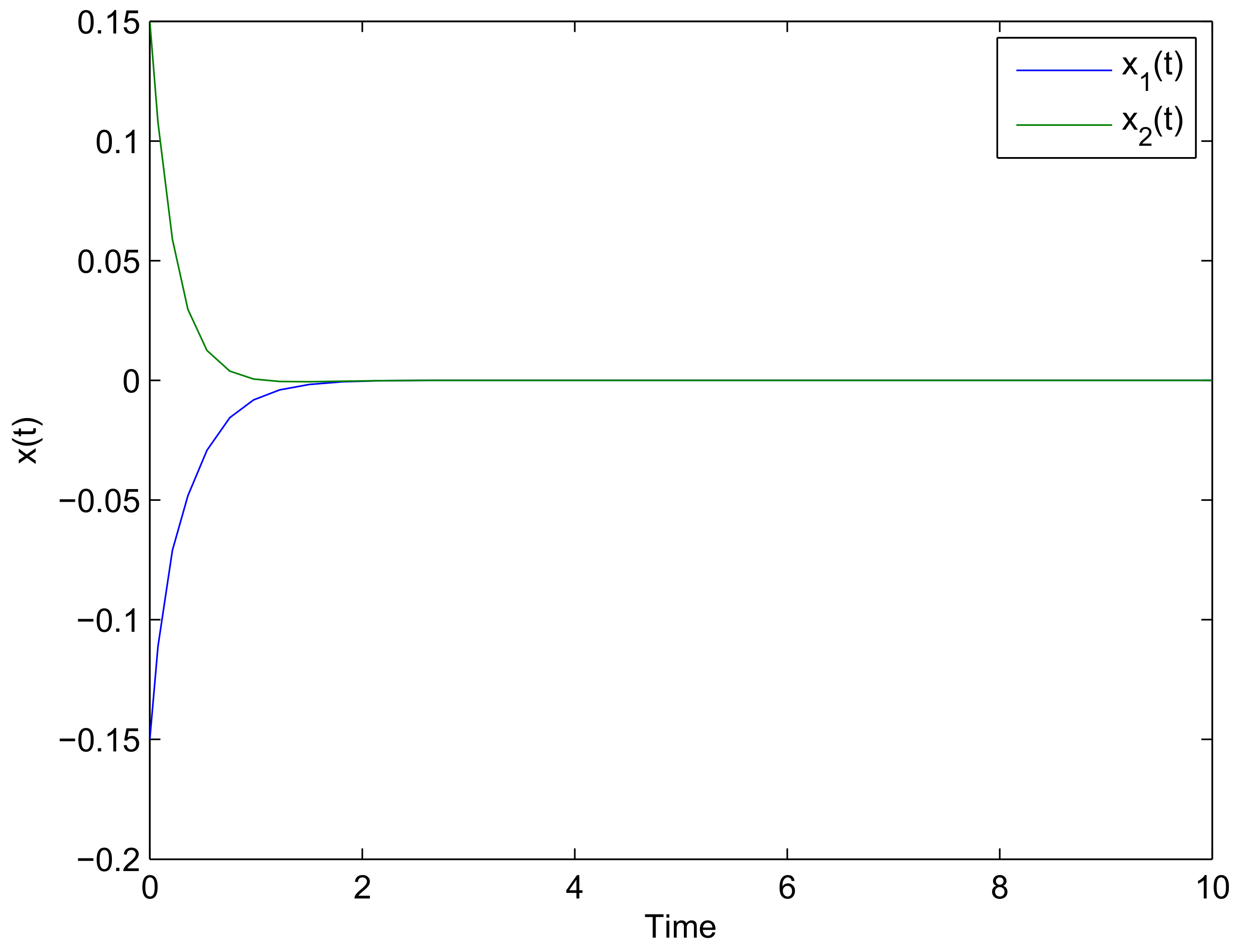
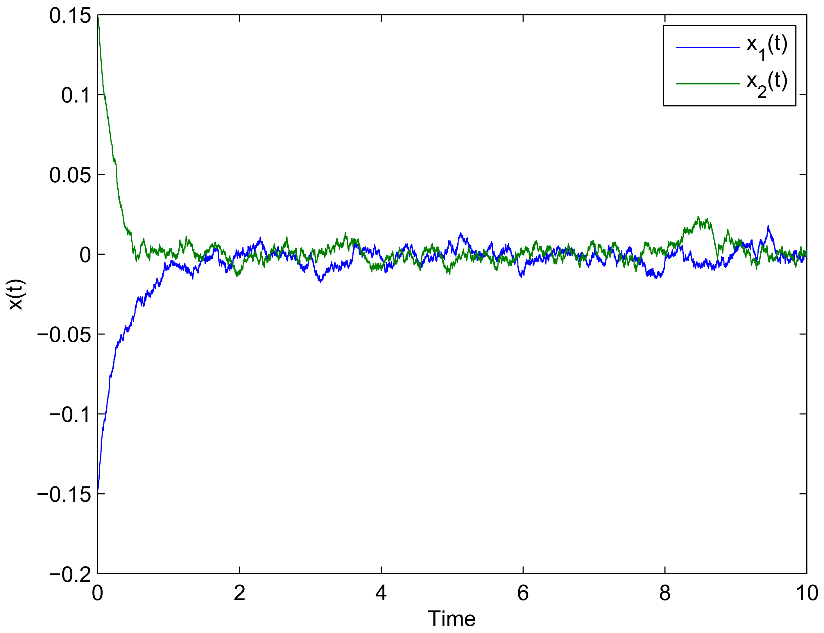
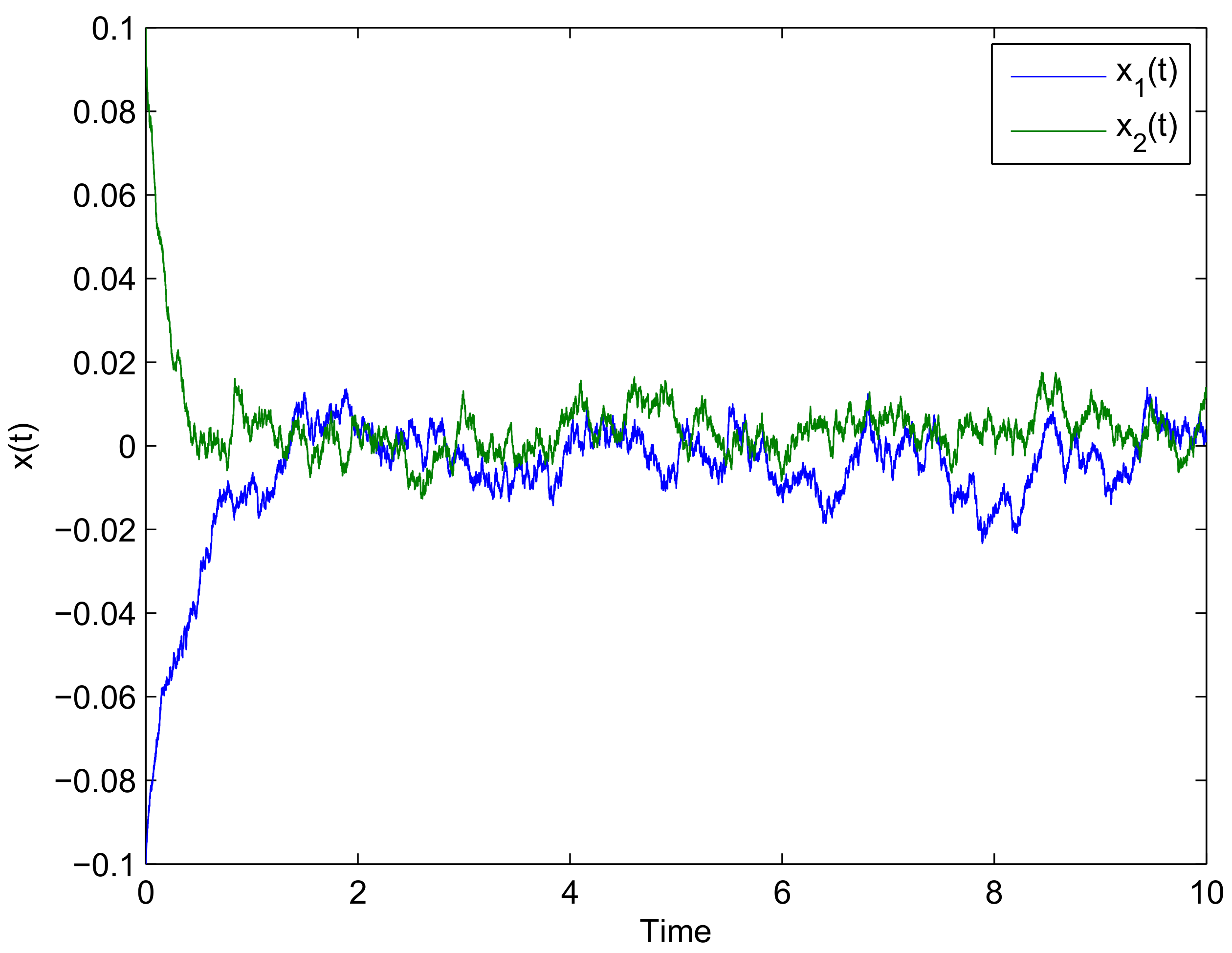
4. Numerical Examples

In this section, we provide two numerical examples with their simulations to demonstrate the effectiveness of our results.
Example 1.
Consider neural networks (3) with parameters as follows:
A = 4 0 0 4 , B = 0.7 0.2 0.4 0.1 , C = 0.7 0.8 0.5 0.9 , D = 0.7 0.7 0.1 0.4 , E = 0.1 0.2 0 0.4 , F = 0.5 0 0 0.3 , G = 0.5 0 0 0.4 , H = 0.4 0 0 0.2 , A 1 = 0.2 0.3 0 0.4 , B 1 = 0.4 0 0 0.4 , B 2 = 0.1 0 0 0.1 , B 3 = 0.1 0 0 0.1 , B 4 = 0.4 0 0.1 0.5 , C 1 = 0.2 0.1 0 0.5 , D 1 = 0.2 0.1 0 0.4 , E 1 = 0.1 0 0.1 0.3 , I = 1 0 0 1 , f ( · ) = g ( · ) = 0.2 | x 1 ( t ) + 1 | | x 1 ( t ) 1 | | x 2 ( t ) + 1 | | x 2 ( t ) 1 | , h ( · ) = tanh ( · ) .
From the conditions (14)–(17) of Theorem 1, we let α = 0.01 , h 1 = 0.1 , h 2 = 0.3 , d = 0.3 , d 1 = 0.5 , and τ = 0.4 . By using the LMI Toolbox in MATLAB, we obtain γ = 1.7637 ,
P 1 = 0.9248 0.1581 0.1581 0.7921 , P 2 = 0.0948 0.0501 0.0521 0.1187 , P 3 = 0.3225 0.0156 0.0156 0.3867 , P 4 = 0.0011 0.0006 0.0006 0.0013 , P 5 = 0.0020 0.0002 0.0001 0.0028 , P 6 = 0.0146 0.0020 0.0020 0.0161 , Q 1 = 0.5107 0.0462 0.0462 0.5004 , Q 2 = 0.4714 0.0328 0.0328 0.5166 , Q 3 = 0.4332 0.0043 0.0043 0.4422 , R 1 = 0.1392 0.0521 0.0521 0.1790 , R 2 = 0.4409 0.0481 0.0481 0.4248 , S 1 = 0.2493 0.0177 0.0177 0.2606 ,
S 2 = 0.8199 0.0161 0.0161 0.8399 , S 3 = 0.5445 0.0353 0.0353 0.6032 , U = 1.5450 0 0 1.5450 , U 2 = 1.0492 0 0 1.0492 , U 3 = 0.9085 0 0 0.9085 , W 1 = 10 3 7.4622 0.0421 0.0421 7.5146 , W 2 = 0.0518 0.0083 0.0083 0.0582 , W 3 = 0.0203 0.0007 0.0007 0.0207 , Z 1 = 0.0349 0.0002 0.0002 0.0353 , Z 2 = 0.8015 0.1874 0.1874 0.8118 , Z 3 = 0.2777 0.0028 0.0028 0.3139 .
The feedback control is given by
u ( t ) = B 1 P 1 1 x ( t ) = 0.4478 0.0894 0.0894 0.5228 x ( t ) , t 0 .
Moreover, the solution x ( t , ϕ ) of the system satisfies
| | x ( t , ϕ ) | | 1.2300 e 0.01 t | | ϕ | | c .
Figure 1 shows the response solution x ( t ) of the neural network system (3) where w ( t ) = 0 and the initial condition ϕ ( t ) = [ 0.1 0.1 ] T .
Figure 2 shows the response solution x ( t ) of the neural network system (3) with the initial condition ϕ ( t ) = [ 0.1 0.1 ] T .
Example 2.
Consider neural networks (39) with parameters as follows:
A = 5 0 0 4 , B = 0.7 0.2 0.4 0.1 , C = 0.7 0.8 0.5 0.9 , D = 0.7 0.7 1 0.4 , E = 0.1 0.2 0 0.4 , F = 0.5 0 0 0.3 , G = 0.5 0 0 0.4 , H = 0.4 0 0 0.2 , A 1 = 0.2 0.3 0 0.4 , B 1 = 0.3 0.1 0.2 0 , B 2 = 0.2 0 0 0.1 , B 3 = 0.1 0 0 0.3 , B 4 = 0.4 0 0.1 0.5 , C 1 = 0.2 0.1 0 0.5 , D 1 = 0.2 0.1 0 0.4 , E 1 = 0.1 0 0.1 0.3 , N = I = 1 0 0 1 , E A = E B = 0.4 0 0 0.4 , E C = 0.6 0 0 0.6 , E D = 0.2 0 0 0.2 , f ( · ) = g ( · ) = 0.2 | x 1 ( t ) + 1 | | x 1 ( t ) 1 | | x 2 ( t ) + 1 | | x 2 ( t ) 1 | , h ( · ) = tanh ( · ) , F ˜ ( t ) = sin ( t ) 0 0 sin ( t ) .
From the conditions (42)–(45) of Theorem 2, we let α = 0.01 , h 1 = 0.1 , h 2 = 0.3 , d = 0.3 , d 1 = 0.5 , and τ = 0.4 . By using the LMI Toolbox in MATLAB, we obtain
P 1 = 0.7130 0.0418 0.0418 0.6099 , P 2 = 0.0036 0.0030 0.0040 0.0074 , P 3 = 0.0842 0.0047 0.0047 0.0822 , P 4 = 10 4 3.9360 2.9290 4.1062 7.8329 , P 5 = 10 3 7.7772 0.7065 0.7274 7.8126 , P 6 = 0.0107 0.0088 0.0088 0.0175 , Q 1 = 0.3415 0.0824 0.0824 0.2748 , Q 2 = 0.0819 0.0527 0.0527 0.1249 , Q 3 = 0.1095 0.0935 0.0935 0.1220 , R 1 = 0.0417 0.0025 0.0025 0.0410 , R 2 = 0.6112 0.1130 0.1130 0.4407 , S 1 = 0.2316 0.0486 0.0486 0.0856 , S 2 = 0.2987 0.2759 0.2759 0.5621 , S 3 = 0.1103 0.0690 0.0690 0.1068 , U = 6.8799 0 0 6.8799 , U 2 = 0.3898 0 0 0.3898 , U 3 = 0.4546 0 0 0.4546 , W 1 = 10 3 0.0052 0.0047 0.0047 0.0084 , W 2 = 0.0016 0.0015 0.0015 0.0027 , W 3 = 0.0030 0.0029 0.0029 0.0053 ,
Z 1 = 0.0086 0.0079 0.0079 0.0140 , Z 2 = 0.4969 0.1357 0.1357 0.4097 , Z 3 = 0.0085 0.0078 0.0078 0.0137 .
The feedback control is given by
u ( t ) = B 1 P 1 1 x ( t ) = 0.4224 0.0290 0.0386 0.6584 x ( t ) , t 0 .
Moreover, the solution x ( t , ϕ ) of the system satisfies
| | x ( t , ϕ ) | | 1.2049 e 0.1 t | | ϕ | | c .
Figure 3 shows the response solution x ( t ) of the neural network system (39) where w ( t ) = 0 the initial condition ϕ ( t ) = [ 0.15 0.15 ] T .
Figure 4 shows the response solution x ( t ) of the neural network system (39) with the initial condition ϕ ( t ) = [ 0.15 0.15 ] T .
Remark 5.
The advantages of Examples 1 and 2 are the lower bound of the delay h 1 0 and interval time-varying delay and distributed time-varying delay are non-differentiable. Moreover, in these examples we still investigate various activation functions and mixed time-varying delays in state and feedback control. Thus, the neural network conditions derived in [23] cannot be applied to these examples.

5. Conclusions

In this paper, the problem of a robust H control for a class of uncertain systems with interval and distributed time-varying delays was investigated. It is assumed that the interval and distributed time-varying delays are not necessary to be differentiable. Firstly, we considered an H control for exponential stability of neural network with interval and distributed time-varying delays via hybrid feedback control and a robust H control for exponential stability of uncertain neural network with interval and distributed time-varying delays via hybrid feedback control. Secondly, by using a novel Lyapunov–Karsovskii functional that the Lyapunov matrix P i ( i = 1 , 2 , , 6 ) do not need to be positive definiteness, the employment of a tighter bounding technique, some slack matrices and newly introduced convex combination condition in the calculation, improved delay-dependent sufficient conditions for the robust H control with exponential stability of the system are obtained. Finally, numerical examples have been given to illustrate the effectiveness of the proposed method. The results in this paper improve the corresponding results of the recent works. In the future work, the derived results and methods in this work are expected to be applied to other systems, for example, H state estimation of neural networks, exponential passivity of neural networks, neutral-type neural networks, stochastic neural networks, T-S fuzzy neural networks, and so on [24,38,39,40,41].

Author Contributions

Conceptualization, T.B. and W.W; Data curation, R.S. and S.N.; Formal analysis, C.C. and T.B.; Funding acquisition, W.W.; Investigation, R.S. and S.N.; Methodology, C.C., T.B., W.W. and S.N.; Resources, R.S.; Software, C.C.; Supervision, T.B. and W.W. All authors have read and agreed to the published version of the manuscript.

Funding

The first author was financially supported by the Science Achievement Scholarship of Thailand (SAST). The second author was financially supported by Khon Kaen University. The fourth author was supported by the Unit of Excellence in Mathematical Biosciences (FF64-UoE042) supported by the University of Phayao.

Institutional Review Board Statement

Not applicable.

Informed Consent Statement

Not applicable.

Data Availability Statement

The data presented in this study are available on request from the corresponding author.

Acknowledgments

The authors thank the reviewers for their valuable comments and suggestions, which led to the improvement of the content of the paper.

Conflicts of Interest

The authors declare no conflict of interest.

References

  1. Cheng, X.M.; Gui, W.H.; Gan, Z.J. Robust reliable control for a class of time-varying uncertain impulsive systems. J. Cent. South Univ. Technol. 2005, 12, 199–202. [Google Scholar] [CrossRef]
  2. Gao, J.; Huang, B.; Wang, Z.; Fisher, D.G. Robust reliable control for a class of uncertain nonlinear systems with time-varying multi-state time delays. Int. J. Syst. Sci. 2001, 32, 817–824. [Google Scholar] [CrossRef]
  3. Veillette, R.J.; Medanic, J.V.; Perkins, W.R. Design of reliable control systems. IEEE Trans. Autom. Control 1992, 37, 290–304. [Google Scholar] [CrossRef]
  4. Wang, Z.; Huang, B.; Unbehauen, H. Robust reliable control for a class of uncertain nonlinear state-delayed systems. Automatica 1999, 35, 955–963. [Google Scholar] [CrossRef]
  5. Alwan, M.S.; Liu, X.Z.; Xie, W.C. On design of robust reliable H control and input–to-state stabilization of uncertain stochastic systems with state delay. Commun. Nonlinear Sci. Numer. Simulat. 2013, 18, 1047–1056. [Google Scholar] [CrossRef]
  6. Yue, D.; Lam, J.; Ho, D.W.C. Reliable H control of uncertain descriptor systems with multiple delays. IEE Proc. Control Theory Appl. 2003, 150, 557–564. [Google Scholar] [CrossRef]
  7. Xiang, Z.G.; Chen, Q.W. Robust reliable control for uncertain switched nonlinear systems with time delay under asynchronous switching. Appl. Math. Comput. 2010, 216, 800–811. [Google Scholar] [CrossRef]
  8. Wang, Z.D.; Wei, G.L.; Feng, G. Reliable H control for discrete-time piecewise linear systems with infinite distributed delays. Automatica 2009, 45, 2991–2994. [Google Scholar] [CrossRef] [Green Version]
  9. Mahmoud, M.S. Reliable decentralized control of interconnected discrete delay systems. Automatica 2012, 48, 986–990. [Google Scholar] [CrossRef]
  10. Suebcharoen, T.; Rojsiraphisal, T.; Mouktonglang, T. Controlled current quality improvement by multi-target linear quadratic regulator for the grid integrated renewable energy system. J. Anal. Appl. 2021, 19, 47–66. [Google Scholar]
  11. Faybusovich, L.; Mouktonglang, T.; Tsuchiya, T. Implementation of infinite-dimensional interior-point method for solving multi-criteria linear-quadratic control problem. Optim. Methods Softw. 2006, 21, 315–341. [Google Scholar] [CrossRef]
  12. Haykin, S. Neural Networks; Prentice-Hall: Englewood Cliffs, NJ, USA, 1994. [Google Scholar]
  13. Yang, X.; Song, Q.; Liang, J.; He, B. Finite-time synchronization of coupled discontinuous neural networks with mixed delays and nonidentical perturbations. J. Franklin Inst. 2015, 352, 4382–4406. [Google Scholar] [CrossRef]
  14. Zhang, H.; Wang, Z. New delay-dependent criterion for the stability of recurrent neural networks with time-varying delay. Sci. China Inf. Sci. 2009, 52, 942–948. [Google Scholar] [CrossRef]
  15. Li, X.; Souza, C.E.D. Delay-dependent robust stability and stabilization of uncertain linear delay systems: A linear matrix inequality approach. IEEE Trans. Automat. Control 1997, 42, 1144–1148. [Google Scholar] [CrossRef]
  16. Ali, M.S.; Balasubramaniam, P. Exponential stability of time delay systems with nonlinear uncertainties. Int. J. Comput. Math. 2010, 87, 1363–1373. [Google Scholar] [CrossRef]
  17. Ali, M.S. On exponential stability of neutral delay differential system with nonlinear uncertainties. Commun. Nonlinear Sci. Numer. Simul. 2012, 17, 2595–2601. [Google Scholar]
  18. Yoneyama, J. Robust H control of uncertain fuzzy systems under time-varying sampling. Fuzzy Sets Syst. 2010, 161, 859–871. [Google Scholar] [CrossRef]
  19. Yoneyama, J. Robust H filtering for sampled-data fuzzy systems. Fuzzy Sets Syst. 2013, 217, 110–129. [Google Scholar] [CrossRef]
  20. Francis, B.A. A Course in H Control Theory; Springer: Berlin, Germany, 1987. [Google Scholar]
  21. Keulen, B.V. H Control For Distributed Parameter Systems: A State-Space Approach; Birkhauser: Boston, MA, USA, 1993. [Google Scholar]
  22. Petersen, I.R.; Ugrinovskii, V.A.; Savkin, A.V. Robust Control Design Using H Methods; Springer: London, UK, 2000. [Google Scholar]
  23. Du, Y.; Liu, X.; Zhong, S. Robust reliable H control for neural networks with mixed time delays. Chaos Solitons Fractals 2016, 91, 1–8. [Google Scholar] [CrossRef]
  24. Lakshmanan, S.; Mathiyalagan, K.; Park, J.H.; Sakthivel, R.; Rihan, F.A. Delay-dependent H state estimation of neural networks with mixed time-varying delays. Neurocomputing 2014, 129, 392–400. [Google Scholar] [CrossRef]
  25. Tian, E.; Yue, D.; Zhang, Y. On improved delay-dependent robust H control for systems with interval time-varying delay. J. Franklin Inst. 2011, 348, 555–567. [Google Scholar] [CrossRef]
  26. Duan, Q.; Su, H.; Wu, Z.G. H state estimation of static neural networks with time-varying delay. Neurocomputing 2012, 97, 16–21. [Google Scholar] [CrossRef]
  27. Liu, Y.; Lee, S.; Kwon, O.; Park, J. A study on H state estimation of static neural networks with time-varying delays. Appl. Math. Comput. 2014, 226, 589–597. [Google Scholar] [CrossRef]
  28. Ali, M.S.; Saravanakumar, R.; Arik, S. Novel H state estimation of static neural networks with interval time-varying delays via augmented Lyapunov–Krasovskii functional. Neurocomputing 2016, 171, 949–954. [Google Scholar]
  29. Thanh, N.T.; Phat, V.N. H control for nonlinear systems with interval non-differentiable time-varying delay. Eur. J. Control 2013, 19, 190–198. [Google Scholar] [CrossRef]
  30. Gu, K.; Kharitonov, V.L.; Chen, J. Stability of Time-Delay Systems; Birkhäuser: Berlin, Germany, 2003. [Google Scholar]
  31. Sun, J.; Liu, G.P.; Chen, J. Delay-dependent stability and stabilization of neutral time-delay systems. Internat. J. Robust Nonlinear Control 2009, 19, 1364–1375. [Google Scholar] [CrossRef]
  32. Wang, Z.; Liu, Y.; Fraser, K.; Liu, X. Stochastic stability of uncertain Hopfield neural networks with discrete and distributed delays. Phys. Lett. A 2006, 354, 288–297. [Google Scholar] [CrossRef] [Green Version]
  33. Qian, W.; Cong, S.; Sun, Y.; Fei, S. Novel robust stability criteria for uncertain systems with time-varying delay. Appl. Math. Comput. 2009, 215, 866–872. [Google Scholar] [CrossRef]
  34. Xu, S.; Lam, J.; Zou, Y. New results on delay-dependent robust H control for systems with time-varying delay. Automatica 2006, 42, 343–348. [Google Scholar] [CrossRef]
  35. Peng, C.; Tian, Y.C. Delay-dependent robust H control for uncertain systems with time-varying delay. Inf. Sci. 2009, 179, 3187–3197. [Google Scholar] [CrossRef] [Green Version]
  36. Yan, H.C.; Zhang, H.; Meng, M.Q. Delay-range-dependent robust H control for uncertain systems with interval time-varying delays. Neurocomputing 2010, 73, 1235–1243. [Google Scholar] [CrossRef]
  37. Wang, C.; Shen, Y. Improved delay-dependent robust stability criteria for uncertain time delay systems. Appl. Math. Comput. 2011, 218, 2880–2888. [Google Scholar] [CrossRef]
  38. Wu, Z.G.; Park, J.H.; Su, H.; Chu, J. New results on exponential passivity of neural networks with time-varying delays. Nonlinear Anal. Real World Appl. 2012, 13, 1593–1599. [Google Scholar] [CrossRef]
  39. Manivannan, R.; Samidurai, R.; Cao, J.; Alsaedi, A.; Alsaadi, F.E. Delay-dependent stability criteria for neutral-type neural networks with interval time-varying delay signals under the effects of leakage delay. Adv. Differ. Equ. 2018, 2018, 1–25. [Google Scholar] [CrossRef]
  40. Saravanakumar, R.; Mukaidani, H.; Muthukumar, P. Extended dissipative state estimation of delayed stochastic neural networks. Neurocomputing 2020, 406, 244–252. [Google Scholar] [CrossRef]
  41. Shanmugam, S.; Muhammed, S.A.; Lee, G.M. Finite-time extended dissipativity of delayed Takagi-Sugeno fuzzy neural networks using a free-matrixbased double integral inequality. Neural Comput. Appl. 2019, 32, 8517–8528. [Google Scholar]
Figure 1. Response solution of the system (3) where w ( t ) = 0 .
Computation 09 00062 g001
Figure 2. Response solution of the system (3).
Computation 09 00062 g002
Figure 3. Response solution of the system (39) where w ( t ) = 0 .
Computation 09 00062 g003
Figure 4. Response solution of the system (39).
Computation 09 00062 g004
Publisher’s Note: MDPI stays neutral with regard to jurisdictional claims in published maps and institutional affiliations.

