Article

Computational Performance of Disparate Lattice Boltzmann Scenarios under Unsteady Thermal Convection Flow and Heat Transfer Simulation

1
Resources Production and Safety Engineering (REPS) Laboratory, Department of Earth Resources Engineering, Kyushu University, Fukuoka 812-0395, Japan
2
Institute for Future Engineering (IFENG), 2-6-11 Fukagawa Koto-ku, Tokyo 135-8473, Japan
*
Author to whom correspondence should be addressed.
Submission received: 5 April 2021 / Revised: 19 May 2021 / Accepted: 27 May 2021 / Published: 31 May 2021
(This article belongs to the Section Computational Engineering)

Abstract

:
The present work highlights the capacity of disparate lattice Boltzmann strategies in simulating natural convection and heat transfer phenomena during the unsteady period of the flow. Within the framework of Bhatnagar-Gross-Krook collision operator, diverse lattice Boltzmann schemes emerged from two different embodiments of discrete Boltzmann expression and three distinct forcing models. Subsequently, computational performance of disparate lattice Boltzmann strategies was tested upon two different thermo-hydrodynamics configurations, namely the natural convection in a differentially-heated cavity and the Rayleigh-Bènard convection. For the purposes of exhibition and validation, the steady-state conditions of both physical systems were compared with the established numerical results from the classical computational techniques. Excellent agreements were observed for both thermo-hydrodynamics cases. Numerical results of both physical systems demonstrate the existence of considerable discrepancy in the computational characteristics of different lattice Boltzmann strategies during the unsteady period of the simulation. The corresponding disparity diminished gradually as the simulation proceeded towards a steady-state condition, where the computational profiles became almost equivalent. Variation in the discrete lattice Boltzmann expressions was identified as the primary factor that engenders the prevailed heterogeneity in the computational behaviour. Meanwhile, the contribution of distinct forcing models to the emergence of such diversity was found to be inconsequential. The findings of the present study contribute to the ventures to alleviate contemporary issues regarding proper selection of lattice Boltzmann schemes in modelling fluid flow and heat transfer phenomena.

1. Introduction

The Lattice Boltzmann Method (LBM) has raised considerable interest amongst the community of computational fluid dynamics (CFD) due to its efficacy in handling multitude fluid flow problems. Relying on the statistical mechanics, LBM regards the flowing materials through the collective behaviour of the accompanying molecules [1,2]. It differs from traditional CFD methods in sense that it solves the representative Boltzmann expression of the flowing substances rather than directly handling the corresponding hydrodynamics equations in their operations. Because of this unique feature, modelling a flow problem using LBM has several advantages, including a clear algorithm [3], straightforward treatment of boundary conditions [4], and innate feasibility for parallel computing architecture [5]. As a promising numerical tool, LBM is currently a vibrant research topic in the discipline of CFD.
As far as modelling the flow problem using LBM is concerned, two properties are routinely considered: (a) the discrete lattice Boltzmann expressions, and (b) the discrete forcing schemes. The former parameter has been extensively discussed in the literature. Ubertini et al. [6] investigated three distinct models of discrete lattice Boltzmann expression for hydrodynamics simulation, namely the first-order, the second-order, and the scheme derived through implementation of the Verlet discretisation, which all showed a second-order accuracy both in spatial and time coordinates with respect to the convective system. They argued that such equivalence breaks down when the nature of the physical systems necessitates the inclusion of external forcing expression.
Silva and Semiao [7] carried out a comprehensive assessment of distinct lattice Boltzmann remarks using Chapman-Enskog analysis. Guo et al. [8] highlight the significance of the different lattice Boltzmann schemes towards the accuracy of the recovered Navier-Stokes expression from the Chapman-Enskog analysis. Additionally, they mentioned that the choice of discrete forcing model depends heavily upon the exactitude of the restored continuum hydrodynamics representation.
On the other hand, the discrete forcing model in LBM is the other prominent property when modelling the flow is sought. Several authors have proposed diverse expressions to accommodate external forcing term in the generic lattice Boltzmann equation. Luo [9] was among the first authors to propose a mathematical expression for the discrete forcing term in LBM, alongside with He et al. [10] and Guo et al. [8,11]. Later on, Kupershtokh et al. [12] introduced a forcing model based on the association of exact-difference-method upon the corresponding Boltzmann equation.
The presence of different mathematical expressions for both the discrete lattice Boltzmann equation and the forcing model offers diverse LBM strategies for hydrodynamics modelling. However, choosing a suitable approach is still a matter of debate. To alleviate such issues, Mohamad and Kuzmin [13] investigated the behaviour of three different forcing models by simulating natural convection in closed and open-ended cavities. They found that the investigated forcing models produced equivalent numerical solutions at steady-state conditions.
Subsequently, Krivovichev [14] presented a comprehensive evaluation regarding stability analysis of the six widely-used forcing models based on the application of the von Neumann method to linear approximation of the system of nonlinear lattice Boltzmann expressions. They found that better stability properties prevailed upon the forcing models that are implicit in their nature. Zheng et al. [15] found that as long as the simulation comprises low Mach number flow, different forcing schemes in LBM would return equivalent steady-state solutions.
It is apparent from the available literature that few works have looked into the implications of both distinct lattice Boltzmann expressions and different forcing models in LBM simulation. Moreover, the primary focus of the published works has revolved around the discrepancy in the computational characteristics of distinct LBM scenarios during the steady-state condition of the simulation, leaving the behaviour during the unsteady period of the flow unexplained. Therefore, the present work aims to expand the evaluation of the capacity of disparate LBM schemes by incorporating the variety in both the discrete lattice Boltzmann expressions and the discrete forcing models into the workflow of the assessment. Emphasis was given upon revealing the computational characteristic of distinct LBM scenarios during the unsteady-period of the simulation. The steady-state solutions were considered for the exhibition and validation purposes.
In this study, two different embodiments of discrete Boltzmann expression and three distinct forcing models were incorporated into the analysis. For the sake of providing comprehensive evaluation, the capacity of disparate LBM schemes was tested upon simulating two non-isothermal thermo-hydrodynamics systems, namely natural convection in a differentially-heated cavity and Rayleigh-Bènard convection.
The current research article is organized as follows. Section 2 presents the foundational aspect of natural convection and heat transfer arrangement. Section 3 describes the distinct LBM strategies for simulating the concomitant physical phenomena. Section 4 deals with theoretical outlook of disparate LBM scenarios, while the results of numerical testing are discussed in Section 5. Some concluding remarks are posed in Section 6.

2. Governing Mathematical Remarks and Principal Dimensionless Groups

Natural convection phenomena is governed by two flowing materials that propagate simultaneously and synergistically within the flow domain, namely the fluid and thermal substances. Accordingly, the natural convection is governed by three fundamental equations, namely, the continuity, Navier-Stokes, and heat equations [16], expressed as
ρ t + x α ( ρ u α ) = 0
t ( ρ u α ) + x β ( ρ u α u β ) = p x β + μ x β ( u α x β + u β x α ) + F α
T t + x α ( T u α ) = x α ( D T x α ) ,
where ρ , u i , p , T , μ and D denote the fluid density, velocity, pressure, temperature, dynamic viscosity, and thermal diffusion coefficient, respectively. The contribution from the buoyancy effect was designated by F α .
In the present work, the natural convection was examined under the Boussinesq approximation [13,17]. As such, it neglected the contributions to the dynamical behaviour of the flowing substances from viscous heat dissipation and compression caused. Therefore, the buoyancy term occupies the following definition [13]:
F α = ρ G α β T ( T T ref ) ,
where G α specifies the gravitational acceleration, β T depicts the thermal expansion coefficient, and T ref represents the assigned reference temperature.
It is customary within CFD to express the associated physical quantities using non-dimensional units. For natural convection phenomena, the key dimensionless groups were identified as follows:
N u = h L ρ D c p ; P r = υ D ; R a = G y β T ( T hot T cold ) L 3 υ D ,
where Nu , Pr , and Ra designate the Nusselt, Prandtl, and Rayleigh number, accordingly. T hot and T cold denote the hot and cold temperature conditions, respectively. Physical quantities of h , c p , and L represent, respectively, the heat transfer coefficient, fluid specific heat capacity, and the characteristic length of the domain.
Furthermore, the present work uses the following generic dimensionless expressions to designate the horizontal and vertical length of the flow domain.
x * = x L ; y * = y L ; u α * = u α L D .
In Equation (6), x and y express, respectively, the horizontal and vertical length of the investigated domain.

3. Lattice Boltzmann Expressions from Distinct Truncation Order

In the present work, consideration was given to the double-distribution-function (DDF) approach to establish a proper representation of the dynamical entities [17]. This would mean that the prevalence of two continuous Boltzmann expressions, which should be discretised either by capturing only the first-truncation order or considering up to the second-truncation term of the expanded-Boltzmann equation. Regardless the approach considered, different representations of the discrete lattice Boltzmann equation are obtained.
For the fluid component, the first- and second-order discrete lattice Bhatnagar-Gross-Krook (BGK) equations are expressed as follows:
f i ( x α + ξ i α Δ t , t + Δ t ) f i ( x α , t ) = Δ t τ υ ( f i ( x α , t ) f i e q ( x α , t ) ) + R i ( x α , t ) Δ t
f ¯ i ( x α + ξ i α Δ t , t + Δ t ) f ¯ i ( x α , t ) = Δ t τ ¯ υ ( f ¯ i ( x α , t ) f i e q ( x α , t ) ) + R i ( x α , t ) Δ t ( 1 Δ t 2 τ ¯ υ ) ,
where f i indicates the discrete fluid populations, ξ i α specifies the discrete velocity of fluid particles, R i designates the discrete form of the external force term, τ υ denotes the relaxation time for fluid particles, and Δ t specifies the discrete time step.
For the second-order lattice BGK model, the corresponding discrete fluid population f ¯ i and its corresponding relaxation time τ ¯ υ were defined accordingly as in [6,10]:
f ¯ i = f i + Δ t 2 τ υ ( f i f i e q ) R i Δ t 2
τ ¯ υ = τ υ + Δ t 2 ,
where f i e q depicts the equilibrium condition of the fluid population.
The equilibrium distribution function f i e q occupies the following remark:
f i e q = ρ w i ( 1 + ξ i α u α c s 2 + ( ξ i α u α ) 2 2 c s 4 u α u β 2 c s 2 ) ,
where c s designates the lattice speed of sound and w i represents the discrete weighting coefficient.
In the present work, the D2Q9 velocity arrangement was selected to model fluid displacements. Such configuration satisfies the following descriptions:
ξ i α = { ( 0 , 0 ) , for   i = 0 ( 1 , 0 ) , ( 0 , 1 ) , ( 1 , 0 ) , ( 0 , 1 ) , for   i = 1 , 2 , 3 , 4 ( 1 , 1 ) , ( 1 , 1 ) , ( 1 , 1 ) , ( 1 , 1 ) , for   i = 5 , 6 , 7 , 8
w i = { 4 9 , for   i = 0 1 9 , for   i = 1 , 2 , 3 , 4 1 36 , for   i = 5 , 6 , 7 , 8 .
Apart from the dichotomy in the lattice BGK representation for fluid movements, the discrete manifestation of forcing term R i also occupies diverse expressions. In this study, three of the most prominent R i models were selected for the evaluation, namely the scheme proposed by Luo [9], Guo et al. [8], and Kupershtokh et al. [12], expressed respectively as follows:
R i = w i ξ i α F α c s 2
R i = w i ( ξ i α u α c s 2 + ( ξ i α u α ) ξ i α c s 4 ) F α
R i = f i e q ( ρ , u α + Δ u α ) f i e q ( ρ , u α ) .
For the thermal constituent, due to the absence of external force term, the discretisation operation of Boltzmann representation of thermal substance is not affected by the selected truncation order. Therefore, the lattice BGK formula representing the thermal dissemination only occupies a single mathematical expression, namely,
g i ( x α + e i α Δ t , t + Δ t ) g i ( x α , t ) = Δ t τ D ( g i ( x α , t ) g i e q ( x α , t ) ) ,
where g i identifies the discrete thermal population, e i α denotes the discrete velocity of thermal particles, and τ D designates the relaxation time for thermal elements.
The associated thermal equilibrium population g i e q was defined as follows:
g i e q = z i T ( 1 + e i α u α c s 2 + ( e i α u α ) 2 2 c s 4 u α u β 2 c s 2 ) .
For thermal dissemination, D2Q5 discrete velocity set was adopted. Implementation of fewer velocity directions to represent thermal displacements was possible due to the lower isotropy nature pertinent to thermal populations in the corresponding lattice Boltzmann arrangement. As can be seen in Appendix B, the associated Chapman-Enskog analysis of thermal particles only necessitates low-order moment expansion terms in order to recover correct macroscopic heat formulation. Consequently, the isotropy requirement for thermal displacement modelling in LBM can be conducted properly by fewer lattice arrangement, such as the D2Q5 velocity set [2].
For the adopted D2Q5 configuration, the discrete velocity of thermal particles e i α and their corresponding weighting factor z i adhere to the following descriptions:
e i α = { ( 0 , 0 ) , for   i = 0 ( 1 , 0 ) , ( 0 , 1 ) , ( 1 , 0 ) , ( 0 , 1 ) , for   i = 1 , 2 , 3 , 4
z i = { 2 6 , for   i = 0 1 6 , for   i = 1 , 2 , 3 , 4 .
At this point, it is apparent that there exist distinct strategies to administer natural convection and heat transfer modelling with LBM.
Table 1 outlines the plausible LBM scenarios considered in the present work, as well as the corresponding scheme.

4. Recovery of the Macroscopic Thermo-Hydrodynamics Expressions from Disparate LBM Arrangements in Natural Convection Heat Transfer Modelling

As a thermo-hydrodynamics solver, LBM is closely tied to the macroscopic heat and mass transport formulations. It is therefore pivotal to uncover the capacity of each considered LBM schemes in returning the fundamental macroscopic relationships. This objective was fulfilled through evaluating the Chapman-Enskog analysis [7,8,18]. Appendix A and Appendix B provide the details of undertaken procedures for the associated fluid and thermal components, respectively.
From the corresponding Chapman-Enskog analysis, the restored macroscopic equations of mass, momentum, and heat transport were captured as follows:
ρ t + x α ( ρ u α ) = x α ( F α ( m Δ t m ( Δ t ) 2 2 σ Δ t 2 φ ) )
t ( ρ u α ) + x β ( ρ u α u β ) = x β ( ρ c s 2 δ α β ) + ρ c s 2 ( σ Δ t 2 ) x β ( u α x β + u β x α ) + ( φ + m Δ t σ ) F α + t ( F α ( m Δ t m ( Δ t ) 2 2 σ Δ t 2 φ ) ) + ( σ Δ t 2 ) ( φ + m Δ t σ ) x β ( u α F β + F α u β ) ( σ Δ t 2 ) x β x γ ( ρ u α u β u γ ) σ φ x β i ξ i α ξ i β R i .
T t + x α ( T u α ) = x α ( c s 2 ( τ D Δ t 2 ) T x α ) + ( τ D Δ t 2 ) x α ( T ( u α t + x β ( u α u β ) ) ) .
In Equation (22), the term i ξ i α ξ i β R i specifies the second-order moment of the forcing term. Details regarding the mathematical expressions of all the associated forcing moments are appended in Appendix A of this manuscript. In Equations (21) and (22), quantities m , σ , and φ occupy the following definitions:
m = { 0 , for   scenario   IA ,   IB   and   IC 1 2 , for   scenario   IIA ,   IIB   and   IIC
σ = { τ υ , for   scenario   IA ,   IB   and   IC τ ¯ υ , for   scenario   IIA ,   IIB   and   IIC
φ = { 1 , for   scenario   IA ,   IB   and   IC ( 1 Δ t 2 τ ¯ υ ) , for   scenario   IIA ,   IIB   and   IIC .
From the recovered thermo-hydrodynamics expressions of Equations (21)–(23), it was observed that each of the corresponding LBM scenarios returns the macroscopic hydrodynamics relationships with residual fractions. Such properties occupy different mathematical expressions depending upon the selected LBM scenarios. Table 2 summarizes the corresponding mathematical remarks of hydrodynamics residual fractions from distinct LBM schemes. On the other hand, the restored heat formulation of Equation (23) contains only one residual fraction, appropriately depicted by the last term on the right hand side of the formula. Nevertheless, it is important to mention that the particular thermal residual fraction incorporates momentum terms from the fluid constituents within its expression.
Consequently, the residual term in the recovered heat equation is linked indirectly to the residual terms in the restored Navier-Stokes formula of Equation (22).

5. Numerical Results and Discussions

To test the computational performance of disparate LBM scenarios, two distinctive thermo-hydrodynamics flow systems (the natural convection in a differentially-heated cavity and the Rayleigh-Bènard convection) were selected. The simulations of both physical phenomena were performed in a two-dimensional close system under the condition of Ra = 10 4 and Pr = 0 . 71 . The computational workloads were administered upon the graphical processing unit (GPU) ecosystem so as to expedite the analyses. In such physical arrangements, the Mach number (Ma) was defined as
M a = u char c s = R a υ 2 P r H 2 c s 2 ,
where u char designates the characteristic velocity of the flowing material.
The particular property was defined as
u char = G y β T ( Θ hot Θ cold ) H = R a υ 2 P r H 2 ,
where Θ hot and Θ cold specify, respectively, the dimensionless hot and cold temperatures. In general, the dimensionless temperature is expressed as
Θ = T T ref T hot T cold ,
where T ref denotes the reference temperature.
The expressions for fluid kinematic viscosity υ and thermal diffusivity D were obtained, respectively, as
υ = { c s 2 ( τ υ Δ t 2 ) , for   scenario   IA ,   IB   and   IC c s 2 ( τ ¯ υ Δ t 2 ) , for   scenario   IIA ,   IIB   and   IIC
D = c s 2 ( τ D Δ t 2 ) .

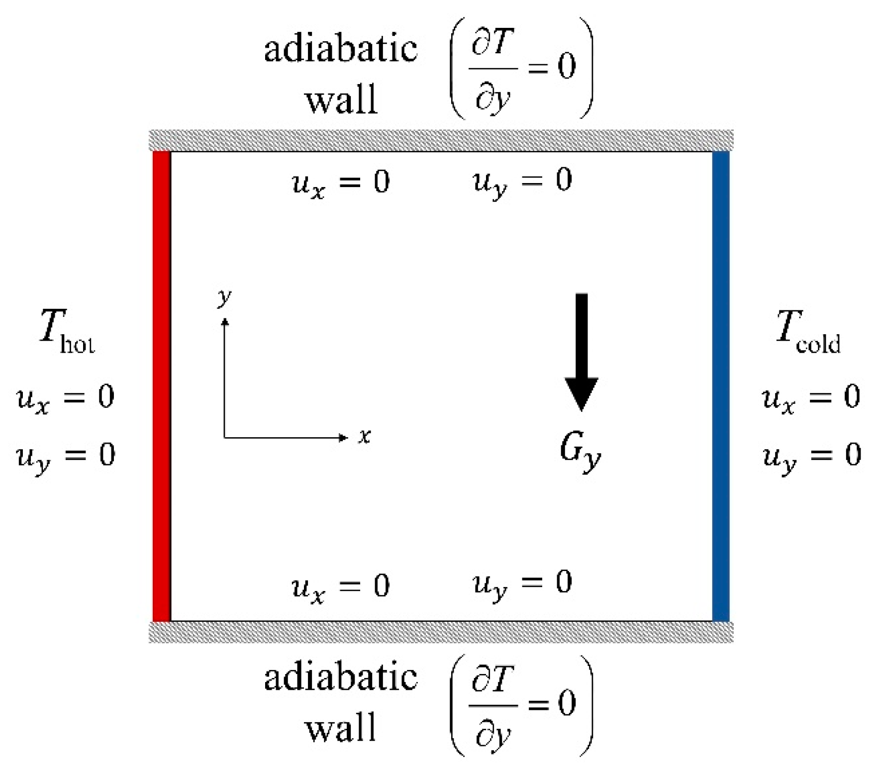
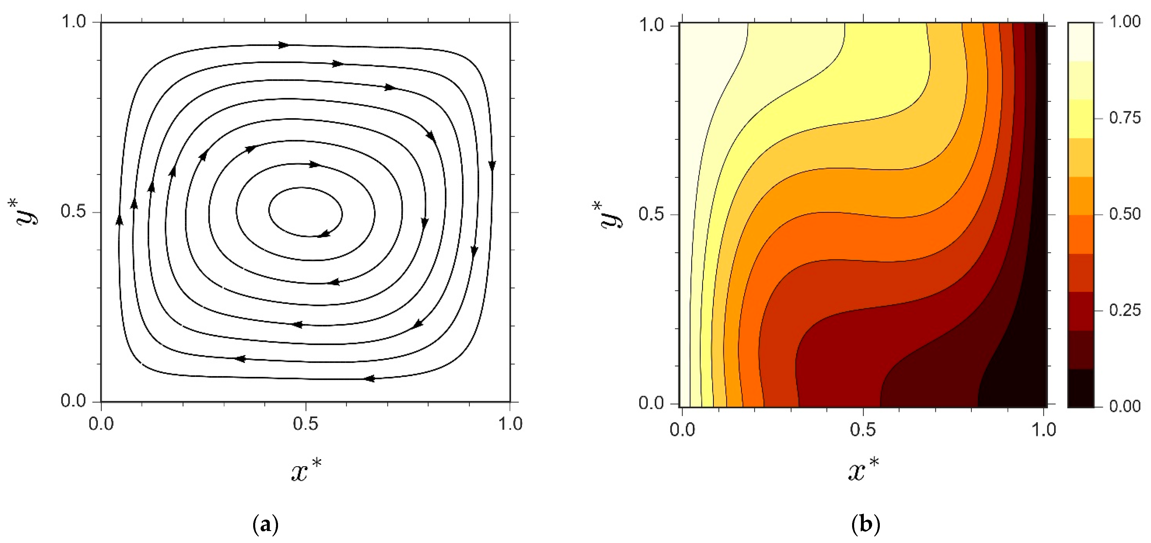
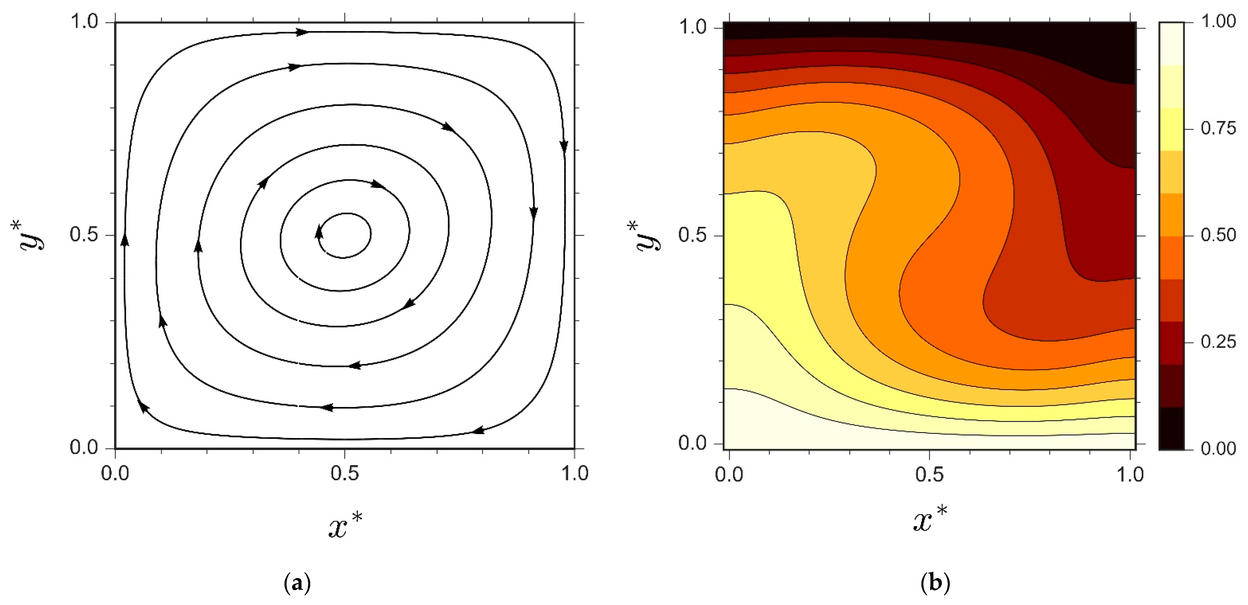
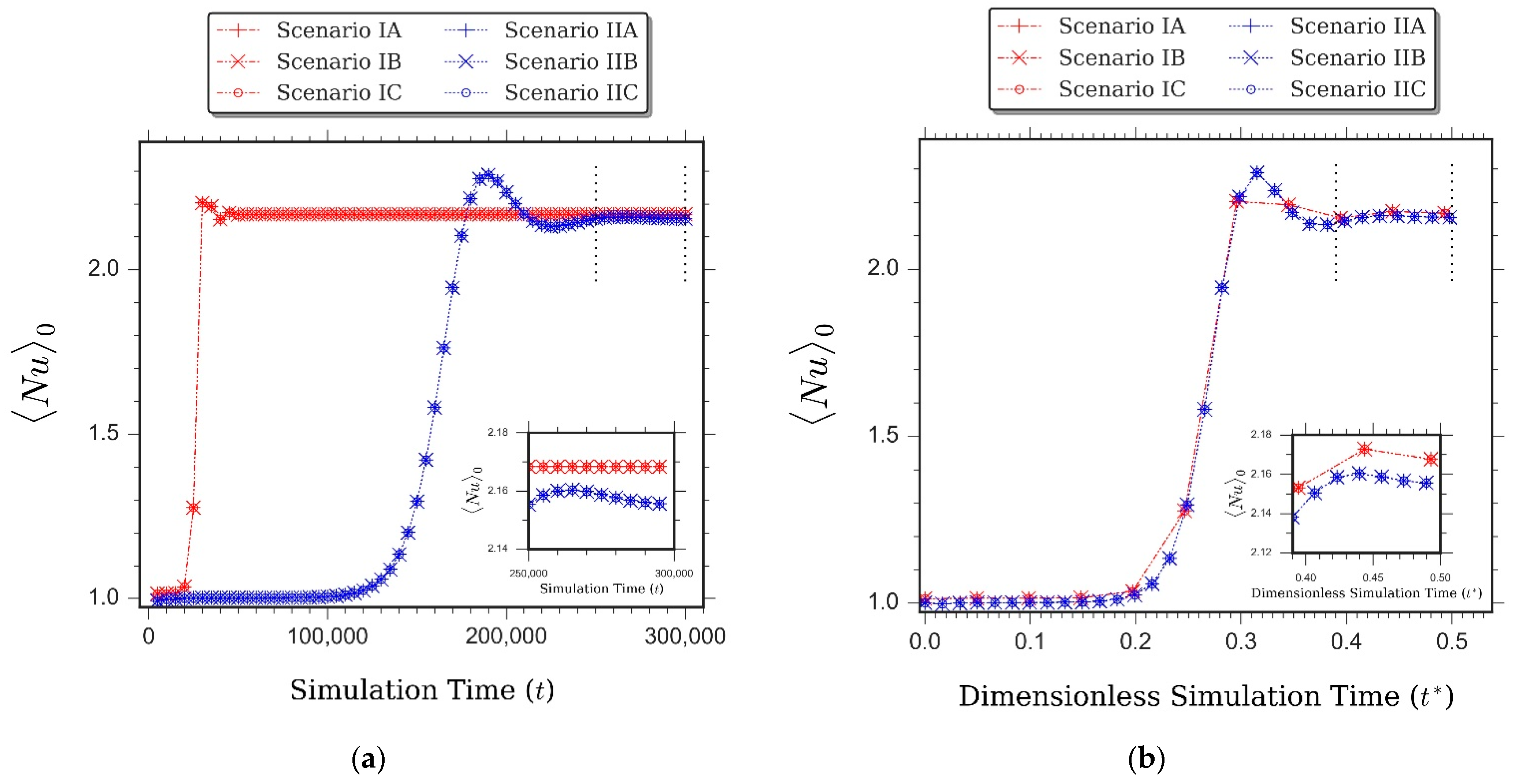
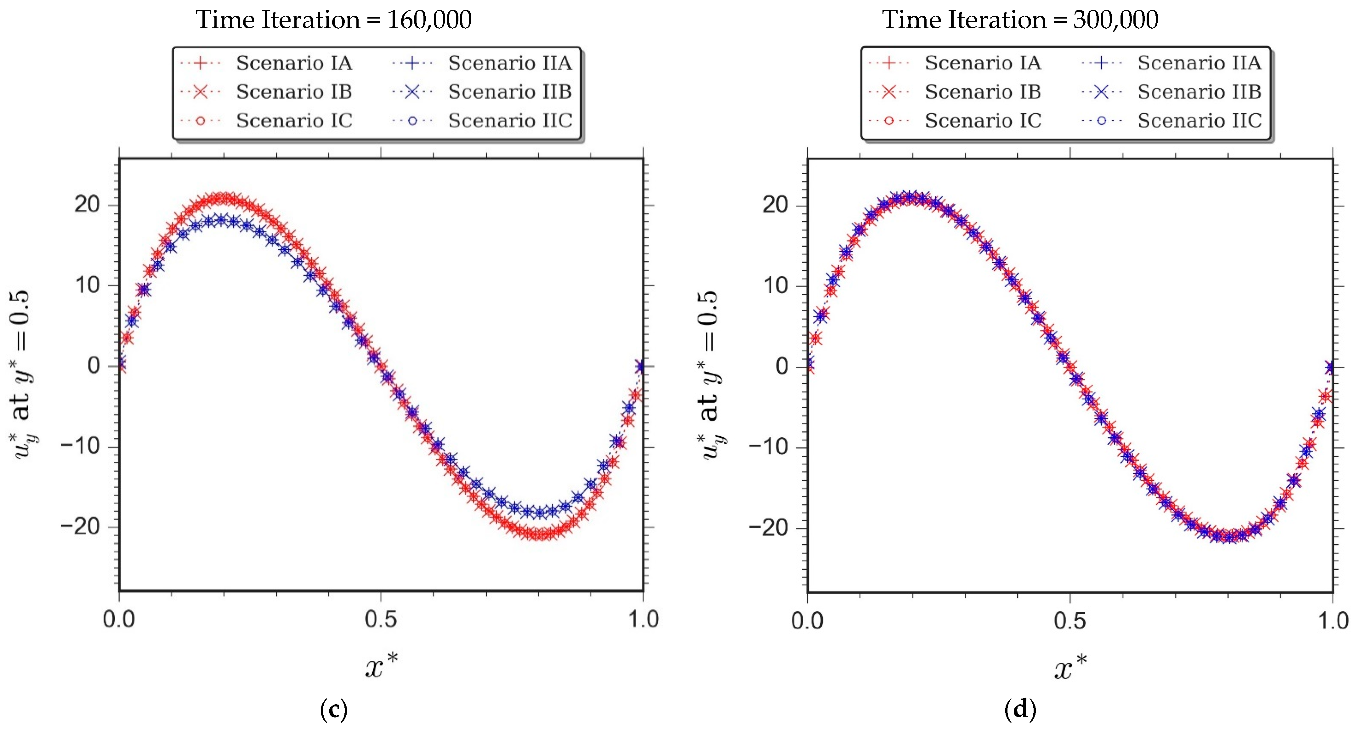
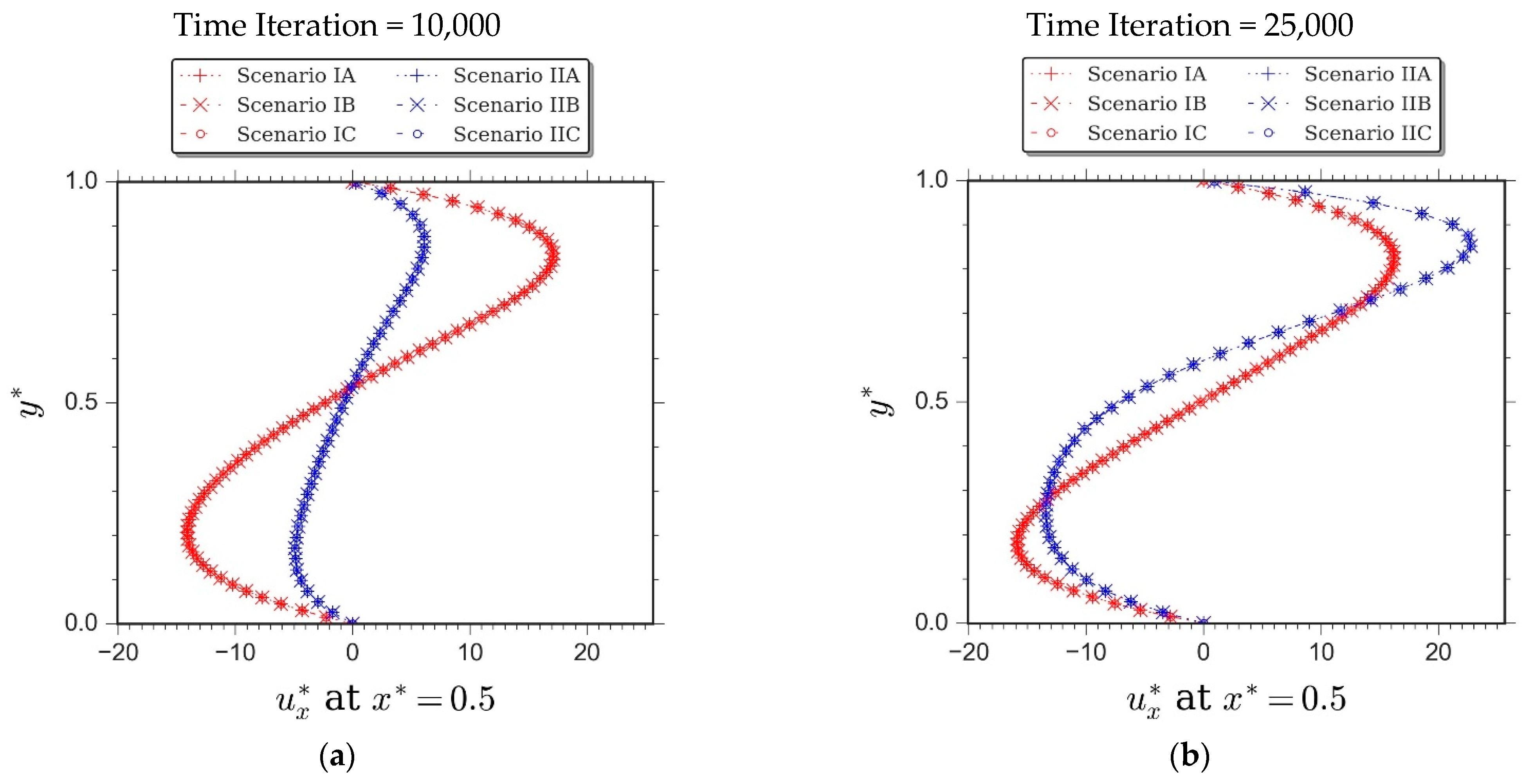
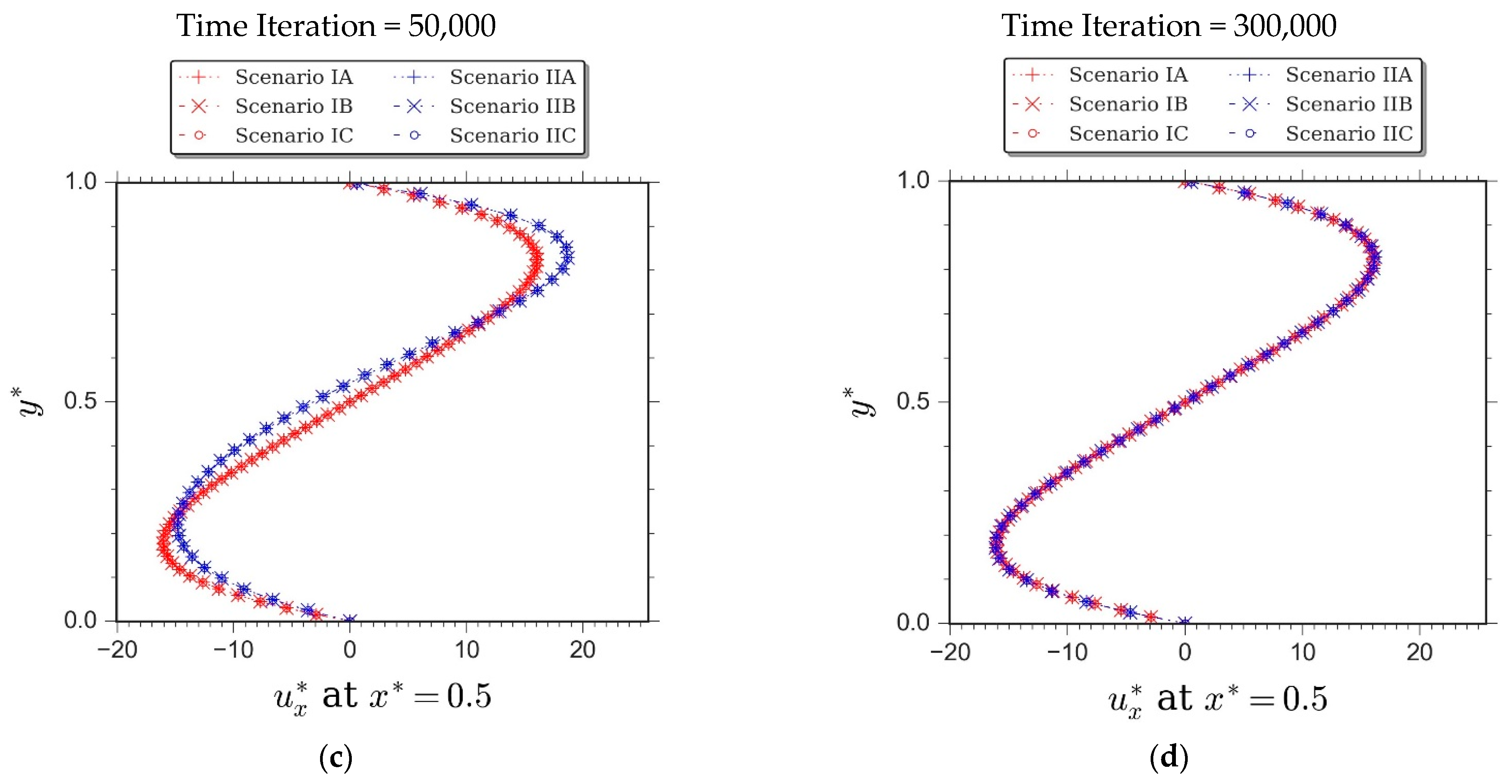
5.1. Simulation of Natural Convection in a Differentially-Heated Cavity

Figure 1 schematized the physical configuration of natural convection in a differentially-heated enclosure.
The entire domain was assumed filled with an inert fluid. The vertical walls of the cavity were characterised by contrasting thermal conditions. The left-border was considered hot ( T hot ) while the opposite wall was assumed cold ( T cold ). On the other hand, the horizontal boundaries were set to be perfectly insulated. For the fluid substance, the non-equilibrium bounce-back (NEBB) technique [19] was adopted upon all the corresponding perimeters, including the four corners. The NEBB method defines the unknown fluid populations at the boundaries from the known populations by evaluating the non-equilibrium condition of the normal populations at local boundary sites.
The non-equilibrium condition at the boundary wall satisfies the following remark:
ζ i ¯ f i ¯ e q = ζ i f i e q ξ i α N α ,
where N α notifies the momentum correction factor due to inclusion of the external forcing term into the generic Boltzmann expression of the fluid populations. The subscript symbol i ¯ specifies the opposite direction of i . Parameter ζ i was defined as follows:
ζ i = { f i , for   scenario   IA ,   IB   and   IC f ¯ i , for   scenario   IIA ,   IIB   and   IIC .
Meanwhile, for the thermal population, the anti-bounce-back (ABB) [2] and central finite difference [20] strategies were administered upon the vertical and horizontal boundaries, respectively.
ABB technique was administered by adopting the following relationship for the associated boundary walls:
g i ¯ ( x boundary , t + Δ t ) = g i * ( x boundary , t ) + 2 z i T wall ,
where g i * depicts thermal populations after collision and T wall notifies the prescribed temperature condition at particular boundary wall. To accomplish a valid comparison, numerical simulations for all the considered LBM scenarios were accomplished under similar hydrodynamic relaxation time ( τ υ = 0 . 6 ) and Mach number ( Ma = 0 . 1 ) conditions.
Thereupon, the average Nusselt number Nu was appointed as the dimensionless property that represents the heat transfer performance of each concomitant LBM scheme. This property abides to the following description:
N u = 1 + ( u x * Θ Θ hot Θ cold ) ,
where u x * Θ represents the average of the product between the dimensionless horizontal velocity and the dimensionless temperature over the entire simulation domain. For the sake of validation, the associated steady-state flow profile from scenario IIB was selected as the representation to exhibit the final streamlines and isotherms from the corresponding heat and mass transport system.
Figure 2 exhibits the steady-state streamlines and isotherms from the selected LBM scenario. The corresponding streamlines and isotherms profiles demonstrate an excellent agreement with the literature [16,17,21,22]. It was found, however, that the results from the six associated LBM scenarios exhibit almost similar steady-state flow profiles. Therefore, every considered LBM scheme possesses similar qualification in delivering legitimate steady-state numerical solutions.
Table 3 outlines the principal steady-state numerical properties from distinct LBM schemes. The parameters were compared with the outcomes of finite difference method (FDM) [23] and finite element method (FEM) [24]. A closer look on Table 3 reveals that LBM scenarios, which adopt a second-order lattice BGK model (i.e., scenario IIA, IIB, and IIC) were capable of delivering better compliance with the benchmark solutions than the ones which comprise first-order lattice BGK scheme (i.e., scenario IA, IB, and IC).
Undoubtedly, the inclusion of higher-truncation order terms empowers the second-order lattice BGK scheme with superior numerical accuracy to the corresponding first-order counterpart. Contrastingly, trivial disparity in computing performance was observed upon implementation of different forcing models.
Recording the behaviour of specific parameters along the simulation process provides a way of uncovering additional key information regarding the computational capacity of the considered LBM schemes. Figure 3a shows the profiles of Nu from different LBM scenarios with the dimensional simulation time t appointed as the horizontal axis. Figure 3b illustrates similar profiles with dimensionless simulation time t * used as the corresponding horizontal axis. Both figures display the existence of striking contrast in the computational characteristics among distinct LBM scenarios.
As depicted in Figure 3a, the discrepancy was predominantly apparent when the simulations were performed in an unsteady-state period fashion. Altering the fashion from unsteady to steady state, the disparity either decreases gradually or was negligible (Figure 3a). Such discrepancy was in agreement with the physical properties outlined Table 3.
Figure 3a unveils essential information regarding the primary factors responsible for the observed discrepancy in computational performance of distinct LBM scenarios. It appears then that the different order of lattice BGK expression is the predominant factor that generates the observed disparity in computational characteristics of different LBM schemes. On the other hand, the contribution of distinct forcing strategies upon such disparity was found to be inconsequential. Figure 3a reveals further that LBM schemes, which administer second-order lattice BGK model (i.e., scenarios IIA, IIB, and IIC) exhibited slower progression towards steady-state condition than those schemes which implement first-order lattice BGK model (i.e., scenarios IA, IB, and IC).
However, when non-dimensional time t * was assimilated, the slower progression characteristic of the second-order schemes vanished. Figure 3b shows that the computational performance of the second-order lattice BGK schemes is proportional to the first-order scenarios. The profiles of dimensionless horizontal velocity u x * at the vertical mid-plane of the enclosure ( x * = 0.5 ) were displayed in Figure 4. Therein, the profiles of u x * demonstrate similar behaviour with the ones observed in Figure 3a.
Figure 5 displays the corresponding computational overhead from every considered LBM scenario. The scenario IIC was identified as the particular LBM scheme with the highest computational demand in modelling fluid flow and heat transfer in a differentially-heated cavity, therein.

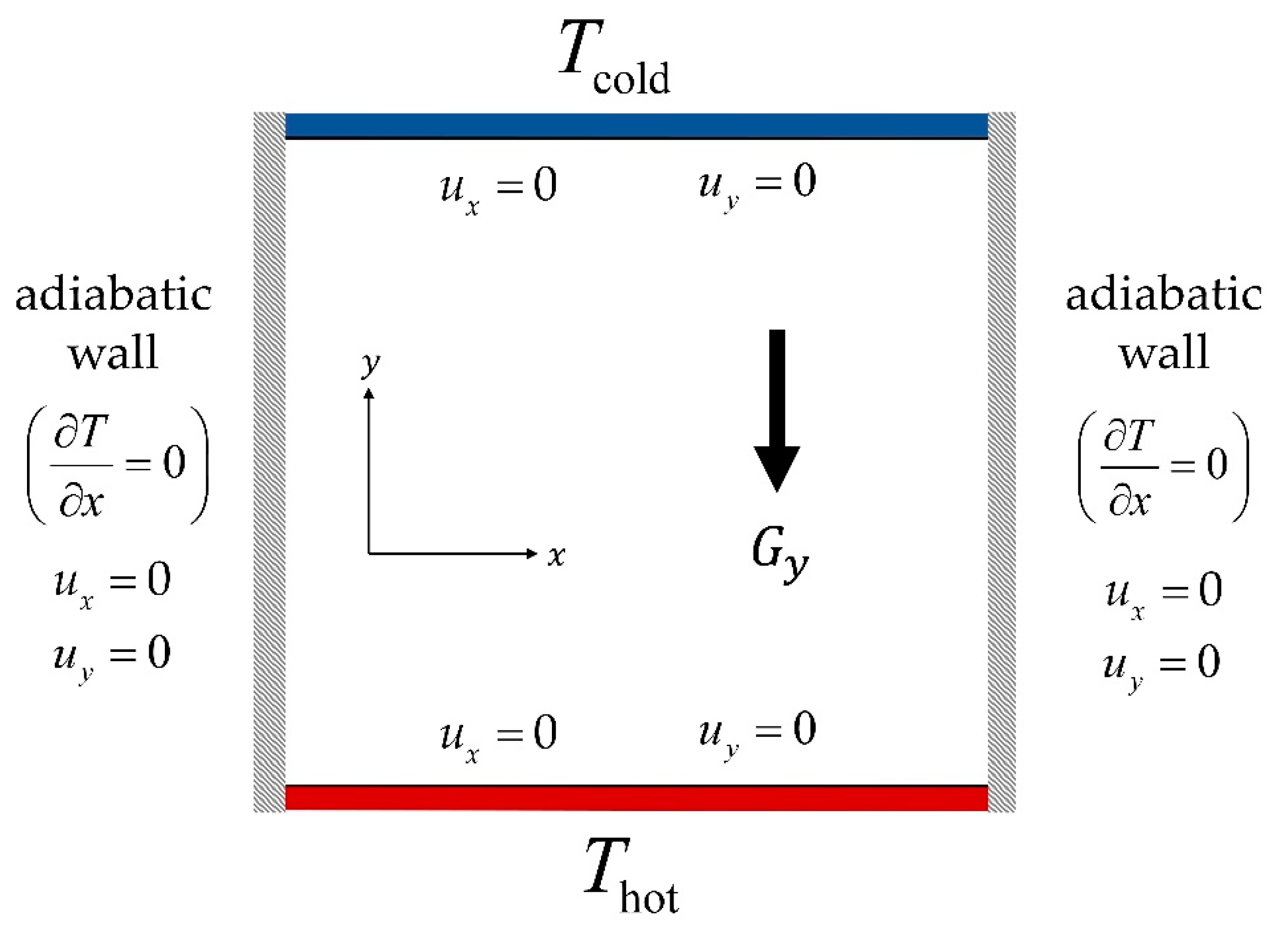
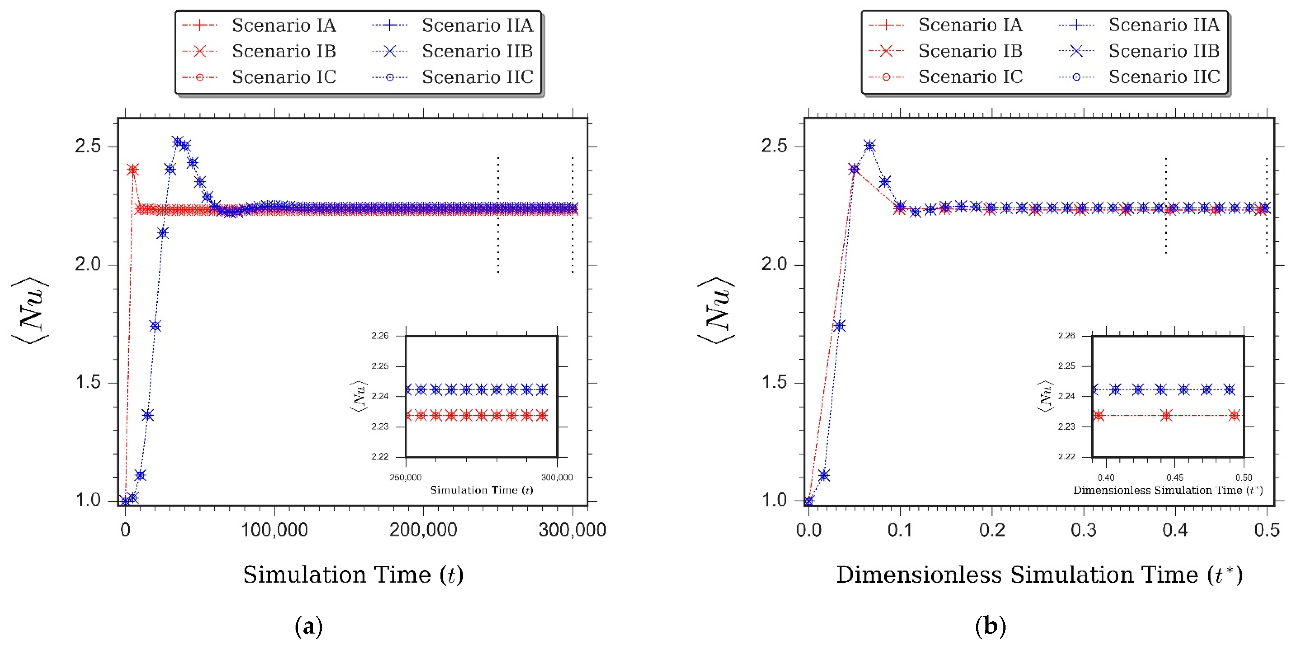
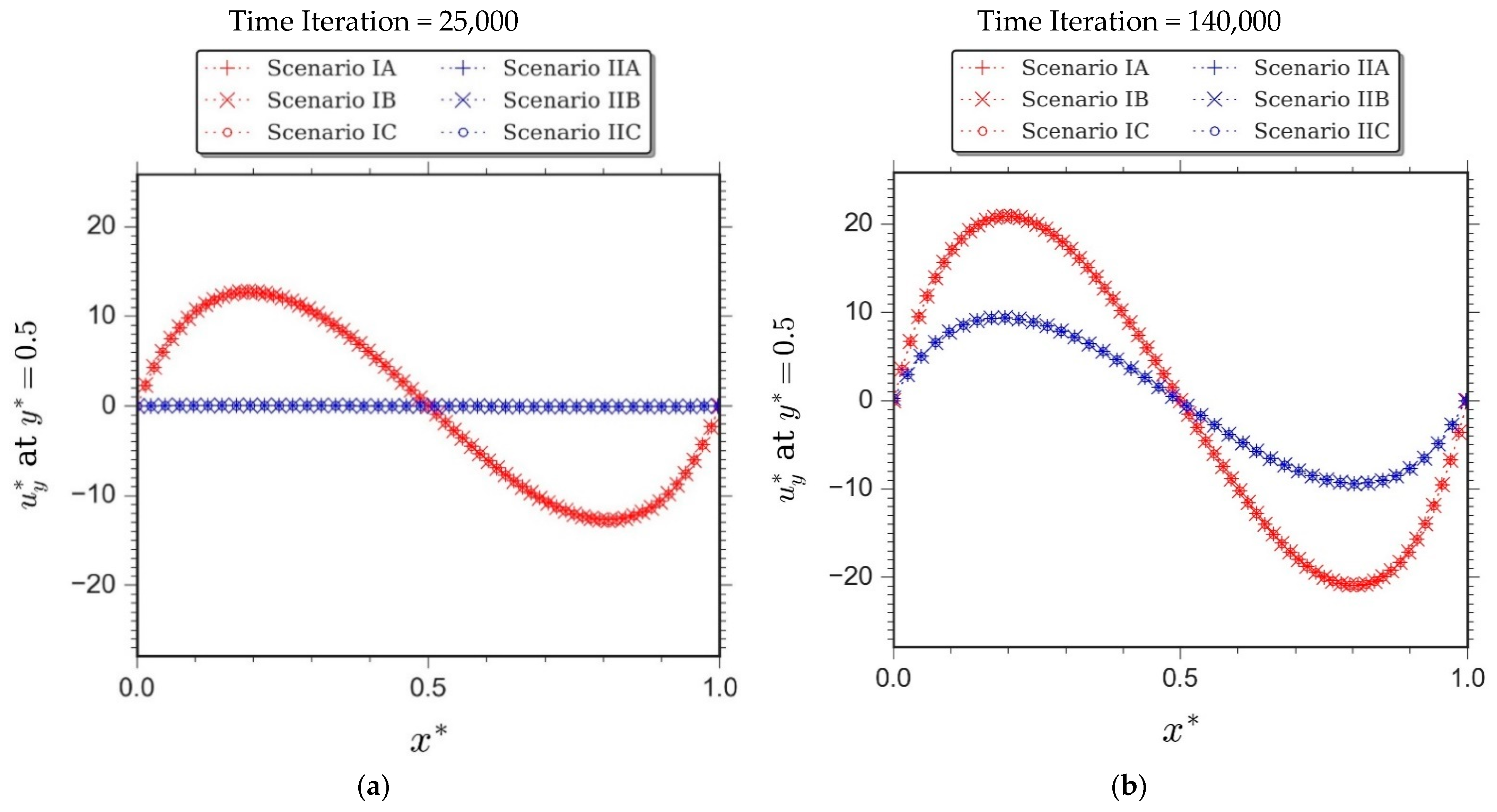
5.2. Simulation of Rayleigh-Bènard Convection

After undertaking evaluation regarding computational characteristics of distinct LBM scenarios upon simulating natural convection in a differentially-heated enclosure in the previous section, the current segment of the article aims at elucidating the capacity of disparate LBM scenarios while simulating the Rayleigh-Bènard convection (RBC) phenomena as illustrated in Figure 6.
Hot temperature conditions were imposed upon the horizontal bottom wall while the opposing top margin was set to occupy cold temperature. The vertical boundaries were set to be perfectly insulated. Boundary treatments were accomplished through adopting similar strategies with the erstwhile case of natural convection in a differentially-heated cavity. However, appropriate adjustments were necessary in order to account the appointed wall conditions in RBC configuration.
The contrasting driving force from buoyancy and gravitational attraction in the RBC system results in perpetual competition between the tendency of the flowing materials to move upward and downward, correspondingly. Such a situation enables the associated thermo-hydrodynamics phenomena to exhibit a number of plausibly distinct flow behaviours with variable convection roll patterns [25,26]. To mitigate such complexity, the present study assimilates infinitesimal disturbances into the corresponding physical system. These perturbation functions are described as
Θ initial ( x , y ) = Θ hot ( ( Θ hot Θ cold ) y N y ( 1 0.001 sin ( 2 π x N x ) ) )
ρ initial ( x , y ) = ρ ref ( 1 + β T ( Θ hot Θ cold ) y N y ( 1 0.001 sin ( 2 π x N x ) ) ) ,
where N x and N y designate the associated lattice nodes in the horizontal and vertical directions of the spatial coordinate, respectively.
The performance of heat transfer in RBC system was represented by the average Nusselt number at the hot wall, Nu 0 . The corresponding parameter was mathematically expressed as
N u 0 = 1 N x ( Θ hot Θ cold ) i = 1 N x q y ( i ) | y = 0 .
Here, q y specifies the local heat flux in vertical direction, defined as
q y = u y * Θ Θ y .
The last term on the right-hand side of the above formula denotes temperature gradient in a vertical direction.
Figure 7 presents the final streamlines and isotherms for RBC simulation with Ra = 10 4 and Pr = 0.71 . Similar to the former case of natural convection in a differentially-heated cavity, the steady-state flow profile from scenario IIB was selected for exhibition and validation purposes. The corresponding streamlines and isotherms displayed in Figure 7 were in excellent agreement with the earlier work of Ouertatani et al. [27]. Similarly to the former case of natural convection in a differentially-heated cavity, the obtained steady-state responses from distinct LBM schemes demonstrate identical flow profiles.
Nevertheless, minor discrepancy was observed in the captured Nu 0 solutions, which are summarized and compared with the outcomes of finite volume method (FVM) [27] in Table 4.
A better accuracy of Nu 0 solutions was obtained from the LBM scenarios which adopt a second-order lattice BGK model. The profiles of Nu 0 along the simulation process exhibited characteristics similar to those observed in the former natural convection case. Figure 8a illustrates further the behaviour of Nu 0 . A slow progression characteristic of the second-order lattice BGK schemes was observed that disappears as the horizontal axis is replaced by the associated dimensionless simulation time t * . Figure 9 shows the profiles of dimensionless vertical velocity u y * at the horizontal mid-plane of the cavity ( y * = 0 . 5 ) . Therein, similar computational behaviour was observed as the one prevailing in Figure 8a.
Figure 10 depicts the corresponding profiles of computational cost from every considered LBM schemes. Similar with the case of natural convection in a differentially-heated cavity, higher computational demand was displayed by the LBM schemes which adopt a second-order lattice BGK model.

6. Conclusions

Comprehensive evaluation regarding the efficacy of disparate Lattice Boltzmann Method (LBM) scenarios upon simulation of fluid flow and heat transfer phenomena were studied. The primary objective, herein addressed, was the evaluation of the plausible discrepancy in the computational characteristics of different LBM scenarios when simulating natural convection and heat transfer systems during the unsteady period of the flow. To fulfil the sought objective, the LBM schemes were tested upon two distinctive thermo-hydrodynamics systems, namely the natural convection in a differentially-heated cavity and the Rayleigh-Bènard convection. The key findings of this work are as follows:
1
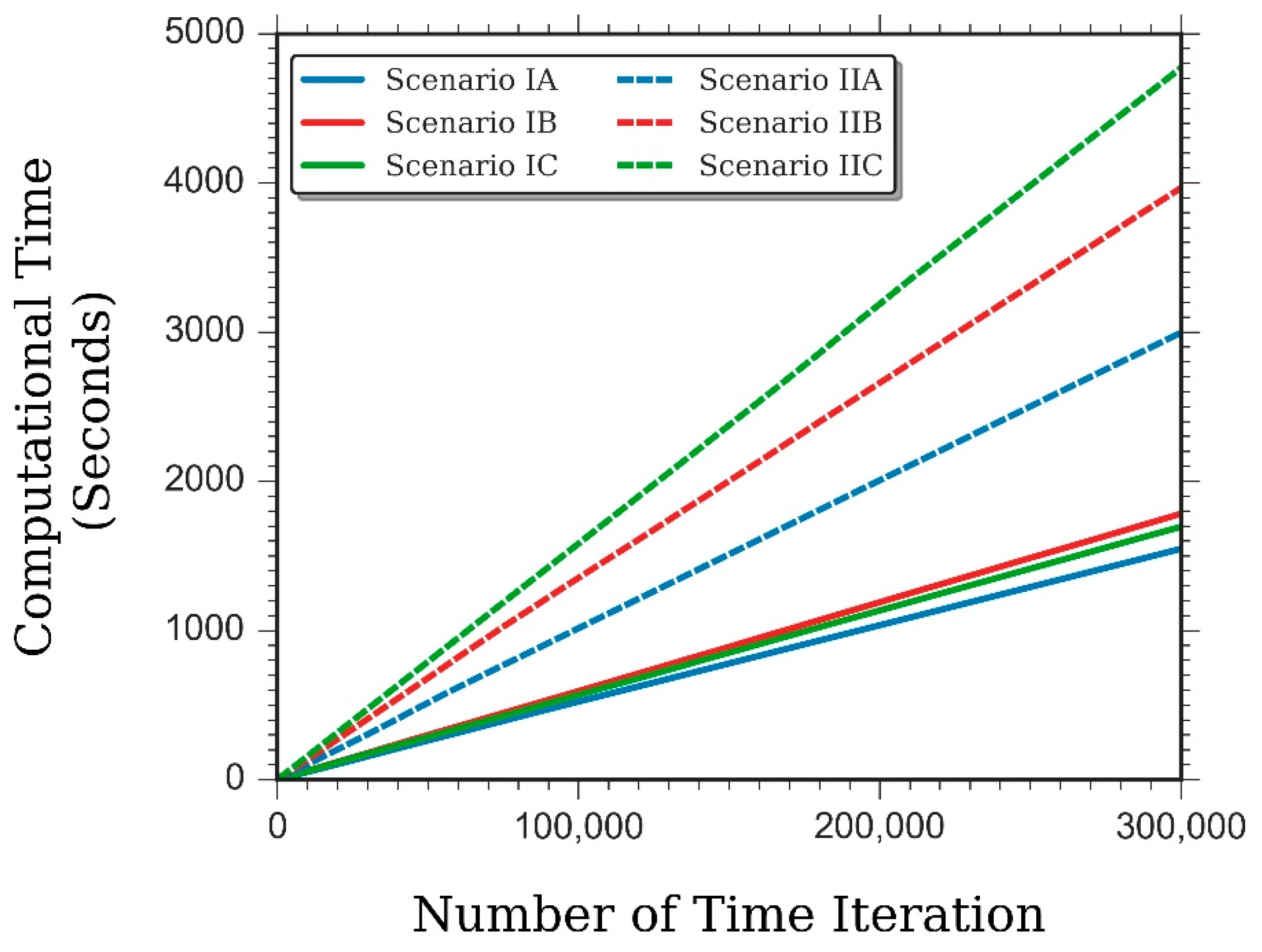
The presence of considerable discrepancy in computational characteristics of disparate LBM schemes was seen during the unsteady period of the simulation, which diminished gradually as the simulation advanced towards a steady-state condition.
2
Variation in the associated discrete lattice Boltzmann expression was identified as the predominant factor inherent to discrepancy in computational characteristics.
3
The contribution of distinct forcing models upon the heterogeneity in computational behaviour was found to be trivial.
4
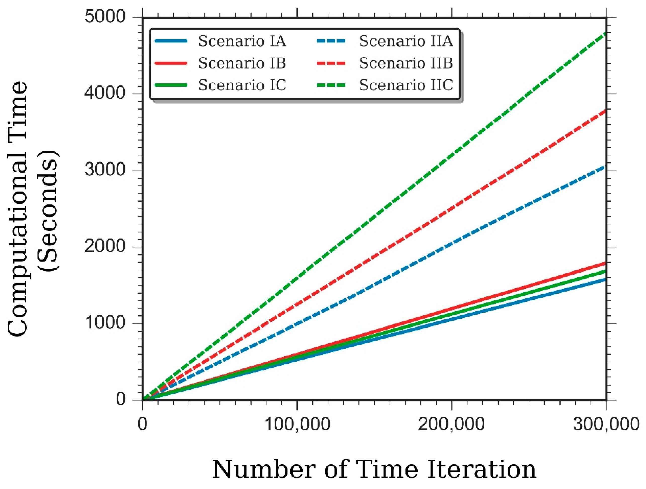
At a steady-state condition, the LBM schemes which administer a second-order lattice BGK model recovered better numerical accuracy than those scenarios which comprise a first-order lattice BGK model. However, the scheme is challenged by higher computational demand.

Author Contributions

A.D.H. devised the numerical methodology, conceptualisation, and composition of the present study, as well as developing the computer codes and preparing the original manuscript. K.S. contributes upon conceptualisation, supervision, reviewing, and editing the manuscript. Y.S. and R.N. provide supervision as well as editing the original manuscript. All authors have read and agreed to the published version of the manuscript.

Funding

This research received no external funding.

Data Availability Statement

This research does not accommodate data sharing option.

Acknowledgments

A.D.H. thanks the Japanese Ministry of Education, Culture, Sports, Science and Technology (MEXT) for bestowing financial support upon his doctoral training. The authors are indebted to Fajril Ambia of SKK Migas, Indonesia, for his auspicious suggestions during the development of computer codes of this study.

Conflicts of Interest

The authors declare no conflict of interest.

Nomenclature

ρ fluid   density ,   kg / m 3 ; x α spatial coordinates vector
T temperature, K; u α fluid   velocity ,   m / s
μ Fluid   dynamic   viscosity ;   kg / m s F α external   force ,   N
υ fluid   kinematic   viscosity ,   m 2 / s ; G α gravity   acceleration ,   m / s 2
D thermal   diffusivity ,   m 2 / s ; β T thermal   expansion   coefficient ,   K 1
T ref reference   temperature ,   K c s lattice speed of sound
T hot hot temperature, K; u char characteristic velocity
T cold cold temperature, K;NuNusselt number, dimensionless
h heat   transfer   coefficient ,   W / m 2 K ; Nu average Nusselt number for the entire simulation domain
c p specific   heat   capacity ,   J / k g K ; Nu 0 average Nusselt number at the hot wall
Lcharacteristic length, m;PrPrandtl number, dimensionless
Δ t simulation time step, lattice unit;RaRayleigh number, dimensionless
f i fluid population; Ma Mach number, dimensionless
f i e q equilibrium fluid population; x * dimensionless horizontal length
g i thermal population; y * dimensionless vertical length
g i e q equilibrium thermal population; u α * dimensionless fluid velocity
R i discrete forcing term; N x number of lattice nodes in the horizontal direction
w i weighting coefficients for fluid population; N y number of lattice nodes in the vertical direction
z i weighting coefficients for thermal population; q y local heat flux;
Greek symbols
ξ i α discrete velocity for fluid particles; τ υ relaxation time for fluid population
e i α discrete velocity for thermal particles; τ D relaxation time for thermal population
Θ dimensionless temperature; δ i j delta Kronecker
Θ hot dimensionless hot temperature; ϵ Knudsen number, dimensionless
Θ cold dimensionless cold temperature;
Subscript
i number of discrete velocities
α ,   β ,   γ direction of spatial coordinates (Einstein notation).

Appendix A. The Chapman-Enskog Analysis for Fluid Populations

The Chapman-Enskog analysis was commenced by defining the following expanded fractions:
ζ i = f i e q + ϵ ζ i ( 1 ) + ϵ 2 ζ i ( 2 ) t = ϵ t 1 + ϵ 2 t 2 ξ i α x α = ϵ ξ i α x α ( 1 ) + ϵ 2 ξ i α x α ( 2 ) R i = ϵ R i ( 1 ) .
In the above relationships, ϵ denotes small quantity which value lies within the order of Knudsen number and ζ i satisfies the remark described in Equation (33).
Adopting Taylor series expansion upon the generalized lattice Boltzmann expression for fluid components around equilibrium condition by taking ϵ as the expansion quantity returns the mathematical expressions for the first- and second-order expansion terms of the fluid density evolution equation, correspondingly depicted as
O ( ϵ ) : ( t 1 + ξ i α x α ( 1 ) ) f i e q = 1 σ ζ i ( 1 ) + φ R i ( 1 ) O ( ϵ 2 ) : ( t 2 + ξ i α x α ( 2 ) ) f i e q + ( t 1 + ξ i α x α ( 1 ) ) ( ( 1 Δ t 2 σ ) ζ i ( 1 ) + Δ t 2 φ R i ( 1 ) ) = 1 σ ζ i ( 2 ) ,
where O ( ϵ ) and O ( ϵ 2 ) specify respectively the first- and second-order expansion terms of the fluid density evolution equation. Parameters σ and φ occupy similar definitions as those provided in Equations (25) and (26), respectively.
Thereupon, expressions of moments of O ( ϵ ) and O ( ϵ 2 ) can be obtained as follows:
Moments of O ( ϵ ) :
i ( t 1 + ξ i α x α ( 1 ) ) f i e q = i ( 1 σ ζ i ( 1 ) + φ R i ( 1 ) ) i ξ i α ( t 1 + ξ i α x α ( 1 ) ) f i e q = i ξ i α ( 1 σ ζ i ( 1 ) + φ R i ( 1 ) ) i ξ i α ξ i β ( t 1 + ξ i α x α ( 1 ) ) f i e q = i ξ i α ξ i β ( 1 σ ζ i ( 1 ) + φ R i ( 1 ) )
Moments of O ( ϵ 2 ) :
i ( t 2 + ξ i α x α ( 2 ) ) f i e q + i ( t 1 + ξ i α x α ( 1 ) ) ( 1 Δ t 2 σ ) ζ i ( 1 ) + i ( t 1 + ξ i α x α ( 1 ) ) Δ t 2 φ R i ( 1 ) = 1 σ i ζ i ( 2 ) i ξ i α ( t 2 + ξ i α x α ( 2 ) ) f i e q + i ξ i α ( t 1 + ξ i α x α ( 1 ) ) ( 1 Δ t 2 σ ) ζ i ( 1 ) + i ξ i α ( t 1 + ξ i α x α ( 1 ) ) Δ t 2 φ R i ( 1 ) = 1 σ i ξ i α ζ i ( 2 ) .
Subsequently, the expressions for the three particular moments, namely the moments of the discrete forcing terms R i , the moments of the equilibrium density population f i e q and the moments of the expanded population ζ i have to be configured. Table A1 summarizes the expressions of forcing moments.
Table A1. Mathematical expressions for the moments of the discrete forcing terms R i for the three considered forcing schemes.
Forcing ModelZeroth-Order Moment
( i R i )
First-Order Moment
( i ξ i α R i )
Second-Order Moment
( i ξ i α ξ i β R i )
Luo (Equation (14))0 F α 0
Guo, et al. (Equation (15))0 F α F α u β + u α F β
Kupershtokh, et al. (Equation (16))0 F α F α u β + u α F β + 1 ρ ( F α F β )
The expressions for the moments of f i e q and ζ i were obtained accordingly as:
Moments of f i e q :
i f i e q = i ζ i + m Δ t i R i = ρ i ξ i α f i e q = i ξ i α ζ i + m Δ t i ξ i α R i = ρ u α i ξ i α ξ i β f i e q = i ξ i α ξ i β ζ i + m Δ t i ξ i α ξ i β R i = ρ u α u β + ρ c s 2 δ α β i ξ i α ξ i β ξ i γ f i e q = i ξ i α ξ i β ξ i γ ζ i + m Δ t i ξ i α ξ i β ξ i γ R i = ρ c s 2 ( u α δ β γ + u β δ α γ + u γ δ α β )
Moments of ζ i :
i ζ i ( 1 ) = m Δ t i R i ( 1 ) ; i ζ i ( 2 ) = 0 i ξ i α ζ i ( 1 ) = m Δ t i ξ i α R i ( 1 ) ; i ξ i α ζ i ( 2 ) = 0 i ξ i α ξ i β ζ i ( 1 ) = m Δ t i ξ i α ξ i β R i ( 1 ) ; i ξ i α ξ i β ζ i ( 2 ) = 0 i ξ i α ξ i β ξ i γ ζ i ( 1 ) = m Δ t i ξ i α ξ i β ξ i γ R i ( 1 ) ; i ξ i α ξ i β ξ i γ ζ i ( 2 ) = 0 .
Substituting the expressions of R i , f i e q and ζ i moments into Equations (A3) and (A4), the following remarks emerged:
ρ t 1 + x α ( 1 ) ( ρ u α ) = 0
t 1 ( ρ u α ) + x β ( 1 ) ( ρ u α u β + ρ c s 2 δ α β ) = ( φ + m Δ t σ ) i ξ i α R i ( 1 )
t 1 ( ρ u α u β + ρ c s 2 δ α β ) = x γ ( 1 ) ( ρ c s 2 u α δ β γ + ρ c s 2 u β δ α γ + ρ c s 2 u γ δ α β ) + ( φ + m Δ t σ ) i ξ i α ξ i β R i ( 1 )
ρ t 2 + x α ( 2 ) ( ρ u α ) = t 1 i R i ( 1 ) ( m Δ t m ( Δ t ) 2 2 σ Δ t 2 φ ) + x α ( 1 ) i ξ i α R i ( 1 ) ( m Δ t m ( Δ t ) 2 2 σ Δ t 2 φ )
t 2 ( ρ u α ) + x β ( 2 ) ( ρ u α u β + ρ c s 2 δ α β ) = t 1 i ξ i α R i ( 1 ) ( m Δ t m ( Δ t ) 2 2 σ Δ t 2 φ ) + x β ( 1 ) i ξ i α ξ i β R i ( 1 ) ( m Δ t m ( Δ t ) 2 2 σ Δ t 2 φ ) ,
where m occupies similar description as the one presented in Equation (24). Combining Equations (A7)–(A11) as well as substituting expressions of forcing moments from Table A1, the macroscopic hydrodynamics relationships of Equations (21) and (22) were restored. The residual fractions prevailed in the recovered hydrodynamics equations from each considered LBM scenarios were summarized in Table 2.

Appendix B. The Chapman-Enskog Analysis for Thermal Populations

For the thermal populations, the Chapman-Enskog analysis was performed following similar fashion as in the preceding analysis for the fluid components. However, the discrete velocity of thermal particles e i α was used instead of velocity of fluid particles ξ i α . The expanded terms for the thermal population occupy the following descriptions:
g i = g i e q + ϵ g i ( 1 ) + ϵ 2 g i ( 2 ) t = ϵ t 1 + ϵ 2 t 2 e i α x α = ϵ e i α x α ( 1 ) + ϵ 2 e i α x α ( 2 ) .
Executing similar fashion of Taylor series expansion upon the generalized lattice Boltzmann expression for the thermal particles produces the corresponding remarks:
O ( ϵ ) : ( t 1 + e i α x α ( 1 ) ) g i e q = 1 τ D g i ( 1 ) O ( ϵ 2 ) : ( t 2 + e i α x α ( 2 ) ) g i e q + ( t 1 + e i α x α ( 1 ) ) ( 1 Δ t 2 τ D ) g i ( 1 ) = 1 τ D g i ( 2 ) .
The corresponding moments of O ( ϵ ) and O ( ϵ 2 ) terms can be configured as follows:
Moments of O ( ϵ ) :
i ( t 1 + e i α x α ( 1 ) ) g i e q = i ( 1 τ D g i ( 1 ) ) i e i α ( t 1 + e i α x α ( 1 ) ) g i e q = i e i α ( 1 τ D g i ( 1 ) )
Moments of O ( ϵ 2 ) :
i ( t 2 + e i α x α ( 2 ) ) g i e q + i ( t 1 + e i α x α ( 1 ) ) ( 1 Δ t 2 τ D ) g i ( 1 ) = i ( 1 τ D g i ( 2 ) ) .
The moments of the thermal equilibrium population g i e q occupy the following definitions:
i g i e q = T i e i α g i e q = T u α i e i α e i β g i e q = T c s 2 δ α β + T u α u β .
Substituting Formula (A16) into Equations (A14) and (A15), the following expressions prevailed:
T t 1 + x α ( 1 ) ( T u α ) = 0
T t 2 + x α ( 2 ) ( T u α ) = c s 2 ( τ D Δ t 2 ) ( x α ( 1 ) x α ( 1 ) ( T ) + 1 c s 2 t 1 x α ( 1 ) ( T u α ) ) + ( τ D Δ t 2 ) x α ( 1 ) x β ( 1 ) ( T u α u β ) .
Combining Equations (A17) and (A18), the macroscopic heat equation depicted by Equation (23) was recovered.

References

  1. He, X.; Doolen, G.D. Thermodynamic foundations of kinetic theory and lattice Boltzmann models for multiphase flows. J. Stat. Phys. 2002, 107, 309–328. [Google Scholar] [CrossRef]
  2. Kruger, T.; Kusumaatmaja, H.; Kuzmin, A.; Shardt, O.; Goncalo, S.; Viggen, E.M. The Lattice Boltzmann Method, Principles and Practice; Springer: Cham, Switzerland, 2017; ISBN 9783319446479. [Google Scholar]
  3. Trouette, B. Lattice Boltzmann simulations of a time-dependent natural convection problem. Comput. Math. Appl. 2013, 66, 1360–1371. [Google Scholar] [CrossRef]
  4. Mezrhab, A.; Amine Moussaoui, M.; Jami, M.; Naji, H.; Bouzidi, M. Double MRT thermal lattice Boltzmann method for simulating convective flows. Phys. Lett. Sect. A Gen. Solid State Phys. 2010, 374, 3499–3507. [Google Scholar] [CrossRef]
  5. Jami, M.; Moufekkir, F.; Mezrhab, A.; Fontaine, J.P.; Bouzidi, M. New thermal MRT lattice Boltzmann method for simulations of convective flows. Int. J. Sci. 2016, 100, 98–107. [Google Scholar] [CrossRef]
  6. Ubertini, S.; Asinari, P.; Succi, S. Three ways to lattice Boltzmann: A unified time-marching picture. Phys. Rev. E-Stat. Nonlinear Soft Matter Phys. 2010, 81, 1–11. [Google Scholar] [CrossRef] [Green Version]
  7. Silva, G.; Semiao, V. First and Second-order forcing expressions in a lattice Boltzmann method reproducing isothermal hydrodynamics in artificial compressibility form. J. Fluid Mech. 2012, 698, 282–303. [Google Scholar] [CrossRef]
  8. Guo, Z.; Zheng, C.; Shi, B. Discrete lattice effects on the forcing term in the lattice Boltzmann method. Phys. Rev. E-Stat. Phys. Plasmas Fluids Relat. Interdiscip. Top. 2002, 65, 6. [Google Scholar] [CrossRef]
  9. Luo, L.S. Theory of the lattice Boltzmann method: Lattice Boltzmann models for nonideal gases. Phys. Rev. E-Stat. Phys. Plasmas Fluids Relat. Interdiscip. Top. 2000, 62, 4982–4996. [Google Scholar] [CrossRef] [PubMed]
  10. He, X.; Chen, S.; Doolen, G.D. A novel thermal model for the lattice Boltzmann method in incompressible limit. J. Comput. Phys. 1998, 146, 282–300. [Google Scholar] [CrossRef]
  11. Guo, Z.; Zhao, T.S. Lattice Boltzmann model for incompressible flows through porous media. Phys. Rev. E-Stat. Phys. Plasmas Fluids Relat. Interdiscip. Top. 2002, 66, 1–9. [Google Scholar] [CrossRef] [PubMed]
  12. Kupershtokh, A.L.; Medvedev, D.A.; Karpov, D.I. On equations of state in a lattice Boltzmann method. Comput. Math. Appl. 2009, 58, 965–974. [Google Scholar] [CrossRef] [Green Version]
  13. Mohamad, A.A.; Kuzmin, A.A. Critical evaluation of force term in lattice Boltzmann method, natural convection problem. Int. J. Heat Mass Transf. 2010, 53, 990–996. [Google Scholar] [CrossRef]
  14. Krivovichev, G.V. Stability analysis of body force action models used in the single-relaxation-time single-phase lattice Boltzmann method. Appl. Math. Comput. 2019, 348, 25–41. [Google Scholar] [CrossRef]
  15. Zheng, L.; Zheng, S.; Zhai, Q. Analysis of force treatment in lattice Boltzmann equation method. Int. J. Heat Mass Transf. 2019, 139, 747–750. [Google Scholar] [CrossRef]
  16. Mayne, D.A.; Usmani, A.S.; Crapper, M. H-adaptive finite element solution of high Rayleigh number thermally driven cavity problem. Int. J. Numer. Methods Heat Fluid Flow 2000, 10, 598–615. [Google Scholar] [CrossRef] [Green Version]
  17. Du, R.; Liu, W. A new multiple-relaxation-time lattice Boltzmann method for natural convection. J. Sci. Comput. 2013, 56, 122–130. [Google Scholar] [CrossRef]
  18. He, X.; Luo, L.S. Theory of the lattice Boltzmann method: From the Boltzmann equation to the lattice Boltzmann equation. Phys. Rev. E-Stat. Phys. Plasmas Fluids Relat. Interdiscip. Top. 1997, 55, 6811–6820. [Google Scholar] [CrossRef] [Green Version]
  19. Zou, Q.; He, X. On pressure and velocity boundary conditions for the lattice Boltzmann BGK model. Phys. Fluids 1997, 9, 1591–1596. [Google Scholar] [CrossRef] [Green Version]
  20. Shu, C.; Peng, Y.; Chew, Y.T. Simulation of natural convection in a square cavity by Taylor series expansion and least squares-based lattice Boltzmann method. Int. J. Mod. Phys. C 2002, 13, 1399–1414. [Google Scholar] [CrossRef] [Green Version]
  21. Dixit, H.N.; Babu, V. Simulation of high Rayleigh number natural convection in a square cavity using the lattice Boltzmann method. Int. J. Heat Mass Transf. 2006, 49, 727–739. [Google Scholar] [CrossRef]
  22. Yu, P.X.; Tian, Z.F. Compact computations based on a stream-function-velocity formulation of two-dimensional steady laminar natural convection in a square cavity. Phys. Rev. E-Stat. Nonlinear Soft Matter Phys. 2012, 85, 1–12. [Google Scholar] [CrossRef] [PubMed]
  23. De Vahl Davis, G. Natural convection of air in a square cavity: A bench mark numerical solution. Int. J. Numer. Methods Fluids 1983, 3, 249–264. [Google Scholar] [CrossRef]
  24. Syrjälä, S. Higher order penalty-galerkin finite element approach to laminar natural convection in a square cavity. Numer. Heat Transf. Part A Appl. 1996, 29, 197–210. [Google Scholar] [CrossRef]
  25. Goldhirsch, I.; Pelz, R.B.; Orszag, S.A. Numerical simulation of thermal convection in a two-dimensional finite box. J. Fluid Mech. 1989, 199, 1–28. [Google Scholar] [CrossRef]
  26. Shan, X. Simulation of Rayleigh-Bénard convection using a lattice Boltzmann method. Phys. Rev. E-Stat. Phy. Plasmas Fluids Relat. Interdiscip. Top. 1997, 55, 2780–2788. [Google Scholar] [CrossRef] [Green Version]
  27. Ouertatani, N.; Ben Cheikh, N.; Ben Beya, B.; Lili, T. Numerical simulation of two-dimensional Rayleigh-Bénard convection in an enclosure. Comptes Rendus Mécanique 2008, 336, 464–470. [Google Scholar] [CrossRef]
Figure 1. Domain configuration for two-dimensional natural convection in a differentially-heated cavity.
Computation 09 00065 g001
Figure 2. Steady-state flow characteristics of two-dimensional natural convection in a differentially-heated cavity for Ra = 10 4 , Pr = 0.71 , τ υ = 0.6 and Ma = 0.1 from scenario IIB, displaying (a) Streamlines and (b) Isotherms contour.
Computation 09 00065 g002
Figure 3. Profiles of average Nusselt number Nu from different LBM scenarios during the unsteady period up to the accomplishment of the steady-state condition of the natural convection a in differentially-heated cavity for Ra = 10 4 , Pr = 0.71 , τ υ = 0.6 , and Ma = 0.1 , showing computational behaviour with (a) dimensional simulation time t as the horizontal axis, and (b) dimensionless simulation time t * as the horizontal axis. Figure insets demonstrate the magnification of the computational characteristics in the steady-state region of the simulation.
Computation 09 00065 g003
Figure 4. Profiles of dimensionless horizontal velocity at the vertical mid-plane of the cavity upon different simulation periods of natural convection in differentially-heated cavity for Ra = 10 4 , Pr = 0.71 , τ υ = 0.6 and Ma = 0.1 , demonstrating condition at time iteration: (a) 10,000; (b) 25,000; (c) 50,000 and (d) 300,000.
Computation 09 00065 g004aComputation 09 00065 g004b
Figure 5. Computational overhead of disparate LBM schemes in modelling natural convection in a differentially-heated cavity with Ra = 10 4 , Pr = 0.71 , τ υ = 0.6 and Ma = 0.1 , starting from the unsteady period up to the accomplishment of the steady-state period.
Computation 09 00065 g005
Figure 6. Domain configuration for two-dimensional Rayleigh-Bènard convection with aspect ratio one.
Computation 09 00065 g006
Figure 7. Steady-state flow characteristics of Rayleigh-Bènard convection with aspect ratio = 1, Ra = 10 4 , Pr = 0.71 , τ υ = 0.6 , and Ma = 0.1 from scenario IIB, displaying (a) Streamlines and (b) Isotherms contour.
Computation 09 00065 g007
Figure 8. Profiles of average Nusselt number at the hot wall Nu 0 from different LBM scenarios during the unsteady period up to the accomplishment of steady-state condition of the Rayleigh-Bènard convection for aspect ratio = 1, Ra = 10 4 , Pr = 0.71 , τ υ = 0.6 , and Ma = 0.1 , showing computational behaviour with (a) dimensional simulation time t as the horizontal axis and (b) dimensionless simulation time t * as the horizontal axis. Figure insets display the magnification of the computational characteristics in the steady-state region of the simulation.
Computation 09 00065 g008
Figure 9. Profiles of dimensionless vertical velocity at the horizontal mid-plane of the cavity upon different simulation periods of Rayleigh-Bènard convection for aspect ratio = 1, Ra = 10 4 , Pr = 0.71 , τ υ = 0.6 , and Ma = 0.1 , demonstrating conditions at the following time iterations: (a) 25,000; (b) 140,000; (c) 160,000; and (d) 300,000.
Computation 09 00065 g009aComputation 09 00065 g009b
Figure 10. Computational overhead of disparate LBM schemes in modelling Rayleigh-Bènard convection with aspect ratio = 1, Ra = 10 4 , Pr = 0.71 , τ υ = 0.6 and Ma = 0.1 , starting from the transient period up to the accomplishment of the quasi-steady-state period.
Computation 09 00065 g010
Table 1. The plausible arrangements for simulating the buoyancy-driven natural convection flow with lattice Boltzmann method.
LBM SchemeLattice BGK Model for
Fluid Displacement
Discrete Forcing Model
IAFirst-Order
Lattice BGK Model
(Equation (7))
Luo [9] (Equation (14))
IBGuo et al. [8] (Equation (15))
ICKupershtokh et al. [12] (Equation (16))
IIASecond-Order
Lattice BGK Model
(Equation (8))
Luo [9] (Equation (14))
IIBGuo et al. [8] (Equation (15))
IICKupershtokh et al. [12] (Equation (16))
Table 2. The captured residual fractions in the recovered continuity and Navier-Stokes equations from every considered LBM scenarios.
LBM SchemeResidual Fractions
in the Restored
Continuity Equation
Residual Fractions in the Restored
Navier-Stokes Equation
IA Δ t 2 F α x α Δ t 2 F α t + ( τ υ Δ t 2 ) x β ( u α F β + F α u β )
IB Δ t 2 F α x α Δ t 2 F α t Δ t 2 x β ( u α F β + F α u β )
IC Δ t 2 F α x α Δ t 2 F α t Δ t 2 x β ( u α F β + F α u β ) τ υ x β ( F α F β ρ )
IIA0 ( τ ¯ υ Δ t 2 ) x β ( u α F β + F α u β )
IIB00
IIC0 ( τ ¯ υ Δ t 2 ) x β ( F α F β ρ )
Table 3. Steady-state properties of two-dimensional natural convection in a differentially-heated cavity for Ra = 10 4 , Pr = 0.71 , τ υ = 0.6 , and Ma = 0.1 , compared with solutions of finite difference method (FDM) [23] and finite element method (FEM) [24].
Simulation ParametersLBM Scheme (Present Study)FDM [23]FEM [24]
IAIBICIIAIIBIIC
Nu 2.23412.23392.23392.24242.24232.24242.2432.2448
Max   u x *   16.067816.061916.061916.174216.173216.174216.17816.1853
Max   u y *   19.392719.386419.386419.601119.599919.601119.61719.6316
Location   of   Max   u x *   0.81160.81160.81160.82040.82040.82040.8230.8230
Location   of   Max   u y *   0.11590.11590.11590.11890.11890.11890.1190.1188
at x * = 0.5 ; at y * = 0.5 .
Table 4. Average Nusselt number at the hot wall Nu 0 of the Rayleigh-Bènard convection system from distinct LBM schemes during the steady-state period of the flow for aspect ratio = 1, Ra = 10 4 , Pr = 0.71 , τ υ = 0.6 , and Ma = 0.1 compared with the outcome of the finite volume method (FVM) [27].
Simulation ParameterLBM Scheme (Present Study)FVM [27]
IAIBICIIAIIBIIC
Nu 0 2.16812.16842.16842.15542.15552.15542.1581
Publisher’s Note: MDPI stays neutral with regard to jurisdictional claims in published maps and institutional affiliations.

