Alternating Direction Implicit (ADI) Methods for Solving Two-Dimensional Parabolic Interface Problems with Variable Coefficients

Abstract

The matched interface and boundary method (MIB) and ghost fluid method (GFM) are two well-known methods for solving elliptic interface problems. Moreover, they can be coupled with efficient time advancing methods, such as the alternating direction implicit (ADI) methods, for solving time-dependent partial differential equations (PDEs) with interfaces. However, to our best knowledge, all existing interface ADI methods for solving parabolic interface problems concern only constant coefficient PDEs, and no efficient and accurate ADI method has been developed for variable coefficient PDEs. In this work, we propose to incorporate the MIB and GFM in the framework of the ADI methods for generalized methods to solve two-dimensional parabolic interface problems with variable coefficients. Various numerical tests are conducted to investigate the accuracy, efficiency, and stability of the proposed methods. Both the semi-implicit MIB-ADI and fully-implicit GFM-ADI methods can recover the accuracy reduction near interfaces while maintaining the ADI efficiency. In summary, the GFM-ADI is found to be more stable as a fully-implicit time integration method, while the MIB-ADI is found to be more accurate with higher spatial and temporal convergence rates.

1. Introduction

This work aims to develop alternating direction implicit (ADI) finite difference methods for solving a two-dimensional (2D) parabolic equation

$$\frac{\partial u}{\partial t}=\nabla ·(\beta \nabla u)+f=\frac{\partial }{\partial x}\left(\beta \frac{\partial }{\partial x}\right)u+\frac{\partial }{\partial y}\left(\beta \frac{\partial }{\partial y}\right)u+f,$$

(1)

over a rectangular domain $\mathsf{\Omega }\subset R^2$ with a Dirichlet boundary condition imposed on the boundary $\partial \mathsf{\Omega }$ and an initial condition defined at an initial time, i.e., $t=0$. Domain $\mathsf{\Omega }$ is split into two subdomains, an outer subdomain ${\mathsf{\Omega }}^{+}$ and an inner subdomain ${\mathsf{\Omega }}^{-}$, by a closed smooth curve, called an interface, such that $\mathsf{\Gamma }={\mathsf{\Omega }}^{-}\cap {\mathsf{\Omega }}^{+}$. In Equation (1), the diffusion coefficient $\beta (x,y)\ge {\beta }_0>0$ is assumed to be smooth in each subdomain, ${\mathsf{\Omega }}^{-}$ and ${\mathsf{\Omega }}^{+}$, but could be discontinuous across the interface $\mathsf{\Gamma }$, i.e., it is defined as a piecewise smooth function

$$\beta (x,y)=\left\{\begin{array}{cc}{\beta }^{+}(x,y),\hfill & \mathrm{i}\mathrm{f}(x,y)\in {\mathsf{\Omega }}^{+},\hfill \\ {\beta }^{-}(x,y),\hfill & \mathrm{i}\mathrm{f}(x,y)\in {\mathsf{\Omega }}^{-}.\hfill \end{array}\right.$$

(2)

Similarly, the source term $f(x,y)$ is assumed to be a piecewise smooth function. Due to the discontinuities of $\beta (x,y)$ and $f(x,y)$ on the interface, one can expect that the solution to Equation (1) is also a piecewise smooth function

$$u(t,x,y)=\left\{\begin{array}{cc}{u}^{+}(t,x,y),\hfill & \mathrm{i}\mathrm{f}(x,y)\in {\mathsf{\Omega }}^{+},\hfill \\ u^{-}(t,x,y),\hfill & \mathrm{i}\mathrm{f}(x,y)\in {\mathsf{\Omega }}^{-}.\hfill \end{array}\right.$$

(3)

Of course, $u^{-}$ and $u^{+}$ are not independent and should be related to each other on $\mathsf{\Gamma }$ by certain physical jump conditions. In this work, we assume the following general jump conditions

$$\left[u\right]:=u^{+}-u^{-}=\varphi (t,x,y),\left[\beta u_n\right]:={\beta }^{+}{u}_n^{+}-{\beta }^{-}{u}_n^{-}=\psi (t,x,y),\mathrm{f}\mathrm{o}\mathrm{r}(x,y)\in \mathsf{\Gamma },$$

(4)

in which the limiting value from each side of the interface has been taken for both $\beta$ and u. Here $\varphi$ and $\psi$ are known functions and n denotes the outer normal direction. A cartoon demonstration is provided in Figure 1. In addition, at an interface point, the tangential direction is denoted by $\tau$ and the angle formed by the normal direction n and the positive x-direction is denoted by $\theta$ in Figure 1.

Equations (1) and (4) yield a mathematical model known as the parabolic interface problem, which plays an important role in the fields of biophysics, engineering, material sciences, and so on, for studying physical quantities propagating across material interfaces between two media [1,2,3]. Exact solutions to parabolic interface problems are known only for a few simplified cases, while numerical approximations are usually demanded for most real-world applications. Because the physical solution could be non-smooth or even discontinuous across the interface, standard numerical algorithms are not capable of delivering accurate approximations. In the worst scenario, numerical computation could even fail to converge.

In the past few decades, a lot of efforts have been devoted towards developing accurate and efficient numerical methods to solve parabolic interface problems, based on both fitted and unfitted meshes, such as [4,5,6,7,8,9,10]. This study focuses on an unfitted mesh where a simple Cartesian grid is used and does not need to conform with the material interface. Consequently, carefully designed numerical procedures are required to account for jump conditions (4) in the numerical formulations so that numerical accuracy near the interface can be recovered. Such Cartesian grid interface algorithms have been successfully developed in many finite difference methods [4,6,8,10,11,12,13,14,15,16,17] and finite element methods [18,19,20].

Based on Cartesian grids, the alternating direction implicit (ADI) method [21,22] is known to be one of the most efficient algorithms for time integration of parabolic partial differential equations (PDEs). Such a high efficiency comes from two factors. First, for parabolic problems without material interfaces, the ADI method is usually unconditionally stable so that a large time step size can be used for saving the total number of time integration steps. Second, in each time step, a multidimensional system will be reduced to sets of independent one-dimensional (1D) subsystems, and the resulting matrices with tridiagonal structures can be efficiently inverted by using, for instance, the Thomas algorithm [23]. For a total spatial degree of freedom N, the complexity of ADI methods is of the order N, i.e., $O\left(N\right)$. This is much faster than other implicit step stepping schemes, in which the multidimensional system has to be solved by iterative algorithms. Indeed, due to its efficiency, the ADI method can also be applied as an algebraic solver, instead of a time stepper, for solving various PDEs [14,24,25]. For parabolic equations with variable coefficients, high accuracy ADI methods have been developed in [26].

The development of fast ADI methods for solving parabolic PDEs with material interfaces has attracted much research interest. The first study of this kind was carried out by Li and Mayo in 1993 [4], which combines the ADI with the immersed interface method (IIM) [27], yielding an IIM-ADI scheme. In solving a simplified parabolic interface problem with the material coefficient $\beta$ being a constant throughout the domain, the IIM-ADI scheme introduces some correction terms in the ADI formulation so that the accuracy near interfaces can be recovered back to second order. Later, this IIM-ADI scheme was applied to other parabolic PDEs [28,29]. For general jump conditions (4), the first ADI method that can not only maintain $O\left(N\right)$ efficiency but also produce second order spatial accuracy is the matched ADI (mADI) introduced by Zhao in 2015 [10]. Based on the matched interface and boundary (MIB) method [30,31] for general interface problems, a tensor product decomposition is conducted in the mADI to reduce jump conditions into 1D ones. Then these 1D conditions along Cartesian directions are enforced to secure a second order of convergence. A perturbed tridiagonal matrix is frequently encountered in the MIB-ADI computation, in which a few non-zero entries appear outside three diagonals due to interface treatments. An improved Thomas algorithm has been introduced in [10] for solving such systems with $O\left(N\right)$ complexity. The MIB-ADI method has been further formulated in the Peaceman-Rachford form [12] and for solving three-dimensional (3D) parabolic interface problems [13]. In [15], a popular interface algorithm–the ghost-fluid method (GFM) [32], is combined with the ADI for solving parabolic PDEs with constant coefficients. Comparing with the MIB-ADI scheme, the GFM-ADI is found to be more stable while being less accurate. Recently, another advance in this direction was presented in [14], in which a new IIM-ADI scheme is constructed for handling general jump conditions (4). This is achieved in an augmented IIM (AIIM) formulation by introducing auxiliary variables on the interface so that one can still solve an interface problem without material parameter $\beta$. The resulting AIIM-ADI scheme yields second order accuracy in both space and time.

Comparing with general interface algorithms for parabolic PDEs [6,8,11,16,17,18,19,20], the interface treatment in the ADI framework is more subtle. This is because the jump conditions (4) are prescribed in the normal direction so that the usual interface treatments naturally couple spatial derivatives in all Cartesian directions. However, in the ADI formulation, the jump conditions have to be enforced in a 1D manner, and such enforcement in different Cartesian directions shall be independent from each other. This is realized through two types of strategies in the existing studies. In the IIM-ADI methods [4,14], an argument formulation is employed, and simplified jump conditions can be satisfied multidimensionally through introducing corrections to standard central difference discretization of Laplacian operator. Then, the usual ADI splitting can be utilized to decompose the discrete Laplacian into 1D ones. In the MIB-ADI or mADI methods [10,12,13], the original jump conditions are decomposed in a tensor product manner to 1D, and the resulting 1D jump conditions are enforced in each alternating direction. The decomposition requires jump data in tangential directions at the future time step, say $t^{n+1}$. In order to avoid unwanted coupling, the tangential jumps are extrapolated by using function values at the current time step $t^n$ in the mADI methods. Thus, the MIB-ADI methods are semi-implicit in nature and are conditionally stable in general. We note that the AIIM-ADI scheme [14] is also conditionally stable. Fortunately, the stability constraints of MIB-ADI and IIM-ADI methods are still much less severe than those of the explicit time integration methods.

To the best of the authors’ acknowledge, all existing interface ADI methods concern only constant coefficient parabolic PDEs, and no efficient and accurate ADI method has been developed for variable coefficient parabolic interface problems. By using the augmented formulation, it may be possible to generalize the AIIM-ADI scheme [14] to solve variable coefficient problems. In fact, for elliptic interface problems, the generalization from constant coefficient to variable coefficient has been realized via the augmented formulation for both IIM [12] and the immersed finite element method [33]. Nevertheless, the ADI scheme is utilized as an algebraic solver in the AIIM-ADI method [14] and has to be calculated multiple times within each time step. This is less efficient than applying the ADI as a time stepper, in which the ADI procedure is executed only once per time step.

In this paper, the mADI method [10,12,13] will be generalized for solving variable coefficient parabolic interface problems, in which the ADI scheme serves as a time stepper. Away from the interface, the central difference discretization of Laplacian in divergence form will be employed, in which $\beta$ will be evaluated at half grid points. Near the interface, fictitious values for both u and $\beta$ will be assumed. Fictitious values of $\beta$ are obtained by using the diffusion coefficient definition from the other side, while those of u are solved from 1D jump conditions that are generated by the mADI procedure. In spatial discretization, we will examine both the first order GFM and second order MIB schemes for enforcing jump conditions. In time discretization, both the Douglas and Peaceman-Rachford ADI schemes will be employed as time steppers. More details about these ADI methods and their comparison will be provided in the following sections.

The rest of this work is organized as follows. In Section 2, the mADI procedure for solving variable coefficient parabolic interface problems will be presented. Details on spatial and temporal discretizations of the proposed MIB-ADI and GFM-ADI schemes will be offered. Numerical comparisons of four ADI methods are conducted on various examples in Section 3. Convergence rates and stability will be explored numerically as well, followed by concluding remarks in Section 4.

2. Theory and Algorithm

Standard finite different notations are adopted throughout this section to describe the proposed numerical methods for solving the parabolic interface problem governed by Equations (1) and (4). More specifically, we assume Equation (1) is solved for time $t\in [0,T]$ over a rectangular domain $\mathsf{\Omega }=[a,b]\times [c,d]$. The temporal domain $[0,T]$ is discretized into $N_t$ equally spaced subintervals by a uniform time step $\Delta t=\frac{T}{N_t}$, and the spatial domain is discretized by a uniform mesh size h in both x- and y- directions, yielding $N_x+1$ and $N_y+1$ grids in x- and y- directions, respectively, so that $h=\frac{b-a}{N_x}=\frac{d-c}{N_y}$. Numerical approximation to the exact solution $u(t_n,x_i,y_j)$ at grid $(x_i,y_j)$ and time instant $t_n$ is denoted by $u_{i,j}^n$ for all $i=0,1,\cdots ,N_x$, $j=0,1,\cdots ,N_y$ and $n=0,\cdots ,N_t$.

For the sake of simplicity, the superscript of $u_{i,j}^n$ is dropped when semi-discretized spatial methods are described in Section 2.1, and the subscripts of $u_{i,j}^n$ are dropped when semi-discretized temporal schemes are described in Section 2.2. Both super- and sub- scripts are then used when fully-discretized methods are demonstrated in Section 2.3.

2.1. Spatial Discretization

It is important to take jump conditions (4) into account when constructing finite difference formulas to approximate the two spatial derivatives, $\frac{\partial }{\partial x}\left(\beta \frac{\partial }{\partial x}\right)u$ and $\frac{\partial }{\partial y}\left(\beta \frac{\partial }{\partial y}\right)u$, in Equation (1). To this end, we denote corresponding finite difference operators as ${\delta }_{xx}\approx \frac{\partial }{\partial x}\left(\beta \frac{\partial }{\partial x}\right)$ and ${\delta }_{yy}\approx \frac{\partial }{\partial y}\left(\beta \frac{\partial }{\partial y}\right)$ and demonstrate their constructions by showing ${\delta }_{xx}{u}_{i,j}\left(\approx \frac{\partial }{\partial x}\left(\beta \frac{\partial }{\partial x}\right)u(x_i,y_j)\right)$ at a grid $(x_i,y_j)$ for $0<i<N_x$ on one grid line $y=y_j$. In a similar manner, ${\delta }_{yy}{u}_{i,j}\left(\approx \frac{\partial }{\partial y}\left(\beta \frac{\partial }{\partial y}\right)u(x_i,y_j)\right)$ at a grid $(x_i,y_j)$ on a grid line $x=x_i$ for $0<j<N_y$ can be obtained.

2.1.1. A Matched Interface and Boundary (MIB) Method

At a grid $(x_i,y_j)$ away from the interface $\mathsf{\Gamma }$, a second order approximation of ${\delta }_{xx}{u}_{i,j}$ can be constructed as

$$\begin{array}{ccc}\hfill {\delta }_{xx}{u}_{i,j}& =& \frac{{\left(\beta u_x\right)}_{i+\frac{1}{2},j}-{\left(\beta u_x\right)}_{i-\frac{1}{2},j}}{h}+O\left(h^2\right)\hfill \\ & =& \frac{{\beta }_{i+\frac{1}{2},j}{\left(u_x\right)}_{i+\frac{1}{2},j}-{\beta }_{i-\frac{1}{2},j}{\left(u_x\right)}_{i-\frac{1}{2},j}}{h}+O\left(h^2\right)\hfill \\ & =& \frac{{\beta }_{i+\frac{1}{2},j}\left(u_{i+1,j}-u_{i,j}\right)/h-{\beta }_{i-\frac{1}{2},j}\left(u_{i,j}-u_{i-1,j}\right)/h}{h}+O\left(h^2\right)\hfill \\ & =& \frac{{\beta }_{i+\frac{1}{2},j}{u}_{i+1,j}-\left({\beta }_{i+\frac{1}{2},j}+{\beta }_{i-\frac{1}{2},j}\right)u_{i,j}+{\beta }_{i-\frac{1}{2},j}{u}_{i-1,j}}{h^2}+O\left(h^2\right).\hfill \end{array}$$

(5)

However, Equation (5) must be adjusted to incorporate jump conditions (4) at grids near the interface $\mathsf{\Gamma }$, where jumps take place and the solution u is piecewise defined as in Equation (3). To this end, all grids on the grid line $y=y_j$ are classified into three categories. A grid $(x_I,y_j)$ is called a regular grid if three grids in the stencil $\{(x_{I-1},y_j),(x_I,y_j),(x_{I+1},y_j)\}$ are all on the same side, either the ${\mathsf{\Omega }}^{+}$- or ${\mathsf{\Omega }}^{-}$- side, of the interface $\mathsf{\Gamma }$. For instance, $(x_{i-1},y_j)$ and $(x_{i+2},y_j)$ are two regular grids in Figure 2a. A grid $(x_I,y_j)$ is called an irregular grid if one of its two adjacent grids, $(x_{I-1},y_j)$ or $(x_{I+1},y_j)$, is on the opposite side of the interface $\mathsf{\Gamma }$. In this case, the interface $\mathsf{\Gamma }$ cuts the grid line $y=y_j$ at a point $(x_{\mathsf{\Gamma }},y_j)$ where $x_{\mathsf{\Gamma }}\in (x_{i-1},x_i)$ or $x_{\mathsf{\Gamma }}\in (x_i,x_{i+1})$. Without loss of generality, we assume $(x_{\mathsf{\Gamma }},y_j)$ is off-grid and call it an irregular interface point. For instance, $(x_i,y_j)$ and $(x_{i+1},y_j)$ in Figure 2a are a pair of irregular grids. A grid $(x_I,y_j)$ is called a corner grid if both adjacent grids are on the opposite side of the interface $\mathsf{\Gamma }$ and the two associated interface points, denoted by $(x_{{\mathsf{\Gamma }}_1},y_j)$ and $(x_{{\mathsf{\Gamma }}_2},y_j)$, are called corner interface points. In this case, the left and right grids, $(x_{I-1},y_j)$ and $(x_{I+1},y_j)$, are also called corner grids. For instance, $\{(x_{i-1},y_j),(x_i,y_j),(x_{i+1},y_j)\}$ in Figure 2b are three corner grids.

After all grids on the grid line $y=y_j$ are properly classified, we propose to correct Equation (5) as

$${\delta }_{xx}{u}_{i,j}=\frac{{\overline{\beta }}_{i+\frac{1}{2},j}{\overline{u}}_{i+1,j}-\left({\overline{\beta }}_{i+\frac{1}{2},j}+{\overline{\beta }}_{i-\frac{1}{2},j}\right)u_{i,j}+{\overline{\beta }}_{i-\frac{1}{2},j}{\overline{u}}_{i-1,j}}{h^2}+O\left(h^2\right),$$

(6)

where

$${\overline{\beta }}_{i\pm \frac{1}{2},j}=\left\{\begin{array}{cc}{\beta }_{i\pm \frac{1}{2},j}^{+},\hfill & \mathrm{i}\mathrm{f}(x_i,y_j)\in {\mathsf{\Omega }}^{+}\hfill \\ {\beta }_{i\pm \frac{1}{2},j}^{-},\hfill & \mathrm{i}\mathrm{f}(x_i,y_j)\in {\mathsf{\Omega }}^{-},\hfill \end{array}\right.$$

(7)

and

$${\overline{u}}_{i\pm 1,j}=\left\{\begin{array}{cc}{u}_{i\pm 1,j},\hfill & \mathrm{i}\mathrm{f}(x_{i\pm 1},y_j)\mathrm{a}\mathrm{n}\mathrm{d}(x_i,y_j)\mathrm{are} \mathrm{on} \mathrm{the} \mathrm{same} \mathrm{side} \mathrm{of} \mathsf{\Gamma }\hfill \\ {\tilde{u}}_{i\pm 1,j},\hfill & \mathrm{if}(x_{i\pm 1},y_j)\mathrm{and}(x_i,y_j)\mathrm{are} \mathrm{on} \mathrm{the} \mathrm{opposite} \mathrm{side} \mathrm{of} \mathsf{\Gamma }.\hfill \end{array}\right.$$

(8)

The essential idea of Equation (6) is that when the involved function values of $\beta$ and u are from the opposite side of the interface, fictitious values, instead of the actual values, shall be employed, while at regular grids, Equation (6) is identical to Equation (5). The fictitious values of $\beta$ can be simply generated by applying the piecewise definition of the current side via Equation (2), but at a node on the other side. This is why in Equation (7), ${\overline{\beta }}_{i\pm \frac{1}{2},j}$ is always calculated according to the domain sign of the node $(x_i,y_j)$. In Equation (8), ${\tilde{u}}_{i\pm 1,j}$ denotes a fictitious value imposed at either irregular or corner grids. Such fictitious values are unknown and need to be approximated by using the jump conditions via the matched interface and boundary (MIB) method proposed in [10] and further discussed in [12,15]. One can view the fictitious values as approximations to the values of Equation (3) extended from the opposite side of the interface $\mathsf{\Gamma }$. For instance, if $(x_i,y_j)\in {\mathsf{\Omega }}^{-}$ is an irregular grid, ${\tilde{u}}_{i,j}\approx u^{+}(x_i,y_j)$ where $u^{+}(x_i,y_j)$ is obtained by extending $u^{+}$ from subdomain ${\mathsf{\Omega }}^{+}$ to subdomain ${\mathsf{\Omega }}^{-}$ and evaluated at $(x_i,y_j)$. Fictitious values play an important role and have significant impact on the accuracy and stability of the proposed method. A brief description is provided below to demonstrate how fictitious values are constructed via the MIB method, while one can find more detailed description in [10,15].

Let $(x_i,y_j)$ and $(x_{i+1},y_j)$ be a pair of irregular grids shown in Figure 2a, and we consider applying Equation (6) for calculating ${\delta }_{xx}{u}_{i,j}$ and ${\delta }_{xx}{u}_{i+1,j}$. Without loss of generality, it is assumed that $(x_{i-1},y_j)$ and $(x_i,y_j)$ are on the ${\mathsf{\Omega }}^{+}$-side while $(x_{i+1},y_j)$ is on the opposite ${\mathsf{\Omega }}^{-}$-side of the interface $\mathsf{\Gamma }$. A pair of fictitious values, ${\tilde{u}}_{i,j}$ and ${\tilde{u}}_{i+1,j}$, can be solved by considering jump conditions imposed at the interface $(x_{\mathsf{\Gamma }},y_j)$, where fictitious value ${\tilde{u}}_{i+1,j}$ is used for calculating ${\delta }_{xx}{u}_{i,j}$ and fictitious value ${\tilde{u}}_{i,j}$ is used for calculating ${\delta }_{xx}{u}_{i+1,j}$ by Equation (6). However, the jump condition $\psi =\left[\beta u_n\right]$ cannot be used immediately because it is on the normal direction n, which usually does not coincide with the x-direction. It must be converted to a jump condition in the x-direction, i.e., $\overline{\psi }:=\left[\beta u_x\right]$, before it can be used in numerical formations. As indicated in Zhao’s work [10], $\overline{\psi }$ can be expressed as

$$\begin{array}{ccc}\hfill \overline{\psi }& =& \psi cos\left(\theta \right)-sin\left(\theta \right)\left({\beta }^{+}-{\beta }^{-}\right)u_{\tau }^{+}-sin\left(\theta \right){\beta }^{-}{\varphi }_{\tau }\hfill \end{array}$$

(9)

$$\begin{array}{ccc}& =& \psi cos\left(\theta \right)-sin\left(\theta \right)\left({\beta }^{+}-{\beta }^{-}\right)u_{\tau }^{-}-sin\left(\theta \right){\beta }^{+}{\varphi }_{\tau },\hfill \end{array}$$

(10)

where ${\varphi }_{\tau }$ is the derivative of $\varphi$ along the tangential direction, and $u_{\tau }^{+}$ and $u_{\tau }^{-}$ are the tangential derivatives of u from the ${\mathsf{\Omega }}^{+}$- and ${\mathsf{\Omega }}^{-}$- sides of the interface, respectively. Equations (9) and (10) allow $\overline{\psi }$ to be calculated from either side of the interface $\mathsf{\Gamma }$. Moreover, one can see that all quantities involved on the right-hand sides of Equations (9) and (10) can be analytically obtained except that the two derivatives along the tangential direction $\tau$, i.e., $u_{\tau }^{+}$ and $u_{\tau }^{-}$, must be estimated via certain numerical procedures.

A new numerical procedure to approximate $u_{\tau }^{+}$ and $u_{\tau }^{-}$ will be proposed in the next subsection. At this moment, assuming either $u_{\tau }^{+}$ or $u_{\tau }^{-}$ has been numerically generated, the two jump conditions

$${\varphi }_{\mathsf{\Gamma },j}={\left[u\right]}_{\mathsf{\Gamma },j}={\left(u^{+}\right)}_{\mathsf{\Gamma },j}-{\left(u^{-}\right)}_{\mathsf{\Gamma },j},{\overline{\psi }}_{\mathsf{\Gamma },j}={\left[\beta u_x\right]}_{\mathsf{\Gamma },j}={\beta }_{\mathsf{\Gamma },j}^{+}{\left(u_x^{+}\right)}_{\mathsf{\Gamma },j}-{\beta }_{\mathsf{\Gamma },j}^{-}{\left(u_x^{-}\right)}_{\mathsf{\Gamma },j},$$

(11)

at the interface point $(x_{\mathsf{\Gamma }},y_j)$ shown in Figure 2a are ready to be used. Denoting the values of $\beta$ at $(x_{\mathsf{\Gamma }},y_j)$ as ${\beta }_{\mathsf{\Gamma },j}^{+}$ and ${\beta }_{\mathsf{\Gamma },j}^{-}$, a system of equations.

$$\begin{array}{c}{\displaystyle \stackrel{\approx {\left(u^{+}\right)}_{\mathsf{\Gamma },j}}{\overbrace{w_{i-1}^{0,+}{u}_{i-1,j}+w_i^{0,+}{u}_{i,j}+w_{i+1}^{0,+}{\tilde{u}}_{i+1,j}}}}\\ =\underset{\approx {\left(u^{-}\right)}_{\mathsf{\Gamma },j}}{\underbrace{w_i^{0,-}{\tilde{u}}_{i,j}+w_{i+1}^{0,-}{u}_{i+1,j}+w_{i+2}^{0,-}{u}_{i+2,j}}}+{\varphi }_{\mathsf{\Gamma },j}+O\left(h^2\right),\hfill \\ {\displaystyle {\beta }_{\mathsf{\Gamma },j}^{+}\stackrel{\approx {\left(u_x^{+}\right)}_{\mathsf{\Gamma },j}}{\overbrace{\left(w_{i-1}^{1,+}{u}_{i-1,j}+w_i^{1,+}{u}_{i,j}+w_{i+1}^{1,+}{\tilde{u}}_{i+1,j}\right)}}}\\ ={\beta }_{\mathsf{\Gamma },j}^{-}\underset{\approx {\left(u_x^{-}\right)}_{\mathsf{\Gamma },j}}{\underbrace{\left(w_i^{1,-}{\tilde{u}}_{i,j}+w_{i+1}^{1,-}{u}_{i+1,j}+w_{i+2}^{1,-}{u}_{i+2,j}\right)}}+{\overline{\psi }}_{\mathsf{\Gamma },j}+O\left(h^2\right),\hfill \end{array}$$

(12)

is constructed to be solved for ${\tilde{u}}_{i,j}$ and ${\tilde{u}}_{i+1,j}$ as linear combinations of $\{u_{i-1,j}$, $u_{i,j}$, $u_{i+1,j}$, $u_{i+2,j}$, ${\varphi }_{\mathsf{\Gamma },j}$, ${\overline{\psi }}_{\mathsf{\Gamma }}\}$. Weights ($w_{i-1}^{0,+}$, $w_{i-1}^{1,+}$ and so on) involved in (12) are pre-calculated by the Fornberg’s method [34] to maintain second order in all approximations. The representations of ${\tilde{u}}_{i,j}$ and ${\tilde{u}}_{i+1,j}$ are then used in Equation (6) for calculating ${\delta }_{xx}{u}_{i,j}$ and ${\delta }_{xx}{u}_{i+1,j}$.

In Figure 2b, jump conditions at the left and right corner interface points, $(x_{{\mathsf{\Gamma }}_1},y_j)$ and $(x_{{\mathsf{\Gamma }}_2},y_j)$, are taken into consideration at the same time so that a system of four equations can be obtained from jumps

$$\begin{array}{c}{\displaystyle {\varphi }_{{\mathsf{\Gamma }}_1,j}={\left[u\right]}_{{\mathsf{\Gamma }}_1,j},{\overline{\psi }}_{{\mathsf{\Gamma }}_1,j}={\left[\beta u_x\right]}_{{\mathsf{\Gamma }}_1,j},\mathrm{at} \mathrm{the} \mathrm{left} \mathrm{corner} (x_{{\mathsf{\Gamma }}_1},y_j)}\hfill \\ {\displaystyle {\varphi }_{{\mathsf{\Gamma }}_2,j}={\left[u\right]}_{{\mathsf{\Gamma }}_2,j},{\overline{\psi }}_{{\mathsf{\Gamma }}_2,j}={\left[\beta u_x\right]}_{{\mathsf{\Gamma }}_2,j},\mathrm{at} \mathrm{the} \mathrm{right} \mathrm{corner} (x_{{\mathsf{\Gamma }}_2},y_j),}\hfill \end{array}$$

in a similar manner. In order to accommodate the resulting system of equations, the MIB method suggests four fictitious values, ${\tilde{u}}_{i-2,j}$, ${\tilde{u}}_{i-1,j}$, ${\tilde{u}}_{i,j}$, and ${\tilde{u}}_{i+1,j}$, to be imposed and solved from

$$\begin{array}{c}\hfill {\displaystyle {\left(w_{{\mathsf{\Gamma }}_1}\right)}_{i-2}^{0,+}{u}_{i-2,j}+{\left(w_{{\mathsf{\Gamma }}_1}\right)}_{i-1}^{0,+}{u}_{i-1,j}+{\left(w_{{\mathsf{\Gamma }}_1}\right)}_i^{0,+}{\tilde{u}}_{i,j}+{\left(w_{{\mathsf{\Gamma }}_1}\right)}_{i+1}^{0,+}{u}_{i+1,j}+O\left(h^2\right)}\\ ={\left(w_{{\mathsf{\Gamma }}_1}\right)}_{i-2}^{0,-}{\tilde{u}}_{i-2,j}+{\left(w_{{\mathsf{\Gamma }}_1}\right)}_{i-1}^{0,-}{\tilde{u}}_{i-1,j}+{\left(w_{{\mathsf{\Gamma }}_1}\right)}_i^{0,-}{u}_{i,j}+{\left(w_{{\mathsf{\Gamma }}_1}\right)}_{i+1}^{0,-}{\tilde{u}}_{i+1,j}+{\varphi }_{{\mathsf{\Gamma }}_1,j},\hfill \\ \hfill {\displaystyle {\beta }_{{\mathsf{\Gamma }}_1,j}^{+}\left({\left(w_{{\mathsf{\Gamma }}_1}\right)}_{i-2}^{1,+}{u}_{i-2,j}+{\left(w_{{\mathsf{\Gamma }}_1}\right)}_{i-1}^{1,+}{u}_{i-1,j}+{\left(w_{{\mathsf{\Gamma }}_1}\right)}_i^{1,+}{\tilde{u}}_{i,j}+{\left(w_{{\mathsf{\Gamma }}_1}\right)}_{i+1}^{1,+}{u}_{i+1,j}\right)+O\left(h^2\right)}\\ ={\beta }_{{\mathsf{\Gamma }}_1,j}^{-}\left({\left(w_{{\mathsf{\Gamma }}_1}\right)}_{i-2}^{1,-}{\tilde{u}}_{i-2,j}+{\left(w_{{\mathsf{\Gamma }}_1}\right)}_{i-1}^{1,-}{\tilde{u}}_{i-1,j}+{\left(w_{{\mathsf{\Gamma }}_1}\right)}_i^{1,-}{u}_{i,j}+{\left(w_{{\mathsf{\Gamma }}_1}\right)}_{i+1}^{1,-}{\tilde{u}}_{i+1,j}\right)+{\overline{\psi }}_{{\mathsf{\Gamma }}_1,j},\hfill \\ \hfill {\displaystyle {\left(w_{{\mathsf{\Gamma }}_2}\right)}_{i-1}^{0,+}{u}_{i-1,j}+{\left(w_{{\mathsf{\Gamma }}_2}\right)}_i^{0,+}{\tilde{u}}_{i,j}+{\left(w_{{\mathsf{\Gamma }}_2}\right)}_{i+1}^{0,+}{u}_{i+1,j}+{\left(w_{{\mathsf{\Gamma }}_2}\right)}_{i+2}^{0,+}{u}_{i+2,j}+O\left(h^2\right)}\\ ={\left(w_{{\mathsf{\Gamma }}_2}\right)}_{i-2}^{0,-}{\tilde{u}}_{i-2,j}+{\left(w_{{\mathsf{\Gamma }}_2}\right)}_{i-1}^{0,-}{\tilde{u}}_{i-1,j}+{\left(w_{{\mathsf{\Gamma }}_2}\right)}_i^{0,-}{u}_{i,j}+{\left(w_{{\mathsf{\Gamma }}_2}\right)}_{i+1}^{0,-}{\tilde{u}}_{i+1,j}+{\varphi }_{{\mathsf{\Gamma }}_2,j},\hfill \\ \hfill {\displaystyle {\beta }_{{\mathsf{\Gamma }}_2,j}^{+}\left({\left(w_{{\mathsf{\Gamma }}_2}\right)}_{i-1}^{1,+}{u}_{i-1,j}+{\left(w_{{\mathsf{\Gamma }}_2}\right)}_i^{1,+}{\tilde{u}}_{i,j}+{\left(w_{{\mathsf{\Gamma }}_2}\right)}_{i+1}^{1,+}{u}_{i+1,j}+{\left(w_{{\mathsf{\Gamma }}_2}\right)}_{i+2}^{1,+}{u}_{i+2,j}\right)+O\left(h^2\right)}\\ ={\beta }_{{\mathsf{\Gamma }}_2,j}^{-}\left({\left(w_{{\mathsf{\Gamma }}_2}\right)}_{i-2}^{1,-}{\tilde{u}}_{i-2,j}+{\left(w_{{\mathsf{\Gamma }}_2}\right)}_{i-1}^{1,-}{\tilde{u}}_{i-1,j}+{\left(w_{{\mathsf{\Gamma }}_2}\right)}_i^{1,-}{u}_{i,j}+{\left(w_{{\mathsf{\Gamma }}_2}\right)}_{i+1}^{1,-}{\tilde{u}}_{i+1,j}\right)+{\overline{\psi }}_{{\mathsf{\Gamma }}_2,j}.\hfill \end{array}$$

(13)

for the case shown in Figure 2b where $w_{{\mathsf{\Gamma }}_1}$’s and $w_{{\mathsf{\Gamma }}_2}$’s are pre-calculated weights obtained at the left and right corner interface points, respectively. Solving the system of Equation (13) for ${\tilde{u}}_{i-2,j}$, ${\tilde{u}}_{i-1,j}$, ${\tilde{u}}_{i,j}$, and ${\tilde{u}}_{i+1,j}$ results in their representations in terms of $\{u_{i-2,j},u_{i-1,j},u_{i,j},u_{i+1,j},$$u_{i+2,j},{\varphi }_{{\mathsf{\Gamma }}_1,j},{\overline{\psi }}_{{\mathsf{\Gamma }}_1,j},{\varphi }_{{\mathsf{\Gamma }}_2,j},{\overline{\psi }}_{{\mathsf{\Gamma }}_2,j}\}$. Representations of three fictitious values, ${\tilde{u}}_{i-1,j}$, ${\tilde{u}}_{i,j}$, and ${\tilde{u}}_{i+1,j}$, are then used in Equation (6) for calculating ${\delta }_{xx}{u}_{i-1,j}$, ${\delta }_{xx}{u}_{i,j}$ and ${\delta }_{xx}{u}_{i+1,j}$.

The above discussions provide a second order accurate procedure to construct the finite difference approximation ${\delta }_{xx}u\approx \frac{\partial }{\partial x}\left(\beta \frac{\partial }{\partial x}\right)u$ at all internal grids on grid line $y=y_j$ for $j=1,\cdots ,N_y-1$. A similar produce can be carried out for constructing ${\delta }_{yy}\approx \frac{\partial }{\partial y}\left(\beta \frac{\partial }{\partial y}\right)u$ at all internal grids on grid line $x=x_i$ for $i=1,\cdots ,N_x-1$. More specifically, a formula analogous to Equation (6) is given by

$${\delta }_{yy}{u}_{i,j}=\frac{{\widehat{\beta }}_{i,j+\frac{1}{2}}{\widehat{u}}_{i,j+1}-\left({\widehat{\beta }}_{i,j+\frac{1}{2}}+{\widehat{\beta }}_{i,j-\frac{1}{2}}\right)u_{i,j}+{\widehat{\beta }}_{i,j-\frac{1}{2}}{\widehat{u}}_{i,j-1}}{h^2}+O\left(h^2\right),$$

(14)

and applied to all grids on grid line $x=x_i$ for $i=1,\cdots ,N_x-1$. Here

$${\widehat{\beta }}_{i,j+\frac{1}{2}}=\left\{\begin{array}{cc}{\beta }_{i,j+\frac{1}{2}}^{+},\hfill & \mathrm{i}\mathrm{f}(x_i,y_j)\in {\mathsf{\Omega }}^{+}\hfill \\ {\beta }_{i,j+\frac{1}{2}}^{-},\hfill & \mathrm{i}\mathrm{f}(x_i,y_j)\in {\mathsf{\Omega }}^{-}\hfill \end{array}\right.,{\widehat{\beta }}_{i,j-\frac{1}{2}}=\left\{\begin{array}{cc}{\beta }_{i,j-\frac{1}{2}}^{+},\hfill & \mathrm{i}\mathrm{f}(x_i,y_j)\in {\mathsf{\Omega }}^{+}\hfill \\ {\beta }_{i,j-\frac{1}{2}}^{-},\hfill & \mathrm{i}\mathrm{f}(x_i,y_j)\in {\mathsf{\Omega }}^{-}\hfill \end{array}\right.,$$

(15)

and

$${\widehat{u}}_{i,j\pm 1}=\left\{\begin{array}{cc}{u}_{i,j\pm 1},\hfill & \mathrm{i}\mathrm{f}(x_i,y_{j\pm 1})\mathrm{a}\mathrm{n}\mathrm{d}(x_i,y_j)\mathrm{are} \mathrm{on} \mathrm{the} \mathrm{same} \mathrm{side} \mathrm{of} \mathsf{\Gamma }\hfill \\ {\tilde{u}}_{i,j\pm 1},\hfill & \mathrm{i}\mathrm{f}(x_i,y_{j\pm 1})\mathrm{a}\mathrm{n}\mathrm{d}(x_i,y_j)\mathrm{are} \mathrm{on} \mathrm{the} \mathrm{opposite} \mathrm{side} \mathrm{of} \mathsf{\Gamma }\hfill \end{array}\right..$$

(16)

The fictitious values ${\tilde{u}}_{i,j\pm 1}$ are obtained by enforcing either jump conditions

$${\varphi }_{i,\mathsf{\Gamma }}={\left[u\right]}_{i,\mathsf{\Gamma }}={\left(u^{+}\right)}_{i,\mathsf{\Gamma }}-{\left(u^{-}\right)}_{i,\mathsf{\Gamma }},{\widehat{\psi }}_{i,\mathsf{\Gamma }}={\left[\beta u_y\right]}_{i,\mathsf{\Gamma }}={\beta }_{i,\mathsf{\Gamma }}^{+}{\left(u_y^{+}\right)}_{i,\mathsf{\Gamma }}-{\beta }_{i,\mathsf{\Gamma }}^{-}{\left(u_y^{-}\right)}_{i,\mathsf{\Gamma }}$$

at one nearby irregular interface point $(x_i,y_{\mathsf{\Gamma }})$ or similar jump conditions

$$\begin{array}{c}{\displaystyle {\varphi }_{i,{\mathsf{\Gamma }}_1}={\left[u\right]}_{i,{\mathsf{\Gamma }}_1},{\widehat{\psi }}_{i,{\mathsf{\Gamma }}_1}={\left[\beta u_y\right]}_{i,{\mathsf{\Gamma }}_1},\mathrm{at} \mathrm{the} \mathrm{lower} \mathrm{corner} (x_i,y_{{\mathsf{\Gamma }}_1})}\hfill \\ {\displaystyle {\varphi }_{i,{\mathsf{\Gamma }}_2}={\left[u\right]}_{i,{\mathsf{\Gamma }}_2},{\widehat{\psi }}_{i,{\mathsf{\Gamma }}_2}={\left[\beta u_y\right]}_{i,{\mathsf{\Gamma }}_2},\mathrm{at} \mathrm{the} \mathrm{upper} \mathrm{corner} (x_i.y_{{\mathsf{\Gamma }}_2})}\hfill \end{array}$$

at two nearby corner interface points together. In addition, $\widehat{\psi }$ is obtained by

$$\begin{array}{ccc}\hfill \widehat{\psi }& =& \psi sin\left(\theta \right)+cos\left(\theta \right)\left({\beta }^{+}-{\beta }^{-}\right)u_{\tau }^{+}+cos\left(\theta \right){\beta }^{-}{\varphi }_{\tau }\hfill \end{array}$$

(17)

$$\begin{array}{ccc}& =& \psi sin\left(\theta \right)+cos\left(\theta \right)\left({\beta }^{+}-{\beta }^{-}\right)u_{\tau }^{-}+cos\left(\theta \right){\beta }^{+}{\varphi }_{\tau },\hfill \end{array}$$

(18)

with $u_{\tau }^{+}$ and $u_{\tau }^{-}$ being approximated via the same numerical procedure discussed in the next subsection.

2.1.2. Approximating $u_{\tau }^{+}$ and $u_{\tau }^{-}$ in the MIB Method

It is clear now how the MIB method enforces jump conditions (4) in its finite difference formulation. In this process, it is assumed that $u_{\tau }^{+}$ and $u_{\tau }^{-}$ are known in Equations (9) and (10) to generate $\overline{\psi }$ from the given jump condition $\psi$. In practice, these tangential derivatives need to be calculated numerically. A couple of numerical treatments have been proposed in our previous work [10,12] for estimating $u_{\tau }^{+}$ and $u_{\tau }^{-}$ in either one direction or in alternating directions. For usual curved interfaces, these treatments maintain the overall second order of spatial accuracy. However, it was also noticed that they all have limitations when the shape of interface $\mathsf{\Gamma }$ becomes highly irregular. An improved treatment is introduced in this work to deliver accurate estimations of $u_{\tau }^{+}$ and $u_{\tau }^{-}$ for complex interfaces. Work in this direction is demonstrated below using Figure 3.

In Figure 3, the interface $\mathsf{\Gamma }$ (green curve) cuts grid line $y=y_j$ at an interface point $(x_{\mathsf{\Gamma }},y_j)$ where either $u_{\tau }^{+}$ or $u_{\tau }^{-}$ is desired. To this end, the tangent line, with its positive direction assumed to point from $y=y_{j-1}$ to $y=y_{j+1}$, through the interface point is drawn (red dashed line) and cuts the lower grid line $y=y_{j-1}$ at a point $(x_{AL},y_{j-1})$ and the upper grid line $y=y_{j+1}$ at a point $(x_{AR},y_{j+1})$. These two points are named auxiliary points (red open triangles). The interface point is the midpoint of the two auxiliary points because all grid lines are uniformly spaced. Denoting the distance between the interface point and one auxiliary point as D, $u_{\tau }^{+}$ and $u_{\tau }^{-}$ at interface point $(x_{\mathsf{\Gamma }},y_j)$, denoted by ${\left(u_{\tau }^{+}\right)}_{\mathsf{\Gamma },j}$ and ${\left(u_{\tau }^{-}\right)}_{\mathsf{\Gamma },j}$, can be approximated by the central difference method

$${\left(u_{\tau }^{+}\right)}_{\mathsf{\Gamma },j}\approx \frac{u_{AR,j+1}^{+}-u_{AL,j-1}^{+}}{D}+O\left(h^2\right),{\left(u_{\tau }^{-}\right)}_{\mathsf{\Gamma },j}\approx \frac{u_{AR,j+1}^{-}-u_{AL,j-1}^{-}}{D}+O\left(h^2\right)$$

(19)

where $u_{AR,j+1}^{\pm }$ and $u_{AL,j-1}^{\pm }$ are the values of $u^{\pm }$ at the auxiliary points and $D=O\left(h\right)$. However, $u_{AR,j+1}^{\pm }$ and $u_{AL,j-1}^{\pm }$ are not ready to be used in Equation (19) because the two auxiliary points are in general off-grid so that they must be interpolated or extrapolated using the values of $u^{\pm }$ at nearby grids, which are named supporting grids. In our previous studies [10,12], one simple choice of supporting grids is to select nearby grids from the ${\mathsf{\Omega }}^{+}$-side of interface $\mathsf{\Gamma }$ on both grid lines, $y=y_{j-1}$ and $y=y_{j+1}$, for approximating ${\left(u_{\tau }^{+}\right)}_{\mathsf{\Gamma },j}$, or select nearby grids from the ${\mathsf{\Omega }}^{-}$-side of interface $\mathsf{\Gamma }$ on both grid lines for approximating ${\left(u_{\tau }^{-}\right)}_{\mathsf{\Gamma },j}$. However, this choice can fail when the curvature of the interface changes rapidly near the given interface point $(x_{\mathsf{\Gamma }},y_j)$ such that no sufficient supporting grids can be found from one side of the interface $\mathsf{\Gamma }$ on both grid lines. We need a more carefully-designed systematic method that allows supporting grids to be chosen for accurate approximations of ${\left(u_{\tau }^{+}\right)}_{\mathsf{\Gamma },j}$ or ${\left(u_{\tau }^{-}\right)}_{\mathsf{\Gamma },j}$ at the interface point even when the interface is complex and irregularly shaped.

A more thoroughgoing procedure is proposed in this work as follows. Assuming that the two auxiliary points are off-grid in general, three supporting grids on grid line $y=y_{j-1}$ and three supporting grids on grid line $y=y_{j+1}$ are needed for quadratic interpolation/extrapolation of the values at the lower and upper auxiliary points. To this end, at most, five closest nearby grids are taken into consideration on each of the grid lines $y=y_{j-1}$ and $y=y_{j+1}$. By the Pigeonhole principle, the three closest grids, denoted by $\{(x_{i_1^{\prime }},y_{j-1}),(x_{i_2^{\prime }},y_{j-1}),(x_{i_3^{\prime }},y_{j-1})\}$, on grid line $y=y_{j-1}$ are on one side of the interface $\mathsf{\Gamma }$, and three closest grids, denoted by $\{(x_{i_1^{″}},y_{j+1}),(x_{i_2^{″}},y_{j+1}),(x_{i_3^{″}},y_{j+1})\}$, on grid line $y=y_{j+1}$ are on one side of the interface $\mathsf{\Gamma }$. They are the six supporting grids to be chosen. When all six supporting grids are on the same side of the interface $\mathsf{\Gamma }$, it is obvious that either the pair of values $\{u_{AR,j+1}^{+},u_{AL,j-1}^{+}\}$ or the pair of values $\{u_{AR,j+1}^{-},u_{AL,j-1}^{-}\}$ can be interpolated or extrapolated using values at these six supporting grids, and then Equation (19) is utilized to estimate ${\left(u_{\tau }^{+}\right)}_{\mathsf{\Gamma },j}$ or ${\left(u_{\tau }^{-}\right)}_{\mathsf{\Gamma },j}$. When the two sets of supporting grids are on the opposite sides of the interface $\mathsf{\Gamma }$, the procedure is demonstrated using Figure 3.

In Figure 3, the three supporting grids, $\{(x_{i^{\prime }-2},y_{j-1}),(x_{i^{\prime }-1},y_{j-1}),(x_{i^{\prime }},y_{j-1})\}$, on grid line $y=y_{j-1}$ are on the ${\mathsf{\Omega }}^{+}$-side of the interface so that $u_{AL,j-1}^{+}$ is extrapolated, while the three supporting grids, $\{(x_{i^{″}},y_{j+1}),(x_{i^{″}+1},y_{j+1}),(x_{i^{″}+2},y_{j+1})\}$, on grid line $y=y_{j+1}$ are on the ${\mathsf{\Omega }}^{-}$-side of the interface so that $u_{AR,j+1}^{-}$ is extrapolated. Using two jump conditions

$${\varphi }_{\mathsf{\Gamma },j}={\left(u^{+}\right)}_{\mathsf{\Gamma },j}-{\left(u^{-}\right)}_{\mathsf{\Gamma },j},{\left({\varphi }_{\tau }\right)}_{\mathsf{\Gamma },j}={\left(u_{\tau }^{+}\right)}_{\mathsf{\Gamma },j}-{\left(u_{\tau }^{-}\right)}_{\mathsf{\Gamma },j},$$

and obtained $u_{AL,j-1}^{+}$ and $u_{AR,j+1}^{-}$, second order finite difference approximations lead to a system of two equations

$$\left\{\begin{array}{c}\left(u_{AL,j-1}^{+}+u_{AR,j+1}^{+}\right)/2-\left(u_{AL,j-1}^{-}+u_{AR,j+1}^{-}\right)/2={\varphi }_{\mathsf{\Gamma },j}+O\left(h^2\right)\hfill \\ \left(u_{AR,j+1}^{+}-u_{AL,j-1}^{+}\right)/2D-\left(u_{AR,j+1}^{+}-u_{AL,j-1}^{+}\right)/2D={\left({\varphi }_{\tau }\right)}_{\mathsf{\Gamma },j}+O\left(h^2\right),\hfill \end{array}\right.$$

(20)

to solve for $u_{AL,j-1}^{-}$ and $u_{AR,j+1}^{+}$. After Equation (20) is solved, both positive and negative values at the two auxiliary points are obtained and ready to be used for approximating either ${\left(u_{\tau }^{+}\right)}_{\mathsf{\Gamma },j}$ or ${\left(u_{\tau }^{-}\right)}_{\mathsf{\Gamma },j}$ in Equation (19).

The proposed procedure can be used to estimate $u_{\tau }^{+}$ and $u_{\tau }^{-}$ for complex interfaces. It is implemented and coupled with linked lists for dynamically storing interface points on grid lines in a scientific program called the finite difference interface problem solver (FDIPS) for solving interface problems with various examples in multidimensional spaces. Numerical experiments are demonstrated in Section 3 after temporal and full discretization methods are discussed in the next two subsections.

The MIB method proposed in Section 2.1 coupled with the technique presented in this subsection results in a spatial discretization scheme, which will still be called the MIB in this paper.

2.1.3. The Ghost Fluid Method (GFM)

The ghost fluid method (GFM) is another popular method utilized to solve the interface problems. It was discussed and compared with the MIB methods in the work of [15]. In the GFM, it is assumed that jump conditions in the x- and y- directions can be obtained from the jump condition in the normal direction. That is, for instance, $\overline{\psi }\approx \psi cos\left(\theta \right)$, where $\theta$ is the angle formed by the normal direction and the positive x-direction. When compared this assumption with Equations (9) and (10), one can see that the GFM’s treatment is merely a numerical simplification by completely dropping tangential jumps. This assumption allows the coefficient matrix of the linear system resulting in each time advancing step be symmetric and diagonally dominant when the diffusion coefficient $\beta$ is defined as piecewise constants inside and outside the interface $\mathsf{\Gamma }$. In this case, it follows that the GFM, when coupled with implicit time advancing schemes demonstrated in the next subsection, yields stable yet less accurate fully discretized methods for solving the parabolic interface problems. More detailed discussions can be found in [15].

Unfortunately, when the diffusion coefficient $\beta$ is variable, the resulting coefficient matrix is still diagonally dominant, as shown in Equations (6) and (14), but there is no guarantee that the resulting coefficient matrix is symmetric. It is our interest to see how the GFM performs and whether it is still able to produce satisfying numerical solutions in this case. To this end, the GFM is also implemented in this work and compared with the proposed MIB method.

2.2. Temporal Discretization

Implicit time evolution schemes are of great interest to be employed to solve Equation (1) due to the fact that many applications of interface problems require long-term simulations until solutions in steady state are achieved. In our previous work [10,12,15], a couple of alternating direction implicit (ADI) methods have been studied and utilized to solve parabolic interface problems with piecewise constant diffusion coefficients. When comparing the ADI methods to other implicit methods, such as the implicit Euler method and Crank–Nicolson method, the ADI methods are of similar accuracy but much more efficient [15]. It is our interest to explore how well these ADI methods perform when solving the interface problems with variable coefficients.

The first ADI method to be considered is the Douglas ADI method, denoted by ADID1, which is given by

$$\begin{array}{ccc}\hfill \left(\frac{1}{\beta }-\frac{\Delta t}{\beta }{\delta }_{xx}\right)u^{*}& =& \left(\frac{1}{\beta }+\frac{\Delta t}{\beta }{\delta }_{yy}\right)u^n+\frac{\Delta t}{\beta }{f}^{n+1}\hfill \end{array}$$

(21)

$$\begin{array}{ccc}\hfill \left(\frac{1}{\beta }-\frac{\Delta t}{\beta }{\delta }_{yy}\right)u^{n+1}& =& \frac{1}{\beta }{u}^{*}-\frac{\Delta t}{\beta }{\delta }_{yy}{u}^n,\hfill \end{array}$$

(22)

where ${\delta }_{xx}\approx \frac{\partial }{\partial x}\left(\beta \frac{\partial }{\partial x}\right)$ and ${\delta }_{yy}\approx \frac{\partial }{\partial y}\left(\beta \frac{\partial }{\partial y}\right)$ are two finite difference operators approximating the second derivatives with respect to x and y at time step $t_n$, respectively. The diffusion coefficient $\beta$ is divided throughout Equations (21) and (22) so that one can compare Equations (21) and (22) to a similar formula proposed in [10] for solving the parabolic interface problems with piecewise constant coefficients. The convergence rate of the ADID1 method is found to be one, i.e., $O(\Delta t)$, when solving the parabolic interface problems with piecewise constant coefficients [10,15].

The second ADI method is the Peaceman–Rachford ADI method, denoted by ADIPR, which is given by

$$\begin{array}{ccc}\hfill \left(\frac{1}{\beta }-\frac{\Delta t}{2\beta }{\delta }_{xx}\right)u^{*}& =& \left(\frac{1}{\beta }+\frac{\Delta t}{2\beta }{\delta }_{yy}\right)u^n+\frac{\Delta t}{2\beta }{f}^{n+\frac{1}{2}}\hfill \end{array}$$

(23)

$$\begin{array}{ccc}\hfill \left(\frac{1}{\beta }-\frac{\Delta t}{2\beta }{\delta }_{yy}\right)u^{n+1}& =& \left(\frac{1}{\beta }+\frac{\Delta t}{2\beta }{\delta }_{xx}\right)u^{*}+\frac{\Delta t}{2\beta }{f}^{n+\frac{1}{2}}.\hfill \end{array}$$

(24)

The results of solving the parabolic interface problems with piecewise constant coefficients by the ADIPR method were reported in [12]. The convergence rate of the ADIPR method is found to be close to two, i.e., $O(\Delta t^2)$, when solving the parabolic interface problems with piecewise constant coefficients [12].

2.3. Fully Discretized Methods and Stability Discussion

Coupling the two spatial numerical methods, MIB and GFM, with the two temporal advancing methods, ADID1 and ADIPR, yields four fully discretized methods for solving the parabolic interface problems.

In particular, the ADID1 method (21) and (22) are rewritten as

$$\begin{array}{ccc}\hfill \left(\frac{1}{\beta }-\frac{\Delta t}{\beta }{\delta }_{xx}\right)u_{i,j}^{*}& =& \left(\frac{1}{\beta }+\frac{\Delta t}{\beta }{\delta }_{yy}\right)u_{i,j}^n+\frac{\Delta t}{\beta }{f}_{i,j}^{n+1}\hfill \end{array}$$

(25)

$$\begin{array}{ccc}\hfill \left(\frac{1}{\beta }-\frac{\Delta t}{\beta }{\delta }_{yy}\right)u_{i,j}^{n+1}& =& \frac{1}{\beta }{u}_{i,j}^{*}-\frac{\Delta t}{\beta }{\delta }_{yy}{u}_{i,j}^n.\hfill \end{array}$$

(26)

The first fully discretized method is denoted by MIB-ADID1 when the finite difference operators ${\delta }_{xx}$ and ${\delta }_{yy}$ are obtained by the MIB method, while the second method is denoted by GFM-ADID1 when ${\delta }_{xx}$ and ${\delta }_{yy}$ are obtained by the GFM. Similarly, the next two methods, MIB-ADIPR and GFM-ADIPR, are obtained by utilizing MIB and GFM in the framework of the ADIPR method (23) and (24), yielding

$$\begin{array}{ccc}\hfill \left(\frac{1}{\beta }-\frac{\Delta t}{2\beta }{\delta }_{xx}\right)u_{i,j}^{*}& =& \left(\frac{1}{\beta }+\frac{\Delta t}{2\beta }{\delta }_{yy}\right)u_{i,j}^n+\frac{\Delta t}{2\beta }{f}_{i,j}^{n+\frac{1}{2}}\hfill \end{array}$$

(27)

$$\begin{array}{ccc}\hfill \left(\frac{1}{\beta }-\frac{\Delta t}{2\beta }{\delta }_{yy}\right)u_{i,j}^{n+1}& =& \left(\frac{1}{\beta }+\frac{\Delta t}{2\beta }{\delta }_{xx}\right)u_{i,j}^{*}+\frac{\Delta t}{2\beta }{f}_{i,j}^{n+\frac{1}{2}}.\hfill \end{array}$$

(28)

Stability is discussed using Equation (25) as an example. When the MIB method is utilized at time step $t_n$, the finite difference operator ${\delta }_{yy}$ appearing on the right-hand side of Equation (25) can be further decomposed as

$${\delta }_{yy}{u}_{i,j}^n=D_{yy}{u}_{i,j}^n+\widehat{B}{u}_{i,j}^n+{\widehat{\varphi }}^n.$$

(29)

The first term $D_{yy}{u}_{i,j}^n$ on the right-hand side of Equation (29) involves the values of u at the stencil $\{(x_i,y_{j-1}),(x_i,y_j),(x_i,y_{j+1})\}$ at a regular node on the grid line $x=x_i$. The matrix representation of difference operator $D_{yy}$ has a band-width of three if $(x_i,y_j)$ is a regular grid, a band-width of four if $(x_i,y_j)$ is an irregular grid, and a band-width of five if $(x_i,y_j)$ is a corner grid. Moreover, $D_{yy}$ is unchanged at all time steps so that it only needs to be computed once. The second term $\widehat{B}{u}_{i,j}^n$ is due to the values of u at supporting nodes on the left and right grid lines, $x=x_{i-1}$ and $x=x_{i+1}$, used to estimate $u_{\tau }^{+}$ or $u_{\tau }^{-}$ at nearby irregular or corner interface points. The matrix representation of difference operator $\widehat{B}$ consists of pre-calculated weights at corresponding grids and thus stays unchanged. The last term ${\widehat{\varphi }}^n$ is a collective term containing all non-homogeneous contributions from jump conditions ${\varphi }^n$, ${\psi }^n$, and ${\varphi }_{\tau }^n$ and naturally needs to be updated at each time step.

In contrast, ${\delta }_{xx}$ appears on the left-hand side of Equation (25) so that ${\delta }_{xx}{u}_{i,j}^{n+1}$ is decomposed and approximated by

$${\delta }_{xx}{u}_{i,j}^{n+1}=D_{xx}{u}_{i,j}^{n+1}+\overline{B}{u}_{i,j}^{n+1}+{\overline{\varphi }}^{n+1}\approx D_{xx}{u}_{i,j}^{n+1}+\overline{B}{u}_{i,j}^n+{\overline{\varphi }}^n.$$

(30)

This means that the tangential derivatives calculated at time $t_n$ will be used to approximate those at time $t_{n+1}$ such that 1D finite difference operators ${\delta }_{xx}$ become decoupled for different $y=y_j$ lines [10,12,15]. This has two numerical consequences as reported in the previous mADI methods [10,12,15]. First, this limits the temporal order to be one, i.e., $O(\Delta t)$. Second, the mADI scheme becomes semi-implicit in nature so that the MIB-ADID1 becomes a conditionally stable scheme instead of an unconditionally stable method. However, the stability condition of the MIB-ADID1 is not severe, so that reasonable large time step sizes can still be used for efficient time integration. Numerical verification will be provided in the next section.

On the other hand, when the GFM is used in Equation (25), the last two terms in Equations (29) and (30) do not exist so that the fully discretized method GFM-ADID1 stays fully implicit and, thus, is expected to be unconditionally stable. However, its hypothesis that jumps in the x- and y-directions purely come from the jump condition in the normal direction not only lowers the accuracy of approximated solutions but also jeopardizes its stability. Thus, we still expect it to be conditionally stable rather than unconditionally stable.

In summary, we expect all four proposed methods to be conditionally stable methods for solving the parabolic interface problems. There are other factors, such as the jump conditions and the geometry of the interfaces, which could also affect the accuracy and stability of the proposed methods. A form stability analysis is extremely difficult to be carried out to account for diverse cases. Numerical verification is the best we can achieve at this moment. Various numerical examples are constructed and results are reported in the next section.

3. Numerical Experiments

In order to numerically examine the convergence and stability of the proposed methods, an exact solution

$$\begin{array}{c}\hfill u(t,x,y)=\left\{\begin{array}{cc}\hfill sin\left(2x\right)cos\left(2y\right)cos\left(t\right)& \mathrm{in}{\mathsf{\Omega }}^{-}\hfill \\ \hfill cos\left(2x\right)sin\left(2y\right)cos\left(t\right)& \mathrm{in}{\mathsf{\Omega }}^{+}\hfill \end{array}\right.\end{array}$$

(31)

is defined over a finite domain $\mathsf{\Omega }=[-0.99,0.99]\times [-0.99,0.99]$ and used in all examples in this section. In all tests, we will employ a uniform mesh with $N_x=N_y$ in space. The initial time is fixed, $t_0=0$, while the final time T varies depending the types of tests. The initial condition

$$\begin{array}{c}\hfill u(0,x,y)=\left\{\begin{array}{cc}\hfill sin\left(2x\right)cos\left(2y\right)& \mathrm{in}{\mathsf{\Omega }}^{-}\hfill \\ \hfill cos\left(2x\right)sin\left(2y\right)& \mathrm{in}{\mathsf{\Omega }}^{+}\hfill \end{array}\right.\end{array}$$

(32)

and boundary conditions

$$\begin{array}{c}\hfill u(t,-0.99,y)=cos(-1.98)sin\left(2y\right)cos\left(t\right),u(t,0.99,y)=cos\left(1.98\right)sin\left(2y\right)cos\left(t\right),\\ \hfill u(t,x,-0.99)=cos\left(2x\right)sin(-1.98)cos\left(t\right),u(t,x,0.99)=cos\left(2x\right)sin\left(1.98\right)cos\left(t\right).\end{array}$$

(33)

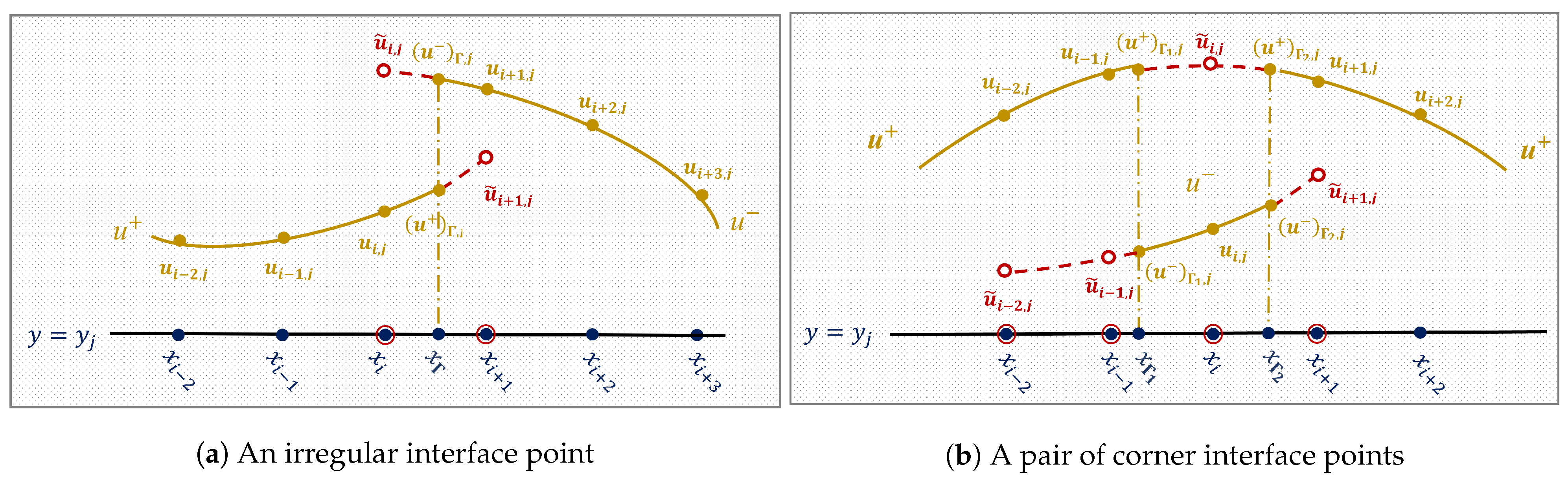
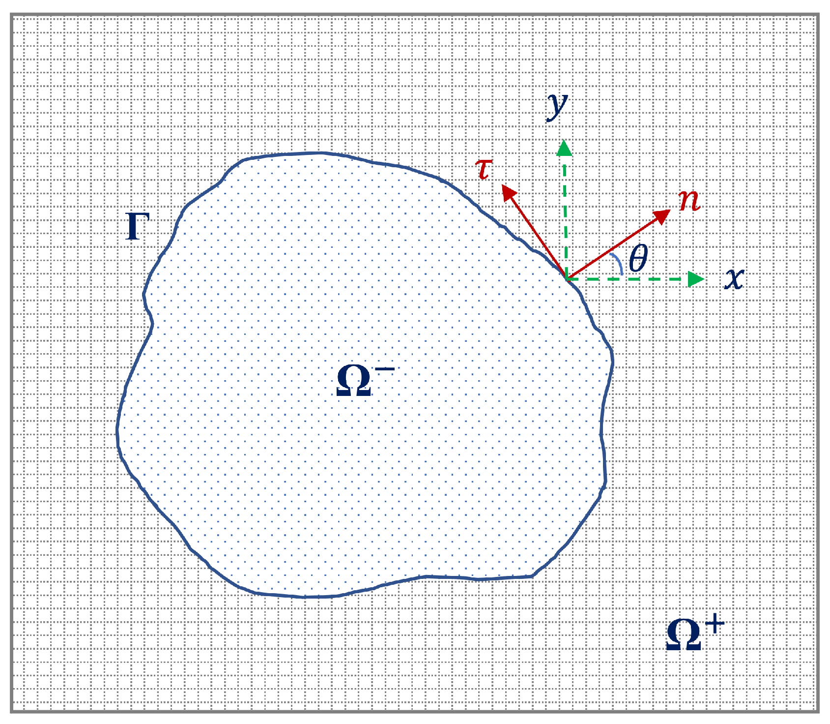
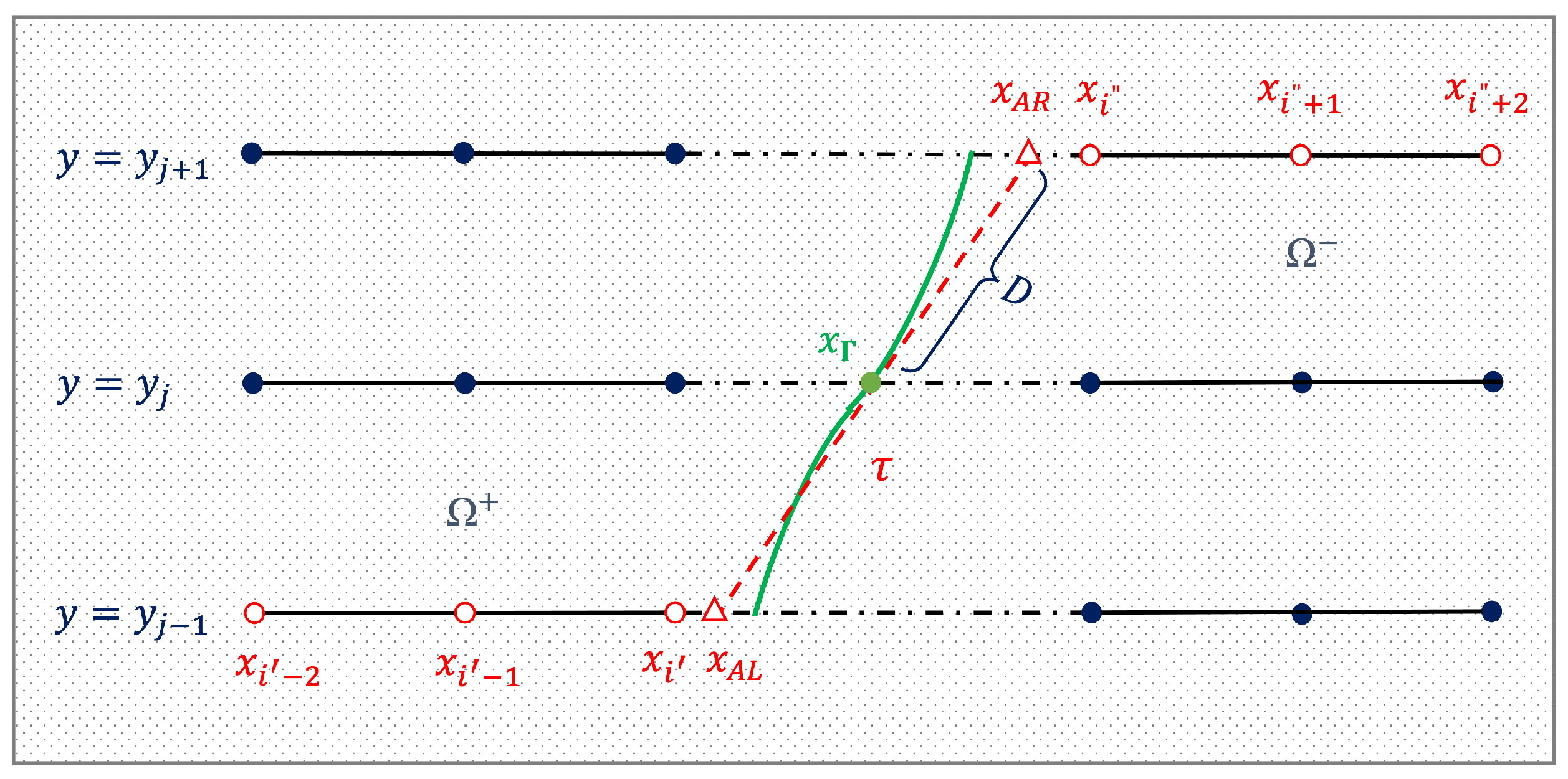
are obtained using the exact solution (31). The source term $f(x,y)$ can be obtained by using the governing equation. Consider an interface point with the normal direction being $\overrightarrow{n}=(cos\theta ,sin\theta )$, where $\theta$ is the angle between the normal direction and the positive x direction. The jump conditions at this point can be calculated via Equation (31) and (37)

$$\begin{array}{ccc}\hfill \left[u\right]& =& (cos(2x)sin(2y)-sin(2x)cos(2y\left)\right)cos\left(t\right),\hfill \end{array}$$

(34)

$$\begin{array}{ccc}\hfill \left[\alpha u_n\right]& =& 2(sin\left(2x\right)sin\left(2y\right)({\beta }^{-}sin\left(\theta \right)-{\beta }^{+}cos\left(\theta \right))\hfill \\ & & +cos\left(2x\right)cos\left(2y\right)({\beta }^{+}sin\left(\theta \right)-{\beta }^{-}cos\left(\theta \right)))cos\left(t\right).\hfill \end{array}$$

(35)

where ${\beta }^{+}$ and ${\beta }^{-}$ are the limiting values of $\beta$ at this interface point. We note that both jump conditions are temporally and spatially dependent to represent the most general jump conditions imposed on the interface $\mathsf{\Gamma }$.

All numerical experiments were conducted on a high-performance computing (HPC) cluster equipped with 24 Intel(R) Xeon(R) CPU E5-2670 v3 @ 2.30GHz and 128 GB RAM. Numerical $L^{\infty }$ and $L^2$ errors, which are defined as

$$\begin{array}{c}{\displaystyle L^{\infty }:=\underset{0\le i\le N_x,0\le j\le N_y}{max}|u(t_n,x_i,y_j)-U_{i,j}^n|,}\hfill \\ {\displaystyle L^2:=\sum _{0\le i\le N_x,0\le j\le N_y}\frac{{(u(t_n,x_i,y_j)-u_{i,j}^n)}^2}{N_x{N}_y}}\hfill \end{array}$$

(36)

at various final times are reported for all examples in order to quantitatively measure the accuracy of the proposed methods. The execution time, known as the wall clock time, taken from the start of the scientific program, FDIPS, to the end was used to demonstrate the efficiency of the proposed methods.

3.1. Efficiency Demonstration

The efficiency of ADI time stepping schemes is demonstrated first in this subsection. To this end, a simple “squircle” interface with a parametric form

$$\gamma \left(\rho \right)=0.5+0.05sin\left(4\rho \right)$$

for $0\le \rho \le 2\pi$ is considered. For simplicity, a piecewise constant $\beta$, which is defined as $\beta =1$ in ${\mathsf{\Omega }}^{-}$ and $\beta =10$ in ${\mathsf{\Omega }}^{+}$, is adopted, and the analytical solution is given by Equation (31). The interface and solution are shown in Figure 4a. The ADID1 method is employed for time advancing and compared to its analog, the implicit Euler (IE) method, to solve the 2D parabolic interface problem when both time stepping methods are coupled with the MIB method from an initial time $t_0=0$ to a final time $T=1$ with a fixed time step $\Delta t=1.0\times {10}^{-5}$.Various numbers of grid sizes with $N_x(=N_y)$ ranging from 41 to 201 are used. The obtained $L^2$ and $L^{\infty }$ errors are shown in Figure 4b. One can see the both MIB-IE and MIB-ADID1 schemes yield similar errors and have the same convergence pattern. The ADI errors are consistently smaller and such differences are believed to be caused by a higher perturbation term $\beta \Delta t^2{\delta }_{xx}{\delta }_{yy}u$ as indicated in [10]. The wall clock time of the two methods is demonstrated in Figure 4c. It is obvious that MIB-ADID1 is more efficient, for instance, about four times faster than MIB-IE at $N_x=201$. This is because a large linear system has to be solved by an iterative algorithm in each time step for the MIB-IE scheme. Provided the fact that both ADID1 and IE produce close errors while ADID1 is more efficient in time advancing, it is natural to choose ADI-type time stepping schemes in the proposed methods, which are utilized to solve the following 2D examples.

3.2. Variable Coefficient Examples

In all examples of this subsection, the diffusion coefficient $\beta$ is defined as a piecewise smooth function

$$\begin{array}{c}\hfill \beta (x,y)=\left\{\begin{array}{cc}{e}^{-(x^2+y^2)}\hfill & \mathrm{in}{\mathsf{\Omega }}^{-}\hfill \\ e^{x^2+y^2}\hfill & \mathrm{in}{\mathsf{\Omega }}^{+}\hfill \end{array}\right.\end{array}$$

(37)

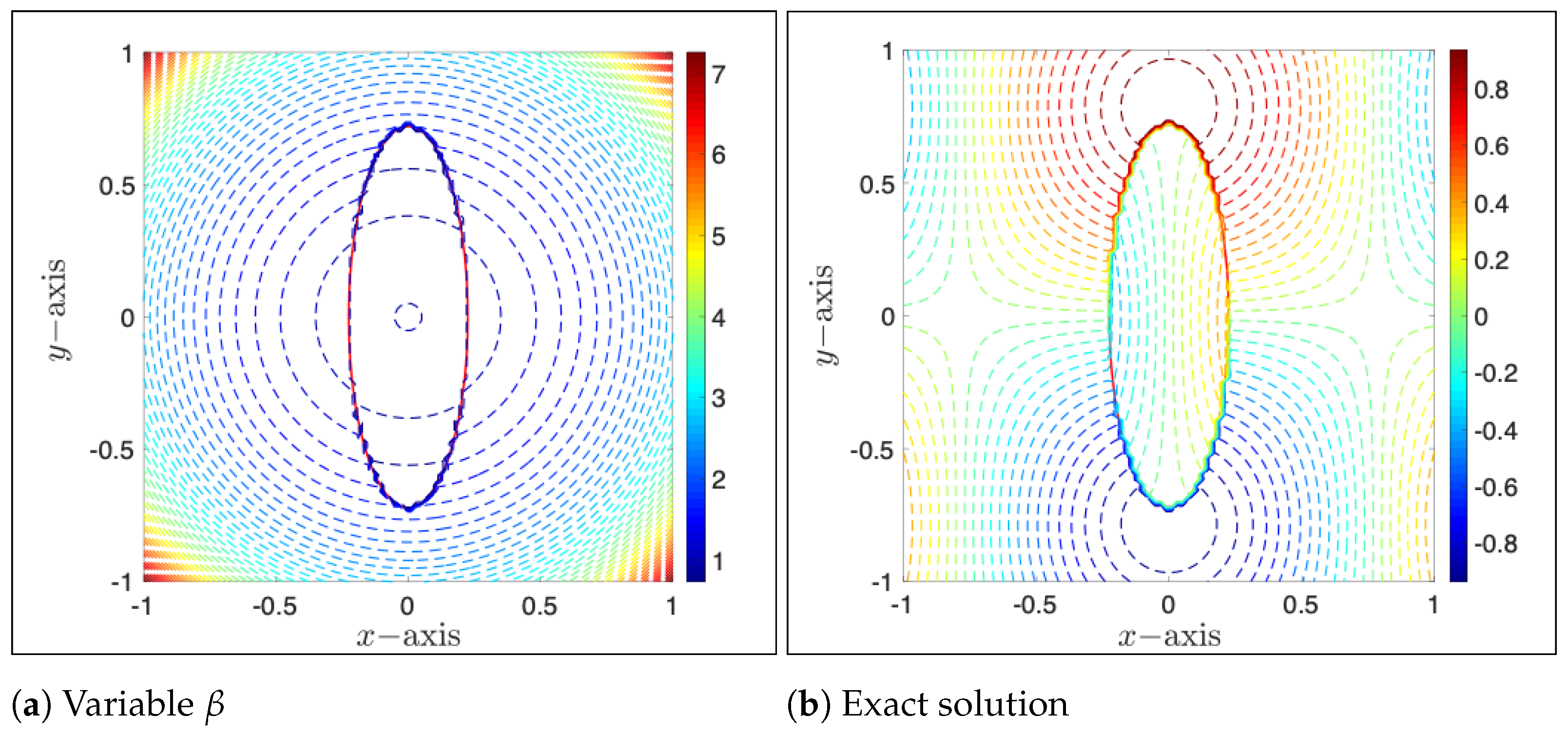
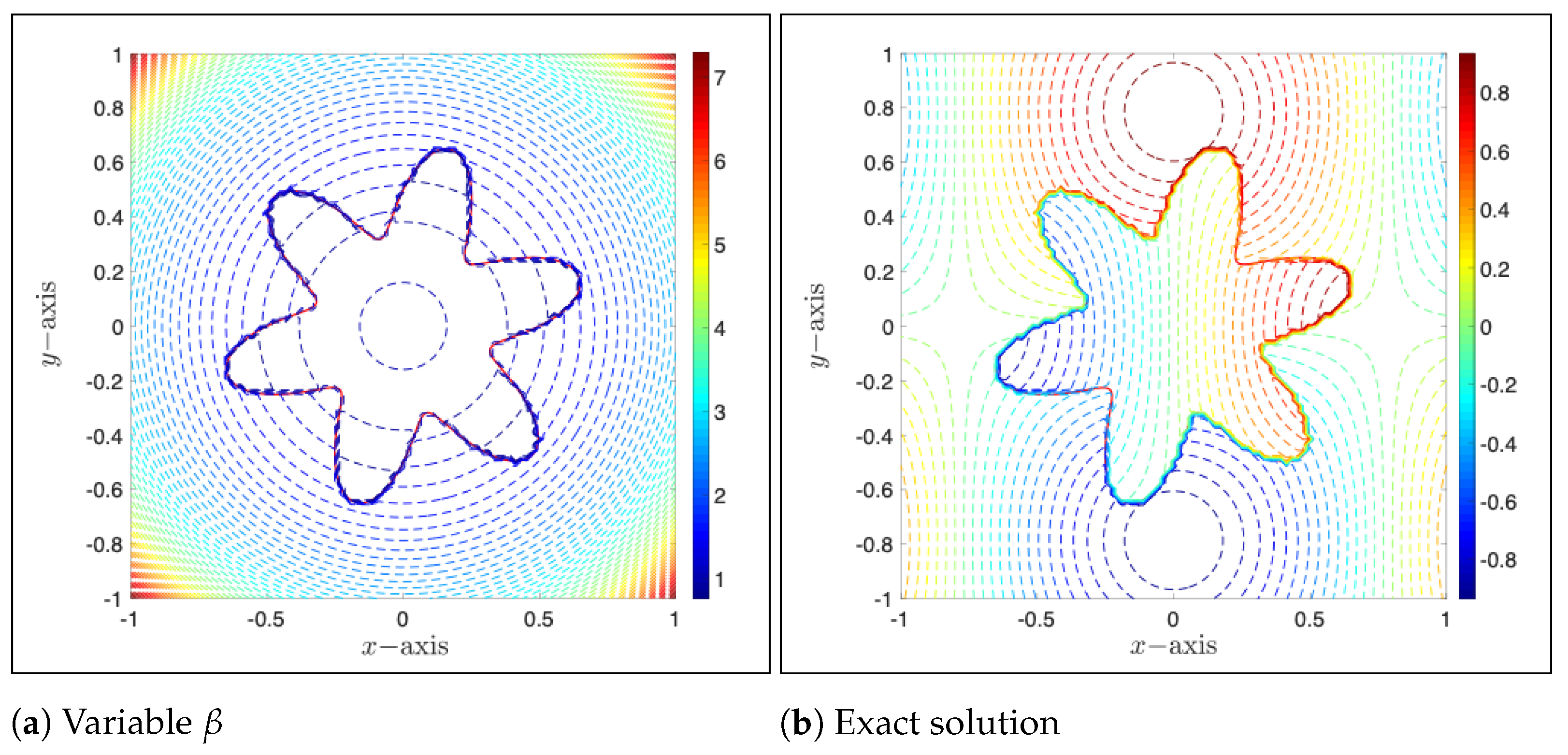
Example 1.

In the first example, the interface Γ is an ellipse constructed by the level set function

$$\phi (x,y)=0.9-\sqrt{{\left(4.0x\right)}^2+{\left(1.5y\right)}^2}.$$

(38)

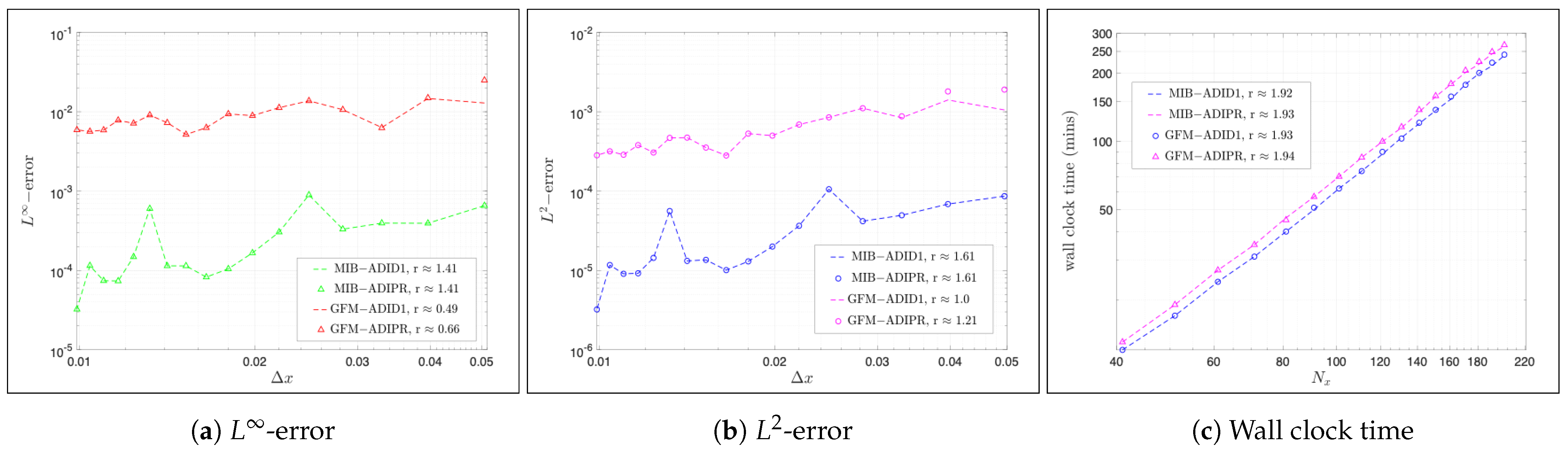
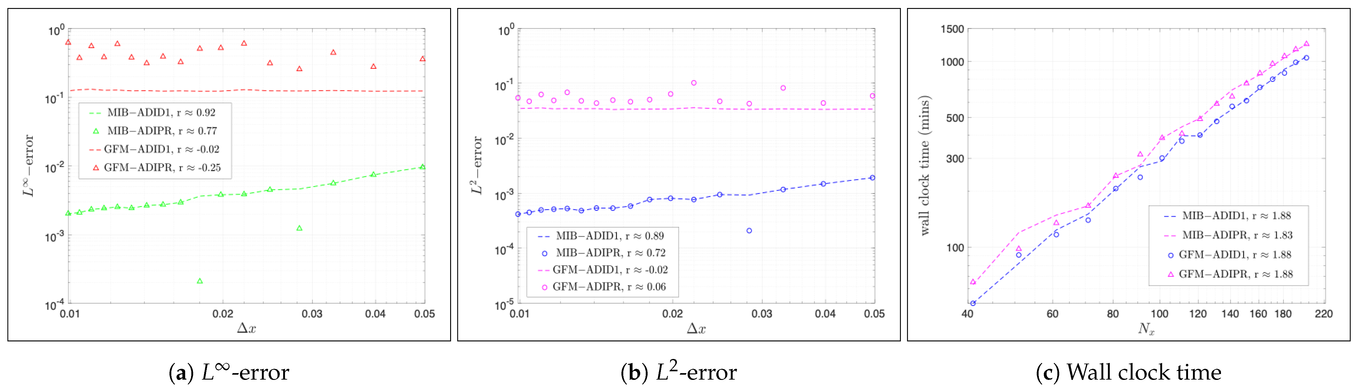
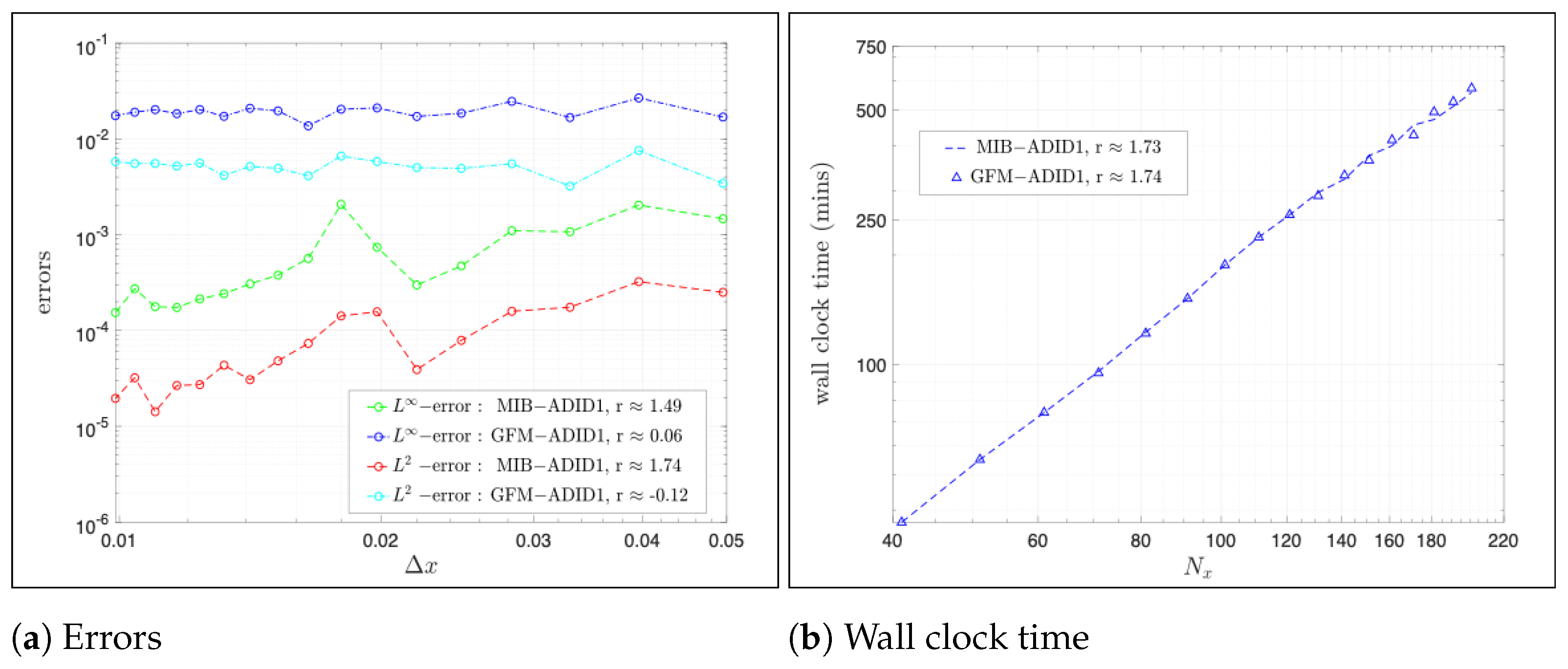
Contour plots of the diffusion coefficient (37) and exact solution (31) over the whole domain Ω are shown in Figure 5. Discontinuity on the interface can be easily observed in both graphs.

Spatial convergence tests are conducted first to compare the performance of the two spatial discretization methods, MIB and GFM. To this end, the time step is fixed to be small, $\Delta t=1.0\times {10}^{-6}$, and $N_x(=N_y)$ varies from 41 to 201 with an increment of 10 for all four proposed numerical methods. Log–log plots of $L^{\infty }$ and $L^2$ errors at the final time $T=1$ are shown in Figure 6a,b, respectively. All four methods are found to converge and be capable of achieving reasonable accuracy. The two MIB-involved methods achieve similar accuracy in the range of $(1.0\times {10}^{-5},1.0\times {10}^{-3})$ for $L^{\infty }$ error and $(1.0\times {10}^{-6},1.0\times {10}^{-4})$ for $L^2$ error, respectively, which are about two-magnitude smaller than those achieved by the two GFM-involved methods in all tested cases. Moreover, convergent rates are calculated using MATLAB subroutine polyfit and reported in Figure 6a,b as well. It can be seen that for the $L^2$ errors, the rates of the MIB schemes are about 1.6, while those of the GFM schemes are essentially 1. We believe the difference is caused by the hypothesis made in the GFM—it not only lowers the accuracy but also degrades the convergence rate. By considering a fixed number of time steps, wall clock times against $N_x$ are presented using log–log plot in Figure 6c. Execution times of all four methods are found to be almost same and increase at a similar rate slightly less than two. It is thus our belief that all methods are essentially equivalently efficient and they are all fast $O\left(N^2\right)$-methods where N stands for the number of grids per direction.

We next test the stability of four methods. To this end, we will consider various $\Delta t$ values, and for each $\Delta t$, a very long time integration is conducted with the number of time steps being 10,000. By considering two spatial meshes with $N_x=81$ and $N_x=281$, stability results are presented in

Table 1. Stability tests of Example 1.

	${\mathit{N}}_{\mathit{x}}(={\mathit{N}}_{\mathit{y}})=81$
$\mathit{T}(={\mathit{10}}^{\mathit{4}}·\Delta \mathit{t})$	MIB-ADID1		MIB-ADIPR		GFM-ADID1		GFM-ADIPR
	${\mathit{L}}^{\infty }$	${\mathit{L}}^{\mathit{2}}$	${\mathit{L}}^{\infty }$	${\mathit{L}}^{\mathit{2}}$	${\mathit{L}}^{\infty }$	${\mathit{L}}^{\mathit{2}}$	${\mathit{L}}^{\infty }$	${\mathit{L}}^{\mathit{2}}$
$1.00\times {10}^2$	$1.37\times {10}^{-2}$	$7.27\times {10}^{-4}$	$3.47\times {10}^{-2}$	$3.41\times {10}^{-3}$	$2.27\times {10}^{-2}$	$1.22\times {10}^{-3}$	$2.34\times {10}^{-2}$	$2.29\times {10}^{-3}$
$1.00\times {10}^1$	$1.33\times {10}^{-3}$	$1.51\times {10}^{-4}$	$1.43\times {10}^{-3}$	$1.49\times {10}^{-4}$	$2.10\times {10}^{-2}$	$1.26\times {10}^{-3}$	$2.11\times {10}^{-2}$	$1.26\times {10}^{-3}$
$1.00\times {10}^0$	$8.92\times {10}^{-4}$	$1.06\times {10}^{-4}$	$8.94\times {10}^{-4}$	$1.05\times {10}^{-4}$	$1.37\times {10}^{-2}$	$8.50\times {10}^{-4}$	$1.37\times {10}^{-2}$	$8.50\times {10}^{-4}$
$1.00\times {10}^{-1}$	$1.43\times {10}^{-3}$	$1.23\times {10}^{-4}$	$1.43\times {10}^{-3}$	$1.23\times {10}^{-4}$	$2.39\times {10}^{-2}$	$1.23\times {10}^{-3}$	$2.39\times {10}^{-2}$	$1.23\times {10}^{-3}$
	${\mathit{N}}_{\mathit{x}}(={\mathit{N}}_{\mathit{y}})=\mathit{281}$
$\mathit{T}(={\mathit{10}}^{\mathit{4}}·\Delta \mathit{t})$	MIB-ADID1		MIB-ADIPR		GFM-ADID1		GFM-ADIPR
	${\mathit{L}}^{\infty }$	${\mathit{L}}^{\mathit{2}}$	${\mathit{L}}^{\infty }$	${\mathit{L}}^{\mathit{2}}$	${\mathit{L}}^{\infty }$	${\mathit{L}}^{\mathit{2}}$	${\mathit{L}}^{\infty }$	${\mathit{L}}^{\mathit{2}}$
$1.00\times {10}^2$	$8.64\times {10}^{-2}$	$2.52\times {10}^{-3}$	-	-	$1.36\times {10}^{-2}$	$3.81\times {10}^{-4}$	$3.58\times {10}^{-1}$	$1.81\times {10}^{-2}$
$1.00\times {10}^1$	$1.05\times {10}^{-3}$	$2.34\times {10}^{-5}$	$7.11\times {10}^{-3}$	$8.60\times {10}^{-4}$	$7.78\times {10}^{-3}$	$3.87\times {10}^{-4}$	$7.86\times {10}^{-3}$	$4.46\times {10}^{-4}$
$1.00\times {10}^0$	$2.64\times {10}^{-5}$	$1.70\times {10}^{-6}$	$1.16\times {10}^{-4}$	$1.49\times {10}^{-5}$	$5.09\times {10}^{-3}$	$2.69\times {10}^{-4}$	$5.09\times {10}^{-3}$	$2.69\times {10}^{-4}$
$1.00\times {10}^{-1}$	$4.57\times {10}^{-5}$	$2.87\times {10}^{-6}$	$4.56\times {10}^{-5}$	$2.84\times {10}^{-6}$	$8.90\times {10}^{-3}$	$3.20\times {10}^{-4}$	$8.90\times {10}^{-3}$	$3.20\times {10}^{-4}$

. All computations are found to be stable, except for one case of the MIB-ADIPR method with $N_x=281$ and $\Delta t=1.0\times {10}^{-2}$. The errors for this unstable case are skipped and marked with dash signs in Table 1. The present study suggests that the MIB-ADIPR is the least stable method among the four methods. Moreover, the results shown in Table 1 also indicate that the two MIB-involved methods are usually more accurate than two GFM schemes.

It is meaningful to numerically study the condition of $\Delta t$ in terms of h when the MIB-ADIPR converges. To this end, $N_x=181,281,381,481$ are selected and for each $N_x$ value, and the largest stable $\Delta t$ value is searched via the bisection method. The least square fitting of the resulting $\Delta t$’s and h’s lead to a numerical stability condition for the MIB-ADIPR scheme, i.e., $\Delta t\le 11.7h^{1.88}$.

Temporal convergence is studied next. In this set of tests, the spatial mesh is fixed to be reasonably large, $N_x=N_y=391$, while the time step varies from $\Delta t=1.0\times {10}^{-2}$ down to $\Delta t=1.0\times {10}^{-4}$. The resulting $L^{\infty }$- and $L^2$- errors at the final time $T=1$ are reported in

Table 2. Temporal convergence tests of Example 1.

	MIB-ADID1				GFM-ADID1
$\Delta \mathit{t}$	${\mathit{L}}^{\infty }$		${\mathit{L}}^{\mathit{2}}$		${\mathit{L}}^{\infty }$		${\mathit{L}}^{\mathit{2}}$
	Error	Rate	Error	Rate	Error	Rate	Error	Rate
$1.00\times {10}^{-1}$	$9.35\times {10}^{-1}$	-	$7.11\times {10}^{-2}$	-	$5.65\times {10}^{-2}$	-	$1.35\times {10}^{-2}$	-
$5.00\times {10}^{-2}$	$5.52\times {10}^{-1}$	0.76	$2.70\times {10}^{-2}$	1.40	$3.36\times {10}^{-2}$	0.75	$4.09\times {10}^{-3}$	1.72
$1.00\times {10}^{-2}$	$1.10\times {10}^{-1}$	1.00	$3.17\times {10}^{-3}$	1.33	$6.14\times {10}^{-3}$	1.06	$4.18\times {10}^{-4}$	1.42
$5.00\times {10}^{-3}$	$5.10\times {10}^{-2}$	1.11	$1.06\times {10}^{-3}$	1.58	$4.73\times {10}^{-3}$	0.38	$2.82\times {10}^{-4}$	0.57
$1.00\times {10}^{-3}$	$7.28\times {10}^{-3}$	1.21	$3.97\times {10}^{-4}$	0.61	$4.73\times {10}^{-3}$	0.00	$2.06\times {10}^{-4}$	0.20
$5.00\times {10}^{-4}$	$1.94\times {10}^{-3}$	1.91	$1.11\times {10}^{-4}$	1.84	$4.81\times {10}^{-3}$	−0.24	$2.04\times {10}^{-4}$	0.01
$1.00\times {10}^{-4}$	$8.14\times {10}^{-5}$	1.97	$4.32\times {10}^{-6}$	2.02	$4.83\times {10}^{-3}$	0.00	$2.04\times {10}^{-4}$	0.00
	MIB-ADIPR				GFM-ADIPR
$\Delta \mathit{t}$	${\mathit{L}}^{\infty }$		${\mathit{L}}^{\mathit{2}}$		${\mathit{L}}^{\infty }$		${\mathit{L}}^{\mathit{2}}$
	Error	Rate	Error	Rate	Error	Rate	Error	Rate
$1.00\times {10}^{-1}$	-	-	-	-	$5.65\times {10}^{-2}$	-	$1.35\times {10}^{-2}$	-
$5.00\times {10}^{-2}$	-	-	-	-	$3.36\times {10}^{-2}$	0.75	$4.09\times {10}^{-3}$	1.72
$1.00\times {10}^{-2}$	-	-	-	-	$6.14\times {10}^{-3}$	1.06	$4.18\times {10}^{-4}$	1.42
$5.00\times {10}^{-3}$	$5.17\times {10}^{-1}$	-	$6.61\times {10}^{-2}$	-	$4.73\times {10}^{-3}$	0.38	$2.82\times {10}^{-4}$	0.57
$1.00\times {10}^{-3}$	$2.74\times {10}^{-2}$	1.83	$4.02\times {10}^{-3}$	1.74	$4.73\times {10}^{-3}$	0.00	$2.06\times {10}^{-4}$	0.20
$5.00\times {10}^{-4}$	$6.90\times {10}^{-3}$	1.99	$1.01\times {10}^{-3}$	1.99	$4.81\times {10}^{-3}$	−0.02	$2.04\times {10}^{-4}$	0.02
$1.00\times {10}^{-4}$	$2.80\times {10}^{-4}$	1.99	$4.16\times {10}^{-5}$	1.98	$4.83\times {10}^{-3}$	0.00	$2.04\times {10}^{-4}$	0.00

. Corresponding convergent rates are calculated by errors obtained at two consecutive tested time steps in Table 2.

A few important observations can be made on the results obtained in the temporal convergence tests. First, several entries are skipped in Table 2, because the MIB-ADIPR is unstable when $\Delta t\ge 1.0\times {10}^{-2}$. We note that the errors of unstable cases are much less than those in Table 1 in terms of magnitude. This is because the stopping time is fixed to be $T=1$ in the present study. Thus, the number of time steps is actually quite small for large $\Delta t$ values. Consequently, the error accumulation is not significant. On the other hand, all other three methods produce reasonably small errors and are believed to converge in all tested cases. Secondly, the convergence rates of the two MIB-involved methods are mostly within the range between one and two as expected. For the MIB-ADID1, the temporal convergence rate is about one initially but becomes close to two as $\Delta t$ is small enough. This is believed to be rooted in how the jump conditions are treated in the MIB method, i.e., tangential derivatives $u_{\tau }^{+}$ and $u_{\tau }^{-}$ at the next time step are approximated by their values at the current time step. The order of such approximation is $O(\Delta t)$, which significantly affects the temporal precision when $\Delta t$ is large. When $\Delta t$ is small enough, such approximation becomes negligible so that the temporal convergence is dominated by the ADI scheme itself. Thus the MIB-ADID1 method attains a second order temporal convergence when $\Delta t<1.0\times {10}^{-3}$. For the MIB-ADIPR method, once it is stable, its temporal convergence rate is about two, as shown in Table 2. However, the rates obtained by MIB-ADIPR are not seen to be significantly higher than those obtained by MIB-ADID1. Thirdly, the temporal rates of two GFM methods are about one initially but quickly drop to zero as $\Delta t$ becomes smaller. This means that the GFM spatial discretization invokes a quite large error, which finally dominates the computation. The refinement in time does not reduce the total error any further so that the temporal order becomes zero. In comparing with two GFM schemes, the two MIB-involved methods produce relatively larger errors when $\Delta t\ge 1.0\times {10}^{-3}$, but far fewer errors when $\Delta t<1.0\times {10}^{-3}$. A similar trend was observed when the diffusion coefficient is piecewise constant and is reported in Reference [15].

Results obtained in this example suggest that all four methods are able to produce satisfying numerical solutions when the step size is small. However, the MIB-ADID1 method is by far our most favorable method considering it is the most accurate and stable method. The geometric shape of the interface used in this example is rather simple, and we thereby continue to test the four methods in the next example with a more complicated interface.

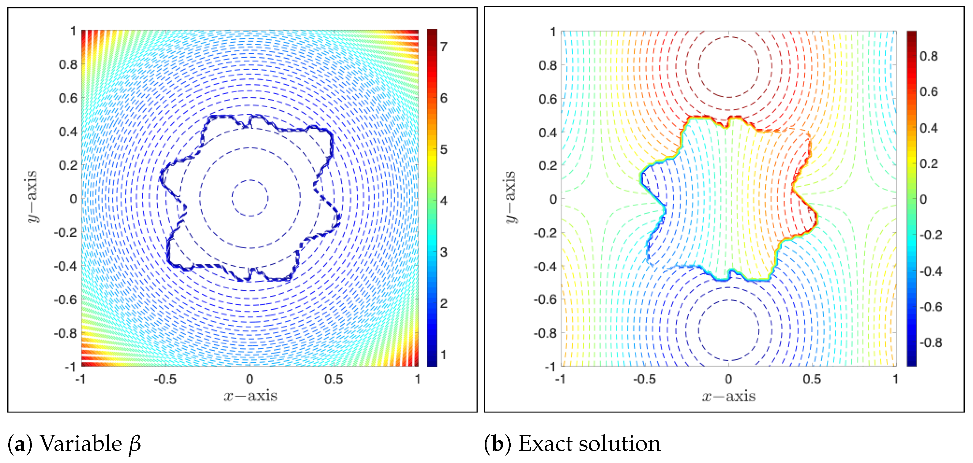
Example 2.

In the second example, the interface Γ is similar to that shown in the work [35]. The level set function is given by

$$\phi (x,y)=\sqrt{x^2+y^2}-r_0\left(1+\sum _{k=1}^3{\beta }_{k}cos\left(n_k\left(arctan\left(\frac{y}{x}\right)-{\theta }_k\right)\right)\right),$$

(39)

with parameters

$$r_0=0.483,\left(\begin{array}{c}{n}_1\\ {\beta }_1\\ {\theta }_1\end{array}\right)=\left(\begin{array}{c}3\\ 0.1\\ 0.5\end{array}\right),\left(\begin{array}{c}{n}_2\\ {\beta }_2\\ {\theta }_2\end{array}\right)=\left(\begin{array}{c}4\\ -0.1\\ 1.8\end{array}\right),and\left(\begin{array}{c}{n}_3\\ {\beta }_3\\ {\theta }_3\end{array}\right)=\left(\begin{array}{c}7\\ 0.15\\ 4.5\end{array}\right).$$

Contour plots of the diffusion coefficient and exact solution are shown in Figure 7. It is obvious that the shape of the interface in Example 2 is much more complex than that in Example 1. We want to see how the geometry of the interface impacts the proposed methods. Results obtained in spatial convergence, stability tests, and temporal convergence using the same numerical setup as that in Example 1 are shown in Figure 8,

Table 3. Stability tests of Example 2.

	${\mathit{N}}_{\mathit{x}}(={\mathit{N}}_{\mathit{y}})=81$
$\mathit{T}(={\mathit{10}}^{\mathit{4}}·\Delta \mathit{t})$	MIB-ADID1		MIB-ADIPR		GFM-ADID1		GFM-ADIPR
	${\mathit{L}}^{\infty }$	${\mathit{L}}^{\mathit{2}}$	${\mathit{L}}^{\infty }$	${\mathit{L}}^{\mathit{2}}$	${\mathit{L}}^{\infty }$	${\mathit{L}}^{\mathit{2}}$	${\mathit{L}}^{\infty }$	${\mathit{L}}^{\mathit{2}}$
$1.00\times {10}^2$	$1.52\times {10}^{-2}$	$1.24\times {10}^{-3}$	$2.40\times {10}^{-1}$	$1.28\times {10}^{-2}$	$8.05\times {10}^{-2}$	$1.90\times {10}^{-2}$	$9.23\times {10}^{-2}$	$1.79\times {10}^{-2}$
$1.00\times {10}^1$	$1.51\times {10}^{-3}$	$2.68\times {10}^{-4}$	$2.36\times {10}^{-3}$	$3.26\times {10}^{-4}$	$8.20\times {10}^{-2}$	$1.98\times {10}^{-2}$	$8.18\times {10}^{-2}$	$1.97\times {10}^{-2}$
$1.00\times {10}^0$	$1.14\times {10}^{-3}$	$2.08\times {10}^{-4}$	$1.16\times {10}^{-3}$	$2.13\times {10}^{-4}$	$5.45\times {10}^{-2}$	$1.34\times {10}^{-2}$	$5.43\times {10}^{-2}$	$1.33\times {10}^{-2}$
$1.00\times {10}^{-1}$	$2.00\times {10}^{-3}$	$3.34\times {10}^{-4}$	$2.00\times {10}^{-3}$	$3.34\times {10}^{-4}$	$8.53\times {10}^{-2}$	$1.89\times {10}^{-2}$	$8.47\times {10}^{-2}$	$1.88\times {10}^{-2}$
	${\mathit{N}}_{\mathit{x}}(={\mathit{N}}_{\mathit{y}})=\mathit{281}$
$\mathit{T}(={\mathit{10}}^{\mathit{4}}·\Delta \mathit{t})$	MIB-ADID1		MIB-ADIPR		GFM-ADID1		GFM-ADIPR
	${\mathit{L}}^{\infty }$	${\mathit{L}}^{\mathit{2}}$	${\mathit{L}}^{\infty }$	${\mathit{L}}^{\mathit{2}}$	${\mathit{L}}^{\infty }$	${\mathit{L}}^{\mathit{2}}$	${\mathit{L}}^{\infty }$	${\mathit{L}}^{\mathit{2}}$
$1.00\times {10}^2$	$1.32\times {10}^{-1}$	$5.98\times {10}^{-3}$	-	-	$9.17\times {10}^{-2}$	$1.98\times {10}^{-2}$	-	-
$1.00\times {10}^1$	$2.49\times {10}^{-3}$	$1.40\times {10}^{-4}$	$2.72\times {10}^{-2}$	$1.98\times {10}^{-3}$	$8.74\times {10}^{-2}$	$2.05\times {10}^{-2}$	$8.85\times {10}^{-2}$	$2.10\times {10}^{-2}$
$1.00\times {10}^0$	$2.32\times {10}^{-4}$	$4.22\times {10}^{-5}$	$3.99\times {10}^{-4}$	$6.45\times {10}^{-5}$	$5.83\times {10}^{-2}$	$1.39\times {10}^{-2}$	$5.83\times {10}^{-2}$	$1.39\times {10}^{-2}$
$1.00\times {10}^{-1}$	$6.16\times {10}^{-4}$	$1.05\times {10}^{-4}$	$6.17\times {10}^{-4}$	$1.05\times {10}^{-4}$	$8.89\times {10}^{-2}$	$1.98\times {10}^{-2}$	$8.89\times {10}^{-2}$	$1.98\times {10}^{-2}$

and

Table 4. Temporal convergence tests of Example 2.

	MIB-ADID1				GFM-ADID1
$\Delta \mathit{t}$	${\mathit{L}}^{\infty }$		${\mathit{L}}^{\mathit{2}}$		${\mathit{L}}^{\infty }$		${\mathit{L}}^{\mathit{2}}$
	Error	Rate	Error	Rate	Error	Rate	Error	Rate
$1.00\times {10}^{-1}$	$1.24\times {10}^0$	-	$1.33\times {10}^{-1}$	-	$7.02\times {10}^{-2}$	-	$1.53\times {10}^{-2}$	-
$5.00\times {10}^{-2}$	$6.48\times {10}^{-1}$	0.94	$4.95\times {10}^{-2}$	1.42	$6.12\times {10}^{-2}$	0.20	$1.28\times {10}^{-2}$	0.25
$1.00\times {10}^{-2}$	$1.35\times {10}^{-1}$	0.97	$5.85\times {10}^{-3}$	1.33	$5.36\times {10}^{-2}$	0.08	$1.34\times {10}^{-2}$	−0.03
$5.00\times {10}^{-3}$	$6.60\times {10}^{-2}$	1.03	$2.94\times {10}^{-3}$	1.00	$5.43\times {10}^{-2}$	−0.02	$1.34\times {10}^{-2}$	−0.03
$1.00\times {10}^{-3}$	$5.65\times {10}^{-3}$	1.53	$4.99\times {10}^{-4}$	1.10	$5.60\times {10}^{-2}$	−0.02	$1.34\times {10}^{-2}$	−0.01
$5.00\times {10}^{-4}$	$1.55\times {10}^{-3}$	1.87	$1.42\times {10}^{-4}$	1.81	$5.61\times {10}^{-2}$	−0.00	$1.34\times {10}^{-2}$	0.00
$1.00\times {10}^{-4}$	$1.29\times {10}^{-4}$	1.54	$2.16\times {10}^{-5}$	1.17	$5.62\times {10}^{-2}$	0.00	$1.34\times {10}^{-2}$	0.00
	MIB-ADIPR				GFM-ADIPR
$\Delta \mathit{t}$	${\mathit{L}}^{\infty }$		${\mathit{L}}^{\mathit{2}}$		${\mathit{L}}^{\infty }$		${\mathit{L}}^{\mathit{2}}$
	Error	Rate	Error	Rate	Error	Rate	Error	Rate
$1.00\times {10}^{-1}$	-	-	-	-	-	-	-	-
$5.00\times {10}^{-2}$	-	-	-	-	-	-	-	-
$1.00\times {10}^{-2}$	-	-	-	-	-	-	-	-
$5.00\times {10}^{-3}$	-	-	-	-	-	-	-	-
$1.00\times {10}^{-3}$	-	-	-	-	$2.74\times {10}^{-1}$	-	$2.40\times {10}^{-2}$	-
$5.00\times {10}^{-4}$	$3.18\times {10}^{-1}$	-	$1.27\times {10}^{-2}$	-	$1.73\times {10}^{-1}$	0.67	$1.57\times {10}^{-2}$	0.62
$1.00\times {10}^{-4}$	$1.29\times {10}^{-4}$	4.85	$2.16\times {10}^{-5}$	3.96	$7.61\times {10}^{-2}$	0.51	$1.42\times {10}^{-2}$	0.06

, respectively.

In Figure 8a,b, it is found that convergence rates obtained by the two MIB-involved methods are reduced to slightly less than one but are still much greater than the convergence rates obtained by the two GFM-involved methods. It is believed that the reduction of spatial convergence rates is due to the more complicated shape of the interface when jump conditions need to be taken care of at more irregular and corner pointers in the numerical procedure. Moreover, the corresponding wall clock time shown in Figure 8c is found to be higher than those obtained in Example 1 due to additional calculations required for additional jump conditions. However, the overall complexity is still $O\left(N^2\right)$ for both MIB and GFM methods.

The “negative” impact of the interface can also be observed in stability tests. In Table 3, both MIB-ADIPR and GFM-ADIPR become unstable for $N_x=281$ and $\Delta t=1.0\times {10}^{-2}$. It is definitely different from the results we obtained for solving problems with a piecewise constant diffusion coefficient in the work of [15], because all GFM-ADI methods are unconditionally stable in that context. For constant coefficient problems, the GFM finite difference matrices for ${\delta }_{xx}$ and ${\delta }_{yy}$ are symmetric. However, such symmetry is lost for the present variable coefficient problems. Consequently, the GFM-ADIPB becomes conditionally stable.

The temporal convergence tests are shown in Table 4. Both the MIB-ADID1 and GFM-ADID1 schemes produce larger errors than those obtained in Table 2, while the convergence patterns are very similar. Limited by the spatial accuracy of the GFM, the ADID1 stops to convergence as $\Delta t$ decreases. For the MIB-ADID1, the temporal order increases from one to two, as $\Delta t$ is decreasing. Moreover, more cases of the two ADIPR-involved methods are found to diverge, no matter which spatial discretization, either MIB or GFM, is used. As a matter of fact, it is hard to tell which spatial discretization method is better in terms of stability when solving problems with variable diffusion coefficient $\beta$.

Based on results presented in Examples 1 and 2, it is reasonable to believe that ADID1 is superior to ADIPR to be used for temporal discretization in terms of convergence and stability—both ADID1-involved methods converge in almost all tested cases, and the two ADIPR-involved methods converge only when the time step $\Delta t$ is small, and the results they obtain are not seen to be more accurate than those obtained by MIB-ADID1. Moreover, it seems that the MIB-ADID1 method, which maintains reasonable convergence rates in both spatial and temporal convergence tests, is the best method among all four proposed methods. In the examples that follow, we will just focus on testing the two ADID1-involved methods.

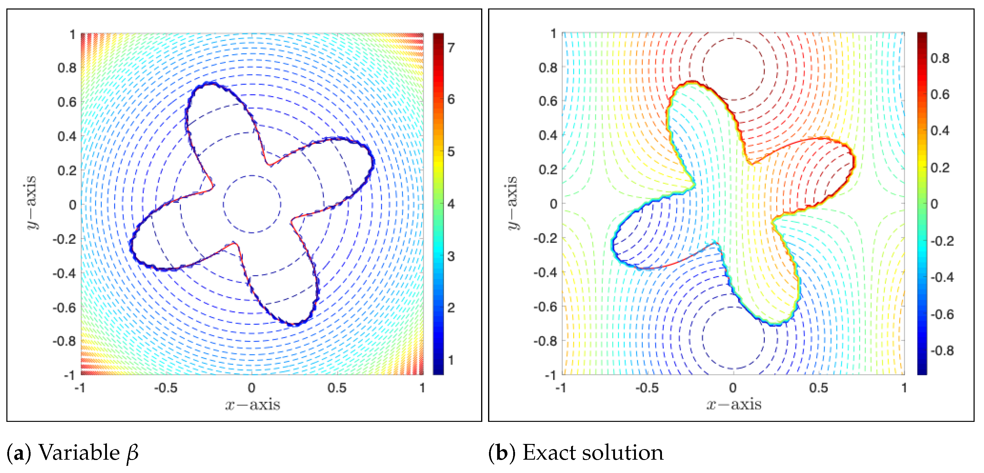
Example 3.

In our first example, a grid line cuts the interface at most at two irregular interface points due to the simplicity of the interface’s geometry. In the second example, a grid line can cut the interface more than twice, but corner interface points only occurred in a few cases. In the examples which follow, we would like to have both irregular and corner interface points occurring in many interface locations in order to earn more profound insight on how they are going to affect the proposed numerical methods. To this end, an interface constructed by a parametric function

$$\gamma \left(\eta \right)=0.5+bsin\left(k\eta \right),$$

(40)

is used in this and next example. Here $b>0$ governs the magnitude and curvature of the interface, $k>0$ is a positive integer determining the number of “heads” of the curve, and η is an angle in the range of $[0,2\pi ]$. By choosing parameters $(b,k)=(0.25,4)$, a four-head interface, together with imposed β and exact solution, is demonstrated in Figure 9. When compared to the interfaces used in Examples 1 and 2, this interface has sharper curvature at four corners so that corner interface points are encountered in almost all tested cases.

Using the same numerical setup, results obtained for spatial, temporal and stability tests on the two ADID1-invloved methods are reported in Figure 10,

Table 5. Stability tests of Example 3.

	${\mathit{N}}_{\mathit{x}}(={\mathit{N}}_{\mathit{y}})=81$				${\mathit{N}}_{\mathit{x}}(={\mathit{N}}_{\mathit{y}})=281$
$\mathit{T}(={\mathit{10}}^{\mathit{4}}·\Delta \mathit{t})$	MIB-ADID1		GFM-ADID1		MIB-ADID1		GFM-ADID1
	${\mathit{L}}^{\infty }$	${\mathit{L}}^{\mathit{2}}$	${\mathit{L}}^{\infty }$	${\mathit{L}}^{\mathit{2}}$	${\mathit{L}}^{\infty }$	${\mathit{L}}^{\mathit{2}}$	${\mathit{L}}^{\infty }$	${\mathit{L}}^{\mathit{2}}$
$1.00\times {10}^2$	$3.14\times {10}^{-2}$	$2.79\times {10}^{-3}$	$2.83\times {10}^{-2}$	$6.36\times {10}^{-3}$	$2.70\times {10}^{-1}$	$2.10\times {10}^{-2}$	$3.21\times {10}^{-2}$	$6.74\times {10}^{-3}$
$1.00\times {10}^1$	$5.58\times {10}^{-4}$	$9.52\times {10}^{-5}$	$2.73\times {10}^{-2}$	$6.99\times {10}^{-3}$	$5.59\times {10}^{-3}$	$4.99\times {10}^{-4}$	$2.73\times {10}^{-2}$	$8.04\times {10}^{-3}$
$1.00\times {10}^0$	$4.63\times {10}^{-4}$	$7.65\times {10}^{-5}$	$1.85\times {10}^{-2}$	$4.93\times {10}^{-3}$	$9.91\times {10}^{-5}$	$8.22\times {10}^{-6}$	$1.86\times {10}^{-2}$	$5.67\times {10}^{-3}$
$1.00\times {10}^{-1}$	$7.21\times {10}^{-4}$	$9.91\times {10}^{-5}$	$2.50\times {10}^{-2}$	$4.88\times {10}^{-3}$	$1.33\times {10}^{-4}$	$1.51\times {10}^{-5}$	$2.42\times {10}^{-2}$	$5.48\times {10}^{-3}$

and

Table 6. Temporal efficiency tests of Example 3.

	MIB-ADID1				GFM-ADID1
$\Delta \mathit{t}$	${\mathit{L}}^{\infty }$		${\mathit{L}}^{\mathit{2}}$		${\mathit{L}}^{\infty }$		${\mathit{L}}^{\mathit{2}}$
	Error	Rate	Error	Rate	Error	Rate	Error	Rate
$1.00\times {10}^{-1}$	$2.17\times {10}^0$	-	$1.96\times {10}^{-1}$	-	$6.74\times {10}^{-2}$	-	$1.43\times {10}^{-2}$	-
$5.00\times {10}^{-2}$	$1.25\times {10}^0$	0.80	$9.35\times {10}^{-2}$	1.06	$3.92\times {10}^{-2}$	0.78	$5.97\times {10}^{-3}$	1.27
$1.00\times {10}^{-2}$	$3.19\times {10}^{-1}$	0.85	$1.72\times {10}^{-2}$	1.05	$1.84\times {10}^{-2}$	0.47	$4.94\times {10}^{-3}$	0.12
$5.00\times {10}^{-3}$	$1.86\times {10}^{-1}$	0.78	$1.09\times {10}^{-2}$	0.66	$1.75\times {10}^{-2}$	0.07	$5.01\times {10}^{-3}$	−0.02
$1.00\times {10}^{-3}$	$2.51\times {10}^{-2}$	1.24	$2.11\times {10}^{-3}$	1.02	$1.69\times {10}^{-2}$	0.02	$4.98\times {10}^{-3}$	0.04
$5.00\times {10}^{-4}$	$6.65\times {10}^{-3}$	1.92	$5.68\times {10}^{-4}$	1.89	$1.69\times {10}^{-2}$	0.00	$4.98\times {10}^{-3}$	0.00
$1.00\times {10}^{-4}$	$2.78\times {10}^{-4}$	1.97	$2.30\times {10}^{-5}$	1.99	$1.69\times {10}^{-2}$	0.00	$4.98\times {10}^{-3}$	0.00

, respectively. No significant differences are observed in the results obtained in this example when compared to those obtained in the previous two examples. In fact, the rates obtained in spatial tests (Figure 10) and temporal tests (Table 6) are similar to those obtained in Examples 1 and 2, and no divergence is found in stability tests (Table 5). It suggests that the numerical treatments introduced in both MIB and GFM methods are equally accurate when dealing with the jumps imposed at irregular and corner interface points. Moreover, wall clock time shown in Figure 10b is between those shown in Figure 6c and Figure 8c, suggesting that the efficiency of both methods is not jeopardized significantly by the corner points either.

Example 4.

The results obtained in Example 3 have clearly demonstrated the robustness and efficiency of the two proposed methods when treating jump conditions at both irregular and corner interface points. In the last example, we continue to make the interface sharper with more interface points by choosing $(b,k)=(0.15,6)$ in Equation (40), resulting in a six-head interface with fast changing curvature shown in Figure 11. Similar numerical results are shown in Figure 12 and

Table 7. Stability tests of Example 4.

$\mathit{T}(={10}^4·\mathbf{\Delta }\mathit{t})$	${\mathit{N}}_{\mathit{x}}(={\mathit{N}}_{\mathit{y}})=81$				${\mathit{N}}_{\mathit{x}}(={\mathit{N}}_{\mathit{y}})=281$
	MIB-ADID1		GFM-ADID1		MIB-ADID1		GFM-ADID1
	${\mathit{L}}^{\infty }$	${\mathit{L}}^{\mathit{2}}$	${\mathit{L}}^{\infty }$	${\mathit{L}}^{\mathit{2}}$	${\mathit{L}}^{\infty }$	${\mathit{L}}^{\mathit{2}}$	${\mathit{L}}^{\infty }$	${\mathit{L}}^{\mathit{2}}$
$1.00\times {10}^2$	$2.02\times {10}^{-2}$	$2.07\times {10}^{-3}$	$1.92\times {10}^{-2}$	$3.73\times {10}^{-3}$	$2.32\times {10}^{-1}$	$1.81\times {10}^{-2}$	$1.59\times {10}^{-2}$	$2.52\times {10}^{-3}$
$1.00\times {10}^1$	$3.59\times {10}^{-4}$	$7.48\times {10}^{-5}$	$1.84\times {10}^{-2}$	$4.06\times {10}^{-3}$	$4.98\times {10}^{-3}$	$5.62\times {10}^{-4}$	$1.15\times {10}^{-2}$	$2.76\times {10}^{-3}$
$1.00\times {10}^0$	$2.76\times {10}^{-4}$	$5.66\times {10}^{-5}$	$1.24\times {10}^{-2}$	$2.83\times {10}^{-3}$	$8.46\times {10}^{-5}$	$6.57\times {10}^{-6}$	$7.78\times {10}^{-3}$	$1.93\times {10}^{-3}$
$1.00\times {10}^{-1}$	$4.79\times {10}^{-4}$	$8.63\times {10}^{-5}$	$1.78\times {10}^{-2}$	$3.17\times {10}^{-3}$	$9.96\times {10}^{-5}$	$1.79\times {10}^{-5}$	$1.10\times {10}^{-2}$	$2.01\times {10}^{-3}$

and

Table 8. Temporal efficiency tests of Example 4.

	MIB-ADID1				GFM-ADID1
$\Delta \mathit{t}$	${\mathit{L}}^{\infty }$		${\mathit{L}}^{\mathit{2}}$		${\mathit{L}}^{\infty }$		${\mathit{L}}^{\mathit{2}}$
	Error	Rate	Error	Rate	Error	Rate	Error	Rate
$1.00\times {10}^{-1}$	$1.44\times {10}^0$	-	$1.51\times {10}^{-1}$	-	$4.40\times {10}^{-2}$	-	$1.36\times {10}^{-2}$	-
$5.00\times {10}^{-2}$	$7.10\times {10}^{-1}$	1.02	$5.88\times {10}^{-2}$	1.36	$2.62\times {10}^{-2}$	0.75	$4.42\times {10}^{-3}$	1.62
$1.00\times {10}^{-2}$	$1.48\times {10}^{-1}$	0.98	$7.83\times {10}^{-3}$	1.25	$9.05\times {10}^{-3}$	0.66	$1.86\times {10}^{-3}$	0.54
$5.00\times {10}^{-3}$	$8.22\times {10}^{-2}$	0.85	$4.55\times {10}^{-3}$	0.78	$7.83\times {10}^{-3}$	0.21	$1.82\times {10}^{-3}$	0.03
$1.00\times {10}^{-3}$	$1.24\times {10}^{-2}$	1.18	$1.62\times {10}^{-3}$	0.64	$7.26\times {10}^{-3}$	0.05	$1.79\times {10}^{-3}$	0.01
$5.00\times {10}^{-4}$	$3.31\times {10}^{-3}$	1.90	$4.43\times {10}^{-4}$	1.87	$7.29\times {10}^{-3}$	0.00	$1.79\times {10}^{-3}$	0.00
$1.00\times {10}^{-4}$	$1.33\times {10}^{-4}$	2.00	$1.74\times {10}^{-5}$	2.01	$7.30\times {10}^{-3}$	0.00	$1.79\times {10}^{-3}$	0.00

. Once again, no significant differences are observed, and both methods well maintain their performance in previous examples as expected. In fact, the ADI-ADID1 attains the second order convergence in space for this variable coefficient example.

Provided the interface used in this example is the most general one reported in this work, one additional set of tests is conducted to study one more factor, the contrast of $\beta$’s values inside and outside the interface, which could also affect the convergence and stability of the methods. To this end, the diffusion coefficient $\beta$ in Equation (37) is redefined as

$$\begin{array}{c}\hfill \beta (x,y)=\left\{\begin{array}{cc}{e}^{-(x^2+y^2)}\hfill & \mathrm{in}{\mathsf{\Omega }}^{-}\hfill \\ r{e}^{x^2+y^2}\hfill & \mathrm{in}{\mathsf{\Omega }}^{+}\hfill \end{array}\right.\end{array}$$

(41)

with an additional ratio coefficient $r>0$ so that the contrast of $\beta$ values inside and outside the interface can be varied. Results obtained by varying the value of r from $r=1/320$ to $r=320$ are presented in

Table 9. $\beta$ tests of Example 4.

Ratio r	MIB-ADID1		GFM-ADID1		Ratio r	MIB-ADID1		GFM-ADID1
	${\mathit{L}}^{\infty }$	${\mathit{L}}^{\mathit{2}}$	${\mathit{L}}^{\infty }$	${\mathit{L}}^{\mathit{2}}$		${\mathit{L}}^{\infty }$	${\mathit{L}}^{\mathit{2}}$	${\mathit{L}}^{\infty }$	${\mathit{L}}^{\mathit{2}}$
$1/320$	$4.22\times {10}^{-1}$	$4.66\times {10}^{-2}$	$1.63\times {10}^{-2}$	$1.81\times {10}^{-3}$	1	$2.32\times {10}^{-1}$	$1.81\times {10}^{-2}$	$1.59\times {10}^{-2}$	$2.52\times {10}^{-3}$
$1/160$	$4.17\times {10}^{-1}$	$4.72\times {10}^{-2}$	$1.65\times {10}^{-2}$	$1.76\times {10}^{-3}$	10	$1.75\times {10}^0$	$1.85\times {10}^{-1}$	$3.44\times {10}^{-2}$	$2.43\times {10}^{-3}$
$1/80$	$4.03\times {10}^{-1}$	$4.63\times {10}^{-2}$	$1.67\times {10}^{-2}$	$1.83\times {10}^{-3}$	20	$2.57\times {10}^0$	$3.12\times {10}^{-1}$	$5.31\times {10}^{-2}$	$4.11\times {10}^{-3}$
$1/40$	$3.70\times {10}^{-1}$	$4.09\times {10}^{-2}$	$1.69\times {10}^{-2}$	$1.90\times {10}^{-3}$	40	-	-	$7.15\times {10}^{-2}$	$7.31\times {10}^{-3}$
$1/20$	$3.02\times {10}^{-1}$	$3.35\times {10}^{-2}$	$1.72\times {10}^{-2}$	$1.83\times {10}^{-3}$	80	-	-	$9.87\times {10}^{-2}$	$1.35\times {10}^{-2}$
$1/10$	$2.97\times {10}^{-1}$	$2.82\times {10}^{-2}$	$1.74\times {10}^{-2}$	$2.50\times {10}^{-3}$	160	-	-	$1.83\times {10}^{-1}$	$2.62\times {10}^{-2}$
					320	-	-	$3.54\times {10}^{-1}$	$5.23\times {10}^{-2}$

, with the other numerical parameters being fixed as: $N_x=281$, $\Delta t=1.0\times {10}^{-2}$, and $T={10}^4\ast \Delta t=1.0\times {10}^2$. One can see that both methods are stable and able to produce reasonable errors when the contrast ratio r is small, while MIB-ADID1 starts to become unstable and produce relatively large errors when r is large, i.e., $r>20$. On the other hand, GFM-ADID1 is still able to maintain its stability and produce reasonable errors even when the ratio r is as large as 320. Moreover, one may also notice that, in Table 9, errors obtained by GFM-ADID1 are smaller than those obtained by MIB-ADID1. Based on the results shown in Table 9, we conclude that GFM-ADID1 has a better chance to converge when the contrast of $\beta$’s values and time step $\Delta t$ are large, while MIB-ADID1 shall be better when small $\Delta t$ is utilized. This conclusion matches what we observed for piecewise constant $\beta$ in [15].

4. Conclusions

In this paper, two new alternating direction implicit (ADI) schemes are developed and compared for solving parabolic interface problems with variable coefficients. In order to enforce the 2D jump conditions in the dimension-by-dimension ADI computations, a tensor product decomposition shall be conducted to generate 1D jump conditions for correcting the finite difference discretization. To this end, the tangential jumps are estimated from the previous time step in the matched interface and boundary (MIB) scheme, while they are simply neglected in the ghost fluid method (GFM). The resulting MIB-ADI method is semi-implicit, while the GFM-ADI method is still fully implicit. Moreover, in addition to the Douglas ADI (ADID1) scheme, the Peaceman–Rachfor ADI (ADIPR) scheme is also employed to couple with both MIB and GFM methods. Various numerical tests are conducted to investigate the accuracy, efficiency, and stability of the proposed ADI methods. When the time step $\Delta t$ is small, all four ADI schemes can recover the accuracy reduction near interfaces, while maintaining the ADI efficiency.

A comparison of four ADI schemes for solving variable coefficient parabolic interface problems has been carried out and can be summarized as follows:

• Stability: Two ADIPR schemes are found to be unstable when $\Delta t$ is large, while most reported ADID1 results are stable. This is because the ADIPR scheme is constructed based on the Crank–Nicolson time integration, which is less stable than the implicit Euler time integration behind the ADID1 scheme. Although no instability is detected for the GFM-ADID1 scheme, both MIB-ADID1 and GFM-ADID1 methods are believed to be conditionally stable for variable coefficient heat equations with material interfaces. For the MIB-ADID1 scheme, this is due to its semi-implicit nature. The GFM-ADID1 method is known to be unconditionally stable for solving parabolic interface problems with a piecewise constant diffusion coefficient [15] because the GFM finite difference matrices for ${\delta }_{xx}$ and ${\delta }_{yy}$ are symmetric and diagonal dominate. However, such symmetry is lost for the present variable coefficient problems. As a consequence, the GFM-ADID1 could become conditionally stable. Based on the present result for the MIB-ADIPR, the stability condition of the proposed ADI methods shall take the general form $\Delta t\le C{h}^2$, where the constant C should depend on the ADID1 or ADIPR time integration, as well as the diffuse coefficient $\beta$. Although the stability condition has the same form as that of the explicit methods, the constant C is usually a quite large number in the ADID1 methods, so that when h is not too small, the computation is still stable for large $\Delta t$ values.
• Spatial accuracy: The GFM method can improve the accuracy of finite difference discretization. When the interface shape is simple, the GFM method could deliver a first order of accuracy in space. However, it is barely convergent for complex interface shapes. The MIB method yields a satisfactory spatial convergence, with the rates being at least one and sometimes up to two. By correcting the standard finite difference discretization of the Laplacian in divergence form, the MIB interface treatment maintains second order accuracy in all approximations. It is noted that the MIB-ADI method achieved a second order of accuracy in space in solving parabolic interface problems with constant coefficients [10,12,15]. However, due to the complex nature involved in the variable coefficient and jump discontinuity, the second order convergence in space is not always attainable in the present study. We also note that for elliptic interface problems with a variable coefficient, a sophisticated finite difference scheme involving up-winding techniques has been employed to secure spatially second order of accuracy [12].
• Temporal accuracy: For two GFM-ADI methods, the numerical error is dominated by the spatial discretization, so that the temporal convergence rate becomes zero when $\Delta t$ is decreasing. For the MIB-ADID1 scheme, the temporal convergence rate is about one initially but becomes close to two as $\Delta t$ is small enough. This is due to the fact that the tangential derivative approximation in spatial discretization depends on $\Delta t$, i.e., $O(\Delta t)$. This significantly affects the temporal precision when $\Delta t$ is large. When $\Delta t$ is small enough, such approximation becomes negligible so that the temporal convergence is dominated by the ADI scheme itself. Thus the MIB-ADID1 method attains a second order temporal convergence when $\Delta t$ is small enough.
• Efficiency: Both MIB-ADI and GFM-ADI methods maintain the high efficiency of the classical ADI method. For a 2D problem with the spatial degree of freedom being $N^2$, the complexity of all new methods in each time step is just $O\left(N^2\right)$, which is the same as explicit time stepping schemes. Moreover, for the ADID1 scheme, a stable computation is possible by using a large time increment $\Delta t$, so that total time steps could be reduced to save CPU time, when comparing with explicit time integrations.

In summary, the MIB-ADID1 method seems the best in terms of accuracy and stability among all four ADI methods. In the future, efficient and accurate ADI methods will be further explored so that second order convergence in both space and time could be achieved for variable coefficient parabolic interface problems.

References

1. Pennes, H.H. Analysis of Tissue and Arterial Blood Temperatures in the Resting Human Forearm. J. Appl. Physiol. 1948, 1, 93–122. [Google Scholar] [CrossRef]
2. Jack, J.J.B.; Noble, D.; Tsien, R.W. Electric Current Flow in Excitable Cells; Clarendon Press: Oxford, UK, 1975. [Google Scholar]
3. Ahmed Ullah, S.; Zhao, S. Pseudo-transient ghost fluid methods for the Poisson-Boltzmann equation with a two-component regularization. Appl. Math. Comput. 2020, 380, 125267. [Google Scholar] [CrossRef]
4. Li, Z.; Mayo, A. ADI methods for heat equations with discontinuous along an arbitrary interface. Proc. Symp. Appl. Math. 1993, 48, 311–315. [Google Scholar]
5. Chen, Z.; Zou, J. Finite element methods and their convergence for elliptic and parabolic interface problems. Numer. Math. 1998, 79, 175–202. [Google Scholar] [CrossRef]
6. Adams, L.; Li, Z. The immersed interface/multigrid methods for interface problems. SIAM J. Sci. Comput. 2002, 24, 463–479. [Google Scholar] [CrossRef]
7. Sinha, R.K.; Deka, B. Optimal error estimates for linear parabolic problems with discontinuous coefficients. SIAM J. Numer. Anal. 2005, 43, 733–749. [Google Scholar] [CrossRef]
8. Gibou, F.; Fedkiw, R. A fourth order accurate discretization for the Laplace and heat equations on arbitrary domains, with applications to the Stefan problem. J. Comput. Phys. 2005, 202, 577–601. [Google Scholar] [CrossRef] [Green Version]
9. Wang, S.; Samulyak, R.; Guo, T. An embedded boundary method for elliptic and parabolic problems with interfaces and application to multi-material systems with phase transitions. Acta Math. Sci. 2010, 30, 499–521. [Google Scholar] [CrossRef]
10. Zhao, S. A matched alternating direction implicit (ADI) method for solving the heat equation with interfaces. J. Sci. Comput. 2015, 63, 118–137. [Google Scholar] [CrossRef]
11. Papac, J.; Gibou, F.; Ratsch, C. Efficient symmetric discretization for the Poisson, heat and Stefan-type problems with Robin boundary conditions. J. Comput. Phys. 2010, 229, 875–889. [Google Scholar] [CrossRef]
12. Li, C.; Zhao, S. A matched Peaceman–Rachford ADI method for solving parabolic interface problems. Appl. Math. Comput. 2017, 299, 28–44. [Google Scholar] [CrossRef] [Green Version]
13. Wei, Z.; Li, C.; Zhao, S. A spatially second order alternating direction implicit (ADI) method for solving three dimensional parabolic interface problems. Comput. Math. Appl. 2018, 75, 2173–2192. [Google Scholar] [CrossRef]
14. Li, Z.; Chen, X.; Zhang, Z. On multiscale ADI methods for parabolic PDEs with a discontinuous coefficient. SIAM Multiscale Model. Simul. 2018, 16, 1623–1647. [Google Scholar] [CrossRef]
15. Li, C.; Wei, Z.; Long, G.; Campbell, C.; Ashlyn, S.; Zhao, S. Alternating direction ghost-fluid methods for solving the heat equation with interfaces. Comput. Math. Appl. 2020, 80, 714–732. [Google Scholar] [CrossRef]
16. Cho, H.; Park, Y.; Kang, M. A second-order accurate semi-Lagrangian method for convection-diffusion equations with interfacial jumps. arXiv 2020, arXiv:math.NA/2005.13717. [Google Scholar]
17. Feng, H.; Zhao, S. A multigrid based finite difference method for solving parabolic interface problem. Electron. Res. Arch. 2021. [Google Scholar] [CrossRef]
18. Lin, T.; Yang, Q.; Zhang, X. Partially penalized immersed finite element methods for parabolic interface problems. Numer. Methods Partial Differ. Eq. 2015, 31, 1925–1947. [Google Scholar] [CrossRef] [Green Version]
19. Yang, Q.; Zhang, X. Discontinuous Galerkin immersed finite element methods for parabolic interface problems. J. Comput. Appl. Math. 2016, 299, 127–139. [Google Scholar] [CrossRef] [Green Version]
20. Zhu, P.; Zhang, Q.; Liu, T. Stable generalized finite element method (SGFEM) for parabolic interface problems. J. Comput. Appl. Math. 2020, 367, 112475. [Google Scholar] [CrossRef]
21. Douglas, J., Jr. On the numerical integration of 2 u x 2 + 2 u y 2 = u t by implicit methods. SIAM J. Appl. Math. 1955, 3, 42. [Google Scholar]
22. Douglas, J.; Peaceman, D.W. Numerical solution of two-dimensional heat-flow problems. AIChE J. 1955, 1, 505–512. [Google Scholar] [CrossRef]
23. Strikwerda, J.C. Finite Difference Schemes and Partial Differential Equations; SIAM: Philadelphia, PA, USA, 2004. [Google Scholar]
24. Bruno, O.P.; Lyon, M. High-order unconditionally stable FC-AD solvers for general smooth domains I. Basic elements. J. Comput. Phys. 2010, 229, 2009–2033. [Google Scholar] [CrossRef]
25. Lyon, M.; Bruno, O.P. High-order unconditionally stable FC-AD solvers for general smooth domains II. Elliptic, parabolic and hyperbolic PDEs; theoretical considerations. J. Comput. Phys. 2010, 229, 3358–3381. [Google Scholar] [CrossRef]
26. Gourlay, A.R.; Mitchell, A.R. High accuracy A.D.I. methods for parabolic equations with variable coefficients. Numer. Math. 1968, 12, 180–185. [Google Scholar] [CrossRef]
27. Leveque, R.J.; Li, Z. The immersed interface method for elliptic equations with discontinuous coefficients and singular sources. SIAM J. Numer. Anal. 1994, 31, 1019–1044. [Google Scholar] [CrossRef]
28. Liu, J.; Zheng, Z. IIM-based ADI finite difference scheme for nonlinear convection–diffusion equations with interfaces. Appl. Math. Model. 2013, 37, 1196–1207. [Google Scholar] [CrossRef]
29. Liu, J.; Zheng, Z. A dimension by dimension splitting immersed interface method for heat conduction equation with interfaces. J. Comput. Appl. Math. 2014, 261, 221–231. [Google Scholar] [CrossRef]
30. Zhao, S.; Wei, G. High-order FDTD methods via derivative matching for Maxwell’s equations with material interfaces. J. Comput. Phys. 2004, 200, 60–103. [Google Scholar] [CrossRef] [Green Version]
31. Zhou, Y.; Zhao, S.; Feig, M.; Wei, G.W. High order matched interface and boundary method for elliptic equations with discontinuous coefficients and singular sources. J. Comput. Phys. 2006, 213, 1–30. [Google Scholar] [CrossRef]
32. Liu, X.D.; Fedkiw, R.P.; Kang, M. A boundary condition capturing method for Poisson’s equation on irregular domains. J. Comput. Phys. 2000, 160, 151–178. [Google Scholar] [CrossRef] [Green Version]
33. Ji, H.; Weng, Z.; Zhang, Q. An augmented immersed finite element method for variable coefficient elliptic interface problems in two and three dimensions. J. Comput. Phys. 2020, 418, 109631. [Google Scholar] [CrossRef]
34. Fornberg, B. Classroom note: Calculation of weights in finite difference formulas. SIAM Rev. 1998, 40, 685–691. [Google Scholar] [CrossRef]
35. Bochkov, D.; Gibou, F. Solving elliptic interface problems with jump conditions on Cartesian grids. J. Comput. Phys. 2020, 407, 109269. [Google Scholar] [CrossRef] [Green Version]
Figure 1. A cartoon demonstration of the 2D interface problem.
Computation 09 00079 g001
Figure 2. An illustration of irregular and corner interface points in the MIB scheme.
Computation 09 00079 g002
Figure 3. A grid setting for approximating the tangential derivatives u τ + and u τ in the present MIB method. Here the interface Γ is shown as a green curve, and the tangent line at the interface point ( x Γ , y j ) is displayed as a red dashed line. For illustration purposes, the grid interval containing ( x Γ , y j ) is artificially enlarged.
Computation 09 00079 g003
Figure 4. An efficiency demonstration.
Computation 09 00079 g004
Figure 5. Diffusion coefficient β and exact solution of Example 1.
Computation 09 00079 g005
Figure 6. Spatial convergence tests of Example 1.
Computation 09 00079 g006
Figure 7. Diffusion coefficient β and exact solution of Example 2.
Computation 09 00079 g007
Figure 8. Spatial convergence tests of Example 2.
Computation 09 00079 g008
Figure 9. Diffusion coefficient β and exact solution of Example 3.
Computation 09 00079 g009
Figure 10. Spatial convergence tests of Example 3.
Computation 09 00079 g010
Figure 11. Diffusion coefficient β and exact solution of Example 4.
Computation 09 00079 g011
Figure 12. Spatial convergence tests of Example 4.
Computation 09 00079 g012