A Robust Observer—Based Adaptive Control of Second—Order Systems with Input Saturation via Dead-Zone Lyapunov Functions

Abstract

In this study, a novel robust observer-based adaptive controller was formulated for systems represented by second-order input–output dynamics with unknown second state, and it was applied to concentration tracking in a chemical reactor. By using dead-zone Lyapunov functions and adaptive backstepping method, an improved control law was derived, exhibiting faster response to changes in the output tracking error while avoiding input chattering and providing robustness to uncertain model terms. Moreover, a state observer was formulated for estimating the unknown state. The main contributions with respect to closely related designs are (i) the control law, the update law and the observer equations involve no discontinuous signals; (ii) it is guaranteed that the developed controller leads to the convergence of the tracking error to a compact set whose width is user-defined, and it does not depend on upper bounds of model terms, state variables or disturbances; and (iii) the control law exhibits a fast response to changes in the tracking error, whereas the control effort can be reduced through the controller parameters. Finally, the effectiveness of the developed controller is illustrated by the simulation of concentration tracking in a stirred chemical reactor.

1. Introduction

In control design for systems described by continuous time nonlinear models of second or higher-order and unknown states, the convergence of the tracking error to a predefined compact set with no large transient values is usually required, with the capability of tackling the lack of knowledge on the exact value or upper bound of model terms, model parameters and external disturbances [1,2,3]. Moreover, effective state observers are required for estimating unknown state variables, which may appear due to high cost, noise or other measurement issues [4,5,6]. It is important to guarantee both fast convergence and the capability of coping with disturbances [7]. In particular, sliding mode observers can be used to estimate the unknown state, in the presence of unknown disturbances and model uncertainties [8,9,10].

In Reference [9], an observer-based output feedback control was formulated for an aerial vehicle with external disturbance, model uncertainties and input saturation. The model uncertainties were approximated by neural networks. A state observer was designed for estimating the unknown state variables, and it included an estimation of the unknown external disturbance. A second-order sliding controller was formulated. The main limitations were (i) the observer error and the tracking error converge to a compact set whose width is function of the upper bound of the nonlinear approximation error, (ii) the controller involves a signum type signal and (iii) the control gain is assumed accurately known in the formulated observer. In Reference [7], a robust controller was designed for a permanent magnet synchronous motor (PMSM), using a second-order sliding mode observer. The system model was expressed as a second system. The observer was used for estimating the unknown load torque. The first limitation was that the sliding surface converged to a compact set whose width was a function of the upper bound of the time derivative of the observation error of the unknown load torque. This implies that such a bound is required to be known for achieving the expected width of the residual observation error. The second limitation was that the model uncertainty (load torque) was assumed constant. In Reference [4], an adaptive sliding mode control was proposed for trajectory tracking of a class of high-order nonlinear systems with unknown model mismatches and unknown external disturbances. A fixed-time-state observer was proposed for estimating the unmeasured states. Adaptive laws were used for estimating the upper bound of the lumped uncertainties. The main limitations were (i) in the observer, the upper bound of the known state was required to be known; (ii) the control gain was assumed as accurately known in the formulated controller; and (iii) the first observer dynamics involved a discontinuous signum type term. In Reference [11], a robust output feedback controller was designed for spacecraft position and attitude control in the presence of uncertain system parameters and external disturbances. A finite time second-order sliding mode filter was designed for estimating the unknown state variables, which were the time derivatives of the tracking errors. The main limitations were (i) the output estimation errors converge to compact sets whose size depended on the upper bounds of the time derivatives of the second and first state variables; and (ii) the control gain was assumed accurately known in the formulated controller.

In Reference [12], a neurodynamic quantized controller was designed for microelectromechanical system (MEMS) gyroscopes, comprising a lumped disturbance term caused by uncertainty on model parameters, dynamic coupling and external disturbances. The lumped disturbance was estimated by a novel echo state network approximator. A hysteresis quantizer was introduced in the control signal, so as to generate discrete values of control signal, in order to facilitate the application of the controller in MEMS gyroscope using digital devices. A modified prescribed performance control (PPC) strategy is proposed in order to achieve satisfactory transient behavior of tracking error, avoiding large overshoot. To this end, the transient boundary for the tracking error is defined via a hyperbolic cosecant function. In Reference [13], a fault-tolerant quantized controller was designed for flexible air-breathing hypersonic vehicles (FAHVs), with appointed-time tracking performance. To identify the lumped effect of actuator faults, parameter uncertainties and external disturbances, a hysteresis quantizer based neural estimator (HQNE) was proposed. An auxiliary system was employed in order to tackle the effect of input saturation. An improved appointed-time prescribed performance control (APPC) was proposed in order to make the tracking errors reach the predefined residual sets within a prescribed time. To this end, the transient boundary of the tracking error behavior was defined by using a hyperbolic cosecant function.

As can be noticed from the literature works discussed above, robust control designs commonly exhibit robustness and tracking error performance capability, but they fail to fulfill the following features simultaneously: (i) estimation of unknown states; (ii) capability of tackling the effect of input saturation, guaranteeing that all closed loop signals are bounded; (iii) absence of discontinuous signals in the control law, the update law, the observer equations and in additional states; and (iv) not complex adjustment of the controller parameters and low control effort [1,2,3]. Indeed, robustness is commonly achieved while either prior knowledge on the upper bound of model disturbance term is required or discontinuous signals are used in the control law, observer equations or additional states:

-

Prior knowledge on upper bounds of plant model terms, model uncertainties, parameters or disturbances is required by several robust control designs; however, this is not possible in many practical applications [3,14]. Indeed, either of the following cases arise: (i) the stability analysis for the Lyapunov function indicates that the tracking error converges to a compact set whose width depends on upper bounds of model uncertainties, including model parameters, modeling error and external disturbances, as in References [9,11,12]; or (ii) the width of the compact set is user-defined or zero, but the definition of the controller parameters requires the upper bounds, as in Reference [15]. Therefore, to obtain a compact set of user-defined width, the upper bound of model uncertainties must be known.

-

Discontinuous signals are used in either the observer, the control law, the update law or an additional state, as, for instance, in References [4,9,16,17,18]. The presence of discontinuous signals in the vector field of the closed-loop system may imply the following: (i) failure of trajectory unicity [19,20], (ii) the need of using Filippov’s construction in case of sliding motion [19,20,21,22], (iii) problematic numerical solution [23], and (iv) input chattering [19]. Therefore, it is convenient to avoid discontinuous function in the observer dynamics, update laws, control law and additional states. In several control designs, discontinuous signals are avoided in the control signal by using filtering or integration of these signals, as, for instance, in References [1,2,14,15,24]. This implies that discontinuous signals appear in the dynamics of the additional states. Although this avoids input chattering, the avoidance of problematic numerical solution of the additional states is not guaranteed. In addition, prior knowledge on the plant model parameters is required in the case that some uncertainty term is involved in the vector field of the output dynamics, as, for instance, in Reference [15].

In this study, an observer-based robust adaptive controller was formulated for systems described by second-order input–output dynamics with unknown second state and applied to concentration tracking in a stirred chemical reactor. It was guaranteed that the tracking error would asymptotically converge to a residual set of user-defined sizes with the following features: (i) modeling errors and uncertain model disturbance terms and their upper bounds are not required to be known; (ii) the effect of input saturation is counteracted, guaranteeing that all closed loop signals are bounded; (iii) discontinuous signals are neither used in the observer equations, nor the update laws nor the control law; (iv) adjustment of the controller parameters is not complex; and (v) large transient values of the tracking error are avoided by using a control signal that exhibits faster response to changes in the output tracking error. The main contributions with respect to the current observer-based controller designs are as follows:

-

The tracking error converges to a compact set whose width is user-defined. In contrast, in current observer-based controllers, as, for instance, in References [4,7,9,11,25], the width of the convergence set is function of the upper bound of either the time derivative of external disturbances, the time derivative of a state variable, a known state or an unknown model term.

-

The control law, the update laws and the observer equations involve no discontinuous signals, thus avoiding problematic numerical solution and input chattering. In contrast, signum type signals are used in either the control law in References [4,9] and References [16,17,18] or the observer equations in References [4,16,26].

-

The formulated control law features a fast response to changes in the tracking error, so that it avoids excessive transient values of the tracking error, whereas the control effort can be reduced through the controller parameters.

The robust adaptive controller is formulated on the basis of the observer equations, using the adaptive backstepping procedure as framework for the controller design and the filtering approximation of the DSC strategy in order to avoid the ‘explosion of complexity’. The design of both the observer and controller are based on dead-zone-type Lyapunov functions, whereas the convergence of the observer error and tracking error are ensured by means of the Barbalat’s lemma. To achieve the aforementioned improved input response and tracking performance, several modifications were incorporated in the adaptive backstepping and DSC procedures. In the current adaptive backstepping with DSC strategy, the effect of the tracking error on the second backstepping state is attenuated by filtering, which may reduce the sensitivity to changes in the control error. In contrast, in the proposed controller, the definition of the second backstepping state includes a new non-filtered saturation function of the tracking error, thus providing a stronger dependence on the tracking error, with no discontinuous signals. As the control law is defined as a function of this second backstepping state, it also exhibits an enhanced dependence with respect to the tracking error. The absence of discontinuous signals in the observer equations, the update law and the control law is achieved by properly applying dead-zone Lyapunov functions.

The developed state observer provides the estimate of the unknown second state, and it exhibits the following benefits: the observer error for the known output state converges to a compact set whose width is user-defined; the control gain is not required to be known; the time derivative of the model uncertainty term is not required to be known; the upper bound of the system states is not required to be known; no discontinuous signals are used in the observer equations, neither in the state estimation equations nor in the update law. In addition, the advantages of the proposed observer over current extended state observers (ESO) are as follows:

-

The time derivative of the disturbance term is not required to be bounded. In contrast, in current ESO designs the extra system state is defined as either the disturbance term or a function of it, and its time derivative is assumed to be bounded (see References [27,28,29,30,31]). It is convenient to avoid this restriction [2], which implies that non-smooth disturbance terms are not allowed, neither state dependent nor time dependent.

-

The width of the convergence region of the observer error for the known state is user-defined. In ESO designs in which the convergence region of the observer states is determined, that width depends on the upper bound of either the time derivative of the disturbance term that is chosen as extra system state (see References [28,31]), or some state variable (see Reference [31]).

-

Discontinuous signals are avoided, which is in contrast to some ESO designs, as, for instance, in References [29,30].

This paper is organized as follows. The mathematical second-order model is presented in Section 2, the observer design is in Section 3, the observer-based controller design is in Section 4, the simulation results are in Section 5 and conclusions in are Section 6.

2. Model Description

We considered a SISO second-order nonlinear model, as it may represent many real systems, including mechatronic, biochemical and networked systems. Due to the complex behavior of these systems, the model may comprise unknown disturbance terms caused by parametric uncertainty, modeling error, unmodeled parasitic dynamics and unknown external disturbances [2,32,33]. The SISO model is as follows:

$$\frac{d{x}_1}{dt}=-f_{1ao}{x}_2+f_{1b}+{\delta }_{1a}$$

(1a)

$$\frac{d{x}_2}{dt}=f_{2o}+f_{2c}+bu+{\delta }_{2a}$$

(1b)

where ($x_1,x_2$) are the system states, $y=x_1$ is the output to be controlled, and ${\delta }_{1a}$ and ${\delta }_{2a}$ are modeling errors. The bounds of the input u are determined by operational limits, and the relationship between the constrained ($u)$ and the unconstrained ($u_{nc}$) control signals is as follows:

$$u=\{\begin{array}{c}{u}_{max} if u_{nc}>u_{max}\\ u_{nc} if u_{nc} \in \left[u_{min} u_{max}\right]\\ u_{min} if u_{nc}<u_{min} \end{array}$$

(2)

The following assumption are considered:

Assumption 1.

The state variable $x_2$is bounded for input u bounded, and $x_1$$\in$ ℝ⁺, $x_2$ $\in$ ℝ⁺.

Assumption 2.

The term $f_{2o}$is an unknown but bounded function of $x_1$,$x_2$;$f_{1b}$is a known function of $x_1$;$f_{2c}$is a known function of $x_1$and$x_2$. In addition, sign(b) is known, and b is known with uncertainty.

Assumption 3.

The term ($-f_{1ao}$) is known with uncertainty: $-f_{1ao}=-f_{1a}+{\delta }_{fa}$, where $f_{1a}$is the known value of $f_{1ao}$, and the uncertainty ${\delta }_{fa}$is bounded.

Assumption 4.

The value of $x_1$is known, $x_2$is unknown; and $u$is known.

Assumption 5.

The modeling errors ${\delta }_{1a}$and${\delta }_{2a}$are unknown and bounded with unknown bounds.

Remark 1.

Several systems are represented by Models (1) and (2), with x₂ bounded for u bounded: (i) a continuous reactor (CSTRs), including chemical reactors [32,33] and bioreactors [34]; (ii) the mass-spring mechanical system used by [34]; (iii) a batch or a CSTR reactor, being $x_1$the base concentration, and $x_2$represents the dynamics of the flow valve; this case is considered and discussed in the numerical simulation in Section 5. The CSTRs exhibit complex nonlinear dynamics, external disturbances, varying process conditions and unmeasured states. There are two common choices of the manipulated input and controlled output: in one, the coolant temperature and the reactor temperature; and in the other, the feed flow rate and the reactor composition [33]. In the case of bioreactors, the model uncertainties are commonly caused by lack of knowledge on reaction rates, substrates input concentration, product concentration and biomass concentration. In addition, the coefficients of the reaction rates usually vary with time [35,36,37,38]. The mass-spring system commonly exhibits parametric uncertainties and backlash nonlinearity. The states are the position and velocity of the mass ($x_1$and $x_2$, respectively) [39].

Remark 2.

Actuator saturation is common in practice, and it has a significant effect on the performance and stability of the control system. Indeed, it may lead to excessive growth of the updated parameters [9,32,40].

To account for the uncertainty on $f_{1a}$ stated in Assumption 3, we express the term $-f_{1ao}{x}_2$ as follows:

$$-f_{1ao}{x}_2=-f_{1a}{x}_2+{\delta }_{fa}{x}_2$$

(3)

Using expression (3), we can write Model (1) as follows:

$$\frac{d{x}_1}{dt}=-f_{1a}{x}_2+f_{1b}+{\delta }_1$$

(4a)

$$\frac{d{x}_2}{dt}=f_{2c}+bu+{\delta }_{2b}$$

(4b)

$${\delta }_1={\delta }_{1a}+{\delta }_{fax2}, {\delta }_{fax2}={\delta }_{fa}{x}_2$$

(5a)

$${\delta }_{2b}={\delta }_{2a}+f_{2o}$$

(5b)

Remark 3.

Models (1) and (2) can be rewritten in state-space representation:

$$\frac{dx}{dt}=f_x+Bu+\delta$$

where

$x={\left[x_1, x_2\right]}^{⊺}, f_x={\left[-f_{1ao}{x}_2+f_{1b}, f_{2o}+f_{2c}\right]}^{⊺}, B={\left[0, b\right]}^{⊺}, \delta ={\left[{\delta }_{1a}, {\delta }_{2a} \right]}^{⊺}$or equivalently, $f_x={\left[-f_{1a}{x}_2+f_{1b}, f_{2c}\right]}^{⊺}, \delta ={\left[{\delta }_1, {\delta }_{2b} \right]}^{⊺}$. The latter definition of $f_x, \delta$corresponds to the arranged form (4) and (5).

Proposition 1.

The error terms δ_2band δ₁are unknown and bounded.

Proof. 

The error term ${\delta }_{2b}$ is bounded, as concluded from the following facts: ${\delta }_{2a}$ is bounded (Assumption 5); $f_{20}$ is bounded (Assumption 2); $x_2$ is bounded (Assumption 1). Recall that ${\delta }_{fa}$ is bounded (Assumption 3), so that we have the following:

$${\delta }_{fa}\le {\mu }_{fa}$$

(6)

where ${\mu }_{fa}$ is constant, positive and unknown. From the definition of ${\delta }_{fax2}$ (5a) and the bounded nature of ${\delta }_{fa}$ (6) and $x_2$ (Assumption 1), it follows that ${\delta }_{fax2}$ ≤ ${\mu }_{fax2}$, where ${\mu }_{fax2}$ is constant, positive and unknown.

From the definition of ${\delta }_1$ (5a), the above result and the bounded nature of ${\delta }_{1a}$ (Assumption 5), it follows that ${\delta }_1$ is bounded. This completes the proof.

3. Observer Design

In this section, the observer is designed to provide an estimate (${\widehat{x}}_2$) of $x_2$, and an estimate (${\widehat{x}}_1$) of $x_1$, subject to bounded modeling error with unknown bound, known state $x_1$ and unknown state $x_2$. This observer is later used as model for the controller design, in Section 4, so that the controller uses the state estimates instead of the actual state values. Another benefit of the observer is that it avoids the undesired risk of excessive increase of updated parameters, as is commonly caused by input saturation.

The observer design is based on dead-zone Lyapunov functions, as this strategy allows achieving convergence of the output observation error to a compact set whose width is user-defined, with robustness to perturbation terms, while avoiding the use of discontinuous signals. Early global stability studies based on dead-zone Lyapunov functions are presented in References [19,41,42,43]; whereas recent studies are presented in References [44,45,46,47]. The main tasks of the observer design procedure are (i) to define the errors of state estimation (observer errors) (${\overline{x}}_1={\widehat{x}}_1-x_1, {\overline{x}}_2={\widehat{x}}_2-x_2$) and their dead-zone quadratic forms; (ii) to determine the time derivative of the estimation errors and quadratic forms; and (iii) to choose the observer equations that provide the estimates ${\widehat{x}}_1 \mathrm{and} {\widehat{x}}_2$, such that the convergence of the estimation errors is ensured.

Theorem 1.

Consider Models (1) and (2) and the observer:

$$\frac{d{\widehat{x}}_1}{dt}=-f_{1a} {\widehat{x}}_2+f_{1b}+g_1$$

(7a)

$$\frac{d{\widehat{x}}_2}{dt}=-a_2{\widehat{x}}_2+b_{m}u+f_{2c},$$

(7b)

$$\frac{d}{dt}\widehat{\theta }=\Gamma \left|f_{v1}\right|\phi$$

where

$$g_1=-k_o{f}_{v1}-\frac{1}{4a_2}{f}_{1a}^2{f}_{v1}-sa{t}_{x1}{\phi }^T\widehat{\theta }$$

$$\phi ={\left[\left|f_{1a}\right|, 1\right]}^T$$

$$f_{v1}=\{\begin{array}{c}{\overline{x}}_1-\epsilon for {\overline{x}}_1>\epsilon \\ 0 for {\overline{x}}_1 \in \left[-\epsilon , \epsilon \right]\\ {\overline{x}}_1+\epsilon for {\overline{x}}_1<-\epsilon \end{array}$$

$$sa{t}_{x1}=\{\begin{array}{c}1 for {\overline{x}}_1 \ge \epsilon \\ \frac{1}{\epsilon }{\overline{x}}_1 for {\overline{x}}_1 \in \left(-\epsilon , \epsilon \right)\\ -1 for {\overline{x}}_1 \le -\epsilon \end{array}$$

$${\overline{x}}_1={\widehat{x}}_1-x_1,$$

where${\widehat{x}}_1$is the estimate of$x_1$,${\widehat{x}}_2$is the estimate of$x_2$, and$\widehat{\theta }=\left[{\widehat{\theta }}_{\left[1\right]} {\widehat{\theta }}_{\left[2\right]}\right]$is the vector of updated parameters;$b_m$is the known value of the control gain b,$\Gamma$is a$2\times 2$diagonal matrix, whose diagonal entries are denoted by${\gamma }_a and {\gamma }_b$;$f_{1b}$and$f_{2c}$are functions of Model (1). Moreover, (i)$k_o$,$a_2$and the diagonal entries of$\Gamma$are user-defined, positive and constant; (ii) the width of the convergence region of${\overline{x}}_1$, that is,$\epsilon$, is user-defined, positive and constant. As a result of this observer, (Ti) the updated parameter vector $\widehat{\theta }$remains bounded, despite input saturation events; (Tii) the observer error${\overline{x}}_1={\widehat{x}}_1-x_1$asymptotically converges to${\Omega }_{\overline{x1}}=\left\{{\overline{x}}_1:\left|{\overline{x}}_1\right|\le \epsilon \right\}$, despite input saturation events; (Tiii) the observer error${\overline{x}}_2={\widehat{x}}_2-x_2$asymptotically converges to${\Omega }_{\overline{x2}}$, where${\Omega }_{\overline{x2}}=\left\{{\overline{x}}_2:\min \left(\frac{{\delta }_2}{a_2}\right)\le {\overline{x}}_2\le max\left(\frac{{\delta }_2}{a_2}\right)\right\}$,${\delta }_2=\left(b_m-b\right)u-{\delta }_{2b}$, despite input saturation events.

Proof. 

Task 1 [Arrangement of the second model dynamics in terms of the observation error ${\overline{x}}_2={\widehat{x}}_2-x_2$ and an error term]. Considering the bounded nature of $x_2$, and in order to facilitate the design of the $x_2$ observer, Models (5) and (6) can be rewritten as follows:

$$\frac{d{x}_1}{dt}=-f_{1a}{x}_2+f_{1b}+{\delta }_1$$

(8a)

$$\frac{d{x}_2}{dt}=-a_2{x}_2+f_{2c}+bu+{\delta }_{2c}$$

(8b)

$${\delta }_{2c}={\delta }_{2a}+f_{2o}+a_2{x}_2$$

(9)

where $a_2$ is a user-defined positive constant. The error term ${\delta }_{2c}$ is bounded, and this is concluded from the following facts: (i) ${\delta }_{2b}={\delta }_{2a}+f_{2o}$ is bounded, as stated in Proposition 1; and (ii) $x_2$ is bounded (Assumption 1) and $a_2$ is constant.

Remark 4.

Observer (7) is developed on the basis of the arranged Form (8) instead of Representation (4) or the original Model (1). Indeed, there is a great correspondence between the structure of Observer (7) and Representation (8). In the formulation of model Form (8), the term $-a_2{x}_2$was incorporated in order to provide a stable dynamics of the estimate of$x_2$, as is shown later in the observer design. To this end,$-a_2{x}_2$was added and subtracted, with$a_2$being a user-defined positive constant, and$+a_2{x}_2$was incorporated in the definition of the${\delta }_{2c}$term.

The dynamics of the observer error ${\overline{x}}_2={\widehat{x}}_2-x_2$ is obtained by subtracting the dynamics of $x_2$ (Equation (8b)) from the dynamics of ${\widehat{x}}_2$ (Equation (7b)):

$$\frac{d{\overline{x}}_2}{dt}=-a_2{\overline{x}}_2+{\delta }_2$$

(10)

$${\delta }_2=\left(b_m-b\right)u-{\delta }_{2c}$$

(11)

It can be rewritten as follows:

$$\frac{d{\overline{x}}_2}{dt}=-a_2\left({\overline{x}}_2-\frac{{\delta }_2}{a_2}\right)$$

(12)

Task 2 

[Determination of the expression for $\mathit{d}{\mathit{V}}_{\mathit{x}\mathbf{2}}/\mathit{d}\mathit{t}$]. To define the dead-zone quadratic form $V_{x2}$ for the observation error ${\overline{x}}_2$, we first determine $d{V}_{x2}/dt$, which can be expressed as follows:

$$\frac{d{V}_{x2}}{dt}=f_{v2}\frac{d{\overline{x}}_2}{dt}$$

(13)

$$f_{v2}=\frac{d{V}_{x2}}{d{\overline{x}}_2}$$

(14)

Incorporating the expression of $d{\overline{x}}_2/dt$ (Equation (12)) yields the following:

$$\frac{d{V}_{x2}}{dt}=-a_2{f}_{v2}\left({\overline{x}}_2-\frac{{\delta }_2}{a_2}\right)$$

(15)

The disturbance term ${\delta }_2/a_2$ is bounded, which follows from the constant nature of $a_2$, the definition of ${\delta }_2$ (11) and the following facts: (i) ${\delta }_{2c}$ is bounded, as previously mentioned; and (ii) $u$ is saturated, according to Equation (2).

Task 3 

[Definition of the gradient${\mathit{f}}_{\mathit{v}\mathbf{2}}=\mathit{d}{\mathit{V}}_{\mathit{x}\mathbf{2}}\mathbf{/}\mathit{d}{\overline{\mathit{x}}}_{\mathbf{2}}$and the dead-zone quadratic form V_x2 for the observation error${\overline{\mathit{x}}}_{\mathbf{2}}$]. The term ${\overline{x}}_2-{\delta }_2/a_2$ appearing in Equation (15) satisfies the following:

$${\overline{x}}_2-\frac{{\delta }_2}{a_2}>0 for {\overline{x}}_2>max\left(\frac{{\delta }_2}{a_2}\right)>0$$

$${\overline{x}}_2-\frac{{\delta }_2}{a_2}<0 for {\overline{x}}_2<min\left(\frac{{\delta }_2}{a_2}\right)<0$$

Therefore, we get the following:

$$sgn\left({\overline{x}}_2-\frac{{\delta }_2}{a_2}\right)=sgn\left({\overline{x}}_2\right) for {\overline{x}}_2 \notin \left[min\left(\frac{{\delta }_2}{a_2}\right), max\left(\frac{{\delta }_2}{a_2}\right)\right]$$

(16)

To obtain adequate non-positive nature of $d{V}_{x2}/dt$ in Equation (15), we need to choose $f_{v2}$ such that the term $f_{v2}\left({\overline{x}}_2-{\delta }_2/a_2\right)$ satisfies the following:

$$f_{v2}\left({\overline{x}}_2-\frac{{\delta }_2}{a_2}\right)>0 for {\overline{x}}_2>max\left(\frac{{\delta }_2}{a_2}\right)$$

(17a)

$$f_{v2}\left({\overline{x}}_2-\frac{{\delta }_2}{a_2}\right)>0 for {\overline{x}}_2<min\left(\frac{{\delta }_2}{a_2}\right)$$

(17b)

$$f_{v2}\left({\overline{x}}_2-\frac{{\delta }_2}{a_2}\right)=0 for {\overline{x}}_2 \in \left[min\left(\frac{{\delta }_2}{a_2}\right), max\left(\frac{{\delta }_2}{a_2}\right)\right]$$

(17c)

$$f_{v2} is a continuos function of {\overline{x}}_2$$

(17d)

Therefore, we choose the following:

$$f_{v2}=\{\begin{array}{c}{\overline{x}}_2-max\left(\frac{{\delta }_2}{a_2}\right) for {\overline{x}}_2>max\left(\frac{{\delta }_2}{a_2}\right)>0 \\ 0 for {\overline{x}}_2 \in \left[min\left(\frac{{\delta }_2}{a_2}\right), max\left(\frac{{\delta }_2}{a_2}\right)\right]\\ {\overline{x}}_2-min\left(\frac{{\delta }_2}{a_2}\right) for {\overline{x}}_2<min\left(\frac{{\delta }_2}{a_2}\right)<0 \end{array}$$

(18)

The main properties of $f_{v2}$ are as follows:

$$Pi) f_{v2} is a continuous function of {\overline{x}}_2$$

(19a)

$$Pii) f_{v2}=0 for {\overline{x}}_2 \in \left[min\left(\frac{{\delta }_2}{a_2}\right), max\left(\frac{{\delta }_2}{a_2}\right)\right]$$

(19b)

$$Piii) f_{v2}\ne 0 for {\overline{x}}_2 \notin \left[min\left(\frac{{\delta }_2}{a_2}\right), max\left(\frac{{\delta }_2}{a_2}\right)\right]$$

(19c)

$$\begin{array}{c}Piv) sgn\left(f_{v2}\right)=sgn\left({\overline{x}}_2\right)=sgn\left({\overline{x}}_2-\frac{{\delta }_2}{a_2}\right)\ne 0 \\ for {\overline{x}}_2 \notin \left[min\left(\frac{{\delta }_2}{a_2}\right), max\left(\frac{{\delta }_2}{a_2}\right)\right] \end{array}$$

(19d)

$$Pv) \left|f_{v2}\right| \le \left|{\overline{x}}_2-\frac{{\delta }_2}{a_2}\right|$$

(19e)

In order to satisfy $f_{v2}=d{V}_{x2}/d{\overline{x}}_2$ (14), we choose the dead-zone Lyapunov function:

$$V_{x2}=\frac{1}{2}{f}_{v2}^2$$

(20)

Some important properties of $V_{x2}$ (20) are as follows:

$$V_{x2}>0 for {\overline{x}}_2 \notin \left[min\left(\frac{{\delta }_2}{a_2}\right), max\left(\frac{{\delta }_2}{a_2}\right)\right]$$

(21a)

$$V_{x2}=0 for {\overline{x}}_2 \in \left[min\left(\frac{{\delta }_2}{a_2}\right), max\left(\frac{{\delta }_2}{a_2}\right)\right]$$

(21b)

$$V_{x2} is continuous with respect to {\overline{x}}_2$$

(21c)

Task 4 

[Arrangement of the expression for dV_x2/dt in terms of a non-positive function of the gradient${\mathit{f}}_{\mathit{v}\mathbf{2}}\mathbf{=}\mathit{d}{\mathit{V}}_{\mathit{x}\mathbf{2}}\mathbf{/}\mathit{d}{\overline{\mathit{x}}}_{\mathbf{2}}$]. From the definition of $f_{v2}$ (18) and properties (19b), (19d) and (19e), it follows that we get the following:

$$f_{v2}\left({\overline{x}}_2-\frac{{\delta }_2}{a_2}\right)=\left|f_{v2}\right|\left|{\overline{x}}_2-\frac{{\delta }_2}{a_2}\right|\ge f_{v2}^2\ge 0$$

Substituting into Equation (15) yields the following:

$$\frac{d{V}_{x2}}{dt}\le -a_2{f}_{v2}^2\le 0$$

(22)

By accounting for the definition of $V_{x2}$ (20), we have the following:

$$\frac{d{V}_{x2}}{dt}\le -2a_2{V}_{x2}\le 0$$

(23)

Task 5 

[Integration of the expression for dV_x2/dt and determination of the convergence of${\overline{\mathit{x}}}_2$]. From Equation (23) it follows that $V_{x2}\le V_{x2to}{e}^{-2a_2\left(t-t_o\right)}$, so that $f_{v2}$ converges to zero. Further, considering the definition of $f_{v2}$ (18), it follows that ${\overline{x}}_2$ converges asymptotically to ${\Omega }_{{\overline{x}}_2}=\left\{{\overline{x}}_2:\min \left(\frac{{\delta }_2}{a_2}\right)\le {\overline{x}}_2\le max\left(\frac{{\delta }_2}{a_2}\right)\right\}$. This completes the proof of Tiii.

Task 6 

[Definition of the general form for the ${\mathit{x}}_{\mathbf{1}}$observer and the dynamics of the observation error]. We consider a general form for the $x_1$ observer that is function of the estimate ${\widehat{x}}_2$:

$$\frac{d{\widehat{x}}_1}{dt}=-f_{1a}{\widehat{x}}_2+f_{1b}+g_1$$

(24)

where the term $g_1$ is defined later. The dynamics of ${\overline{x}}_1={\widehat{x}}_1-x_1$ is obtained by subtracting the dynamics of $x_1$(8a) from the general dynamics of ${\widehat{x}}_1$(24):

$$\frac{d{\overline{x}}_1}{dt}=-f_{1a}{\overline{x}}_2+g_1-{\delta }_1$$

(25)

where ${\delta }_1$ is bounded as mentioned in Proposition 1.

Task 7 

[Definition of the Lyapunov function for the observation system (${\mathit{V}}_{\mathit{x}}$) and the dead zone quadratic form for the${\mathit{x}}_{\mathbf{1}}$observer]. We choose the Lyapunov function for the observation system to be as follows:

$$V_x=V_{x1}+V_{x2}$$

(26)

where $V_{x2}$ is defined in Equation (20), and we choose the following dead-zone quadratic form $V_{x1}$:

$$V_{x1}=\frac{1}{2}{f}_{v1}^2$$

(27)

$$f_{v1}=\{\begin{array}{c}{\overline{x}}_1-\epsilon for {\overline{x}}_1>\epsilon \\ 0 for {\overline{x}}_1 \in \left[-\epsilon , \epsilon \right]\\ {\overline{x}}_1+\epsilon for {\overline{x}}_1<-\epsilon \end{array}$$

(28)

The main properties of $V_{x1}$ (27) are as follows:

$$V_{x1}>0 for {\overline{x}}_1 \notin \left[-\epsilon , \epsilon \right]$$

(29a)

$$V_{x1}=0 for {\overline{x}}_1 \in \left[-\epsilon , \epsilon \right]$$

(29b)

$$V_{x1} is continuous with respect to {\overline{x}}_1, and it is bounded for {\overline{x}}_1 bounded$$

(29c)

Task 8 

[Determination of the$\mathit{d}{\mathit{V}}_{\mathit{x}}\mathbf{/}\mathit{d}\mathit{t}$expression]. Differentiating Equation (26) with respect to time, yields the following:

$$\frac{d{V}_x}{dt}=\frac{d{V}_{x1}}{dt}+\frac{d{V}_{x2}}{dt}$$

(30)

The time derivative of $V_{x1}$ (27) can be expressed as follows:

$$\frac{d{V}_{x1}}{dt}=f_{v1}\frac{d{\overline{x}}_1}{dt}$$

(31)

Substituting into Equation (30) yields the following:

$$\frac{d{V}_x}{dt}=f_{v1}\frac{d{\overline{x}}_1}{dt}+\frac{d{V}_{x2}}{dt}$$

(32)

Substituting the expression for $d{\overline{x}}_1/dt$ (25) and $d{V}_{x2}/dt$ (22) yields the following:

$$\frac{d{V}_x}{dt}\le -a_2{f}_{v2}^2+\left(-f_{1a}\right)f_{v1}{\overline{x}}_2+f_{v1}\left(g_1-{\delta }_1\right)$$

(33)

Task 9 

[Arrangement of the $\mathit{d}{\mathit{V}}_{\mathit{x}}\mathbf{/}\mathit{d}\mathit{t}$expression in terms of${\mathit{f}}_{\mathit{v}\mathbf{1}}\mathbf{=}\mathit{d}{\mathit{V}}_{\mathit{x}\mathbf{1}}\mathbf{/}\mathit{d}{\overline{\mathit{x}}}_{\mathbf{1}}$]. In Equation (33), the term $\left(-f_{1a}\right)f_{v1}{\overline{x}}_2$ exhibits no non-positive nature, so that it must be counteracted by non-positive terms: $-a_2{f}_{v2}^2$ and non-positive functions of $f_{v1}$. To this end, ${\overline{x}}_2$ is expressed as the addition of $f_{v2}$ and an error term, and the resulting $f_{v2}$ term can be counteracted by the term $-a_2{f}_{v2}^2$. Let

$$d_{x2}=f_{v2}-{\overline{x}}_2$$

(34)

Using the definition of $f_{v2}$ (18), we have the following:

$$d_{x2}=\{\begin{array}{c}-max\left(\frac{{\delta }_2}{a_2}\right) for {\overline{x}}_2>max\left(\frac{{\delta }_2}{a_2}\right)>0 \\ -{\overline{x}}_2 for {\overline{x}}_2 \in \left[min\left(\frac{{\delta }_2}{a_2}\right), max\left(\frac{{\delta }_2}{a_2}\right)\right]\\ -min\left(\frac{{\delta }_2}{a_2}\right) for {\overline{x}}_2<min\left(\frac{{\delta }_2}{a_2}\right)<0 \end{array}$$

Hence,

$$d_{x2} \in \left[-max\left(\frac{{\delta }_2}{a_2}\right),-min\left(\frac{{\delta }_2}{a_2}\right)\right]$$

$$\left|d_{x2}\right|\le {\overline{\mu }}_{\delta a}$$

(35)

where ${\overline{\mu }}_{\delta a}$is an unknown positive constant that satisfies the following:

$${\overline{\mu }}_{\delta a}=max\left\{-min\left(\frac{{\delta }_2}{a_2}\right), max\left(\frac{{\delta }_2}{a_2}\right)\right\}$$

(36)

$$and-max\left(\frac{{\delta }_2}{a_2}\right)<0,-min\left(\frac{{\delta }_2}{a_2}\right)>0$$

From Equation (34), the next equation follows:

$${\overline{x}}_2=f_{v2}-d_{x2}$$

(37)

Substituting into Equation (33) and arranging yields the following:

$$\frac{d{V}_x}{dt}\le -a_2{f}_{v2}^2+\left(-f_{1a}\right)f_{v1}{f}_{v2}+f_{v1}\left(f_{1a}{d}_{x2}+g_1-{\delta }_1\right)$$

(38)

where

$$\begin{array}{cc}\hfill -a_2{f}_{v2}^2-f_{1a}{f}_{v1}{f}_{v2}=& -{\left[\sqrt{a_2}{f}_{v2}+\frac{1}{2\sqrt{a_2}}{f}_{1a}{f}_{v1}\right]}^2+\left(\frac{1}{4a_2}{f}_{1a}^2{f}_{v1}^2\right)\hfill \\ \hfill \le & \frac{1}{4a_2}{f}_{1a}^2{f}_{v1}^2\hfill \end{array}$$

Substituting into Equation (38) and arranging yields the following:

$$\frac{d{V}_x}{dt}\le \frac{1}{4a_2}{f}_{1a}^2{f}_{v1}^2+f_{v1}\left(f_{1a}{d}_{x2}+g_1-{\delta }_1\right)$$

$$\frac{d{V}_x}{dt}\le f_{v1}\left(\frac{1}{4a_2}{f}_{1a}^2{f}_{v1}+f_{1a}{d}_{x2}+g_1-{\delta }_1\right)$$

$$\frac{d{V}_x}{dt}\le -k_o{f}_{v1}^2+f_{v1}\left(k_o{f}_{v1}+\frac{1}{4a_2}{f}_{1a}^2{f}_{v1}+g_1+f_{1a}{d}_{x2}-{\delta }_1\right)$$

(39)

where the term $-k_o{f}_{v1}^2$was added and subtracted in order to achieve convergence of $f_{v1}$.

Task 10 

[Arrangement of the$\mathit{d}{\mathit{V}}_{\mathit{x}}\mathbf{/}\mathit{d}\mathit{t}$expression in terms of updated parameters and updating errors]. To tackle the lack of knowledge on $d_{x2}$ and ${\delta }_1$ appearing in Equation (39), they are expressed as function of upper bounds, and then as function of updated parameters and parameter updating errors. Recall the bounded nature of $d_{x2}$ (Equation (35), and the bounded nature of ${\delta }_1$ mentioned in Proposition 1, so that $\left|{\delta }_1\right|\le {\overline{\mu }}_{\delta b}$, where ${\overline{\mu }}_{\delta b}$is unknown, positive and constant. Therefore, we get the following:

$$f_{v1}{f}_{1a}{d}_{x2}\le \left|f_{v1}{f}_{1a}{d}_{x2}\right|\le {\overline{\mu }}_{\delta a}\left|f_{v1}\right|\left|f_{1a}\right|$$

$$f_{v1}\left(-{\delta }_1\right)\le {\overline{\mu }}_{\delta b}\left|f_{v1}\right|$$

Equivalently,

$$f_{v1}{f}_{1a}{d}_{x2}+f_{1v}\left(-{\delta }_1\right)\le \left|f_{v1}\right|{\phi }^T\theta ,$$

(40)

$$\phi ={\left[\left|f_{1a}\right|, 1\right]}^T, \theta ={\left[{\overline{\mu }}_{\delta a}, {\overline{\mu }}_{\delta b}\right]}^T$$

(41)

Since $\theta$is unknown, we consider an updated parameter vector $\widehat{\theta }$, which is defined later, and we define the parameter updating error as follows:

$$\tilde{\theta }=\widehat{\theta }-\theta$$

(42)

Hence, the unknown parameter vector can be expressed as $\theta =\widehat{\theta }-\tilde{\theta }$. Substituting into Equation (40) yields the following:

$$f_{v1}{f}_{1a}{d}_{x2}+f_{v1}\left(-{\delta }_1\right)\le \left|f_{v1}\right|{\phi }^T\widehat{\theta }-\left|f_{v1}\right|{\phi }^T\tilde{\theta }$$

(43)

Substituting into Equation (39) yields the following:

$$\frac{d{V}_x}{dt}\le -k_o{f}_{v1}^2+f_{v1}\left(k_o{f}_{v1}+\frac{1}{4a_2}{f}_{1a}^2{f}_{v1}+g_1\right)+\left|f_{v1}\right|{\phi }^T\widehat{\theta }-\left|f_{v1}\right|{\phi }^T\tilde{\theta }$$

(44)

which can be expressed as follows:

$$\frac{d{V}_x}{dt}\le -k_o{f}_{v1}^2+f_{v1}\left(k_o{f}_{v1}+\frac{1}{4a_2}{f}_{1a}^2{f}_{v1}+g_1+sign\left(f_{v1}\right){\phi }^T\widehat{\theta }\right)-\left|f_{v1}\right|{\phi }^T\tilde{\theta }$$

Task 11 

[Definition of the ${\mathit{g}}_{\mathbf{1}}$term of the${\mathit{x}}_{\mathbf{1}}$observer]. The above expression leads to the presence of the discontinuous signal $sign\left(f_{v1}\right)$ in the definition of $g_1$, and consequently in the observer equation $d{\widehat{x}}_1/dt$. To remedy this, we notice from the definition of $f_{v1}$ (28) that we get the following:

$$\left|f_{v1}\right|=f_{v1}sa{t}_{x1}$$

(45)

$$sa{t}_{x1}=\{\begin{array}{c}1 for {\overline{x}}_1 \ge \epsilon \\ \frac{1}{\epsilon }{\overline{x}}_1 for {\overline{x}}_1 \in \left(-\epsilon , \epsilon \right)\\ -1 for {\overline{x}}_1 \le -\epsilon \end{array}$$

(46)

Using this expression in Equation (43) yields the following:

$$f_{v1}{f}_{1a}{d}_{x2}+f_{v1}\left(-{\delta }_1\right)\le f_{v1}sa{t}_{x1}{\phi }^T\widehat{\theta }-\left|f_{v1}\right|{\phi }^T\tilde{\theta }$$

Substituting into Equation (44) yields the following:

$$\frac{d{V}_x}{dt}\le -k_o{f}_{v1}^2+f_{v1}\left(k_o{f}_{v1}+\frac{1}{4a_2}{f}_{1a}^2{f}_{v1}+g_1+sa{t}_{x1}{\phi }^T\widehat{\theta }\right)-\left|f_{v1}\right|{\phi }^T\tilde{\theta }$$

(47)

Therefore, we choose the following:

$$g_1=-k_o{f}_{v1}-\frac{1}{4a_2}{f}_{1a}^2{f}_{v1}-sa{t}_{x1}{\phi }^T\widehat{\theta }$$

(48)

Substituting into Equation (47) yields the following:

$$\frac{d{V}_x}{dt}\le -k_o{f}_{v1}^2-\left|f_{v1}\right|{\phi }^T\tilde{\theta }$$

(49)

Task 12 

[Definition of the overall Lyapunov function, the quadratic form for the parameter updating error, and the update law]. In view of Equation (49), we define the overall Lyapunov function and the quadratic form for the parameter updating error $\tilde{\theta }$ (42) as follows:

$$V=V_x+V_{\theta },$$

(50)

$$V_{\theta }=\frac{1}{2} \tilde{\theta }{\Gamma }^{-1}\tilde{\theta }$$

(51)

The time derivative of V is as follows:

$$\frac{dV}{dt}=\frac{d{V}_x}{dt}+\frac{d{V}_{\theta }}{dt}$$

(52)

Differentiating $V_{\theta }$ (51) with respect to time, and then incorporating $d{V}_{\theta }/dt$ and $d{V}_x/dt$ (Equation (49)) into Equation (52) yields the following:

$$\frac{dV}{dt}\le -k_o{f}_{v1}^2+{\tilde{\theta }}^{⊺}\left({\Gamma }^{-1}\frac{d\widehat{\theta }}{dt}-\left|f_{v1}\right|\phi \right)$$

(53)

We choose the update law:

$$\frac{d}{dt}\widehat{\theta }=\Gamma \left|f_{v1}\right|\phi$$

(54)

where $\Gamma$ is a $2\times 2$ diagonal matrix whose diagonal entries are user-defined, positive and constant. Substituting into Equation (53) yields the following:

$$\frac{dV}{dt}\le -k_o{f}_{v1}^2$$

(55)

Task 13 

[Integration of the dV/dt expression and determination of the convergence of ${\overline{x}}_1$]. Arranging and integrating Equation (55) yields the following:

$$V+k_o{\int }_{to}^t{f}_{v1}^{2}dt\le V_{to}$$

(56)

Therefore,$V\in L_{\infty }$, and in view of definitions of $V$ (Equation (50)), $V_{\theta }$ (Equation (51)) and $\tilde{\theta }$ (Equation (42)), one obtains $V_{\theta }\in L_{\infty }$, $\tilde{\theta }\in L_{\infty },$ $\widehat{\theta } \in L_{\infty }$, so that excessive parameter increase is avoided. This completes the proof of Ti.

In addition, from Equation (56), it follows that (i) $V\in L_{\infty }$ implies $V_{x1}\in L_{\infty },$ and, consequently, ${\overline{x}}_1\in L_{\infty }$ and $f_{v1}^2\in L_{\infty }$; (ii) $f_{v1}^2\in L_1$. Considering the properties $f_{v1}^2\in L_{\infty }$ and $f_{v1}^2\in L_1$ and applying the Barbalat’s lemma [48], we yield the following:

$$\underset{t\to \infty }{\lim }{f}_{v1}^2=0$$

(57)

Further, considering the definition of $f_{v1}$ (28), we conclude that ${\overline{x}}_1$converges asymptotically to ${\Omega }_{{\overline{x}}_1}=\left\{{\overline{x}}_1:\left|{\overline{x}}_1\right|\le \epsilon \right\}$. This completes the proof of Tii.

4. Controller Design

In this section, the control law is formulated for the input signal (u), so as to achieve tracking of the estimate ${\widehat{x}}_1$. The control law avoids the use of discontinuous signals and exhibits a fast response to changes in the tracking error. The observer formulated in Section 3 is used instead of the plant model, in order to cope with the lack of knowledge on $x_2$.

Dead-zone Lyapunov functions are used in the controller design in order to achieve convergence of the tracking error to a compact set whose width is user-defined, with robustness against the error terms (including the filtering error) while avoiding the use of discontinuous signals. The backstepping design is used as basic control framework, but several modifications are incorporated: (i) dead-zone quadratic forms are used instead of common quadratic forms; (ii) the filtering approximation of the DSC strategy is used in order to avoid the ‘explosion of complexity’, but we propose a different accounting for the effect of the approximation error in the convergence analysis; and (iii) the time derivative of the quadratic forms and the definition of the new states are modified so that the formulated control law not only achieves asymptotic convergence of the tracking error, but also features a fast response to changes in the tracking error, while the control effort can be reduced by means of the user-defined controller parameters.

Theorem 2.

Consider Models (1) and (2), the observer given by Theorem 1 and the control law

$$u_{nc}=\frac{1}{b_m}\left(-k_{c2}{f}_{1a}^2{e}_2+a_2{\widehat{x}}_2-f_{2c}+\frac{d{x}_{2df}}{dt}\right)$$

where

$$e_1={\widehat{x}}_1-y_d$$

$$y_d=\frac{a_m}{p+a_m}\frac{a_m}{p+a_m}r$$

$$e_2={\widehat{x}}_2-x_{2df}$$

$$x_{2df}=-sa{t}_{e1}{T}_{1f}$$

$$sa{t}_{e1}=\{\begin{array}{c}\frac{e_1}{\epsilon }\left(2-\frac{\left|e_1\right|}{\epsilon }\right) for e_1\in \left(-\epsilon , \epsilon \right)\\ sgn\left(e_1\right) otherwise\end{array}$$

$$T_{1f} \mathit{is} \mathit{given} \mathit{by}\frac{d{T}_{1f}}{dt}=\frac{1}{{\tau }_{T1}}\left(-T_{1f}+T_1\right)$$

$$T_1=\frac{1}{(-f_{1a})}\left|f_{1b}+k_{c1}{e}_1-{\dot{y}}_d-k_o{f}_{v1}+\frac{\left(-1\right)}{4a_2} f_{1a}^2{f}_{v1}-sa{t}_{x1}\left|f_{1a}\right|{\widehat{\theta }}_{\left[1\right]} -sa{t}_{x1}{\widehat{\theta }}_{\left[2\right]}\right|+k_f$$

$$k_{c1}{k}_{c2}>\left(\frac{1}{4}\right); k_f>\epsilon >0;$$

$$\frac{d{x}_{2df}}{dt}=sa{t}_{e1}\frac{d{T}_{1f}}{dt}-T_{1f}\frac{dsa{t}_{e1}}{d{e}_1}\left(\frac{d{\widehat{x}}_1}{dt}-\frac{d{y}_d}{dt}\right)$$

$$\frac{dsa{t}_{e1}}{d{e}_1}=\{\begin{array}{c}\frac{2}{\epsilon }\left(1-\frac{\left|e_1\right|}{\epsilon }\right) for e_1\in \left(-\epsilon , \epsilon \right)\\ 0 otherwise\end{array}$$

where$y_d$is the desired output,$r$is the command signal,$f_{1b}$and$f_{2c}$are functions of Model (1), and p = d/dt is the differential operator (see References [19,49]): (i)${\widehat{x}}_1$,${\widehat{x}}_2$,$f_{v1}$,$sa{t}_{x1}$,$\widehat{\theta }=\left[{\widehat{\theta }}_{\left[1\right]} {\widehat{\theta }}_{\left[2\right]}\right]$and$d{\widehat{x}}_1/dt$are signals of the observer, and$k_o$is an observer parameter (see Theorem 1); (ii)$a_m$is the parameter of the reference model, it is user-defined, positive and constant; (iii)$k_{c1}$and$k_{c2}$are user-defined positive constants; (iv)${\tau }_{T1}$is the time constant of the signal$T_{1f}$; (v)$k_f$is the gain of the term for robustness against the error caused by the difference$T_1-T_{1f}$. As a result of the observer given by Theorem 1 and this controller, the tracking error$e_1={\widehat{x}}_1-y_d$converges asymptotically to${\Omega }_{e1}=\left\{e_1:\left|e_1\right|\le \epsilon \right\}$.

Proof. Task 14

[Definition of the dynamics of the tracking error]. Recall the observer Equations (7a) and (7b). We define the tracking error as follows:

$$e_1={\widehat{x}}_1-y_d$$

(58)

Differentiating with respect to time yields the following:

$$\frac{d{e}_1}{dt}=\frac{d{\widehat{x}}_1}{dt}-\frac{d{y}_d}{dt}$$

Incorporating the expressions for $d{\widehat{x}}_1/dt$ (Equation (7a)) yields the following:

$$\frac{d{e}_1}{dt}=-f_{1a}{\widehat{x}}_2+f_{1b}+\left(-1\right)\frac{1}{4a_2}{f}_{1a}^2{f}_{v1}-sa{t}_{x1}\left|f_{1a}\right| {\widehat{\theta }}_{\left[1\right]}-sa{t}_{x1}{\widehat{\theta }}_{\left[2\right]}-k_o{f}_{v1}-{\dot{y}}_d$$

(59)

Task 15 

[Definition of the dead-zone quadratic form for the tracking error]. We need to prove the convergence of the tracking error $e_1$ to the compact set ${\Omega }_{e1}=\left\{e_1:\left|e_1\right|\le \epsilon \right\}$. To this end, we define the quadratic form for $e_1$ as follows:

$$V_{e1}=\frac{1}{2}{f}_{e1}^2$$

(60)

$$f_{e1}=\{\begin{array}{c}{e}_1-\epsilon for e_1\ge \epsilon \\ 0 for e_1 \in \left(-\epsilon , \epsilon \right)\\ e_1+\epsilon for e_1\le -\epsilon \end{array}$$

(61)

The main properties of $V_{e1}$ (60) are as follows:

$$V_{e1}=0 for e_1 \in \left[-\epsilon , \epsilon \right]$$

(62a)

$$V_{e1}>0 for e_1 \notin \left[-\epsilon , \epsilon \right]$$

(62b)

$$V_{e1} is continuous with respect to e_1, and it is bounded for e_1 bounded$$

(62c)

The above properties and a stable dynamics of $V_{e1}$ allow us to prove the convergence of $e_1$ to the compact set ${\Omega }_{e1}=\left\{e_1:\left|e_1\right|\le \epsilon \right\}$.

Task 16 

[Determination of $\mathit{d}{\mathit{V}}_{\mathit{e}\mathbf{1}}\mathbf{/}\mathit{d}\mathit{t}$, arrangement of$\mathit{d}{\mathit{V}}_{\mathit{e}\mathbf{1}}\mathbf{/}\mathit{d}\mathit{t}$in terms of non-positive functions of${\mathit{f}}_{\mathit{e}\mathbf{1}}$and definition of the second state${\mathit{e}}_{\mathbf{2}}$]. The time derivative of $V_{e1}$ (60) can be expressed as follows:

$$\frac{d{V}_{e1}}{dt}=f_{e1}\frac{d{e}_1}{dt}$$

Incorporating the expression for $d{e}_1/dt$ (Equation (59)) yields the following:

$$\frac{d{V}_{e1}}{dt}=-k_{c1}{e}_1{f}_{e1}$$

$$+f_{e1}\left(-f_{1am}{\widehat{x}}_2+f_{1b}+\left(k_{c1}{e}_1-{\dot{y}}_d\right)+\left(-1\right)k_o{f}_{v1}+\frac{\left(-1\right)}{4a_2}{f}_{1am}^2{f}_{v1}-sa{t}_{x1}\left|f_{1am}\right| {\widehat{\theta }}_{\left[1\right]}-sa{t}_{x1} {\widehat{\theta }}_{\left[2\right]}\right)$$

(63)

where the term $k_{c1}{e}_1{f}_{e1}$ was subtracted and added in order to provide convergence of $e_1$ towards the expected compact set. Some properties of $f_{e1}$ (61) are as follows:

$$Pi) sgn\left(f_{e1}\right)=sgn\left(e_1\right)\ne 0 for e_1\notin \left[-\epsilon ,\epsilon \right]$$

(64a)

$$Pii)\left| f_{e1}\right|<\left|e_1\right| for e_1 \notin \left[-\epsilon ,\epsilon \right]$$

(64b)

$$Piii) f_{e1}=0 for e_1 \in \left[-\epsilon ,\epsilon \right]$$

(64c)

Therefore, we have the following:

$$e_1{f}_{e1}=\left|e_1\right| \left|f_{e1}\right|>f_{e1}^2 for e_1\notin \left[-\epsilon ,\epsilon \right]$$

$$e_1{f}_{e1}=0=f_{e1}^2 for e_1 \in \left[-\epsilon ,\epsilon \right]$$

Combining these properties yields $e_1{f}_{e1}\ge f_{e1}^2$. Substituting into Equation (63) yields the following:

$$\frac{d{V}_{e1}}{dt}\le -k_{c1}{f}_{e1}^2$$

$$\frac{d{V}_{e1}}{dt}\le -k_{c1}{f}_{e1}^2+f_{e1}\left(-f_{1a}{\widehat{x}}_2+f_{1b}+\left(k_{c1}{e}_1-{\dot{y}}_d\right)+\left(-1\right)k_o{f}_{v1}+\frac{\left(-1\right)}{4a_2}{f}_{1a}^2{f}_{v1}-sa{t}_{x1}\left|f_{1a}\right| {\widehat{\theta }}_{\left[1\right]}-sa{t}_{x1} {\widehat{\theta }}_{\left[2\right]}\right)$$

which can be rewritten as follows:

$$\frac{d{V}_{e1}}{dt}\le -k_{c1}{f}_{e1}^2-k_f\left(-f_{1a}\right)\left|f_{e1}\right|$$

$$+f_{e1}\left(-f_{1a}\right)\left({\widehat{x}}_2+\frac{f_{1b}+\left(k_{c1}{e}_1-{\dot{y}}_d\right)+\left(-1\right)k_o{f}_{v1}+\frac{\left(-1\right)}{4a_2}{f}_{1a}^2{f}_{v1}-sa{t}_{x1}\left|f_{1a}\right| {\widehat{\theta }}_{\left[1\right]}-sa{t}_{x1} {\widehat{\theta }}_{\left[2\right]}}{\left(-f_{1a}\right)}+k_{f}sign\left(f_{e1}\right)\right)$$

(65)

where the term $-k_f\left(-f_{1a}\right)\left|f_{e1}\right|$ was added and subtracted in order to provide robustness against an error term that will arise later as a consequence of the filtering approximation. In order to provide high sensitivity with respect to $e_1$, we take the absolute value of the term that is added to ${\widehat{x}}_2$:

$$\frac{d{V}_{e1}}{dt}\le -k_{c1}{f}_{e1}^2-k_f\left(-f_{1a}\right)\left|f_{e1}\right|+f_{e1}\left(-f_{1a}\right)\left({\widehat{x}}_2+sign\left(f_{e1}\right)T_1\right)$$

(66)

$$T_1=\frac{\left|f_{1b}+\left(k_{c1}{e}_1-{\dot{y}}_d\right)+\left(-1\right)k_o{f}_{v1}+\frac{\left(-1\right)}{4a_2}{f}_{1a}^2{f}_{v1}-sa{t}_{x1}\left|f_{1a}\right| {\widehat{\theta }}_{\left[1\right]}-sa{t}_{x1} {\widehat{\theta }}_{\left[2\right]}\right|}{\left(-f_{1a}\right)}+k_f$$

(67)

However, this expression would lead to a $e_2$ definition involving the discontinuous signal $sign\left(f_{e1}\right)$, which would hamper the determination of $d{e}_2/dt$. To remedy this, from the definition of $f_{e1}$ (61), we determine the following:

$$\left|f_{e1}\right|=f_{e1}sa{t}_{e1}$$

(68)

with

$$sa{t}_{e1}=\{\begin{array}{c}\frac{e_1}{\epsilon }\left(2-\frac{\left|e_1\right|}{\epsilon }\right) for e_1\in \left(-\epsilon , \epsilon \right)\\ sgn\left(e_1\right) otherwise\end{array}$$

(69)

$$\frac{dsa{t}_{e1}}{d{e}_1}=\{\begin{array}{c}\frac{2}{\epsilon }\left(1-\frac{\left|e_1\right|}{\epsilon }\right) for e_1\in \left(-\epsilon , \epsilon \right)\\ 0 otherwise\end{array}$$

(70)

Therefore, Equation (66) can be rewritten as follows:

$$\frac{d{V}_{e1}}{dt}\le -k_{c1}{f}_{e1}^2-k_f\left(-f_{1a}\right)\left|f_{e1}\right|+f_{e1}\left(-f_{1a}\right)\left({\widehat{x}}_2-x_{2d}\right)$$

(71)

$$x_{2d}=-sa{t}_{e1}{T}_1$$

(72)

If $e_2$ were defined as $e_2={\widehat{x}}_2-x_{2d}={\widehat{x}}_2+sa{t}_{e1}{T}_1$, the term $d{T}_1/dt$ in its time derivative would involve undesired ‘explosion of terms’. To avoid this effect, the DSC strategy involves the use of a filtered signal in the definition of $e_2$ [25,50]. Then we propose a definition of $e_2$ with a filtered $T_1$, denoted as $T_{1f}$.

$$\frac{d{V}_{e1}}{dt}\le -k_{c1}{f}_{e1}^2-k_f\left(-f_{1a}\right)\left|f_{e1}\right|+f_{e1}\left(-f_{1a}\right)\left(e_2+y_2\right)$$

(73)

where

$$e_2={\widehat{x}}_2-x_{2df}$$

(74)

$$x_{2df}=-sa{t}_{e1}{T}_{1f}$$

(75)

and $T_{1f}$ is given by the following:

$$\frac{d{T}_{1f}}{dt}=\frac{1}{{\tau }_{T1}}\left(-T_{1f}+T_1\right)$$

(76)

where $y_2$ is the error caused by the difference $T_1-T_{1f}$. In the current DSC strategy, it is assumed that the time derivative of the input signal of the filter is bounded, see [25]. In the case of filter given in Equation (76), that assumption would be $d{T}_1/dt \in L_{\infty }$. Instead, we consider $T_1\in L_{\infty }$. Therefore, from Equation (76), it follows that $T_{1f}\in L_{\infty }$ Consequently, ($T_1-T_{1f}) \in L_{\infty }$, so that $y_2\in L_{\infty }$, that is, $y_2\le {\mu }_f$, where ${\mu }_f$ is a positive constant. Therefore, Equation (73) can be rewritten as follows:

$$\frac{d{V}_{e1}}{dt}\le -k_{c1}{f}_{e1}^2-k_f\left(-f_{1a}\right)\left|f_{e1}\right|+f_{e1}\left(-f_{1a}\right)e_2+{\mu }_f\left(-f_{1a}\right)\left|f_{e1}\right|$$

(77)

Arranging, yields the following:

$$\frac{d{V}_{e1}}{dt}\le -k_f\left|-f_{1a}\right|\left|f_{e1}\right|+{\mu }_f\left|-f_{1a}\right|\left|f_{e1}\right|-k_{c1}{f}_{e1}^2+f_{e1}\left(-f_{1a}\right)e_2$$

(78)

If $k_f$ is chosen such that $k_f\ge {\mu }_f>0$, then $-k_f\left|-f_{1a}\right|\left|f_{e1}\right|+{\mu }_f\left|-f_{1a}\right|\left|f_{e1}\right|\le 0.$

Task 17 

[Determination of the dynamics of the state ${\mathit{e}}_{\mathbf{2}}$]. Differentiating $e_2$ (Equation (74)) with respect to time yields the following:

$$\frac{d{e}_2}{dt}=\frac{d{\widehat{x}}_2}{dt}-\frac{d{x}_{2df}}{dt}$$

Substituting expression for $d{\widehat{x}}_2/dt$ (Equation (7b)) and differentiating $x_{2df}$ (75) with respect to time yields the following:

$$\frac{d{e}_2}{dt}=-a_2{\widehat{x}}_2+b_{m}u+f_{2c}-\frac{d{x}_{2df}}{dt}$$

(79)

where

$$\frac{d{x}_{2df}}{dt}=\left(-1\right)\left(sa{t}_{e1}\frac{d{T}_{1f}}{dt}+T_{1f}\frac{dsa{t}_{e1}}{d{e}_1}\left(\frac{d{\widehat{x}}_1}{dt}-\frac{d{y}_d}{dt}\right)\right)$$

(80)

and the expression $dsa{t}_{e1}/d{e}_1$ is defined in Equation (70).

Remark 5. 

To obtain a control law with high sensitivity to the tracking error$e_1={\widehat{x}}_1-y_d$, several modifications are performed in the arrangement of the$d{V}_{e1}/dt$expression and the definition of$e_2$, from Equation (66) to Equation (78), being the main task the undertaking of absolute value to the term that is added to the${\widehat{x}}_2$term (see Equation (66)). The resulting definition of the state$e_2$is highly sensitive to the error$e_1={\widehat{x}}_1-y_d$, as follows: (i)$e_2$(74) can be expressed as$e_2={\widehat{x}}_2+sa{t}_{e1}{T}_{1f}$; and (ii)$T_1$is positive, so that$T_{1f}$is positive provided$T_{1f|to}\ge 0$. The above property implies that$sign(sa{t}_{e1}{T}_{1f})=sign\left(e_1\right)$. As a consequence,$e_2$is straightforwardly influenced by$sign\left(e_1\right)$, via the$sa{t}_{e1}$ term.

Task 18 

[Definition of the dead-zone Lyapunov function ${\mathit{V}}_{\mathit{e}\mathbf{2}}$for the state${\mathit{e}}_{\mathbf{2}}$, determination of its time derivative and definition of the control law]. As we need to obtain the convergence of the state $e_2$ to ${\Omega }_{e2}=\left\{e_2:\left|e_2\right|\le \epsilon \right\}$, we choose the dead-zone Lyapunov-like function for the state $e_2$ (74):

$$V_{e2}=\frac{1}{2}{f}_{e2}^2$$

(81)

where

$$f_{e2}=\{\begin{array}{c}{e}_2-\epsilon for e_2\ge \epsilon \\ 0 for e_2 \in \left(-\epsilon , \epsilon \right)\\ e_2+\epsilon for e_2\le -\epsilon \end{array}$$

(82)

The main properties of $V_{e2}$ are as follows:

$$V_{e2}=0 for e_2 \in \left[-\epsilon , \epsilon \right]$$

(83a)

$$V_{e2}>0 for e_2 \notin \left[-\epsilon , \epsilon \right]$$

(83b)

$$V_{e2} is continuous with respect to e_2, and it is bounded for e_2 bounded$$

(83c)

Differentiating $V_{e2}$ (Equation (81)) with respect to time yields the following:

$$\frac{d{V}_{e2}}{dt}=f_{e2}\frac{d{e}_2}{dt}$$

Incorporating the expression for $d{e}_2/dt$ (Equation (79)) and arranging yields the following:

$$\frac{d{V}_{e2}}{dt}=-k_{c2}{ f}_{1a}^2{f}_{e2}{e}_2+f_{e2}\left(k_{c2}{f}_{1a}^2{e}_2-a_2{\widehat{x}}_2+b_{m}u+f_{2c}-\frac{d{x}_{2df}}{dt}\right)$$

(84)

To counteract the effect of the term $f_{e2}\left(k_{c2}{f}_{1a}^2{e}_2-a_2{\widehat{x}}_2+f_{2c}-\frac{d{x}_{2df}}{dt}\right)$, we choose the control law for $u_{nc}$:

$$u_{nc}=\frac{1}{b_m}\left(-k_{c2}{f}_{1a}^2{e}_2+a_2{\widehat{x}}_2-f_{2c}+\frac{d{x}_{2df}}{dt}\right)$$

(85)

Considering moments of no input saturation $\left(u=u_{nc}\right)$, substituting (85) into Equation (84) yields the following:

$$\frac{d{V}_{e2}}{dt}=-k_{c2} f_{1a}^2{f}_{e2}{e}_2$$

(86)

Task 19 

[Determination of the expression for $\mathit{d}{\mathit{V}}_{\mathit{e}\mathbf{1}}\mathbf{/}\mathit{d}\mathit{t}\mathbf{+}\mathit{d}{\mathit{V}}_{\mathit{e}\mathbf{2}}\mathbf{/}\mathit{d}\mathit{t}$, and arrangement in terms of a non-positive function of${\mathit{f}}_{\mathit{e}\mathbf{1}}$]. Adding expressions for $d{V}_{e1}/dt$(78) and $d{V}_{e2}/dt$ (86) yields the following:

$$\begin{array}{c}\frac{d{V}_{e1}}{dt}+\frac{d{V}_{e2}}{dt}\le -k_f\left|-f_{1a}\right|\left|f_{e1}\right|+{\mu }_f\left|-f_{1a}\right|\left|f_{e1}\right|-k_{c1}\left({\beta }_1+{\beta }_2\right)f_{e1}^2+f_{e1}\left(-f_{1a}\right)e_2\\ -k_{c2} f_{1a}^2{f}_{e2}{e}_2\end{array}$$

(87)

where the term $f_{e1}\left(-f_{1a}\right)e_2$ exhibits no non-positive nature, so that it must be counteracted by the non-positive terms:

$$-k_f\left|-f_{1a}\right|\left|f_{e1}\right|-k_{c1}\left({\beta }_1+{\beta }_2\right)f_{e1}^2-k_{c2}{ f}_{1a}^2{f}_{e2}{e}_2$$

Nevertheless, in the term $f_{e1}\left(-f_{1a}\right)e_2$, the signal e₂ hampers the mentioned counteraction, whereas it would be easily achieved with the signal f_e2 instead of e₂. Thus, e₂ is expressed as the addition of $f_{e2}$ and an error term at what follows. From the definition of $f_{e2}$ (82), we move to the following:

$$f_{e2}=e_2+d_{e2}$$

(88)

$$d_{e2}=\{\begin{array}{c}-\epsilon for e_2\ge \epsilon \\ -e_2 for e_2 \in \left(-\epsilon , \epsilon \right)\\ \epsilon for e_2\le -\epsilon \end{array}$$

Therefore, we get the following:

$$e_2=f_{e2}-d_{e2}, \left|d_{e2}\right|\le \epsilon$$

(89)

In view of expression (89), the term $f_{e1}\left(-f_{1a}\right)e_2$ can be rewritten as $f_{e1}\left(-f_{1a}\right)e_2=f_{e1}\left(-f_{1a}\right)f_{e2}+f_{e1}\left(-f_{1a}\right)\left(-d_{e2}\right)$. Hence, $f_{e1}\left(-f_{1a}\right)e_2\le f_{e1}\left(-f_{1a}\right)f_{e2}+\epsilon \left|f_{e1}\right| \left|f_{1a}\right|$. Therefore, the term $-k_f\left|-f_{1a}\right|\left|f_{e1}\right|+{\mu }_f\left|-f_{1a}\right|\left|f_{e1}\right|+f_{e1}\left(-f_{1a}\right)e_2$ appearing in Equation (87) leads to the following:

$$-k_f\left|-f_{1a}\right|\left|f_{e1}\right|+{\mu }_f\left|-f_{1a}\right|\left|f_{e1}\right|+f_{e1}\left(-f_{1am}\right)e_{2 }\le -\left(k_f-{\mu }_f-\epsilon \right)\left|f_{1a}\right|\left|f_{e1}\right|+\left(-f_{1a}\right)f_{e1}{f}_{e2}$$

(90)

If $k_f$ is chosen such that $k_f\ge {\mu }_f+\epsilon \ge \epsilon >0$, then $-\left(k_f-{\mu }_f-\epsilon \right)\left|f_{1a}\right|\left|f_{e1}\right|\le 0$, and consequently Equation (90) leads to $-k_f\left|-f_{1a}\right|\left|f_{e1}\right|+{\mu }_f\left|-f_{1a}\right|\left|f_{e1}\right|+f_{e1}\left(-f_{1am}\right)e_2\le \left(-f_{1a}\right)f_{e1}{f}_{e2}$. Combining this expression with Equation (87) leads to the following calculation:

$$\frac{d{V}_{e1}}{dt}+\frac{d{V}_{e2}}{dt}\le -k_{c1}\left({\beta }_1+{\beta }_2\right)f_{e1}^2+\left(-f_{1a}\right)f_{e1}{f}_{e2}-k_{c2}{ f}_{1a}^2{f}_{e2}{e}_2$$

(91)

Some properties of $f_{e2}$ (82) are as follows:

$$Pi) sgn\left(f_{e2}\right)=sgn\left(e_2\right)\ne 0 for e_2\notin \left[-\epsilon ,\epsilon \right]$$

(92a)

$$Pii)\left| f_{e2}\right|<\left|e_2\right| for e_2 \notin \left[-\epsilon ,\epsilon \right]$$

(92b)

$$Piii) f_{e2}=0 for e_2 \in \left[-\epsilon ,\epsilon \right]$$

(92c)

Therefore, we have the following:

$$e_2{f}_{e2}=\left|e_2\right| \left|f_{e2}\right|>f_{e2}^2 for e_2\notin \left[-\epsilon ,\epsilon \right]$$

$$e_2{f}_{e2}=0=f_{e2}^2 for e_2 \in \left[-\epsilon ,\epsilon \right]$$

Combining these properties, yields $e_2{f}_{e2}\ge f_{e2}^2$. Therefore, $-k_{c2}{f}_{1a}^2{f}_{e2}{e}_2\le -k_{c2}{f}_{1a}^2{f}_{e2}^2$. Substituting this into Equation (91) yields the following

$$\frac{d{V}_{e1}}{dt}+\frac{d{V}_{e2}}{dt}\le -k_{c1}\left({\beta }_1+{\beta }_2\right)f_{e1}^2+\left(-f_{1a}\right)f_{e1}{f}_{e2}-k_{c2}{f}_{1a}^2{f}_{e2}^2$$

(93)

where β₁ and β₂ are user-defined positive constants that satisfy the following:

$${\beta }_1+{\beta }_2=1, {\beta }_1=\in \left(0, 1\right), {\beta }_2=\in \left(0, 1\right)$$

(94)

Equation (93) can be arranged as follows:

$$\frac{d{V}_{e1}}{dt}+\frac{d{V}_{e2}}{dt}\le -k_{c1}{\beta }_1{f}_{e1}^2$$

$$+\left(-1\right)k_{c1}{\beta }_2\left[f_{e1}^2+2f_{e1}\left(\frac{1}{2k_{c1}{\beta }_2}{f}_{1a}{f}_{e2}\right)+4k_{c1}{k}_{c2}{\beta }_2{\left(\frac{f_{1a}{f}_{e2}}{2k_{c1}{\beta }_2}\right)}^2\right]$$

(95)

If $k_{c1}$ and $k_{c2}$ are chosen, we get the following:

$$k_{c1}{k}_{c2}\ge \frac{1}{4}\frac{1}{{\beta }_2}$$

(96)

Then $4k_{c1}{k}_{c2}{\beta }_2\ge 1$ and Equation (95) lead to the following:

$$\frac{d{V}_{e1}}{dt}+\frac{d{V}_{e2}}{dt}\le -k_{c1}{\beta }_1{f}_{e1}^2+\left(-1\right)k_{c1}{\beta }_2{\left[f_{e1}+\frac{1}{2k_{c1}{\beta }_2}{f}_{1a}{f}_{e2}\right]}^2\le -k_{c1}{\beta }_1{f}_{e1}^2\le 0$$

(97)

Task 20. 

[Definition of the overall Lyapunov function V, integration of the $\mathit{d}\mathit{V}\mathbf{/}\mathit{d}\mathit{t}$expression, and determination of the convergence of${\mathit{e}}_{\mathbf{1}}$]. Arranging and integrating Equation (97) yields the following:

$$V_{e1}+V_{e2}+k_{c1}{\beta }_1{\int }_{to}^t{f}_{e1}^{2}dt\le V_{e1|to}+V_{e2|to}$$

where $V_{e1|to}, V_{e2|to}$ are $V_{e1}$ (60), $V_{e2}$ (81) at time $to$. From the above expression, it follows that

$$V_{e1}\le V_{e1|to}+V_{e2|to}; V_{e2}\le V_{e1|to}+V_{e2|to}; k_{c1}{\beta }_1{\int }_{to}^t{f}_{e1}^{2}dt\le V_{e1|to}+V_{e2|to}$$

Therefore, $f_{e1}$ converges asymptotically to zero, and the definition of $f_{e1}$ (61) implies that $e_1={\widehat{x}}_1-y_d$ converges asymptotically to ${\Omega }_{e1}$, ${\Omega }_{e1}=\left\{e_1:\left|e_1\right|\le \epsilon \right\}$, for moments of no input saturation. This completes the proof.

Remark 6.

The formulated control law (85) is highly sensitive to the error$e_1={\widehat{x}}_1-y_d$, as it depends on $e_2$, and $e_2$is highly sensitive to $e_1$, according to the $e_2$definition (74), as discussed in Remark 5.

Remark 7.

The observer and controller equations use saturation instead of discontinuous functions, whereas the asymptotic convergence of the tracking error $e_1={\widehat{x}}_1-y_d$to a compact set of user-defined width is ensured (see Theorems 1 and 2). To this end, dead-zone Lyapunov functions were properly defined and applied.

Remark 8.

The effect of the error resulting from the filtering-based approximation, that is, $y_2$(77), is tackled by an additional robustness term, $-k_f\left|-f_{1a}\right|\left|f_{e1}\right|$, appearing in Equation (65), so that the width of the convergence region ${\Omega }_{e1}=\left\{e_1:\left|e_1\right|\le \epsilon \right\}$is not affected by such error.

Remark 9.

The undesired risk of excessive increase of updated parameters caused by input saturation is tackled by developing the controller on the basis of the observer equations instead of the system model.

Remark 10.

In the choice of$x_{2df}$(Equation (75)), using a current saturation function for $sa{t}_e$would lead to undefined values of $dsa{t}_e/d_e$and ${\dot{x}}_{2d}$, due to the fact that a current $sa{t}_e$function exhibits undefined values of $dsa{t}_{e1}/d_{e1}$at the transition points between the linear increasing and the horizontal segments, that is, at $e_1=+\epsilon$and $e_1=-\epsilon .$To remedy this, we have used the smooth modification (69), which leads to well-defined values of $dsa{t}_{e1}/d_{e1}$.

Remark 11.

A distinctive feature of the controller design is that it takes into account the observer errors${\overline{x}}_1$and ${\overline{x}}_2$; that is, $f_{v1}\ne 0$and $f_{v2}\ne 0.$To this end, the backstepping procedure was used as control framework for the controller design.

5. Numerical Simulation

Recall that the formulated observer is as follows:

$$\frac{d{\widehat{x}}_1}{dt}=-f_{1a} {\widehat{x}}_2+f_{1b}+g_1$$

$$\frac{d{\widehat{x}}_2}{dt}=-a_2{\widehat{x}}_2+b_{m}u+f_{2c},$$

$$\frac{d}{dt}\widehat{\theta }=\Gamma \left|f_{v1}\right|\phi$$

where

$$g_1=-k_o{f}_{v1}-\frac{1}{4a_2}{f}_{1a}^2{f}_{v1}-sa{t}_{x1}{\phi }^T\widehat{\theta }$$

$$\phi ={\left[\left|f_{1a}\right|, 1\right]}^T$$

$$f_{v1}=\{\begin{array}{c}{\overline{x}}_1-\epsilon for {\overline{x}}_1>\epsilon \\ 0 for {\overline{x}}_1 \in \left[-\epsilon , \epsilon \right]\\ {\overline{x}}_1+\epsilon for {\overline{x}}_1<-\epsilon \end{array}$$

$$sa{t}_{x1}=\{\begin{array}{c}1 for {\overline{x}}_1 \ge \epsilon \\ \frac{1}{\epsilon }{\overline{x}}_1 for {\overline{x}}_1 \in \left(-\epsilon , \epsilon \right)\\ -1 for {\overline{x}}_1 \le -\epsilon \end{array}$$

$${\overline{x}}_1={\widehat{x}}_1-x_1,$$

where ${\widehat{x}}_1$is the estimate of $x_1$, ${\widehat{x}}_2$is the estimate of $x_2$, and $\widehat{\theta }=\left[{\widehat{\theta }}_{\left[1\right]} {\widehat{\theta }}_{\left[2\right]}\right]$is the vector of updated parameters; $b_m$ is the known value of the control gain b, $\Gamma$ is a $2\times 2$ diagonal matrix, whose diagonal entries are denoted by ${\gamma }_a \mathrm{and} {\gamma }_b$; $f_{1b}$ and $f_{2c}$ are functions of Model (1). Moreover, (i) $k_o$ and $a_2$ and the diagonal entries of $\Gamma$ are user-defined, positive and constant; and (ii) the width of the convergence region of ${\overline{x}}_1$; that is, $\epsilon$, is user-defined, positive and constant.

Recall that the formulated controller is as follows:

$$u_{nc}=\frac{1}{b_m}\left(-k_{c2}{f}_{1a}^2{e}_2+a_2{\widehat{x}}_2-f_{2c}+\frac{d{x}_{2df}}{dt}\right)$$

where

$$e_1={\widehat{x}}_1-y_d$$

$$y_d=\frac{a_m}{p+a_m}\frac{a_m}{p+a_m}r$$

$$e_2={\widehat{x}}_2-x_{2df}$$

$$x_{2df}=-sa{t}_{e1}{T}_{1f}$$

$$sa{t}_{e1}=\{\begin{array}{c}\frac{e_1}{\epsilon }\left(2-\frac{\left|e_1\right|}{\epsilon }\right) for e_1\in \left(-\epsilon , \epsilon \right)\\ sgn\left(e_1\right) otherwise\end{array}$$

$$T_{1f} \mathrm{is} \mathrm{given} \mathrm{by} \frac{d{T}_{1f}}{dt}=\frac{1}{{\tau }_{T1}}\left(-T_{1f}+T_1\right)$$

$$T_1=\frac{1}{(-f_{1a})}\left|f_{1b}+k_{c1}{e}_1-{\dot{y}}_d-k_o{f}_{v1}+\frac{\left(-1\right)}{4a_2} f_{1a}^2{f}_{v1}-sa{t}_{x1}\left|f_{1a}\right|{\widehat{\theta }}_{\left[1\right]} -sa{t}_{x1}{\widehat{\theta }}_{\left[2\right]}\right|+k_f$$

$$k_{c1}{k}_{c2}>\left(\frac{1}{4}\right); k_f>\epsilon >0;$$

$$\frac{d{x}_{2df}}{dt}=sa{t}_{e1}\frac{d{T}_{1f}}{dt}-T_{1f}\frac{dsa{t}_{e1}}{d{e}_1}\left(\frac{d{\widehat{x}}_1}{dt}-\frac{d{y}_d}{dt}\right)$$

$$\frac{dsa{t}_{e1}}{d{e}_1}=\{\begin{array}{c}\frac{2}{\epsilon }\left(1-\frac{\left|e_1\right|}{\epsilon }\right) for e_1\in \left(-\epsilon , \epsilon \right)\\ 0 otherwise\end{array}$$

where $y_d$ is the desired output, $r$ is the command signal, $f_{1b}$ and $f_{2c}$ are functions of Model (1), and $p=d/dt$ is the differential operator (see References [19,49]. Moreover, (i) ${\widehat{x}}_1$, ${\widehat{x}}_2$, $f_{v1}$, $sa{t}_{x1}$, $\widehat{\theta }=\left[{\widehat{\theta }}_{\left[1\right]} {\widehat{\theta }}_{\left[2\right]}\right]$and $d{\widehat{x}}_1/dt$ are signals of the observer, and $k_o$ is an observer parameter (see Theorem 1); (ii) $a_m$ is the parameter of the reference model, it is user-defined, positive and constant; (iii) $k_{c1}$ and $k_{c2}$ are user-defined positive constants; (iv) ${\tau }_{T1}$ is the time constant of the signal $T_{1f}$; and (v) $k_f$ is the gain of the term for robustness against the error caused by the difference $T_1-T_{1f}$.

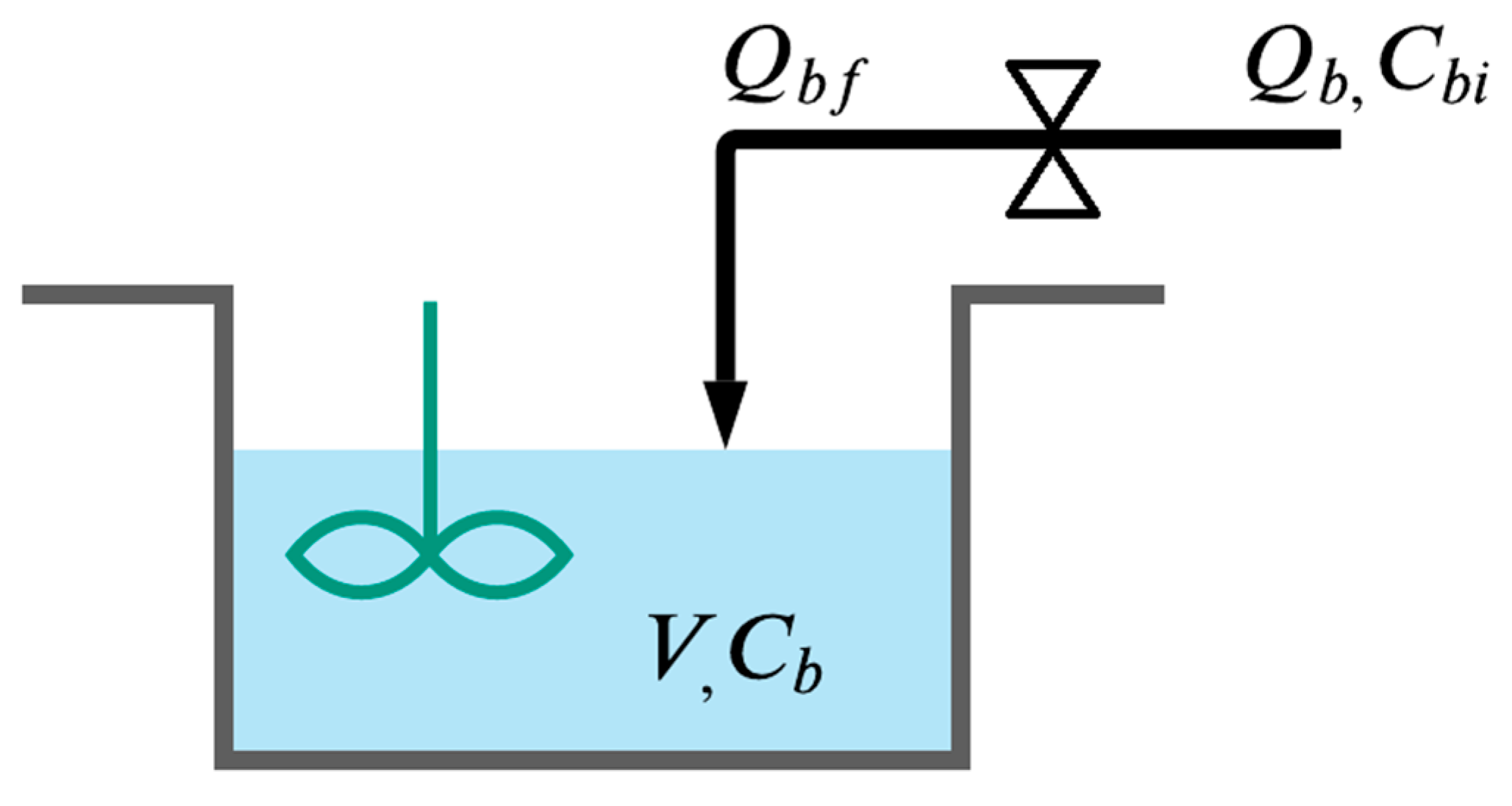
The effectiveness of the proposed observed-based controller is illustrated through simulation for control of base concentration in a batch reactor, with manipulation of the base flowrate. The batch reactor consists of a stirred tank of liquid volume (v) and base concentration, $C_b$, where a base flowrate ($Q_{bf}$) with concentration ($C_{bi}$) is added, but there are no other inflows or outflows, and the valve for base addition exhibits a linear input–output dynamics, with $Q_b$ being the base flowrate calculated by the controller and $Q_{bf}$ the actual value of the flowrate. The base concentration ($C_b$) is controlled by manipulation of the flowrate $Q_b$, with $Q_{bf}$ being unknown (see Figure 1).

The base concentration dynamics is based on mass balance on the tank (see Tan et al., 2005):

$$\frac{d{C}_b}{dt}=\frac{1}{v}\left(C_{bi}-C_b\right)Q_{bf}+{\delta }_{1a}$$

(98a)

$$\frac{dv}{dt}=Q_{bf}$$

(98b)

The valve dynamics describes the actual value of the flowrate ($Q_{bf}$) as function of the base flowrate calculated by the controller ($Q_b$) [51]:

$$\frac{d{Q}_{bf}}{dt}=-\frac{1}{{\tau }_v}{Q}_{bf}+\frac{1}{{\tau }_v}{Q}_b+{\delta }_{2b}$$

(98c)

where ${\tau }_v$ is the time constant of the valve dynamics. In addition, ${\delta }_{1a}$ and ${\delta }_{2b}$ are modeling errors, the volume is positive $(v>0)$, $C_{bi}$ is bounded and the ${\tau }_v$ is constant. This model corresponds to Model (1):

$$x_1=C_b, x_2=Q_{bf}, u=Q_b, b=\frac{1}{{\tau }_v}, f_{1ao}=-\frac{1}{v}\left(C_{bi}-C_b\right); f_{2o}=-\frac{1}{{\tau }_v}{x}_2; f_{1b}=0;f_{2c}=0$$

(99)

Moreover, the known value of b is $b_m=b$. From the valve dynamics (98c) and the bounded nature of flow $Q_b,$ it follows that $Q_{bf}$ is bounded, so that Assumption 1 is fulfilled. The uncertainty on the knowledge of $f_{1a0}$ is due to the uncertainty on the values of $C_{bi}$ and $v$:

$$f_{1a}=-\frac{1}{v_m}\left(C_{im}-x_1\right)$$

(100)

where $f_{1a}$ is the known value of $f_{1a0}$, $v_m$ is the known value of the volume $v$, and $C_{im}$ is the known value of $C_{bi}$. The values ($C_{im}$, $v_m$) satisfy: $v_m>0,$ $C_{im}\in L_{\infty }$. The uncertainty of $f_{1a}$ is as follows:

$${\delta }_{fa}={\delta }_{Iv}\left(C_{bi}-C_b\right)+\frac{1}{v}{\delta }_{cin}$$

(101a)

$${\delta }_{Iv}=\frac{1}{v}-\frac{1}{v_m}$$

(101b)

$${\delta }_{cin}=C_{bi}-C_{im}$$

(101c)

Recall that $v>0$, $v_m>0$, $C_{bi}$ and $C_{im}$ are bounded. Therefore, it follows from Equations (101b) and (101c) that ${\delta }_{Iv}$ and ${\delta }_{cin}$ are bounded, and consequently ${\delta }_{fa}$ (101a) is bounded:

$${\delta }_{fa}\le {\mu }_{fa}; {\mu }_{fa}=\max \left\{{\delta }_{Iv}\right\}\max \left\{C_{bi}\right\}+\frac{1}{\min \left\{v\right\}}\max \left\{{\delta }_{cin}\right\}$$

where ${\mu }_{fa}$ is constant, positive and unknown, so that the bounded nature of ${\delta }_{fa}$ considered in Assumption 3 is satisfied. From the valve dynamics (98c) and the bounded nature of Q, it follows that we achieve the following:

$$Q_{bf}\le u_{max} \mathrm{for} {Q_{bf}|}_{to}\le u_{max}$$

The equations of the formulated observer and controller are stated in Theorems 1 and 2, whereas the plant model terms are given by Equations (99) and (100). From Equation (98b), if follows that $v\approx {v|}_{to}$ if $Q_{bf}$ is small; thus, we consider this approximation. The values of the model parameters are ${\tau }_v=0.1 \min ,$ $u_{max}=0.2 \mathrm{L}/\min u_{min}=0 \mathrm{L}/\min \mathrm{and} {v|}_{to}=2 \mathrm{L}$:

$$C_{bi}={\overline{C}}_{bi}+A_{cbi}{\overline{C}}_{bi}sin\left(\frac{2\pi }{{\tau }_{cbi}}t\right), {\tau }_{cbi}=1\min , {\overline{C}}_{bi}=3 \mathrm{mol}/\mathrm{L}$$

$$c_{im}={\overline{C}}_{bi}; v_m=v$$

Two different simulation cases are considered:

-

In the first case, the command signal, $r$, is piecewise constant, the system is in open loop for $t\in \left[0 3\right]$min and we have the following:

$$A_{cbi}=0.05;{x_1|}_{to}=0.005; {u|}_{t\le 3 \min }=0.005 \left(open loop\right);$$

$$r=\{\begin{array}{c}0.01 for t\in \left(3 4.5\right) \min \\ 0.013 for t>4.5 \min \end{array}$$

-

In the second case, the command signal, $r$, is slowly time varying (its definition is discussed in Appendix A), the system is in open loop for $t\in \left[0 2\right]$min and we have the following:

$$A_{cbi}=0.08;{x_1|}_{to}=0; {u|}_{t\le 2 \min }=0.0 \left(open loop\right);$$

The chosen values for the observer and controller parameters are shown in

Table 1. Chosen parameter values for the observer and controller.

	Case 1	Case 2
Observer	$\epsilon =0.001; k_0=0.12;{\gamma }_a=1; {\gamma }_b=1.$	$\epsilon =0.003; k_0=0.2; {\gamma }_a=1; {\gamma }_b=1.$
Controller	$k_{c1}=0.0009; k_{c2}=1.0;$ ${\tau }_{T1}=0.001;k_f=0.001.$	$k_{c1}=0.00005; k_{c2}=0.4;$ ${\tau }_{T1}=0.001;k_f=0.0031.$

. The main differences between the first and second simulation cases are as follows: (i) in the first case, the command signal, $r$, is piecewise constant, whereas, in the second case, it is slowly time varying; (ii) in the first case, the width of the uncertainty on the influent base concentration $A_{cbi}$ is 0.05, whereas, in the second case, it is 0.08, what implies a higher uncertainty on $C_{bi}$ in the second case; and (iii) the values of the observer parameter, $k_0$, and the controller parameter, $k_f,$are higher in the second case, whereas the controller parameters $k_{c1} \mathrm{and} k_{c2}$ are higher in the first case, allowing us to illustrate that the used parameter values are proper for obtaining convergence of the tracking error.

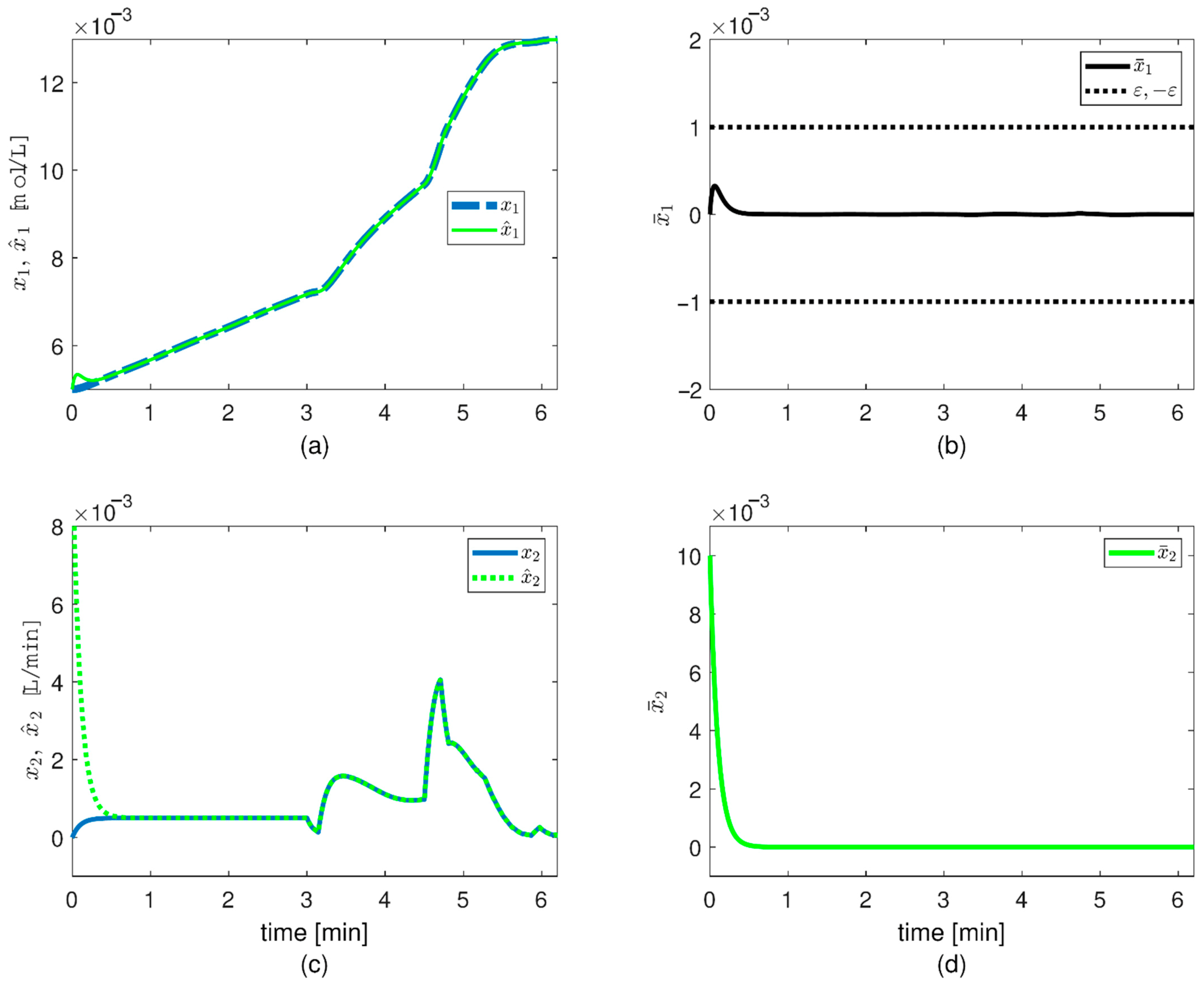
The first case observer simulation case shows that (Figure 2) (i) the estimate ${\widehat{x}}_1$ tracks $x_1$ (Figure 2a), (ii) the observer error ${\overline{x}}_1={\widehat{x}}_1-x_1$ remains in the compact set ${\Omega }_{\overline{x1}}=\left\{{\overline{x}}_1:\left|{\overline{x}}_1\right|\le \epsilon \right\}$ (Figure 2b) and (iii) the estimate ${\widehat{x}}_2$ tracks $x_2$ (Figure 2c). In addition, the estimated parameter, $\widehat{\theta }$, remains bounded with no excessive increase (data not shown).

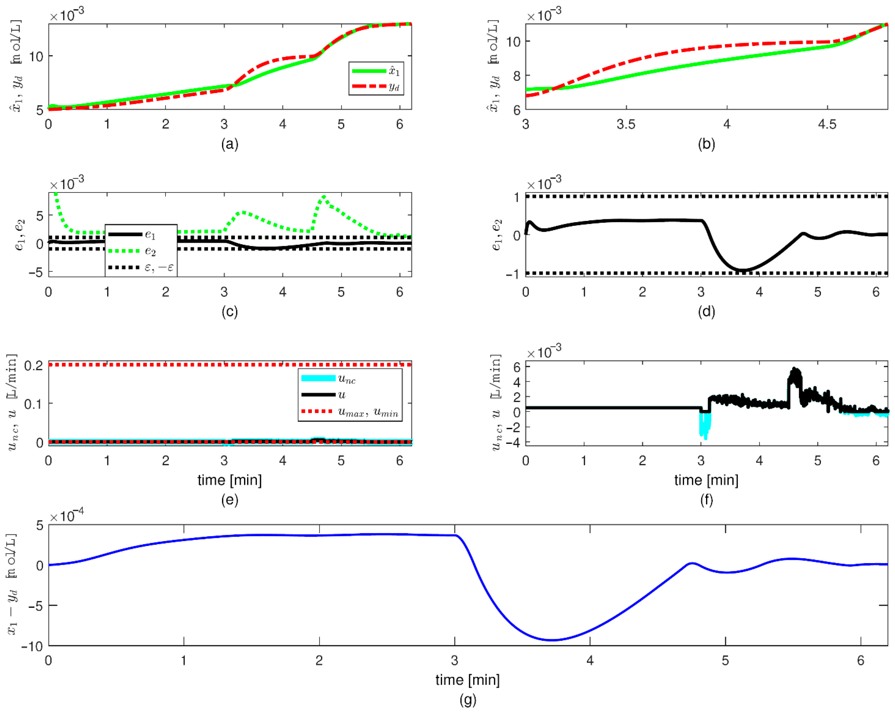
The first case simulations of the controller show that (Figure 3) (i) ${\widehat{x}}_1$effectively tracks y_d (Figure 3a,b), (ii) the tracking error $e_1={\widehat{x}}_1-y_d$ remains in the compact set ${\Omega }_{e1}=\left\{e_1:\left|e_1\right|\le \epsilon \right\}$ (Figure 3c,d) and (iii) there is a fast response of the control input to changes in the error $e_1$ (Figure 3e,f).

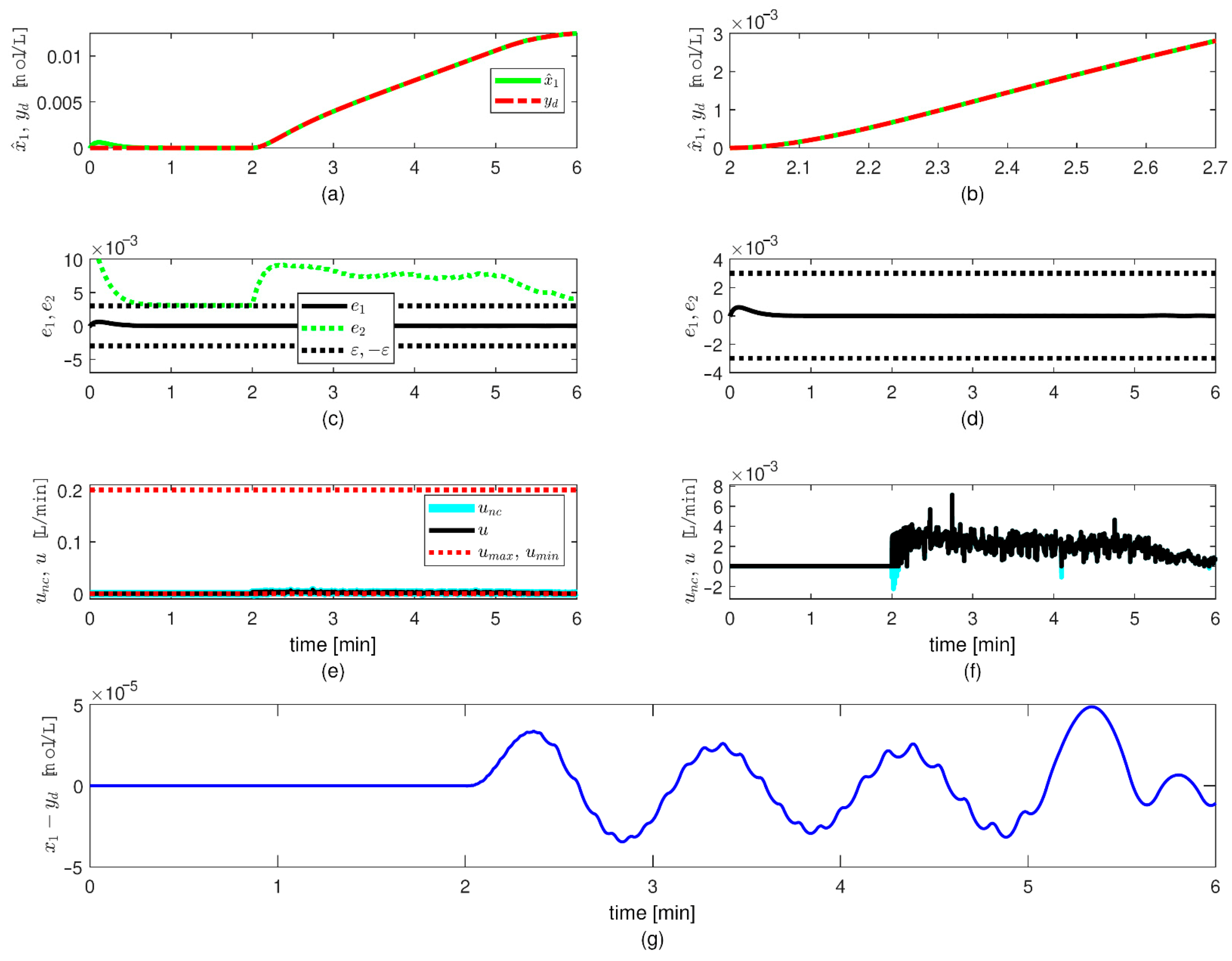
The second case simulations of the controller show that (Figure 4) (i) ${\widehat{x}}_1$effectively tracks y_d (Figure 4a,b), (ii) the tracking error $e_1={\widehat{x}}_1-y_d$ remains in the compact set ${\Omega }_{e1}=\left\{e_1:\left|e_1\right|\le \epsilon \right\}$ (Figure 4c,d) and (iii) there is a fast response of the control input to changes in the error $e_1$ (Figure 4e,f).

The observer error ${\overline{x}}_1={\widehat{x}}_1-x_1$ remains inside ${\Omega }_{\overline{x1}}$, so that $f_{v1}$ remains equal to zero, for both the first and second cases (Figure 2b). Due to this fact and the dependence of the update law (55) on $f_{v1}$, the updated parameter vector $\widehat{\theta }$ remains constant and equal to its initial value (data not shown). The main features of the tracking error $e_1={\widehat{x}}_1-y_d$ are as follows: (i) it remains inside ${\Omega }_{e1}$ for both the first and second cases (Figure 3c,d and Figure 4c,d), so that undesired large transient values are avoided; (ii) it is lower in the second case, which indicates that the controller parameter, $k_f$, has a significant effect on the value of the control input signal, and consequently on the tracking performance. Since the observer error, ${\overline{x}}_1$, and the tracking error, $e_1$, remain each inside a compact set whose width is $\epsilon$, the error $x_1-y_d$ (Figure 3g and Figure 4g) remains inside a compact set of small size.

The control effort remains relatively low, with only a few moments of input saturation (Figure 3e,f and Figure 4e,f). This is achieved by using no overly large controller parameters,$k_{c1}, k_{c2} \mathrm{and} k_f$. The control input achieves noticeable changes of the system output in 0.3 min (Figure 2a,c), but this depends on the input–output dynamics of the system and the control law.

6. Conclusions

In this paper, we proposed a robust observer-based adaptive controller for systems described by second-order input–output dynamics with unknown second state, and it was applied to concentration tracking in a chemical reactor. The controller design was improved so as to achieve faster response of the control input to the output tracking error, while providing robustness against disturbance terms or modeling errors, avoiding input chattering. The improved sensitivity of the control input is provided through a new saturation function of the output tracking error. To this end, several modifications were incorporated in the backstepping method, including a different definition of the second backstepping state. The advantages over current observer based controllers for second-order models are (i) discontinuous signals are avoided in the control law, the update law and the observer equations; (ii) the width of the convergence region of the tracking error does not depend on upper bounds of either model terms, state variables or disturbances; and (iii) the control law exhibits an enhanced speed of response to changes in the tracking error, whereas the control effort can be reduced through the controller parameters. The simulations show the aforementioned advantages of the formulated controller, including (i) fast convergence of the output to the desired value; (ii) fast response of the input signal to changes in the output error; (iii) continuous behavior of the input signal, with no chattering; and (iv) no excessive control effort.