
Response of Viscoelastic Turbulent Pipeflow Past Square Bar Roughness: The Effect on Mean Flow


Department of Mechanical Engineering, University of Alberta, Edmonton, AB T6G 2R3, Canada
*
Author to whom correspondence should be addressed.
†
These authors contributed equally to this work.
Computation 2021, 9(8), 85; https://0-doi-org.brum.beds.ac.uk/10.3390/computation9080085
Submission received: 21 May 2021
/
Revised: 26 July 2021
/
Accepted: 28 July 2021
/
Published: 30 July 2021
(This article belongs to the Section Computational Engineering)
Abstract
:The influence of viscoelastic polymer additives on response and recovery of turbulent pipeflow over square bar roughness elements was examined using Direct Numerical Simulations at a Reynolds number of . Two different bar heights for the square bar roughness elements were examined, and . A Finitely Extensible Non-linear Elastic-Peterlin (FENE-P) rheological model was employed for modeling viscoelastic fluid features. The rheological parameters for the simulation corresponded to a high concentration polymer of 160 ppm. Recirculation regions formed behind the bar elements by the viscoelastic fluid were shorter than those associated with Newtonian fluid, which was attributed to mixed effects of viscous and elastic forces due to the added polymers. The recovery of the mean viscoelastic flow was faster. The pressure losses on the surface of the roughness were larger compared to the Newtonian fluid, and the overall contribution to local drag was reduced due to viscoelastic effects.
1. Introduction
Response and recovery of turbulent pipeflow to abrupt surface variations, i.e., roughness elements, is a fundamental study of non-equilibrium flow behaviour with various industrial and engineering applications. For example, extraction and transport of various heavy crude and petroleum products are routinely carried out using pipelines [1]. The flow in most crude transport pipelines experiences small eddies and near-wall turbulence, which increases frictional drag. This incurs heavy energy losses in the transport of highly viscous fluids like crude or heavy-oil bitumen [2]. Thus, techniques for frictional drag reduction are of significant practical interest. It has been established that the addition of high molecular-weight non-Newtonian polymers in turbulent pipeflow produced upward of drag reduction, and it significantly reduced turbulent frictional drag on the pipe walls [3,4]. This phenomenon was first reported by Toms (1948) [5], and such polymer additives were named Drag-Reducing Agents (DRAs). The addition of such polymers led to the fluid experiencing elastic viscosity as well as Newtonian viscosity; hence, they are referred to as viscoelastic fluids [6]. Polymer additives for purposes of drag reduction have been used successfully in many applications including the transport of crude in pipelines [7], energy saving transport medium in residential heating devices [8], as well as sewer [9], firefighting systems [10], and hydrodynamic systems [11].
Transport of energy-related fluids through pipes and channels involves a high Reynolds number, and in most practical cases, includes turbulent flows over rough surfaces. Abrupt surface variations at high Reynolds numbers constitute a class of non-equilibrium or perturbed flows, which have been the focus of extensive research using Newtonian fluids. The behaviour of such flows is typically complex because the perturbations or step changes cause contraction in the flow, particularly at a high Reynolds number. There are several studies that investigate different aspects of Newtonian fluid flow past wall-mounted obstacles or perturbations, and non-equilibrium flow conditions. Smits et al. (1979) [12] studied the effects of abrupt surface variations on flow recovery and observed a second-order response, which led to long-lasting changes in the turbulent structures in the flow. This was followed by the study of Durst and Wang (1989) [13], who investigated, experimentally and numerically, the flow response to an axisymmetric perturbation. They found an overshoot of flow response in the vicinity of the perturbation due to the mixed effects of sudden contraction and expansion, as opposed to sudden expansion in the flow over a backward facing step. Dimaczek et al. (1989) [14] observed similar effects for wall-mounted axisymmetric perturbations over a wide range of Reynolds numbers. Studies of Jiménez (2004) [15] and Smits et al. (2019) [16] focused on turbulent flow over small step conditions or roughness elements, defined by the ratio of the lateral width of the object (h) with respect to the boundary layer width (), given as . These small step conditions were unique in terms of their effects on the overall flow response and downstream recovery. Smits et al. (2019) [16] studied the flow response and recovery over two roughness heights of and at Reynolds number of using Particle Image Velocotimetry (PIV). This study identified that the sudden contraction and expansion of the incoming flow resulted in longer reattachment lengths and amplification of the Reynolds stresses near the vicinity of the roughness element. For larger roughness elements, the downstream collapse of Reynolds stresses was sudden, whereas it extended far downstream for smaller roughness elements.
Extensive studies have looked at the effects of multiple, tandem wall-mounted structures on flow response and overall flow dynamics. Leonardi et al. (2003) [17] studied the flow response over tandem wall-mounted square bars, over a range of periodic separation ratios. It was determined that for large separation between two obstacles, the recirculation length was altered by the adverse pressure gradient imposed by the upstream wall of the subsequent object. Such flow behaviour was analogous to the study of wake characteristics behind flat plates by Hemmati et al. (2019) [18]. This was followed by the study of Goswami and Hemmati (2020) [19], who investigated the effects of turbulent flow over multiple roughness elements and different separation patters on the flow response and recovery. They considered two roughness element heights of and , as well as two separation patterns: periodic and staggered. It was determined that the flow recovery was prolonged by the use of smaller roughness elements, while the separation patterns had negligible effects on the overall response and recovery as long as the elements are positioned outside the impinging zone of the upstream element. Further, Goswami and Hemmati (2021) [20] investigated the Reynolds number effects and scaling on the response and recovery of the flow over the roughness elements. They considered a square bar roughness element of and Reynolds numbers between and . They observed an asymptotic trend in the reattachment lengths with increasing the Reynolds numbers, while the recovery trends followed a power-law behaviour of diffusion towards the centerline. Furthermore, the collapse of stresses towards the wall appeared earlier at low Reynolds numbers. While the studies on Newtonian flow past wall-mounted obstacles are abundant, viscoelastic fluid flow over such conditions has received limited attention despite its extensive industrial applications.
The numerical studies on viscoelastic flows mainly used Direct Numerical Simulations (DNS) [21,22,23,24,25] and Reynolds-Averaged-Navier–Stokes (RANS) turbulence models [26,27]. Experimentally, Particle Image Velocimetry (PIV) [28,29] and Laser-Doppler-Velocimetry (LDV) [30,31] were used to characterize the flow. Experimental studies mainly focused on investigating turbulence statistics, structure of polymeric flow, and the study of elastic instabilities over a wide range of sub-critical Reynolds numbers. Numerical studies used DNS with one or more non-linear differential models such as Oldroyd-B model [32], Giesekus model [33], Phan-Thein-Tanner (PTT) model [34], and Finitely Extensible Non-linear Elastic-Peterlin (FENE-P) model [35]. These studies were limited to lower Reynolds numbers because of the complexities in terms of modeling various rheological behaviour of the fluid and resolving various non-linear viscous and elastic effects [36]. Earlier numerical studies using DNS and several viscoelastic models were limited to smooth pipes, plane channel, and boundary layers. Azziez et al. (1996) [24] studied Giesekus, PTT and FENE-P models in simulating flow through 4:1 planar contraction. By comparing the performance of different rheological models with the experimental results, it was determined that the FENE-P model performed the best overall in terms of predicting the pressure drop, shear and normal stresses and drag reduction. This was followed by the work of Sureshkumar et al. (1997) [37], who demonstrated the first DNS channel flow using a viscoelastic fluid and FENE-P constitutive model. This study was performed at lower Reynolds numbers and a range of Weissenberg numbers (, a dimensionless number characterizing the flow elasticity) to benchmark a set of criteria for onset of drag reduction in plane channel flows. The Finitely Extensible Non-linear Elastic (FENE) model was first proposed by Warner and Harold (1972) [38], as a solution to the gaps in the linear spring model that had no restriction on the deformation of the polymer chain. This was further extended by Bird et al. (1987) [35], who proposed the FENE-P model with Peterlin closure approximation. Here, the finite extension of the polymer chains was restricted by the parameter , which is the dimensionless extensibility of the polymer chain. Since many such studies have complimented its accuracy and compatibility with numerical simulations, the FENE-P constitutive model is currently the most appropriate model for complex flow simulations.
Rothstein and McKinley (2001) [39] investigated the flow of polystyrene-added fluid through contraction–expansion geometry of varying expansion ratios using LDA. They studied the effects of contraction-expansion geometries on the pressure drop due to flow contraction and wake characteristics. They determined that while the addition of polymer-additive in the fluid does reduce the overall pressure and skin-friction drag, the intensity of such reduction vastly depends on the concentration of the added polymer. This was followed by Poole and Escudier (2003) [40], who investigated the influence of different polymer concentrations on the turbulent flow through sudden planar expansion using transverse LDA with a linear expansion ratio of . They observed that the reattachment lengths by low polymer-concentration fluids increased, while for higher concentrations, it decreased significantly. The lower reattachment length was accompanied by a large reduction in turbulent intensity occurring at the point of flow separation for higher concentration solutions. Oliveira (2003) [41] further numerically investigated the effects of axisymmetric abrupt expansion geometries using FENE rheological models for low Reynolds numbers and a range of , polymer extensibility and concentrations. The results showed similarities with the findings of Poole and Escudier (2003) [40], combined with a reduced pressure and skin-friction distribution along the walls. Further, Poole et al. (2007) [42] performed experiments on viscoelastic flow over a backward-facing step with varying polyacrylamide-concentration solutions at Reynolds numbers of 10–100. It was determined that as the polymer concentration increases, the combined effects of shear-thinning and viscoelasticity lead to reduced reattachment lengths behind the step, while an overshoot of velocity was observed compared to Newtonian fluid.
In recent years, there have been several studies that investigate the effects of viscoelastic polymer additives on flow past bluff bodies and wall-mounted obstacles, as well as on the implications of viscoelasticity on large-scale and very-large scale motions. Xiong et al. (2013) [43] carried out numerical simulations of two-dimensional flow past a circular cylinder using multiple rheological models and varying Reynolds number, Weissenberg number and polymer concentrations. An overshoot of velocity gradients and stresses were observed in the vicinity of the cylinder at high polymer conversations, while the intensities of the overshoot were very low compared to Newtonian fluid. Further, as the Reynolds number increased, vortex shedding was observed for the Newtonian fluid, which reduced gradually with increasing polymer concentrations and numbers. Tsukahara et al. (2014) [44] performed DNS simulations of turbulent viscoelastic flows in a channel with wall-mounted plates and studied the influence of viscoelasticity on turbulent structures and large-scale motions behind the wall-mounted plates. They observed that for the Newtonian fluid, three pairs of large-scale vortices occur behind the plates, which was significantly weakened in the viscoelastic fluid. This suppression of vortices was influenced by the elastic and viscous forces, which resulted in a significant reduction of drag behind the plate and a decreased skin-friction on the surface of the plate. They also observed a slight increase in reattachment lengths behind the plate with lower polymer concentrations and a reduction at higher concentrations. These findings were in agreement with those of Tsukahara et al. (2013) [45] and Poole and Escudier (2003) [40], who provided evidence of the mixed effects of elastic and viscous forces.
While investigations such as those of Dubief et al. (2013) [25] and Shaban et al. (2018) [29] extensively study the mechanisms of turbulent viscoelastic plane channel flows and smooth pipes, limited studies exist that investigate these effects with abrupt surface variations at high Reynolds numbers. Furthermore, viscoelastic flows past roughness elements and small-step () conditions have not gained sufficient attention. Here, we examine the effects of viscoelastic fluid on flow over square bar roughness elements using a DNS and FENE-P rheological constitutive model at Reynolds number of . Particularly, we investigate the influence of higher-polymer concentration viscoelastic fluid on the flow response and recovery over perturbed flow conditions. For clarity, the results are compared with Newtonian flow over roughness element at the same Reynolds number. This paper is prepared in such a way that the problem description in Section 2 is followed by a discussion of results in Section 3 and conclusions in Section 4.
2. Problem Description
We examined the response and recovery of Newtonian and non-Newtonian turbulent fluid flow over square bar roughness elements of two different heights using DNS at Reynolds number of . First, the simulations were carried out using water, a Newtonian fluid, as a benchmark simulation. This was followed by examining the effects of viscoelastic polymer additives using a FENE-P rheological model incorporated into DNS. Finally, the results of viscoelastic simulations were compared with those of Newtonian DNS simulations to study the implications of viscoelastic fluid on the overall flow dynamics, response and recovery.
The governing equations for incompressible fluids are the continuity equation and the momentum equation, given by
where u is the velocity vector, is the fluid density, p is the isotropic pressure and is the stress tensor. For Newtonian DNS simulations, the continuity (Equation (1)) and momentum (Equation (2)) equations were solved directly. For viscoelastic simulations, however, the stress tensor was split into a solvent or Newtonian stress component () and a non-Newtonian or polymeric stress component (), such that
The Newtonian stress component is defined as , where is the solvent viscosity and is the rate-of-strain tensor given by
Substituting this into Equation (2) gives a modified momentum equation:
where is defined in the multimode from () as a symmetric tensor () obtained by the sum of the contributions of individual relaxation modes. The majority of viscoelastic materials are composed of molecular structures of different sizes, and therefore they have different relaxation times. The multimode formulation enables the inclusion of a vast spectrum of relaxation times to obtain more realistic results. The expression of depends on the viscoelastic constitutive equations employed. For viscoelastic simulations here, the polymeric stress tensor was computed using the FENE-P model constitutive equation [35] as follows,
where is the polymer relaxation time, is the extensibility of the polymer molecule, tr() is the trace of the polymer stress tensor, and is the upper convected derivative given as
and is the total derivative of the polymer-stress tensor, defined as
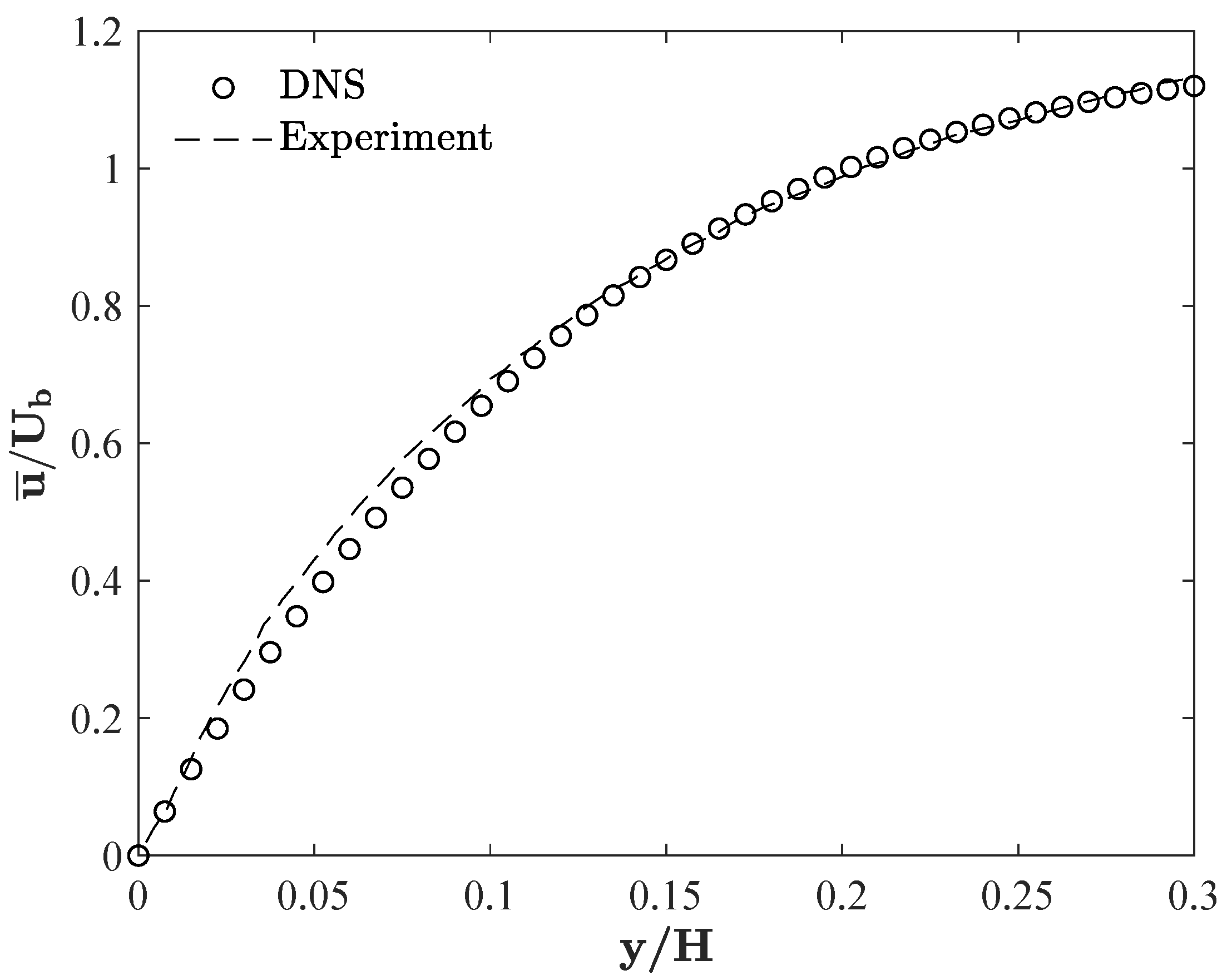
The simulation setup in the current study mimicked those of Favero et al. (2010) [21] and Holmes et al. (2012) [23], both of which incorporated the FENE-P rheological model in DNS using OpenFOAM. They then proceeded with verifying and validating the accuracy of this model. The FENE-P model was further validated by Dubief et al. (2013) [25] in studying elasto-inertial turbulence. To this effect, we simulated the experimental channel flow of Shaban et al. (2018) [29] by incorporating the FENE-P model into DNS in OpenFOAM, which showed a good agreement in Figure 1. Hereon forward, the overbar symbol (, where is any flow parameter) identifies time-averaged results. The grid spacing for the simulation was , the Weissenberg number () was , the polymer extensibility () was 200 and the viscosity ratio, , was , consistent with the experiments.
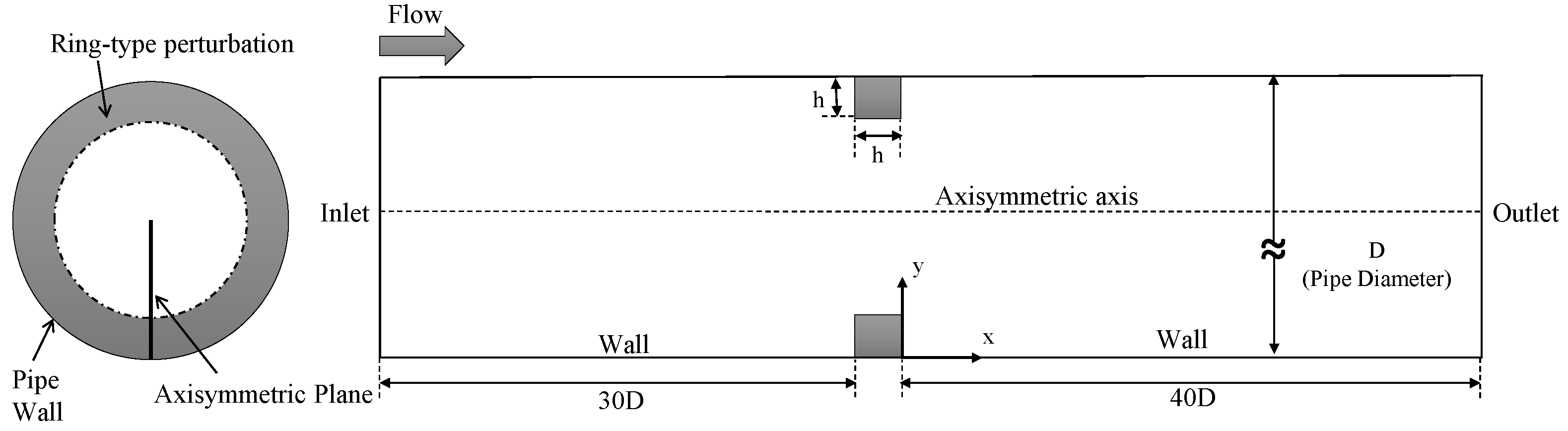
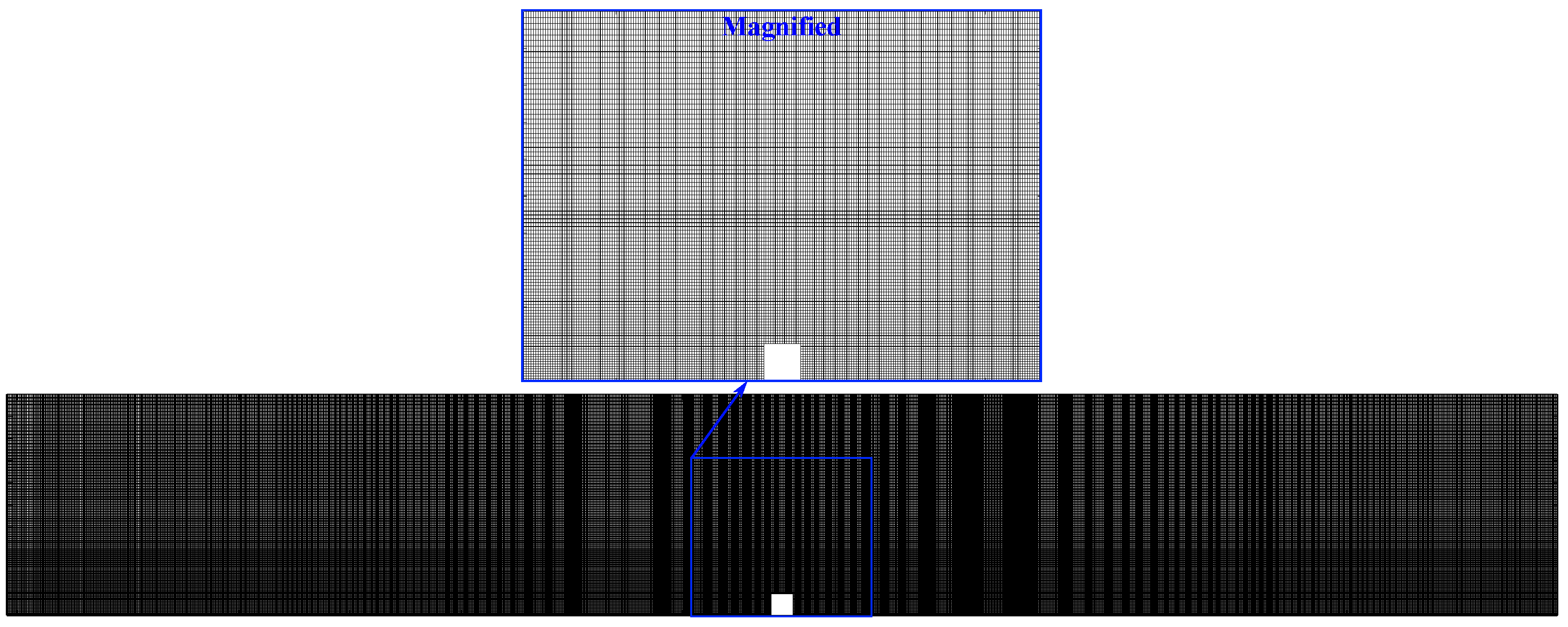
The schematics of the axisymmetric computational domain, as shown in Figure 2, was designed following the setup of Smits et al. (2019) [16] and Yamagata et al. (2014) [46], which was verified by Goswami and Hemmati (2020, 2021) [19,20] to properly capture the main features of the geometrically-symmetric pipe flow. The axisymmetric perturbation was introduced by placing a square cross section ring with heights of and in the pipe. Here, the square bar roughness element has a height of h, and the inner diameter of the pipe is D. All simulations were performed based on an axisymmetric assumption. The domain extended from to in the direction, and in the direction. A non-homogeneous spatial grid with a total of hexahedral elements was used to discretize the domain. The grid distribution was such that the fine mesh was placed close to the wall boundaries, as shown in Figure 3. The minimum spatial grid requirement for a DNS simulation was satisfied by coinciding with the order of magnitude of element size, , with the order of magnitude of the Kolmogorov length scales, , at the pipe walls and in the vicinity of the roughness element. The Kolmogorov length scales are calculated using , based on Newtonian fluid viscosity, where is the mean dissipation rate calculated using the approximation of . Table 1 shows the grid resolution of the current grid as a variation of in the axial direction up to . The was less than 4 at least up to , while near the vicinity of the roughness element, they were below ∼2. These ratios were comparable to other DNS studies on wakes [47] and viscoelastic pipeflows [25,48].
The parameters used in the simulations are given in Table 2. For all viscoelastic simulations, the non-dimensional extensibility () and parameter were fixed at 200 and 0.22, where is defined as the ratio of solvent viscosity to the zero-shear viscosity of the polymer solution, given by . The parameter was selected such that we obtain a shear-thinning solution behaviour. Further, the corresponding polymer concentration of 160 ppm availed lowering of the solution viscosity, which enables the shear-thinning fluid behaviour analyzed in this study, as well as allowing for a higher drag reduction [29]. is the polymer relaxation time, which was obtained experimentally by Shaban et al. (2018) [29] for a solution of polyacrylamide polymer at 160 ppm. The simulations were performed at , defined by pipe diameter (D) and bulk velocity () across the pipe. Using the friction factor correlation given by Mckeon et al. (2004) [49], the upstream friction velocity corresponded to the friction Reynolds number of . The Reynolds number based on the square bar height and solvent viscosity was 250 and 500, and the linear expansion ratios were for and for .
Identical boundary conditions were used for all the simulations. The inlet boundary condition was a constant uniform velocity, . The separation distance between the inlet and the roughness element was kept sufficiently long to satisfy the hydrodynamic entrance length condition at this Reynolds number. A Neumann-type outflow condition based on , where is any flow variable, was imposed at the outlet, and a no-slip type boundary condition was imposed at the walls and the roughness element. The timestep, , for all simulations was set so that the maximum Courant–Friedrichs–Lewy (CFL) number remained below 0.8 for Newtonian simulations and 0.2 for viscoelastic simulations. The smaller timestep requirement for viscoelastic simulations guarantees the boundedness of [25]. All simulations were performed using OpenFOAM, an open-source finite-volume-method platform. All discretized equations were solved using PimpleFoam, a transient solver for incompressible, turbulent flow. PimpleFoam solver incorporates the PIMPLE algorithm [50], which is the combination of PISO (Pressure Implicit with Splitting of Operator) and SIMPLE (Semi-Implicit Method for Pressure-Linked Equations) algorithms. The second-order accurate and bounded numerical discretization schemes for spatial discretization and the backward Euler scheme for temporal discretization were employed for the simulations. The convergence criterion of was set for the root-mean-square of momentum residuals, for each timestep. The convergence was guaranteed by running all simulations for ten through-times, where a through-time is defined as the time fluid takes to travel from inlet to outlet without any disturbance. All simulations were completed using 48 Intel Platinum 8160 F Skylake 2.1 GHz cores and 192 GB of memory, using core hours on Compute Canada clusters.
3. Results and Discussion
We begin by looking at the viscoelastic fluid flow response over the square bar roughness element. The Newtonian fluid flow simulation is our base flow to establish the differences due to non-Newtonian fluid effects. This is followed by the investigation of flow recovery and the distributions of pressure and wall shear stresses by the viscoelastic fluid.
3.1. Flow Response
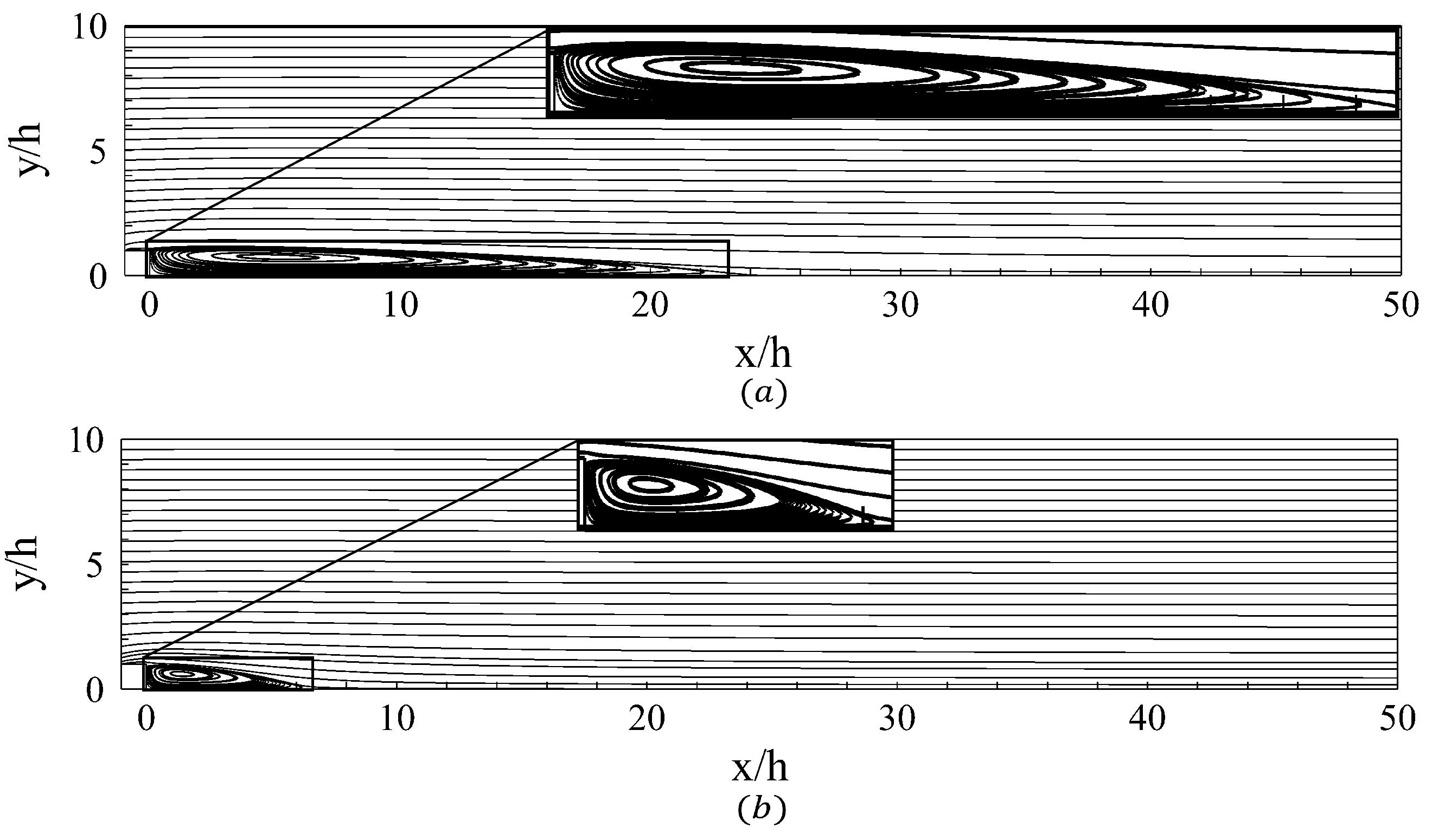
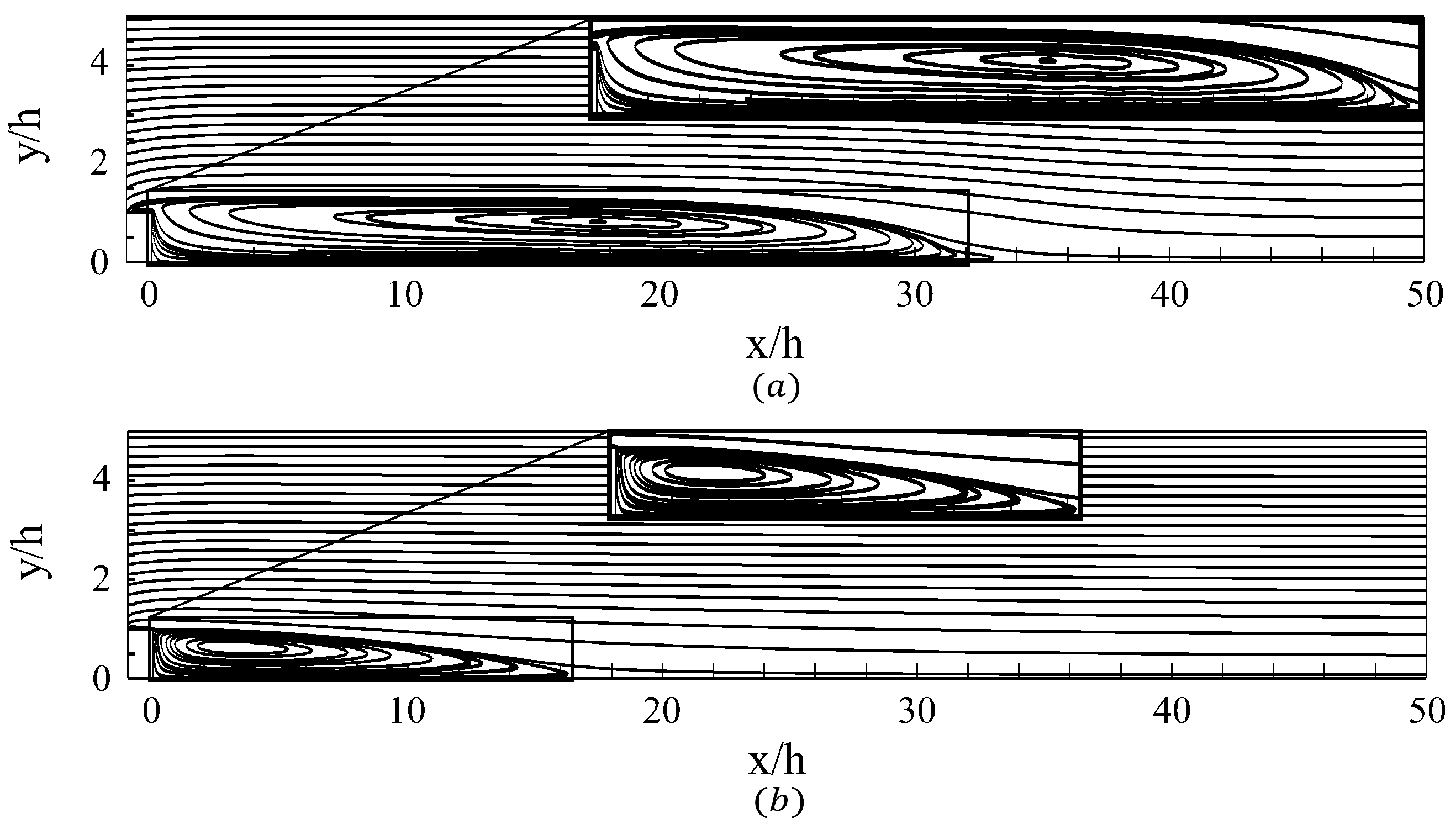
The flow response was evaluated by analyzing the nature of mean wake features behind the roughness element. Figure 4 and Figure 5 show the mean streamline plots for Newtonian and viscoelastic fluid for two roughness heights. For all cases, the flow separation occurred at the upstream edge of the roughness element, followed by the formation of a recirculation bubble before the flow reattaching to the bulk flow in the downstream region of the roughness element. From the first glance, it was evident that the longitudinal width (length) of the separation bubble for viscoelastic fluid in Figure 4b and Figure 5b was significantly smaller than that of the Newtonian fluid in Figure 4a and Figure 5a, respectively. Furthermore, the lateral width (height) of the recirculation bubble exceeded that of the roughness element by ∼5% for and ∼15% for in the case of the Newtonian fluid. For viscoelastic fluid, however, the lateral width of the recirculation bubble did not exceed the height of the roughness element for both bar heights.
A quantitative comparison of the recirculation lengths obtained from Newtonian and viscoelastic flow past a roughness element is shown in Table 3. For the smaller roughness height, the mean recirculation length formed by the viscoelastic fluid exhibited a difference of ∼73% from that of the Newtonian fluid. For the larger roughness height, the observed difference was ∼50%. For Newtonian fluid, the reattachment length differed between the two bar heights by ∼32%. Since the larger bar element () created a larger contraction in the flow, it led to a larger pressure gradient compared to that of the smaller square element. Thus, both the recirculation bubble and the reattachment length were larger for Newtonian flow over roughness element of height compared to the smaller element. Viscoelastic fluid, on the contrary, suppressed the velocity gradients in the vicinity of the roughness element, due to which the effects of large pressure gradients were diminished. This led to a shorter recirculation length compared to that of the Newtonian fluid.
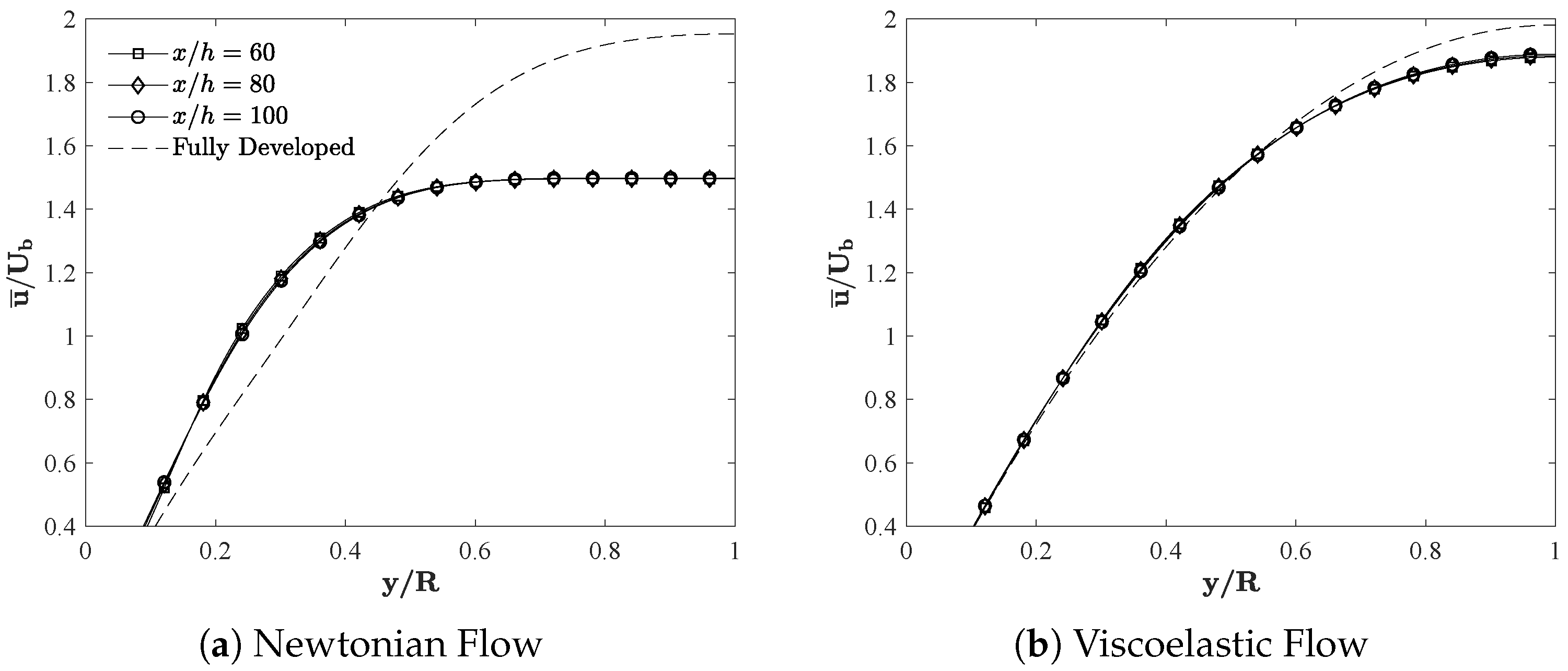
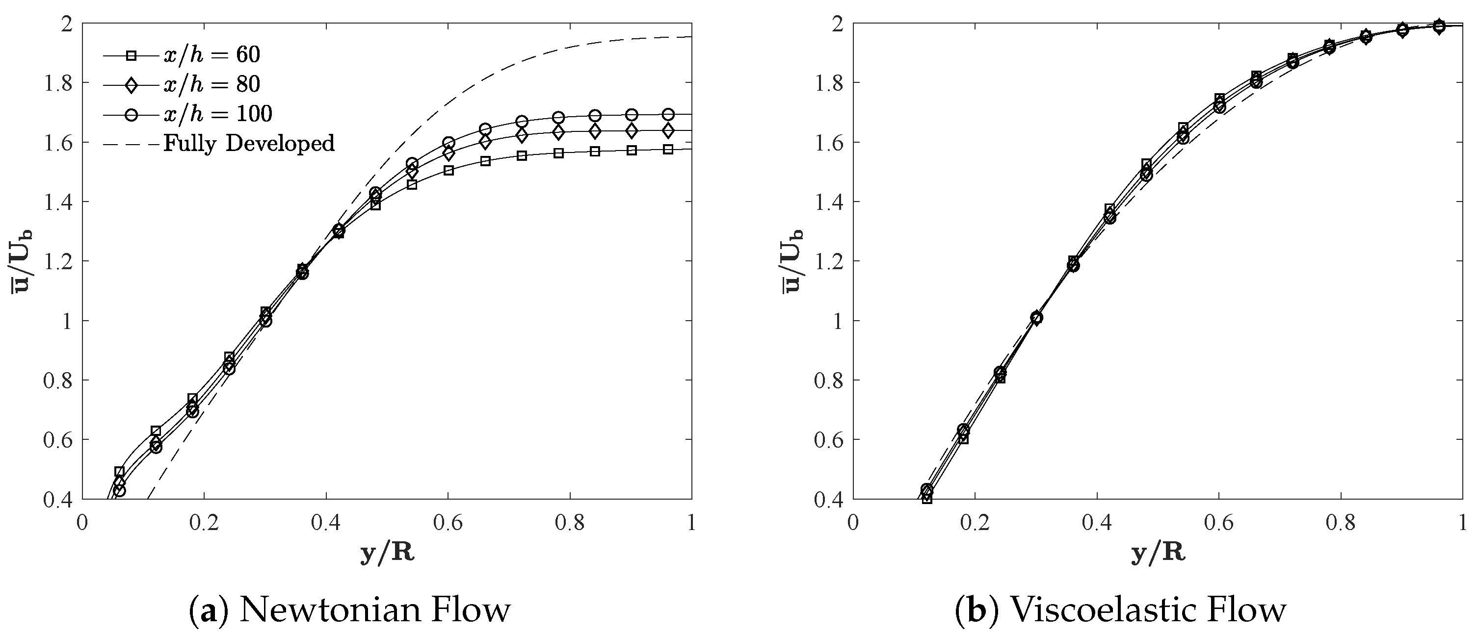
The profiles of mean axial velocity obtained from Newtonian and viscoelastic fluids are shown in Figure 6 and Figure 7 for and , respectively. Profiles are plotted at three different axial locations downstream of the roughness elements: and 100. For Newtonian fluid (Figure 6a and Figure 7a), the profiles for different bar height cases were quite distinct. In the case of , the velocity near the centre at was ∼30% below the fully developed profile. As the flow progressed, the variations at became negligible near the centre, while slight variations (∼0.2%) were observed closer to the wall. In contrast, velocity profiles for showed faster progression towards the fully developed profiles with ∼5% difference at the centre between and 100. Smits et al. (2019) [16] stated that the velocity for a smaller roughness element exceeded the fully developed profile, while that of a larger roughness element was over-flattened by Reynolds shear stresses. The trends of velocity profiles observed here contrasted the trends observed by Smits et al. (2019) [16] at , which hinted at the effects of the Reynolds number on the flow dynamics and scaling. This finding agreed with experiments of Hultmark et al. (2012) [51], who recorded similar effects in pipeflow with velocity in the centre of the pipe scaling with increasing Reynolds number. The study of Goswami and Hemmati (2021) [20] showed that the flow response and recovery scaled with changing Reynolds number and observed a reduced mean centerline velocity with increasing the Reynolds number, which was consistent with the observation of the current study.
In the case of viscoelastic fluids (Figure 6b and Figure 7b), velocity profiles vastly differed from the trends observed for Newtonian cases. For both bar heights, velocities appeared to have recovered close to fully developed profiles as early as . For , the velocity at was slightly (∼2.5%) below that of the fully developed profile. As the flow progressed between and 100, the variation in velocity was negligible, showing a trend similar to that of Newtonian flow over the smaller roughness element (). In the case of a larger square bar, velocity close to the center of the pipe () appeared to recover to a fully developed profile, while slight variations were observed in . The lower free-shear Reynolds number for the viscoelastic flow hinted at laminarization effects as a result of significantly reduced solution viscosity to favour shear-thinning effects. Thus, the profiles of velocity appeared to be laminar, while the peak velocities remained high.
3.2. Flow Recovery
The mean flow recovery was compared between the Newtonian and viscoelastic flows by locating the axial position where the profiles appear to approach an equilibrium state or the fully-developed state. The recovery location, , was assumed if the consecutive variations in the flow gradients in the axial (streamwise) direction were less than . The results in Table 4 show the recovery locations, , for both Newtonian and viscoelastic flow and both roughness heights. The mean Newtonian flow recovered within for and for . The mean flow recovery of the smaller roughness element was prolonged, while that of the larger element was accelerated. These observations are consistent with the study of Goswami and Hemmati (2020) [19]. Similarly, mean viscoelastic flow recovered within for and for . Comparable to the Newtonian flow counterpart, the mean viscoelastic flow showed faster recovery with , while a prolonged recovery by .
For , the mean axial flow showed an accelerated recovery, ∼71% faster for the viscoelastic flow compared to the Newtonian flow. Similarly to , the viscoelastic flow recovered ∼70% faster compared to the Newtonian flow. This hinted at an accelerated recovery for viscoelastic flows compared to Newtonian flow, which may be attributed to the effect of reduced fluid viscosity due to the addition of the polymeric additive, resulting in the shear-thinning effects and faster mean flow recovery.
3.3. Distribution of Pressure and Wall Shear Stresses
Effects of viscoelasticity on the flow characteristics and the roughness element were more clearly illustrated in the distributions of pressure and skin friction. First, the contribution of skin friction and pressure drag were examined on the overall local drag acting on the perturbation surfaces. The distribution of pressure and wall shear stresses were defined by pressure coefficient () and skin friction coefficients (), respectively. The coefficient of pressure is given as
where is the static pressure of the incoming flow. Similarly, the skin friction coefficient is given as
where is the wall shear stress.
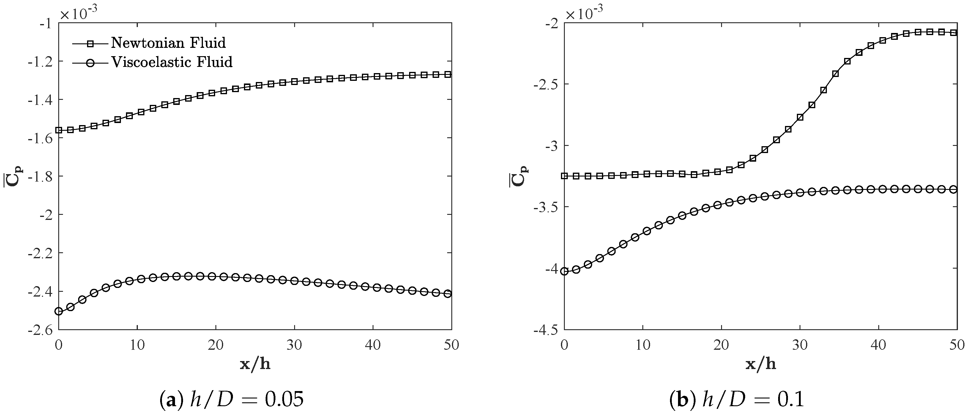
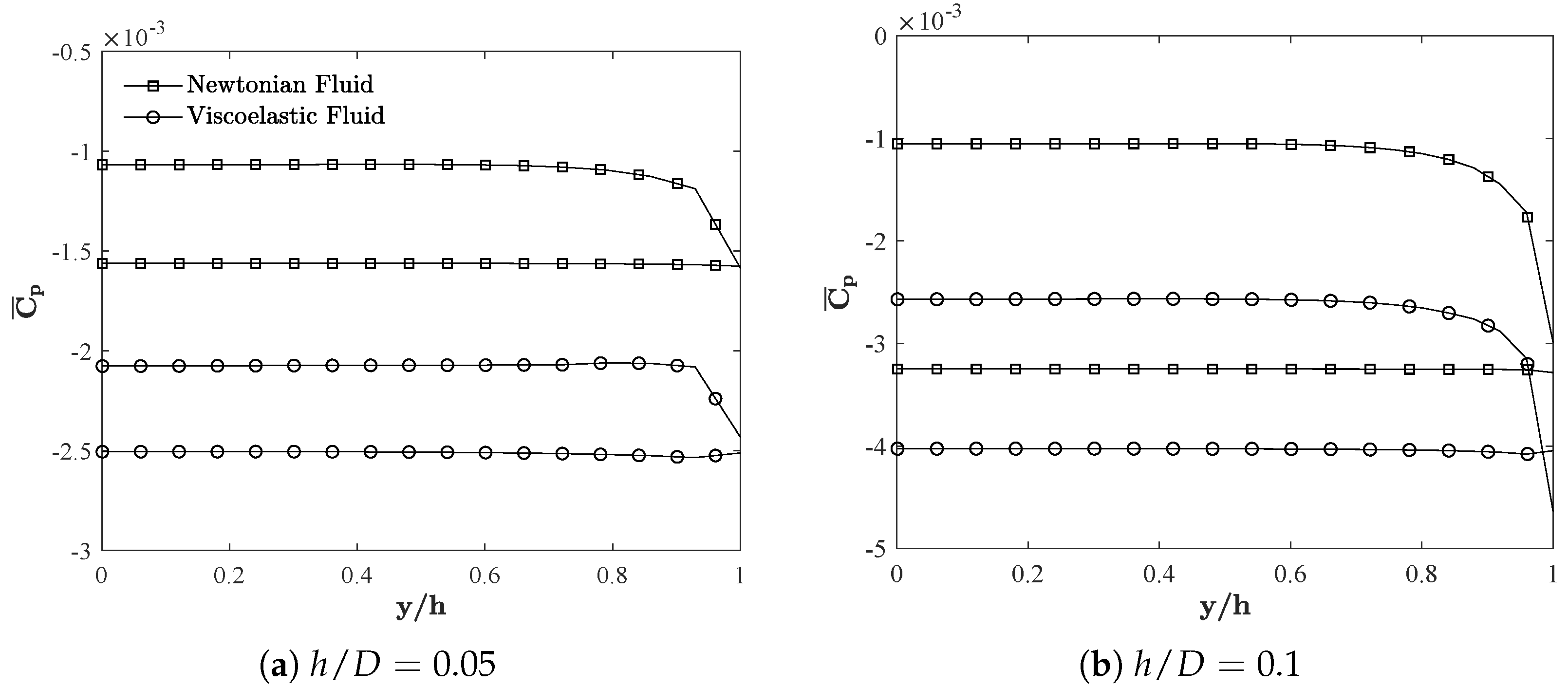
The distribution of mean pressure coefficient () was examined in Figure 8 for both roughness heights. The profiles were drawn along the wall for downstream of the roughness elements. For the Newtonian fluid, the pressure rose abruptly after in the case of , while the sudden increase in pressure for occurred at . These locations roughly coincided with the centre of the recirculation bubble behind the roughness element. This was in good agreement with Leonardi et al. (2003) [17] and Hemmati et al. (2019) [18], who stated that the flow starts experiencing adverse pressure gradients downstream of the centre of the recirculation bubble. In the case of viscoelastic fluid, however, the initial increase in the pressure was noted near the stagnation point. Farther downstream, pressure reduced for the smaller bar height (), while it stabilized for . For the latter, pressure dropped as the flow progressed downstream. This suggests that high pressure gradients formed due to the increased near-wall flow interactions for Newtonian flow diffused quickly in the case of viscoelastic flow. Thus, it facilitated the flow recovery towards an equilibrium state faster.
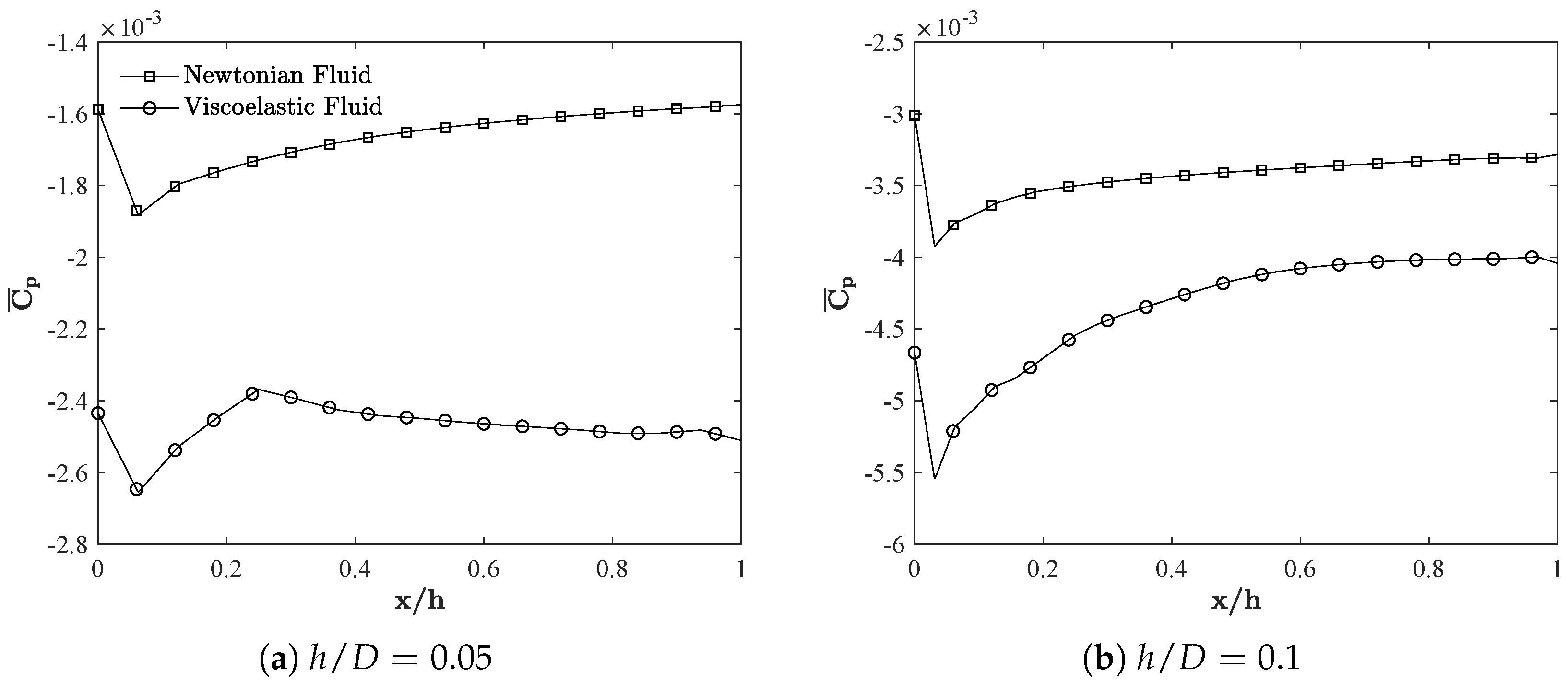
Profiles of mean pressure coefficient on the upstream and downstream faces of the roughness element are shown in Figure 9. Here, it was apparent that larger roughness elements produced greater pressure loss with Newtonian fluid. This observation was consistent with the findings of Liu et al. (2019) [52] on Newtonian flow over an array of periodic roughness elements. Similarities were observed with viscoelastic flow, where pressure losses were higher for a larger element compared to a smaller element. Furthermore, pressure on surfaces of the roughness element was significantly lower for the Viscoelastic fluid compared to the Newtonian fluid for both bar heights. This hinted at a reduction in generated drag on the perturbation surfaces due to Viscoelastic effects.
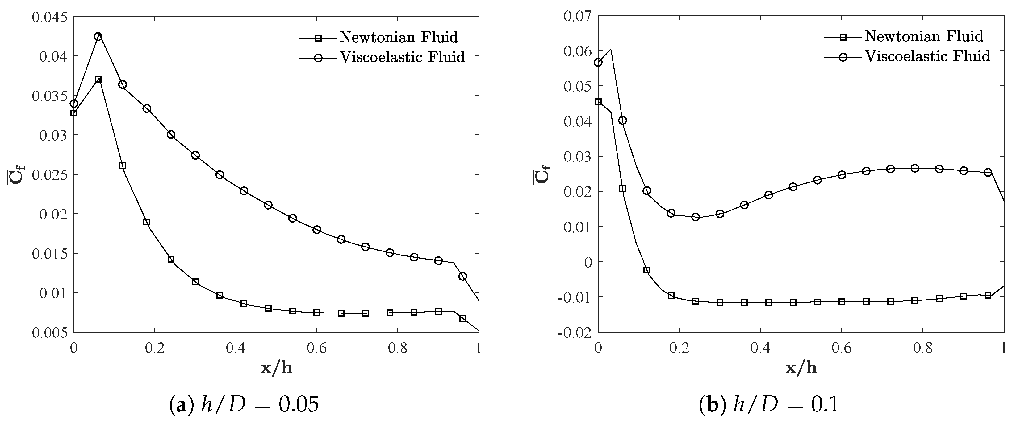
The distribution of pressure and skin friction on the top surface of the perturbation is shown in Figure 10 and Figure 11. The trend for the pressure profiles followed an initial drop for all cases, which was followed by a gradual increase. These were associated with the flow separation on the top surface of the roughness element. Location of the initial collapse in pressure suggested a strong average pressure gradient forming by flow separation on the leading edge of the roughness element. This suggested a local flow acceleration, which was evident by the sharp initial rise in skin friction from Figure 11. As the flow progressed downstream, there was a sudden increase in pressure near the wall (see Figure 8) along with a drop in skin friction. Thus, the effect of viscosity became dominant in the response and recovery on mean flow. Furthermore, pressure losses were higher for the larger roughness element in both fluids. For the viscoelastic fluid, these were significantly lower than those observed for the Newtonian fluid. In the case of the latter, the pressure coefficient increased again up to for both element heights. The skin friction (Figure 11) was initially large, but then it experienced a rapid reduction to an equilibrium constant value for both bar heights, reflecting the acceleration of the flow near the roughness leading edge. Negative skin friction occurred for , indicating the existence of a recirculating region on top of the roughness element.
For viscoelastic fluid, the initial drop in pressure was followed by a gradual increase towards relatively constant values near the downstream edge of the roughness element. The pressure losses for the larger bar were higher compared to the smaller bar, following the trend of the Newtonian fluid. The skin friction for dropped gradually up to before an abrupt drop was observed near the downstream face of the roughness. For the larger bar element (), it increased to achieve a constant value suggesting that the flow was accelerating near the downstream edge. This may be due to the fact that, as mentioned before, the larger bar element extended outside the boundary layer, whereas the smaller bar height was submerged in the boundary layer. The magnitude of the skin friction was higher in the Viscoelastic flow, which hinted at a higher contribution of viscous stresses to the local drag induced on the roughness. This was while the contribution of pressure drag due to the larger pressure losses on the front and back surfaces of the roughness element was lowered. Thus, the overall induced drag on the roughness element was reduced with viscoelastic fluid, leading to a smaller recirculation region and a faster recovery.
4. Conclusions
The implications of viscoelastic fluid on the response and recovery of mean flow over two roughness element heights ( and ) were examined using Direct Numerical Simulations at . For viscoelastic simulations, a Finitely Extensible Non-linear Elastic-Peterlin (FENE-P) rheological model was considered with the rheological parameters corresponding to a high-molecular weight polymer additive of 160 ppm concentration. The response behaviour was evaluated by studying the mean wake features behind the roughness element. The streamlines for viscoelastic fluid showed a shorter recirculating region for both bar heights compared to that of the Newtonian fluid. The lateral width of the recirculating bubble did not extend above the height of the roughness element contrary to the Newtonian flow. The reattachment length was significantly reduced, e.g., ∼73% for and ∼50% for . The larger roughness element created a larger contraction in the flow, which was noticeable from the Newtonian fluid. Due to the high suppression of velocity gradients in the vicinity of the roughness element, compared to Newtonian fluid, the effects of pressure gradients were not significant in viscoelastic fluid, even for the larger roughness element. Thus, it led to a shorter reattachment length. Looking at the velocity field, the progression of velocity was slower for the smaller bar height compared to the larger element in Newtonian flow. For viscoelastic fluid, the velocity near the centre of the pipe appeared to have recovered close to the fully developed profile for the smaller roughness element, while a full recovery was observed for the larger element with only slight variations. The mean flow recovery for the Newtonian fluid was slower than that of viscoelastic flow. This was consistent for both bar heights with ∼71% faster recovery of viscoelastic flow for compared to ∼70% for . This accelerated recovery of mean flow was attributed to the shear-thinning effects due to the reduced solution viscosity by the addition of polymeric additives.
The distribution of pressure on the pipe wall downstream of the roughness element coincided with the centre of the separation region, after which the flow started experiencing adverse pressure gradients. The pressure for viscoelastic fluid appeared to subside to an equilibrium state faster than the Newtonian flow. The distribution of pressure on the front and back surfaces of the roughness element indicated a larger pressure loss by the viscoelastic fluid compared to the Newtonian fluid. Furthermore, pressure losses by a larger element were greater than that of the smaller element with viscoelastic flow, an observation similar to that of Newtonian flows. This suggested that the roughness height is a prominent parameter in perturbed flows independent of Newtonian or viscoelastic characteristics of the flow. The contribution of viscous stresses to the overall local drag in viscoelastic flow was higher on the top surface of the roughness element, while that of pressure drag was lowered due to large pressure losses. Thus, the overall localized drag on the roughness element was greatly reduced for viscoelastic fluid, which led to a faster recovery.
Author Contributions
Conceptualization, methodology, formal analysis, investigation, writing—original draft preparation, S.G.; resources, writing—review and editing, supervision, project administration, funding acquisition, A.H. Both authors have read and agreed to the published version of the manuscript.
Funding
This work received financial support from Alberta Innovates and the Canada First Research Excellence and Alberta Innovates.
Data Availability Statement
The data presented in this study are available on request from the corresponding author.
Acknowledgments
Computational resources from Compute Canada were used for the simulations.
Conflicts of Interest
The authors declare no conflict of interest.
References
- Hart, A. A review of technologies for transporting heavy crude oil and bitumen via pipelines. J. Pet. Explor. Prod. Technol. 2014, 4, 327–336. [Google Scholar] [CrossRef] [Green Version]
- Abdul-Hadi, A.A.; Khadom, A.A. Studying the effect of some surfactants on drag reduction of crude oil flow. Chin. J. Eng. 2013, 2013, 1–6. [Google Scholar] [CrossRef] [Green Version]
- White, C.M.; Mungal, M.G. Mechanics and prediction of turbulent drag reduction with polymer additives. Annu. Rev. Fluid Mech. 2008, 40, 235–256. [Google Scholar] [CrossRef]
- White, C.M.; Somandepalli, V.S.R.; Mungal, M.G. The turbulence structure of drag-reduced boundary layer flow. Exp. Fluids 2004, 36, 62–69. [Google Scholar] [CrossRef]
- Toms, B.A. Some observations on the flow of linear polymer solutions through straight tubes at large Reynolds numbers. Proc. Inf. Cong. Rheol. 1948, 1948, 135. [Google Scholar]
- Hanks, R.W. Fluid Dynamics (Chemical Engineering); Elsevier: Amsterdam, The Netherlands, 2003. [Google Scholar]
- Burger, E.D.; Munk, W.R.; Wahl, H.A. Flow increase in the Trans Alaska Pipeline through use of a polymeric drag-reducing additive. J. Pet. Technol. 1982, 34, 377–386. [Google Scholar] [CrossRef]
- Takeuchi, H. Demonstration test of energy conservation of central air conditioning system at the Sapporo City Office Building—Reduction of pump power by flow drag reduction using surfactant. Synth. Engl. Ed. 2012, 4, 136–143. [Google Scholar]
- Sellin, R.H.J. Drag reduction in sewers: First results from a permanent installation. J. Hydraul. Res. 1978, 16, 357–371. [Google Scholar] [CrossRef]
- Fabula, A.G. Fire-Fighting Benefits of Polymeric Friction Reduction. J. Basic Eng. 1971, 93, 453–455. [Google Scholar] [CrossRef]
- Verma, S.; Hemmati, A. Performance of Overset Mesh in Modeling the Wake of Sharp-Edge Bodies. Computation 2020, 8, 66. [Google Scholar] [CrossRef]
- Smits, A.J.; Young, S.T.B.; Bradshaw, P. The effect of short regions of high surface curvature on turbulent boundary layers. J. Fluid Mech. 1979, 94, 209–242. [Google Scholar] [CrossRef]
- Durst, F.; Wang, A.B. Experimental and numerical investigations of the axisymmetric, turbulent pipe flow over a wall-mounted thin obstacle. In Proceedings of the 7th Symposium on Turbulent Shear Flows, Stanford, CA, USA, 21–23 August 1989; Volume 1, pp. 4–10. [Google Scholar]
- Dimaczek, G.; Tropea, C.; Wang, A.B. Turbulent flow over two-dimensional, surface-mounted obstacles: Plane and axisymmetric geometries. In Advances in Turbulence 2; Springer: Berlin/Heidelberg, Germany, 1989; pp. 114–121. [Google Scholar]
- Jiménez, J. Turbulent flows over rough walls. Annu. Rev. Fluid Mech. 2004, 36, 173–196. [Google Scholar] [CrossRef]
- Smits, A.; Ding, L.; Van Buren, T. Flow over a square bar roughness. In Proceedings of the 11th International Symposium on Turbulence and Shear Flow Phenomena, Southampton, UK, 30 July–2 August 2019. [Google Scholar]
- Leonardi, S.; Orlandi, P.; Smalley, R.J.; Djenidi, L.; Antonia, R.A. Direct numerical simulations of turbulent channel flow with transverse square bars on one wall. J. Fluid Mech. 2003, 491, 229. [Google Scholar] [CrossRef] [Green Version]
- Hemmati, A.; Wood, D.H.; Martinuzzi, R.J. Wake dynamics and surface pressure variations on two-dimensional normal flat plates. AIP Adv. 2019, 9, 045209. [Google Scholar] [CrossRef] [Green Version]
- Goswami, S.; Hemmati, A. Response of turbulent pipeflow to multiple square bar roughness elements at high Reynolds number. Phys. Fluids 2020, 32, 075110. [Google Scholar] [CrossRef]
- Goswami, S.; Hemmati, A. Evolution of turbulent pipe flow recovery over a square bar roughness element at a range of Reynolds numbers. Phys. Fluids 2021, 33, 035113. [Google Scholar] [CrossRef]
- Favero, J.L.; Secchi, A.R.; Cardozo, N.S.M.; Jasak, H. Viscoelastic flow analysis using the software OpenFOAM and differential constitutive equations. J. Non-Newton. Fluid Mech. 2010, 165, 1625–1636. [Google Scholar] [CrossRef]
- Tsukahara, T.; Kawase, T.; Kawaguchi, Y. DNS of viscoelastic turbulent channel flow with rectangular orifice at low Reynolds number. Int. J. Heat Fluid Flow 2011, 32, 529–538. [Google Scholar] [CrossRef] [Green Version]
- Holmes, L.; Favero, J.; Osswald, T. Numerical simulation of three-dimensional viscoelastic planar contraction flow using the software OpenFOAM. Comput. Chem. Eng. 2012, 37, 64–73. [Google Scholar] [CrossRef]
- Azaiez, J.; Guénette, R.; Ait-Kadi, A. Numerical simulation of viscoelastic flows through a planar contraction. J. Non-Newton. Fluid Mech. 1996, 62, 253–277. [Google Scholar] [CrossRef]
- Dubief, Y.; Terrapon, V.E.; Soria, J. On the mechanism of elasto-inertial turbulence. Phys. Fluids 2013, 25, 110817. [Google Scholar] [CrossRef] [Green Version]
- Resende, P.R.; Pinho, F.T.; Younis, B.A.; Kim, K.; Sureshkumar, R. Development of a Low-Reynolds-number k-ω Model for FENE-P Fluids. Flow, Turbul. Combust. 2013, 90, 69–94. [Google Scholar] [CrossRef]
- Resende, P.R.; Kim, K.; Younis, B.A.; Sureshkumar, R.; Pinho, F.T. A FENE-P k-ε turbulence model for low and intermediate regimes of polymer-induced drag reduction. J. Non-Newton. Fluid Mech. 2011, 166, 639–660. [Google Scholar] [CrossRef]
- Tsukahara, T.; Motozawa, M.; Tsurumi, D.; Kawaguchi, Y. PIV and DNS analyses of viscoelastic turbulent flows behind a rectangular orifice. Int. J. Heat Fluid Flow 2013, 41, 66–79. [Google Scholar] [CrossRef]
- Shaban, S.; Azad, M.; Trivedi, J.; Ghaemi, S. Investigation of near-wall turbulence in relation to polymer rheology. Phys. Fluids 2018, 30, 125111. [Google Scholar] [CrossRef]
- Samanta, D.; Dubief, Y.; Holzner, M.; Schäfer, C.; Morozov, A.N.; Wagner, C.; Hof, B. Elasto-inertial turbulence. Proc. Natl. Acad. Sci. USA 2013, 110, 10557–10562. [Google Scholar] [CrossRef] [PubMed] [Green Version]
- Quinzani, L.M.; Armstrong, R.C.; Brown, R.A. Birefringence and laser-Doppler velocimetry (LDV) studies of viscoelastic flow through a planar contraction. J. Non-Newton. Fluid Mech. 1994, 52, 1–36. [Google Scholar] [CrossRef]
- Oldroyd, J.G. On the formulation of rheological equations of state. Proc. R. Soc. Lond. Ser. Math. Phys. Sci. 1950, 200, 523–541. [Google Scholar]
- Giesekus, H. A simple constitutive equation for polymer fluids based on the concept of deformation-dependent tensorial mobility. J. Non-Newton. Fluid Mech. 1982, 11, 69–109. [Google Scholar] [CrossRef]
- Phan-Thien, N. A nonlinear network viscoelastic model. J. Rheol. 1978, 22, 259–283. [Google Scholar] [CrossRef]
- Bird, R.B.; Armstrong, R.C.; Hassager, O. Dynamics of Polymeric Liquids: Fluid Mechanics, 2nd ed.; John Wiley and Sons: New York, NY, USA, 1987; Volume 1. [Google Scholar]
- Macosko, C.W. Rheology: Principles, Measurements, and Applications; VCH Publishers Inc.: New York, NY, USA, 1994. [Google Scholar]
- Sureshkumar, R.; Beris, A.N.; Handler, R.A. Direct numerical simulation of the turbulent channel flow of a polymer solution. Phys. Fluids 1997, 9, 743–755. [Google Scholar] [CrossRef]
- Warner, H.R., Jr. Kinetic theory and rheology of dilute suspensions of finitely extendible dumbbells. Ind. Eng. Chem. Fundam. 1972, 11, 379–387. [Google Scholar] [CrossRef]
- Rothstein, J.P.; McKinley, G.H. The axisymmetric contraction–expansion: The role of extensional rheology on vortex growth dynamics and the enhanced pressure drop. J. Non-Newton. Fluid Mech. 2001, 98, 33–63. [Google Scholar] [CrossRef]
- Poole, R.J.; Escudier, M.P. Turbulent flow of non-Newtonian liquids over a backward-facing step: Part II, Viscoelastic and shear-thinning liquids. J. Non-Newton. Fluid Mech. 2003, 109, 193–230. [Google Scholar] [CrossRef]
- Oliveira, P.J. Asymmetric flows of viscoelastic fluids in symmetric planar expansion geometries. J. Non-Newton. Fluid Mech. 2003, 114, 33–63. [Google Scholar] [CrossRef] [Green Version]
- Poole, R.J.; Escudier, M.P.; Afonso, A.; Pinho, F.T. Laminar flow of a viscoelastic shear-thinning liquid over a backward-facing step preceded by a gradual contraction. Phys. Fluids 2007, 19, 093101. [Google Scholar] [CrossRef] [Green Version]
- Xiong, Y.L.; Bruneau, C.H.; Kellay, H. A numerical study of two dimensional flows past a bluff body for dilute polymer solutions. J. Non-Newton. Fluid Mech. 2013, 196, 8–26. [Google Scholar] [CrossRef] [Green Version]
- Tsukahara, T.; Tanabe, M.; Kawaguchi, Y. Effect of fluid viscoelasticity on turbulence and large-scale vortices behind wall-mounted plates. Adv. Mech. Eng. 2014, 6, 823138. [Google Scholar] [CrossRef]
- Tsukahara, T.; Kawase, T.; Kawaguchi, Y. DNS on turbulent heat transfer of viscoelastic fluid flow in a plane channel with transverse rectangular orifices. Prog. Comput. Fluid Dyn. Int. J. 2013, 13, 212–223. [Google Scholar] [CrossRef]
- Yamagata, T.; Ito, A.; Sato, Y.; Fujisawa, N. Experimental and numerical studies on mass transfer characteristics behind an orifice in a circular pipe for application to pipe-wall thinning. Exp. Therm. Fluid Sci. 2014, 52, 239–247. [Google Scholar] [CrossRef]
- Hemmati, A.; Wood, D.H.; Martinuzzi, R.J. On simulating the flow past a normal thin flat plate. J. Wind. Eng. Ind. Aerodyn. 2018, 174, 170–187. [Google Scholar] [CrossRef]
- Ashrafian, A.; Andersson, H.I.; Manhart, M. DNS of turbulent flow in a rod-roughened channel. Int. J. Heat Fluid Flow 2004, 25, 373–383. [Google Scholar] [CrossRef]
- McKeon, B.J.; Swanson, C.J.; Zagarola, M.V.; Donnelly, R.J.; Smits, A.J. Friction factors for smooth pipe flow. J. Fluid Mech. 2004, 511, 41–44. [Google Scholar] [CrossRef] [Green Version]
- Jasak, H.; Jemcov, A.; Tukovic, Z. OpenFOAM: A C++ library for complex physics simulations. In International Workshop on Coupled Methods in Numerical Dynamics; IUC Dubrovnik Croatia: Dubrovnik, Croatia, 2007; Volume 1000, pp. 1–20. [Google Scholar]
- Hultmark, M.; Vallikivi, M.; Bailey, S.C.C.; Smits, A.J. Turbulent pipe flow at extreme Reynolds numbers. Phys. Rev. Lett. 2012, 108, 094501. [Google Scholar] [CrossRef] [Green Version]
- Liu, Y.; Li, J.; Smits, A.J. Roughness effects in laminar channel flow. J. Fluid Mech. 2019, 876, 1129–1145. [Google Scholar] [CrossRef]
Figure 1.
Comparison of the mean axial velocity profiles () with the experimental study of Shaban et al. (2018) [29].
Figure 1.
Comparison of the mean axial velocity profiles () with the experimental study of Shaban et al. (2018) [29].

Figure 2.
Cross-sectional schematics of the computational domain (not to scale).

Figure 3.
The spatial grid distribution with a magnified box around the bar roughness element.

Figure 4.
Streamline plot of the (a) Newtonian fluid and (b) viscoelastic fluid flow past a roughness element of bar height .
Figure 4.
Streamline plot of the (a) Newtonian fluid and (b) viscoelastic fluid flow past a roughness element of bar height .

Figure 5.
Streamline plot of the (a) Newtonian fluid and (b) viscoelastic fluid flow past a roughness element of bar height .
Figure 5.
Streamline plot of the (a) Newtonian fluid and (b) viscoelastic fluid flow past a roughness element of bar height .

Figure 6.
Mean axial velocity profiles () at different axial locations ( and 100) for .

Figure 7.
Mean axial velocity profiles () at different axial locations ( and 100) for .

Figure 8.
Mean pressure coefficient profile () on the pipe wall behind both bar heights at 0–50.

Figure 9.
Mean pressure coefficient profile () along the roughness element upstream and downstream surfaces.
Figure 9.
Mean pressure coefficient profile () along the roughness element upstream and downstream surfaces.

Figure 10.
Mean pressure coefficient profile () along the top surface of the roughness element.

Figure 11.
Wall shear stress distribution () along the top surface of the roughness elements.


Table 1.
Grid resolution, , for the current DNS study.
| Case | 1 | 2 | 5 | 8 | |
|---|---|---|---|---|---|
| Current Case | |||||
| Hemmati et al. (2018) [47] | |||||
| Ashrafian et al. (2004) [48] | ≈3.2 | − | − | − | |
| Dubief et al. (2013) [25] | ≈2.3 | − | − | − |
Table 2.
Parameter space for the current study.
| Parameter | Value |
|---|---|
| Extensibility of the polymer, | 200 |
| Ratio of solvent to zero-shear viscosity, | |
| Polymer relations time, (s) | |
| Reynolds number, | 5000 |
| Frictional Reynolds number, | 384 |
Table 3.
The mean recirculation length () for Newtonian and non-Newtonian flows over roughness elements.
Table 3.
The mean recirculation length () for Newtonian and non-Newtonian flows over roughness elements.
| Study | |||
|---|---|---|---|
| Newtonian | − | ||
| Viscoelastic | 73 | ||
| Newtonian | − | ||
| Viscoelastic |
Table 4.
The recovery locations compared between Newtonian and viscoelastic flows, for both roughness heights.
Table 4.
The recovery locations compared between Newtonian and viscoelastic flows, for both roughness heights.
| Study | |||
|---|---|---|---|
| Newtonian | 350 | − | |
| Viscoelastic | 100 | 71 | |
| Newtonian | 200 | − | |
| Viscoelastic | 60 | 70 |
Publisher’s Note: MDPI stays neutral with regard to jurisdictional claims in published maps and institutional affiliations. |
© 2021 by the authors. Licensee MDPI, Basel, Switzerland. This article is an open access article distributed under the terms and conditions of the Creative Commons Attribution (CC BY) license (https://creativecommons.org/licenses/by/4.0/).
Share and Cite
MDPI and ACS Style
Goswami, S.; Hemmati, A. Response of Viscoelastic Turbulent Pipeflow Past Square Bar Roughness: The Effect on Mean Flow. Computation 2021, 9, 85. https://0-doi-org.brum.beds.ac.uk/10.3390/computation9080085
AMA Style
Goswami S, Hemmati A. Response of Viscoelastic Turbulent Pipeflow Past Square Bar Roughness: The Effect on Mean Flow. Computation. 2021; 9(8):85. https://0-doi-org.brum.beds.ac.uk/10.3390/computation9080085
Chicago/Turabian StyleGoswami, Shubham, and Arman Hemmati. 2021. "Response of Viscoelastic Turbulent Pipeflow Past Square Bar Roughness: The Effect on Mean Flow" Computation 9, no. 8: 85. https://0-doi-org.brum.beds.ac.uk/10.3390/computation9080085
Note that from the first issue of 2016, this journal uses article numbers instead of page numbers. See further details here.