Parameter Estimation of Partially Observed Turbulent Systems Using Conditional Gaussian Path-Wise Sampler

Abstract

Parameter estimation of complex nonlinear turbulent dynamical systems using only partially observed time series is a challenging topic. The nonlinearity and partial observations often impede using closed analytic formulae to recover the model parameters. In this paper, an exact path-wise sampling method is developed, which is incorporated into a Bayesian Markov chain Monte Carlo (MCMC) algorithm in light of data augmentation to efficiently estimate the parameters in a rich class of nonlinear and non-Gaussian turbulent systems using partial observations. This path-wise sampling method exploits closed analytic formulae to sample the trajectories of the unobserved variables, which avoid the numerical errors in the general sampling approaches and significantly increase the overall parameter estimation efficiency. The unknown parameters and the missing trajectories are estimated in an alternating fashion in an adaptive MCMC iteration algorithm with rapid convergence. It is shown based on the noisy Lorenz 63 model and a stochastically coupled FitzHugh–Nagumo model that the new algorithm is very skillful in estimating the parameters in highly nonlinear turbulent models. The model with the estimated parameters succeeds in recovering the nonlinear and non-Gaussian features of the truth, including capturing the intermittency and extreme events, in both test examples.

1. Introduction

Complex nonlinear turbulent dynamical systems are ubiquitous in many areas, including geophysics, engineering, material science, and neural science [1,2,3,4]. Estimating the model parameters is a crucial prerequisite for data assimilation, uncertainty quantification, and prediction [5,6]. However, parameter estimation of these nonlinear systems is a big challenge for the following reasons. First, these systems often have strong non-Gaussian features [7,8]. The intermittent instability, the extreme events, and the associated non-Gaussian probability density functions (PDFs) with significant skewness or fat tails can easily break the conditions that are required in many existing parameter estimation algorithms designed for more stabilized or laminar systems. Second, the dimension of many complex turbulent systems is quite large [9,10,11,12], which requires the development of efficient parameter estimation algorithms that can overcome the curse of dimensionality [13,14]. Finally, one of the key features of many turbulent dynamical systems is the availability of only the partial observations [15,16,17]. Despite the lack of observational data, the unresolved variables nevertheless play a crucial role in transferring energy with the observed or resolved variables in a highly nonlinear way [18,19]. These unobserved variables are also able to trigger various non-Gaussian phenomena including extreme events in both the resolved and unresolved scales [6,20]. Unfortunately, many desirable mathematical formulations for the parameter estimation algorithms in the presence of full observations are no longer applicable to the partially observed turbulent systems, which leads to a fundamental difficulty in recovering the model parameters.

Several parameter estimation algorithms have been developed for turbulent systems. One simple and frequently adopted parameter estimation approach is based on computing maximum a posteriori or maximum likelihood estimates [21,22,23]. Another commonly used method is the expectation–maximization algorithms [24,25,26,27], where the target energy function is evaluated recursively. Other parameter estimation algorithms based on specific cost functions are also routinely seen depending on the applications [28,29,30,31,32,33].

Among all the parameter estimation algorithms, the Bayesian approaches are widely applied in many practical problems. One of the commonly used Bayesian techniques is the Markov chain Monte Carlo (MCMC) method [34,35,36], which samples the so-called posterior distribution of the parameters conditioned on the given observations. In the situation with partial observations, data augmentation [37] is often incorporated into the MCMC algorithm [38,39]. Then, the MCMC algorithm is applied to sample the parameters and the unobserved trajectories in an alternating fashion. The main challenge in simultaneously sampling the parameters and the hidden trajectories comes from the high-dimensional representation of the latter even in the presence of a low-dimensional dynamical system. In fact, the degree of freedom needed to characterize a trajectory equals the total time instants. Even with the time discretization approximation, a large number of the temporal points are required to fully represent a trajectory. This raises a challenge in the sampling procedure. To this end, several innovative updating strategies have been developed in the context of multivariate diffusion models [40,41,42,43,44,45,46,47,48]. While these methods are designed for general nonlinear models, specific methods can be developed in light of the model structures, which then have the potential to further facilitate sampling and parameter estimation.

The focus of this paper is on a rich class of complex nonlinear turbulent systems [49,50,51]. This rich class of the complex turbulent models is highly nonlinear and non-Gaussian but certain conditional distributions are Gaussian. These systems have wide applications in modeling and predicting many important phenomena in geophysics [52,53,54], climate science [55,56,57], and neural science [58,59]. Specific examples include the Lorenz models (Lorenz 63, 84, and two-layered 96 models), Boussinesq equations with noise, and a variety of the stochastically coupled FitzHugh–Nagumo model. Despite being highly nonlinear, this paper aims at showing that the conditional Gaussian structure can be explored to the development of an efficient path-wise sampling strategy, which is then incorporated into an MCMC algorithm to advance the parameter estimation using only partial observations. The advantage of such a path-wise sampling algorithm is that the sampled trajectories can be written using closed analytic formulae in light of the conditional Gaussian statistics, which are not achievable for general nonlinear systems. Therefore, the new parameter estimation algorithm is extremely efficient and avoids potential numerical errors. It also has the potential to be applied in high-dimensional systems due to its analytically solvable characteristics.

The rest of the paper is organized as follows. The rich class of complex nonlinear turbulent systems with conditional statistics is introduced in Section 2. Section 3 focuses on the development of the sampling and parameter estimation algorithm. Section 4 includes the numerical test experiments. The paper is concluded in Section 5.

2. The Nonlinear Turbulent Models with Conditional Gaussian Statistics

The general framework of the nonlinear and non-Gaussian turbulent dynamical models considered in this paper is as follows [49,51]:

$$\begin{array}{cc}\hfill \mathrm{d}\mathbf{X}\left(t\right)& =\left[{\mathbf{A}}_{\mathbf{0}}(\mathbf{X},t)+{\mathbf{A}}_{\mathbf{1}}(\mathbf{X},t)\mathbf{Y}\left(t\right)\right]\mathrm{d}t+\mathbf{B}(\mathbf{X},t)\mathrm{d}{\mathbf{W}}_{\mathbf{X}}\left(t\right),\hfill \end{array}$$

(1a)

$$\begin{array}{cc}\hfill \mathrm{d}\mathbf{Y}\left(t\right)& =\left[{\mathbf{a}}_{\mathbf{0}}(\mathbf{X},t)+{\mathbf{a}}_{\mathbf{1}}(\mathbf{X},t)\mathbf{Y}\left(t\right)\right]\mathrm{d}t+\mathbf{b}(\mathbf{X},t)\mathrm{d}{\mathbf{W}}_{\mathbf{Y}}\left(t\right).\hfill \end{array}$$

(1b)

In the coupled system (1a) and (1b), the state variables are $\mathbf{X}$ and $\mathbf{Y}$, which are both column vectors representing the multi-dimensional states. On the right-hand side of (1a) and (1b), ${\mathbf{A}}_0$, and ${\mathbf{a}}_0$ are column vectors while ${\mathbf{A}}_{\mathbf{1}}$, ${\mathbf{a}}_{\mathbf{1}}$, $\mathbf{b}$, and $\mathbf{B}$ are matrices. All of them can depend nonlinearly on the state variables $\mathbf{X}$ and time t but not the state variable $\mathbf{Y}$. The vectors ${\mathbf{W}}_{\mathbf{1}}$ and ${\mathbf{W}}_{\mathbf{2}}$ are independent white noise sources. For complex nonlinear turbulent systems with partial observations, $\mathbf{X}$ can be regarded as the collection of the observed variables while $\mathbf{Y}$ contains the variables that are not directly observed.

Because of the strong nonlinearity in ${\mathbf{A}}_0(\mathbf{X},t)$, ${\mathbf{A}}_1(\mathbf{X},t)$, ${\mathbf{a}}_0(\mathbf{X},t)$ and ${\mathbf{a}}_0(\mathbf{X},t)$ and their coupling with $\mathbf{Y}$, its interaction with the white noise can easily induce non-Gaussian statistics for both the marginal and the joint distributions of the coupled system (1a) and (1b). Extreme events, intermittency, and complex nonlinear interactions between different variables all appear in such systems. Despite being highly nonlinear and non-Gaussian, the system in (1a) and (1b) has a desirable analytic feature. That is, conditioned on a given realization of $\mathbf{X}\left(s\right)$ for $s\le t$, the distribution of $\mathbf{Y}\left(t\right)$ is Gaussian. Therefore, the coupled system is called the conditional Gaussian nonlinear system.

The conditional Gaussian nonlinear modeling framework (1a) and (1b) includes many physics-constrained nonlinear stochastic models, large-scale dynamical models in turbulence, fluids, and geophysical flows, as well as stochastically coupled reaction-diffusion models in neuroscience and ecology. A gallery of examples of conditional Gaussian systems in engineering, neuroscience, ecology, fluids, and geophysical flows can be found in [49].

3. The Parameter Estimation Algorithm

3.1. The General Bayesian MCMC Parameter Estimation Framework with Partial Observations

Denote $\theta$ as the collection of the parameters to be estimated in the coupled system (1a) and (1b), where $\theta$ can appear in ${\mathbf{A}}_0$, ${\mathbf{A}}_1$, ${\mathbf{a}}_0$, ${\mathbf{a}}_1$, $\mathbf{b}$, and $\mathbf{B}$. Assume ${\mathbf{X}}^{obs}$ is the given trajectory of the state variable $\mathbf{X}$ in (1a) and (1b) within the time interval $[0,T]$. The goal of parameter estimation in the Bayesian framework is to find the conditional distribution, which is also known as the posterior distribution,

$$p(\theta |{\mathbf{X}}^{obs})\propto p\left(\theta \right)p({\mathbf{X}}^{obs}|\theta ).$$

(2)

In (2), $p\left(\theta \right)$ is the prior distribution, which is based on the empirical knowledge of choosing the parameter $\theta$, while $p({\mathbf{X}}^{obs}|\theta )$ is the likelihood function. Since the nonlinear system (1a) and (1b) is only partially observed, the closed analytic formula of solving (2) is in general not available. One strategy to solve (2) is to apply the data augmentation technique [37], which augments the target state space variables from $\theta$ to $(\theta ,{\mathbf{Y}}^{hidden})$. Here, ${\mathbf{Y}}^{hidden}$ is the trajectories of the unobserved variable $\mathbf{Y}$. In such a way, the Bayesian framework in (2) is modified to

$$\begin{array}{cc}\hfill p(\theta ,{\mathbf{Y}}^{hidden}|{\mathbf{X}}^{obs})& \propto p(\theta ,{\mathbf{Y}}^{hidden},{\mathbf{X}}^{obs})\hfill \end{array}$$

(3a)

$$\begin{array}{cc}\hfill & =p\left(\theta \right)p({\mathbf{X}}^{obs},{\mathbf{Y}}^{hidden}|\theta )\hfill \end{array}$$

(3b)

$$\begin{array}{cc}\hfill & =p\left(\theta \right)p({\mathbf{Y}}^{hidden}|\theta )p({\mathbf{X}}^{obs}|{\mathbf{Y}}^{hidden},\theta ).\hfill \end{array}$$

(3c)

It is clear from (3a)–(3c) that, if $p(\theta ,{\mathbf{Y}}^{hidden}|{\mathbf{X}}^{obs})$ is solved, then $p(\theta |{\mathbf{X}}^{obs})$ can be reached by marginalizing over the auxiliary variable ${\mathbf{Y}}^{hidden}$. Therefore, the goal here is to develop a suitable MCMC algorithm to compute the posterior distribution $p(\theta ,{\mathbf{Y}}^{hidden}|{\mathbf{X}}^{obs})$. In addition to the prior distribution $p\left(\theta \right)$, the other two components on the right-hand side of (3c) represent the probability of the sampled trajectory of the hidden variable given the parameters $p({\mathbf{Y}}^{hidden}|\theta )$ and the likelihood of the observed trajectory conditioned on both the sampled one and parameters $p({\mathbf{X}}^{obs}|{\mathbf{Y}}^{hidden},\theta )$.

Comparing with (2), the most significant improvement in (3a)–(3c) is the solvability of the likelihood function. In fact, if the unobserved trajectory ${\mathbf{Y}}^{hidden}$ is given, then a closed analytic formula of the likelihood $p({\mathbf{X}}^{obs}|{\mathbf{Y}}^{hidden},\theta )$ is available. Specifically, assume a time discretization of both the trajectories ${\mathbf{X}}^{obs}$ and ${\mathbf{Y}}^{hidden}$ denoted by

$$\begin{array}{cc}\hfill {\tilde{\mathbf{X}}}^{obs}& =({\tilde{\mathbf{X}}}_0^{obs},{\tilde{\mathbf{X}}}_1^{obs},\dots ,{\tilde{\mathbf{X}}}_n^{obs})\hfill \\ \hfill {\tilde{\mathbf{Y}}}^{hidden}& =({\tilde{\mathbf{Y}}}_0^{hidden},{\tilde{\mathbf{Y}}}_1^{hidden},\dots ,{\tilde{\mathbf{Y}}}_n^{hidden}),\hfill \end{array}$$

(4)

where ${\tilde{\mathbf{X}}}_i^{obs}={\mathbf{X}}^{obs}\left(t_i\right)$ and ${\tilde{\mathbf{Y}}}_i^{hidden}={\mathbf{Y}}^{hidden}\left(t_i\right)$. Here, the time interval is discretized with small subintervals $0=t_0<t_1<\dots ,<t_n=T$. The notation with tilde is for discrete approximation while that without tilde is for the original continuous time series. With such notations, the discrete version of the likelihood $p({\tilde{\mathbf{X}}}^{obs}|{\tilde{\mathbf{Y}}}^{hidden},\theta )$ can be written down explicitly:

$$p({\tilde{\mathbf{X}}}^{obs}|{\tilde{\mathbf{Y}}}^{hidden},\theta )=\prod _{i=1}^{n}p({\tilde{\mathbf{X}}}_i^{obs}|{\tilde{\mathbf{X}}}_{i-1}^{obs},{\tilde{\mathbf{Y}}}_{i-1}^{hidden},{\tilde{\mathbf{Y}}}_i^{hidden},\theta )$$

(5)

according to the Markov property. With a small time increment, each probability on the right-hand side of (5) can be computed using a Gaussian approximation based on a forward Euler scheme $p({\tilde{\mathbf{X}}}_i^{obs}|{\tilde{\mathbf{X}}}_{i-1}^{obs},{\tilde{\mathbf{Y}}}_{i-1}^{hidden},\theta )$. The product of these Gaussian distributions finishes the calculation of the likelihood.

On the other hand, the discrete approximation of $p({\mathbf{Y}}^{hidden}|\theta )$, i.e., $p({\tilde{\mathbf{Y}}}^{hidden}|\theta )$ can be solved via

$$p({\tilde{\mathbf{Y}}}^{hidden}|\theta )\propto L({\tilde{\mathbf{Y}}}^{hidden};\theta )=\prod _{i=1}^n{L}_i({\tilde{\mathbf{Y}}}_{[i-1,i]}^{hidden};\theta ),$$

(6)

where each $L_i({\tilde{\mathbf{Y}}}_{[i-1,i]}^{hidden};\theta )$ is given by

$$L_i({\tilde{\mathbf{Y}}}_{[i-1,i]}^{hidden};\theta )=exp\left({\int }_{i-1}^i\alpha ({\mathbf{Y}}_{scaled}^{hidden},\theta ,t)d{\mathbf{Y}}_{scaled}^{hidden}\right)exp\left(-\frac{1}{2}{\int }_{i-1}^i\alpha {({\mathbf{Y}}_{scaled}^{hidden},\theta ,t)}^{2}dt\right).$$

(7)

Formulas (6)–(7) basically follow the Girsanov formula [60]. In other words, the Equation (1b) is rescaled by

$$\mathrm{d}{\mathbf{Y}}_{scaled}^{hidden}=\alpha ({\mathbf{Y}}_{scaled}^{hidden},\theta ,t)\mathrm{d}t+\mathrm{d}{\mathbf{W}}_{\mathbf{Y}}\left(t\right),$$

(8)

where ${\mathbf{Y}}_{scaled}^{hidden}$ is the rescaled state variable of ${\mathbf{Y}}^{hidden}$ by dividing the noise coefficient $\mathbf{b}$ componentwise, assuming $\mathbf{b}$ is a diagonal matrix as in most of the applications. The reason to introduce the rescaled variable with an identity noise coefficient in (8) is the following. The probability $L({\tilde{\mathbf{Y}}}^{hidden};\theta )$ can be viewed as the Radon–Nikodym derivative of the measure induced by (1b) with respect to the Wiener measure scaled by the diffusion coefficient $\mathbf{b}$. Given that two such dominating measures (with different $\mathbf{b}$) are singular, a direct MCMC implementation will result in a reducible algorithm [38]. Note that the function $\alpha (·)$ depends on $\mathbf{X}$ as well. However, for the notation simplicity here, we drop such an explicit dependence.

It is also noticeable that the left-hand side is only proportional instead of equaling to the right-hand side in (6). Nevertheless, this is sufficient for the MCMC algorithm. The reason is that each step in the MCMC algorithm is to compute the ratio between the two $p({\tilde{\mathbf{Y}}}^{hidden}|\theta )$ in the previous and current steps. The pre-constants will cancel with each other in computing the ratio.

3.2. The Path-Wise Sampler of the Unobserved Trajectories

To apply the Bayesian MCMC parameter estimation algorithm, what remains is to develop an efficient path-wise sampler of the unobserved trajectory ${\mathbf{Y}}^{hidden}\left(t\right)$ given the parameters $\theta$, i.e., sampling from $p({\mathbf{Y}}^{hidden}|\theta )$ appearing in (3a)–(3c). In what follows, the goal is to develop an efficient sampling algorithm for the conditional distribution $p({\mathbf{Y}}^{hidden}|{\mathbf{X}}^{obs},\theta )$. Note that $p({\mathbf{Y}}^{hidden}|{\mathbf{X}}^{obs},\theta )$ is only a subset of $p({\mathbf{Y}}^{hidden}|\theta )$. Nevertheless, since the MCMC procedure also involves sampling from $p({\mathbf{X}}^{obs}|{\mathbf{Y}}^{hidden},\theta )$ in (3a)–(3c), the trajectories of ${\mathbf{Y}}^{hidden}$ sampled from $p({\mathbf{Y}}^{hidden}|{\mathbf{X}}^{obs},\theta )$ will lead to a higher probability for $p({\mathbf{X}}^{obs}|{\mathbf{Y}}^{hidden},\theta )$. This means that only those ${\mathbf{Y}}^{hidden}$ that are sampled from $p({\mathbf{Y}}^{hidden}|{\mathbf{X}}^{obs},\theta )$ will have a higher acceptance in the MCMC algorithm. Thus, sampling from $p({\mathbf{Y}}^{hidden}|{\mathbf{X}}^{obs},\theta )$ is a more efficient way than sampling from $p({\mathbf{Y}}^{hidden}|\theta )$. Notably, the path-wise sampler here exploits the closed analytic properties of the conditional statistics associated with the coupled nonlinear systems in (1a) and (1b). Data assimilation is utilized in the development of such a path-wise sampler. Throughout this subsection (Section 3.2), we use $p({\mathbf{Y}}^{hidden}|{\mathbf{X}}^{obs},\theta )$ to denote $p({\mathbf{Y}}^{hidden}|{\mathbf{X}}^{obs})$ since the parameters here are fixed.

As a prerequisite of the path-wise sampler, let us start with solving the conditional (or posterior) distribution $p({\mathbf{Y}}^{hidden}\left(t\right)|{\mathbf{X}}^{obs}\left(s\right),s\le t)$ at a fixed time instant t. This is also known as the filtering. For the conditional nonlinear Gaussian systems (1a) and (1b), the solution of the filtering can be written down with closed analytic formulae.

Theorem 1.

For the conditional Gaussian nonlinear systems (1a) and (1b), given one realization of ${\mathbf{X}}^{obs}\left(s\right)$ for $s\in [0,t]$, the conditional distribution $p({\mathbf{Y}}^{hidden}\left(t\right)|{\mathbf{X}}^{obs}\left(s\right),s\le t)\sim \mathcal{N}({\mu }_{\mathbf{f}}\left(t\right),{\mathbf{R}}_{\mathbf{f}}\left(t\right))$ is Gaussian. The conditional mean ${\mu }_{\mathbf{f}}$ and the conditional covariance ${\mathbf{R}}_{\mathbf{f}}$ are given by the following explicit formulae:

$$\begin{array}{cc}\hfill \mathrm{d}{\mu }_{\mathbf{f}}& =({\mathbf{a}}_{\mathbf{0}}+{\mathbf{a}}_{\mathbf{1}}{\mu }_{\mathbf{f}})\mathrm{d}t+\left({\mathbf{R}}_{\mathbf{f}}{\mathbf{A}}_{\mathbf{1}}^{*}\right){\left(\mathbf{B}{\mathbf{B}}^{*}\right)}^{-1}(\mathrm{d}{\mathbf{X}}^{obs}-({\mathbf{A}}_{\mathbf{0}}+{\mathbf{A}}_{\mathbf{1}}{\mu }_{\mathbf{f}})\mathrm{d}t),\hfill \end{array}$$

(9a)

$$\begin{array}{cc}\hfill \mathrm{d}{\mathbf{R}}_{\mathbf{f}}& =\left({\mathbf{a}}_{\mathbf{1}}{\mathbf{R}}_{\mathbf{f}}+{\mathbf{R}}_{\mathbf{f}}{\mathbf{a}}_{\mathbf{1}}^{*}+\mathbf{b}{\mathbf{b}}^{*}-\left({\mathbf{R}}_{\mathbf{f}}{\mathbf{A}}_{\mathbf{1}}^{*}\right){\left(\mathbf{B}{\mathbf{B}}^{*}\right)}^{-1}\left({\mathbf{A}}_{\mathbf{1}}{\mathbf{R}}_{\mathbf{f}}\right)\right)\mathrm{d}t,\hfill \end{array}$$

(9b)

where ${·}^{*}$ is the conjugate transpose.

The filtering exploits the observational information up to the current time instant for improving the initialization of real-time prediction. On the other hand, the optimal offline point-wise statistical state estimation can be carried out by making use of the observational information in the entire training period. This leads to more accurate state estimation, achieved by a forward pass of filtering and a backward pass of smoothing. Such a smoothing state estimation is directly associated with the path-wise sampler to be developed shortly.

Theorem 2.

For the conditional Gaussian nonlinear systems (1a) and (1b), given one realization of ${\mathbf{X}}^{obs}\left(t\right)$ for $t\in [0,T]$, the optimal nonlinear smoother estimate $p({\mathbf{Y}}^{hidden}\left(t\right)|{\mathbf{X}}^{obs}\left(s\right),s\in [0,T])\sim \mathcal{N}({\mu }_{\mathbf{s}}\left(t\right),{\mathbf{R}}_{\mathbf{s}}\left(t\right))$ is conditional Gaussian, where the conditional mean ${\mu }_{\mathbf{s}}\left(t\right)$ and the conditional covariance ${\mathbf{R}}_{\mathbf{s}}\left(t\right)$ satisfy the following equations:

$$\begin{array}{cc}\hfill \overleftarrow{\mathrm{d}{\mu }_{\mathbf{s}}}& =\left(-{\mathbf{a}}_{\mathbf{0}}-{\mathbf{a}}_{\mathbf{1}}{\mu }_{\mathbf{s}}+\left(\mathbf{b}{\mathbf{b}}^{*}\right){\mathbf{R}}_{\mathbf{f}}^{-1}({\mu }_{\mathbf{f}}-{\mu }_{\mathbf{s}})\right)\mathrm{d}t,\hfill \end{array}$$

(10a)

$$\begin{array}{cc}\hfill \overleftarrow{\mathrm{d}{\mathbf{R}}_{\mathbf{s}}}& =-\left(({\mathbf{a}}_{\mathbf{1}}+\left(\mathbf{b}{\mathbf{b}}^{*}\right){\mathbf{R}}_{\mathbf{f}}^{-1}){\mathbf{R}}_{\mathbf{s}}+{\mathbf{R}}_{\mathbf{s}}({\mathbf{a}}_{\mathbf{1}}^{*}+\left(\mathbf{b}{\mathbf{b}}^{*}\right){\mathbf{R}}_{\mathbf{f}}^{-1})-\mathbf{b}{\mathbf{b}}^{*}\right)\mathrm{d}t.\hfill \end{array}$$

(10b)

The backward notations on the left-hand side of (10a) and (10b) are understood as $\overleftarrow{\mathrm{d}{\mu }_{\mathbf{s}}}={lim}_{\Delta t\to 0}{\mu }_{\mathbf{s}}\left(t\right)-{\mu }_{\mathbf{s}}(t+\Delta t)$. The starting value of the nonlinear smoother $({\mu }_{\mathbf{s}}\left(T\right),{\mathbf{R}}_{\mathbf{s}}\left(T\right))$ is the same as the filter estimate at the endpoint $({\mu }_{\mathbf{f}}\left(T\right),{\mathbf{R}}_{\mathbf{f}}\left(T\right))$.

With these tools in hand, we are ready to show the efficient path-wise sampler of the hidden trajectory ${\mathbf{Y}}^{hidden}$. In fact, the path-wise sampler can be achieved by applying a conditional sampling formula, which is carried out in an extremely efficient way by solving a simple SDE.

Theorem 3.

For the conditional Gaussian nonlinear systems (1a) and (1b), conditioned on one realization of $\mathbf{X}\left(t\right)$ for $t\in [0,T]$, the optimal conditional sampling formula of the trajectories of $\mathbf{Y}\left(t\right)$ in the same time interval satisfies the following explicit formula:

$$\overleftarrow{\mathrm{d}{\mathbf{Y}}^{hidden}}=\overleftarrow{\mathrm{d}{\mu }_{\mathbf{s}}}-\left({\mathbf{a}}_{\mathbf{1}}+\left(\mathbf{b}{\mathbf{b}}^{*}\right){\mathbf{R}}_{\mathbf{f}}^{-1}\right)({\mathbf{Y}}^{hidden}-{\mu }_{\mathbf{s}})\mathrm{d}t+{\left(\mathbf{b}{\mathbf{b}}^{*}\right)}^{1/2}\mathrm{d}{\mathbf{W}}_{{\mathbf{Y}}^{hidden}}.$$

(11)

where ${\mathbf{W}}_{{\mathbf{Y}}^{hidden}}$ is an independent white noise source and the square root of the positive definite matrix $\mathbf{b}{\mathbf{b}}^{*}$ is unique. The initial value of ${\mathbf{Y}}^{hidden}$ is drawn from $\mathcal{N}({\mu }_{\mathbf{f}}\left(T\right),{\mathbf{R}}_{\mathbf{f}}\left(T\right))$.

The detailed proofs of these formulae can be found in [51,61]. Thanks to the explicit formula in (11), the conditional sampling procedure using (11) for sampling ${\mathbf{Y}}^{hidden}$ is computationally much cheaper than the traditional numerical methods. Such a desirable feature facilitates the efficiency and accuracy of the path-wise sampler required in the parameter estimation.

3.3. The Setup of the MCMC Algorithm

A Metropolis–Hasting algorithm is adopted as the MCMC scheme for calculating the posterior distribution (3a)–(3c), which alternates between updating $\theta$ conditionally on ${\mathbf{Y}}^{hidden}$ and ${\mathbf{X}}^{obs}$ and sampling the unobserved trajectory ${\mathbf{Y}}^{hidden}$ conditionally on $\theta$ and ${\mathbf{X}}^{obs}$. To overcome the issue of low acceptance ratio in the standard MCMC algorithm, an adaptive Metropolis algorithm [62] is adopted here for proposing the new parameter values. This adaptive MCMC algorithm combines both the shape and the scale adaptations of the Metropolis and the acceptance probability optimization in light of a Cholesky factorization. More specifically, the target acceptance ratio for this adaptive algorithm is set to be 35% for numerical experiments done in the next section.

The entire procedure of the MCMC algorithm is as follows:

1.

Assign an initial guess of the parameters $\theta$. Setup the iteration index $k=1$ in the MCMC.

2.

For $k=1$ to K,

2a.

Sample a trajectory of the unobserved variable ${\mathbf{Y}}^{hidden}$ using the current parameter values. Compute the prior distribution and the likelihood, i.e., the right-hand side of (6).

2b.

Propose a new parameter candidate for $\theta$ based on the adaptive MCMC algorithm.

2c.

Compute the ratio of the product of the prior and the likelihood functions associated with the parameter values used in the current and the previous steps, based on the observed trajectory and the hidden trajectory generated in (2a).

2d.

Accept or reject the proposed parameter values.

4. Numerical Test Experiments

The numerical integration time step is $\Delta t=0.005$ for the test done in Section 4.1, while that for Section 4.2 is $\Delta t=0.001$, which are also the time step for the discretization in computing the likelihood. A forward Euler scheme is used for computing the likelihood while the stochastic system is solved via the Euler–Maruyama scheme [63]. In all the tests below, a non-informative prior distribution $p\left(\theta \right)$ is used for all the parameters in the drift part of the model, which means the same probability is used for $\theta$ as the prior information regardless of its value. For the parameters in the diffusion part of the model, the only knowledge in the prior information is their non-negativity.

4.1. The Noisy Lorenz 63 Model

The first test model considered here is the noisy version of the Lorenz 63 model:

$$\begin{array}{cc}\hfill \mathrm{d}x& =\sigma (y-x)dt+{\sigma }_x\mathrm{d}{W}_x,\hfill \\ \hfill \mathrm{d}y& =\left(x(\rho -z)-y\right)\mathrm{d}t+{\sigma }_y\mathrm{d}{W}_y,\hfill \\ \hfill \mathrm{d}z& =(xy-\beta z)dt+{\sigma }_z\mathrm{d}{W}_z.\hfill \end{array}$$

(12)

The deterministic Lorenz 63 model [64] is a simplified mathematical model for atmospheric convection. These equations relate the properties of a two-dimensional fluid layer uniformly warmed from below and cooled from above. These equations describe the rate of change of three quantities with respect to time. Physically, x is proportional to the rate of convection, y to the horizontal temperature variation, and z to the vertical temperature variation. The constants $\sigma$, $\rho$, and $\beta$ are system parameters proportional to the non-dimensional numbers: Prandtl number, Rayleigh number, and certain physical dimensions of the layer itself [65]. In addition to the applications in atmospheric science, the Lorenz 63 model is also widely used as a test model in many other areas, including lasers, dynamos, and chemical reactions [66,67,68,69,70,71,72]. The noisy version of the Lorenz 63 includes more turbulent and small-scale features coming from the unresolved scales. The time series of the noisy Lorenz 63 model thus contains more fluctuations, but they retain the characteristics in the original Lorenz 63. The parameters adopted here are the classical values for the deterministic part together with moderate noise strengths,

$$\rho =28,\sigma =10,\beta =8/3,{\sigma }_x=10,{\sigma }_y={\sigma }_z=5$$

(13)

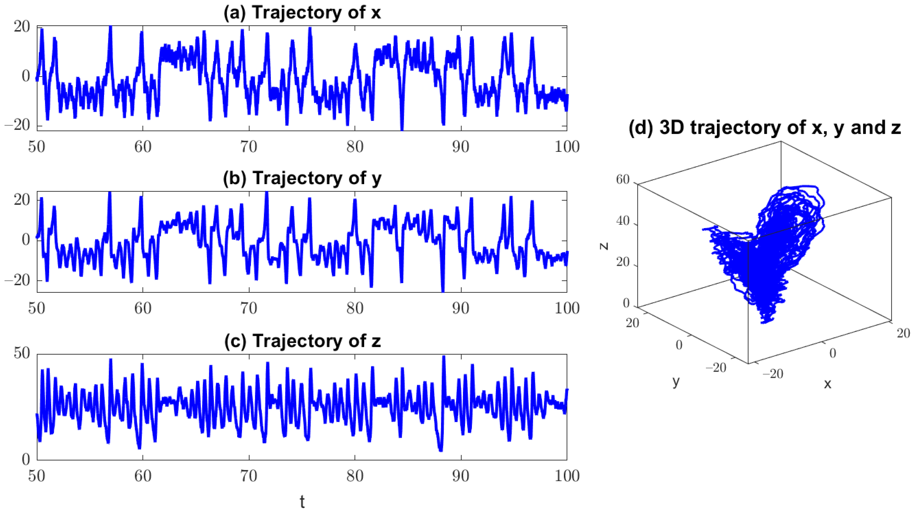
Figure 1 shows one realization of the model simulation. It is clear that the one-dimensional trajectories of the noisy Lorenz 63 model are similar to those from the original deterministic version but with more fluctuations. The chaotic features are illustrated in these time series. The three-dimensional phase plot also clearly indicates a butterfly shape of the model solution.

Assume one realization of the time series y and z is available as the observations. In such a situation, the noisy Lorenz 63 model is a conditional Gaussian system. The new parameter estimation algorithm including the efficient path-wise sampling of the unobserved variable x is thus applicable. To test the parameter estimation skill, the length of the observed time series for y and z is assumed to have 500 time units.

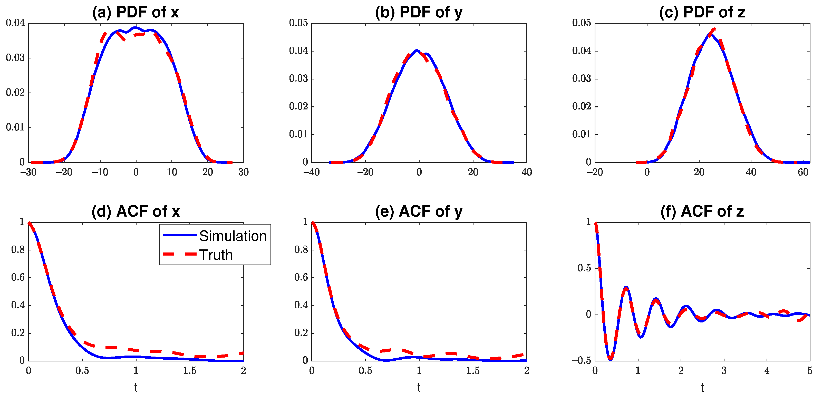
Figure 2 shows the trace plots of the estimated parameters. The initial values of the trace plots start from random numbers that are very different from the truth. After about 200 iterations, all the parameters (except ${\sigma }_x$) converge to the truth, indicating a skillful estimation of these parameters. As a further sanity check, the trace plots of the log-likelihood are also included, which confirm the skill of the algorithm. To understand the behavior of the estimated value of ${\sigma }_x$, it is important to note that ${\sigma }_x$ is the noise coefficient in the unobserved variable. In fact, it has only weak contributions to the fluctuation of the observed time series y and z in the presence of the additional random noise from ${\sigma }_y$ and ${\sigma }_z$. In other words, the parameter ${\sigma }_x$ is only weakly identified in such a chaotic system. Therefore, it is anticipated that the estimation of ${\sigma }_x$ is not as accurate as other parameters. Nevertheless, as is shown in Figure 3, the model with the estimated parameters succeeds in capturing the key statistics of the true signal. In particular, the non-Gaussian PDF of x and the oscillating temporal autocorrelation function (ACF), which measures the memory, of z are both recovered with high accuracy. These results confirm the skill of the estimated parameters.

4.2. A Stochastically Coupled FitzHugh–Nagumo (FHN) Model

The FitzHugh–Nagumo model (FHN) is a prototype system that describes the excitable medium. It aims at characterizing the activation and deactivation dynamics of a spiking neuron [73]. Stochastic versions of the FHN model mimic more realistic situations, where noise-induced limit cycles were widely studied and applied in the context of stochastic resonance [74,75,76,77]. With these desirable dynamical and statistical features, FHN models have applications in many other areas [78,79,80,81].

The stochastically coupled FHN model considered here is as follows:

$$\begin{array}{cc}\hfill \mathrm{d}u& =e\left(u-\frac{1}{3}{u}^3-v\right)\mathrm{d}t+{\sigma }_u\mathrm{d}{W}_u,\hfill \\ \hfill \mathrm{d}v& =(u+a)\mathrm{d}t+{\sigma }_v\mathrm{d}{W}_v.\hfill \end{array}$$

(14)

In (14), the parameter e is a crucial one that represents the time scale ratio. The time scale here is characterized by $ϵ:=1/e$, which is much smaller than one (e.g., $ϵ={10}^{-2}$), implying that u is a fast variable while v is a slow variable. The parameter a is another key parameter that controls the dynamical behavior of the FHN model. The value $a>1$ is required in order to guarantee that the system has a global attractor in the absence of noise and diffusion. However, the random noise is able to drive the system above the threshold level of global stability and triggers limit cycles intermittently that enriches the dynamical features.

The stochastically coupled FHN model (14) is used as the test model for the parameter estimation algorithm. The model (14) has a single neuron, and it contains the model families with both coherence resonance and self-induced stochastic resonance. The model fits into the conditional Gaussian nonlinear modeling framework, where the observed variable is u and the hidden variable is v. With different choices of the noise strength ${\sigma }_v$, (14) exhibits rich dynamical behaviors. The following two regimes are considered for the parameter estimation experiments.

Regime 1: Coherent temporal pattern and nearly regular oscillations. In this dynamical regime, the temporal patterns are highly coherent due to the choice of a weak noise ${\sigma }_v$. The time series of both u and v have nearly regular oscillations with large bursts in u around every fixed number of units. The associated statistical equilibrium PDF of u is bimodal while that of v is skewed. The following parameters are adopted to generate the true time series for regime 1:

$$e=100,a=1.1,{\sigma }_u=2,{\sigma }_v=0.3.$$

(15)

Regime 2: Mixed temporal pattern and irregular oscillations. In this dynamical regime, the temporal patterns are strongly mixed due to the choice of strong noise ${\sigma }_v$. The oscillation period of u becomes more irregular as in regime 1. Correspondingly, the PDF of v becomes nearly Gaussian with a large variance. In addition, a small a is adopted in this regime, leading to a relatively short time between two consecutive excitations of u. The following parameters are adopted to generate the true time series for regime 2:

$$e=100,a=0.8,{\sigma }_u=2,{\sigma }_v=1.5.$$

(16)

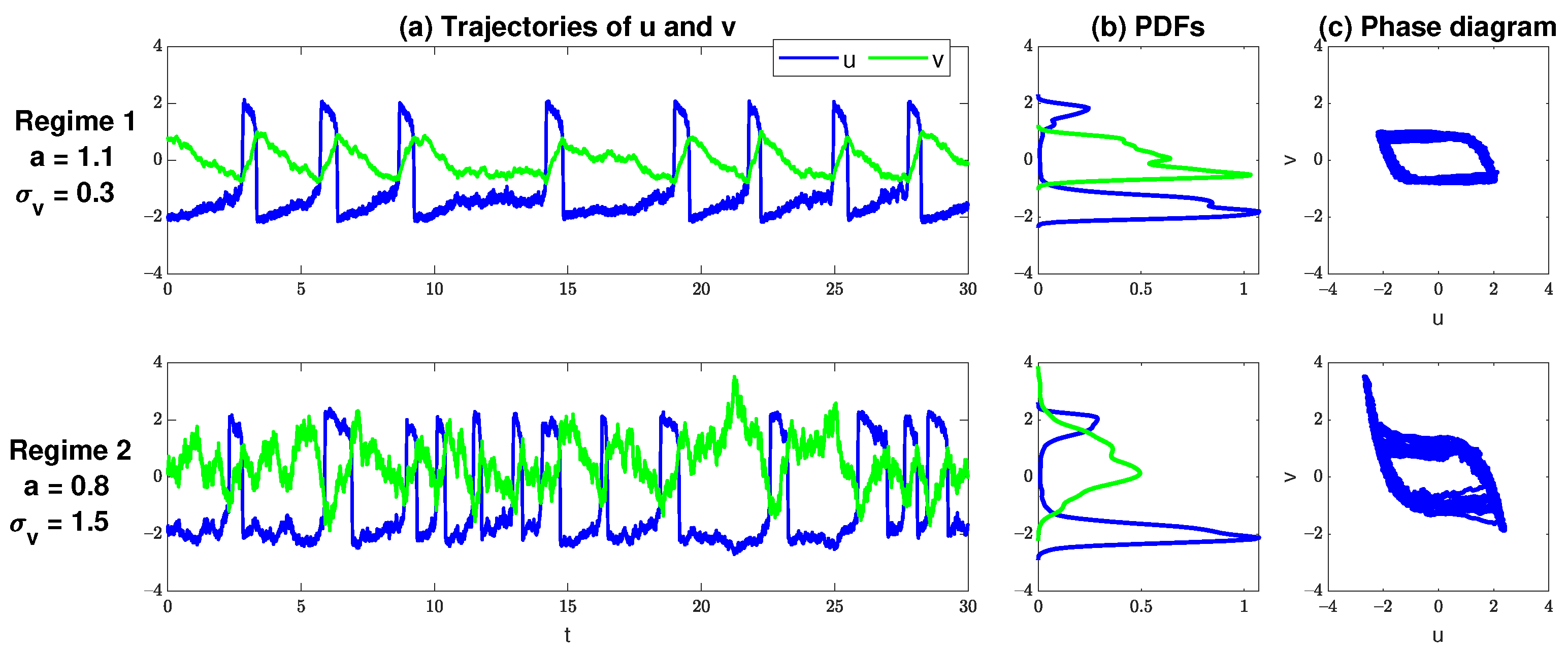
Figure 4 includes the time series, the PDFs, and the phase diagrams of the two dynamical regimes. It is clear that both dynamical regimes have strong non-Gaussian features, where a bimodal distribution is seen in u. Such a bimodal distribution corresponds to a highly intermittent time series with strong extreme events. Regime 1 also has a highly skewed PDF of v, as was described above.

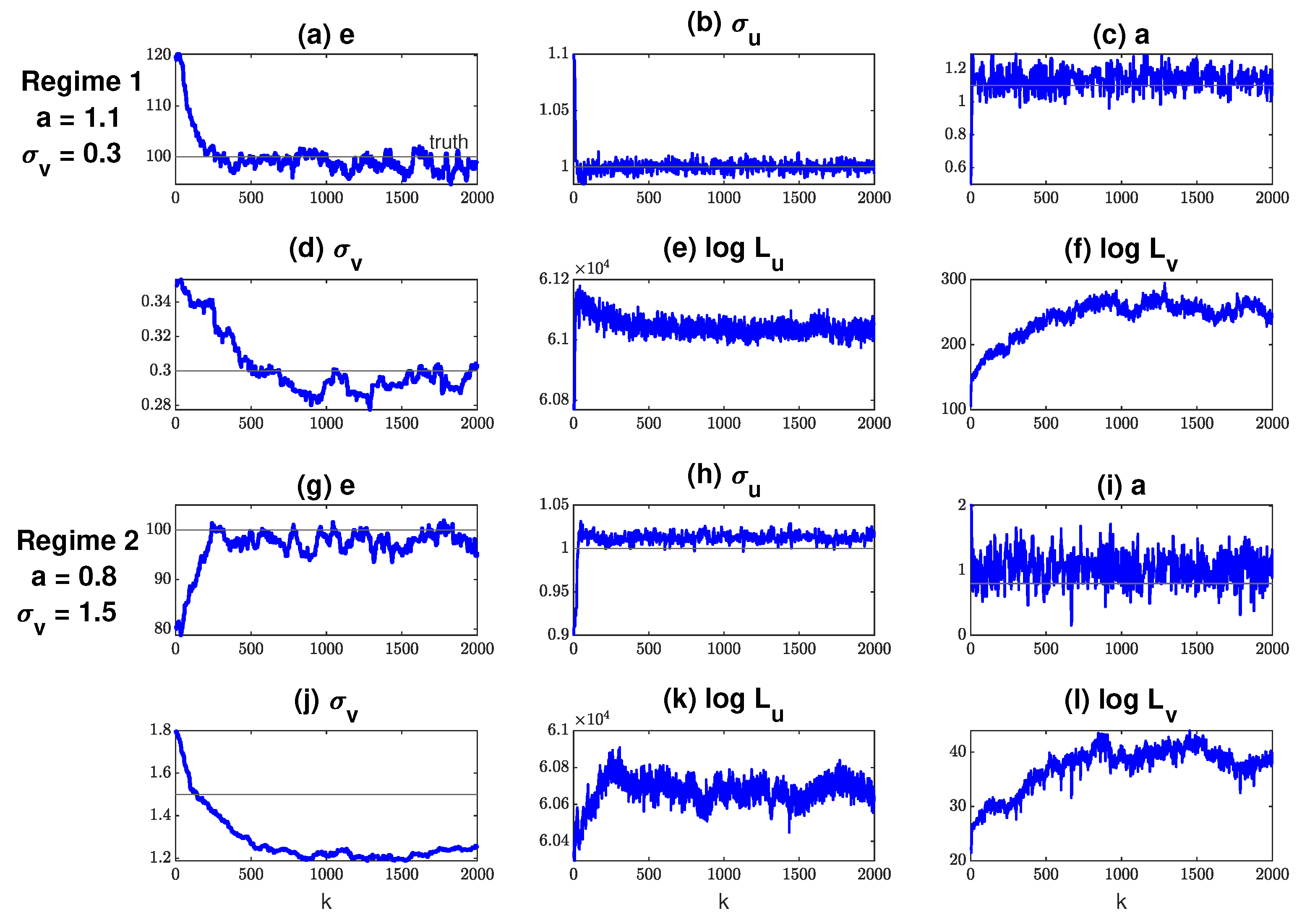
In the setup of parameter estimation, only a single realization of u is available. The total length of the observed u is only 30 time units, representing a moderately short observational period. Figure 5 shows the trace plots of the parameter estimation. Despite being started from a random initial condition, most of the parameters converge quickly to the truth. The only exception is ${\sigma }_v$ in regime 2. This is again understandable because regime 2 is more turbulent and the parameter ${\sigma }_v$ is hard to be identified from the noisy observations. Nevertheless, such a weak identification property also means the feedback from ${\sigma }_v$ to the observed process u is not strong, and therefore the estimated parameters can still recover the significant nonlinear and non-Gaussian features of the true dynamics, especially for the observed variable u.

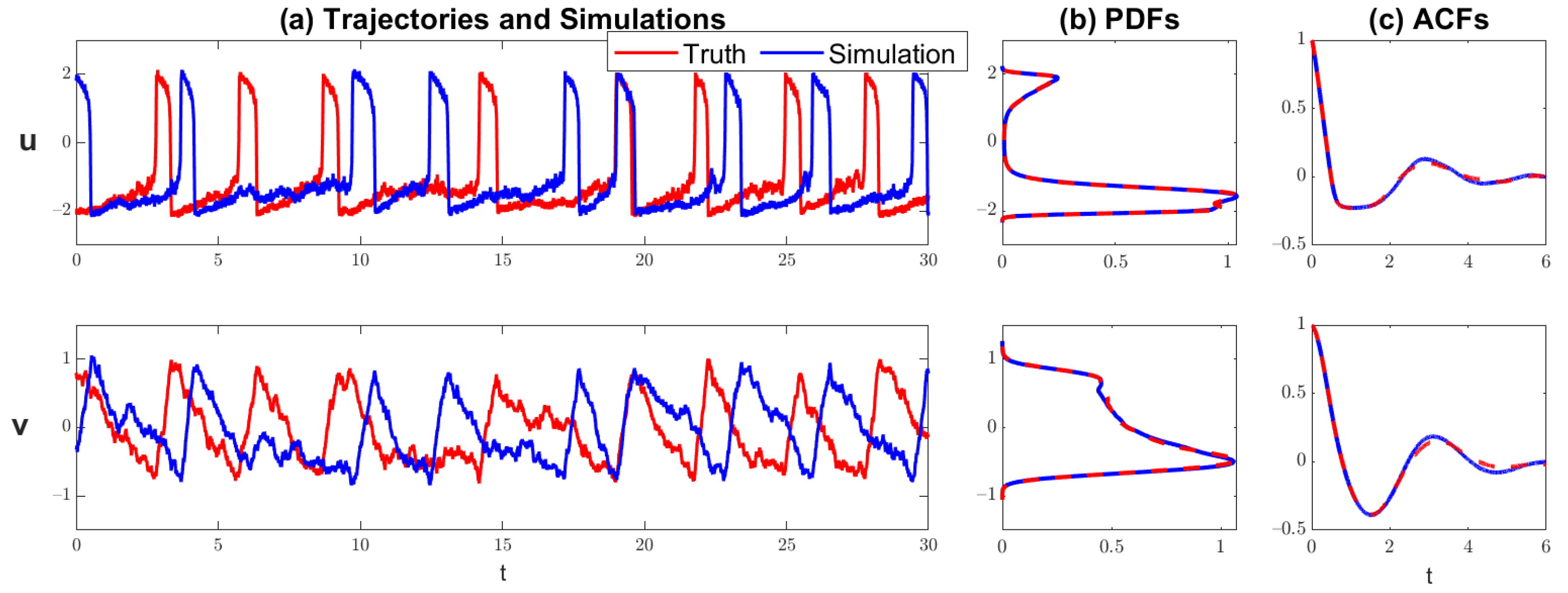
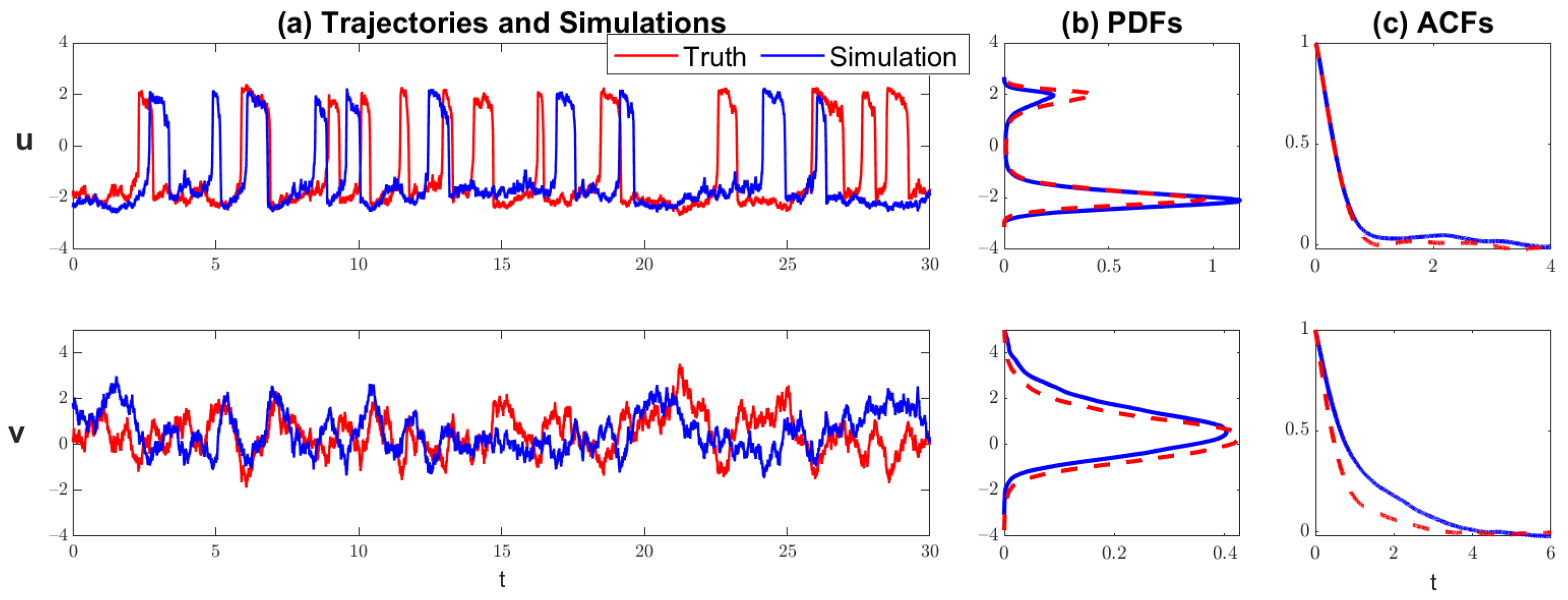
Figure 6 and Figure 7 show the comparison of the model with the true parameters and that with the estimated parameters. Note that the trajectories are computed with different random noise seeds in the two runs. Therefore, the trajectories are not expected to be point-wise consistent with each other. Nevertheless, the overall behavior of the trajectories from the model with the estimated parameters resembles that of the truth. In particular, the model with the estimated parameters generates similar intermittent time series with strong extreme events as the truth. In addition, the statistics from the model with the estimated parameters are also very close to the truth. In regime 1, the highly non-Gaussian PDFs and the irregularly oscillating-decaying ACFs are both perfectly captured by the model with the estimated parameters. In the even tougher dynamical regime 2, despite the small error, the ACFs and the PDFs are still recovered with high accuracy.

5. Conclusions

In this paper, a parameter estimation algorithm is developed for a rich class of complex nonlinear and non-Gaussian turbulent dynamical models using only partial observations. The algorithm follows a data augmentation technique, which allows updating the estimated parameters and the trajectories of the unobserved variables alternatively within a Bayesian MCMC framework. Different from the traditional path-wise sampling methods, the method proposed here exploits the mathematical structure of the class of nonlinear systems, which facilitates the development of a closed analytic formula to sample the trajectories of the unobserved variables. Therefore, the sampling approach is mathematically exact and computationally efficient. The parameter estimation algorithm is applied to both the noisy Lorenz 63 model, which is a highly chaotic system, and a stochastically coupled FHN model, which is a highly nonlinear model with strong non-Gaussian statistics and extreme events.

The test models used in this study are still simple low-dimensional models. Nevertheless, the closed analytic formula of the sampling technique should allow an efficient path-wise sampling for even high-dimensional systems. This will be left as a future work. The rigorous mathematical study of the convergence of the algorithm is another future work.

References

- Majda, A.J. Introduction to Turbulent Dynamical Systems in Complex Systems; Springer: Berlin/Heidelberg, Germany, 2016. [Google Scholar]
- Strogatz, S.H. Nonlinear Dynamics and Chaos with Student Solutions Manual: With Applications to Physics, Biology, Chemistry, and Engineering; CRC Press: Boca Raton, FL, USA, 2018. [Google Scholar]
- Wilcox, D.C. Multiscale model for turbulent flows. AIAA J. 1988, 26, 1311–1320. [Google Scholar] [CrossRef]
- Sheard, S.A.; Mostashari, A. Principles of complex systems for systems engineering. Syst. Eng. 2009, 12, 295–311. [Google Scholar] [CrossRef]
- Law, K.; Stuart, A.; Zygalakis, K. Data Assimilation; Springer: Cham, Switzerland, 2015; Volume 214. [Google Scholar]
- Majda, A.J.; Harlim, J. Filtering Complex Turbulent Systems; Cambridge University Press: Cambridge, UK, 2012. [Google Scholar]
- Farazmand, M.; Sapsis, T.P. Extreme events: Mechanisms and prediction. Appl. Mech. Rev. 2019, 71, 050801. [Google Scholar] [CrossRef] [Green Version]
- Moffatt, H. Extreme events in turbulent flow. J. Fluid Mech. 2021, 914. [Google Scholar] [CrossRef]
- Majda, A.J.; Branicki, M. Lessons in uncertainty quantification for turbulent dynamical systems. Discret. Contin. Dyn. Syst. A 2012, 32, 3133–3221. [Google Scholar] [CrossRef] [Green Version]
- Vlachas, P.R.; Byeon, W.; Wan, Z.Y.; Sapsis, T.P.; Koumoutsakos, P. Data-driven forecasting of high-dimensional chaotic systems with long short-term memory networks. Proc. R. Soc. A Math. Phys. Eng. Sci. 2018, 474, 20170844. [Google Scholar] [CrossRef] [Green Version]
- Feigenbaum, M.J. The transition to aperiodic behavior in turbulent systems. Commun. Math. Phys. 1980, 77, 65–86. [Google Scholar] [CrossRef]
- Bertozzi, A.L.; Luo, X.; Stuart, A.M.; Zygalakis, K.C. Uncertainty quantification in the classification of high dimensional data. arXiv 2017, arXiv:1703.08816. [Google Scholar]
- Köppen, M. The curse of dimensionality. In Proceedings of the 5th Online World Conference on Soft Computing in Industrial Applications (WSC5), Online, 4–8 September 2000; Volume 1, pp. 4–8. [Google Scholar]
- Chen, N.; Majda, A.J. Efficient statistically accurate algorithms for the Fokker—Planck equation in large dimensions. J. Comput. Phys. 2018, 354, 242–268. [Google Scholar] [CrossRef] [Green Version]
- Gershgorin, B.; Majda, A.J. Filtering a statistically exactly solvable test model for turbulent tracers from partial observations. J. Comput. Phys. 2011, 230, 1602–1638. [Google Scholar] [CrossRef]
- Kalnay, E. Atmospheric Modeling, Data Assimilation and Predictability; Cambridge University Press: Cambridge, UK, 2003. [Google Scholar]
- Lau, W.K.M.; Waliser, D.E. Intraseasonal Variability in the Atmosphere-Ocean Climate System; Springer Science & Business Media: Berlin/Heidelberg, Germany, 2011. [Google Scholar]
- Vallis, G.K. Atmospheric and Oceanic Fluid Dynamics; Cambridge University Press: Cambridge, UK, 2017. [Google Scholar]
- Salmon, R. Lectures on Geophysical Fluid Dynamics; Oxford University Press: Oxford, UK, 1998. [Google Scholar]
- Majda, A.J.; Chen, N. Model error, information barriers, state estimation and prediction in complex multiscale systems. Entropy 2018, 20, 644. [Google Scholar] [CrossRef] [Green Version]
- Schittkowski, K. Numerical Data Fitting in Dynamical Systems: A Practical Introduction with Applications and Software; Springer Science & Business Media: Berlin/Heidelberg, Germany, 2002; Volume 77. [Google Scholar]
- Särkkä, S. Bayesian Filtering and Smoothing; Cambridge University Press: Cambridge, UK, 2013; Volume 3. [Google Scholar]
- Rodriguez-Fernandez, M.; Mendes, P.; Banga, J.R. A hybrid approach for efficient and robust parameter estimation in biochemical pathways. Biosystems 2006, 83, 248–265. [Google Scholar] [CrossRef]
- Kokkala, J.; Solin, A.; Särkkä, S. Expectation maximization based parameter estimation by sigma-point and particle smoothing. In Proceedings of the 17th International Conference on Information Fusion (FUSION), Salamanca, Spain, 7–10 July 2014; pp. 1–8. [Google Scholar]
- Chen, N. Learning nonlinear turbulent dynamics from partial observations via analytically solvable conditional statistics. J. Comput. Phys. 2020, 418, 109635. [Google Scholar] [CrossRef]
- Jia, H.; Zhang, Z.; Liu, H.; Dai, F.; Liu, Y.; Leng, J. An approach based on expectation-maximization algorithm for parameter estimation of Lamb wave signals. Mech. Syst. Signal Process. 2019, 120, 341–355. [Google Scholar] [CrossRef]
- Yokoyama, N. Parameter estimation of aircraft dynamics via unscented smoother with expectation-maximization algorithm. J. Guid. Control. Dyn. 2011, 34, 426–436. [Google Scholar] [CrossRef]
- Beck, J.V.; Arnold, K.J. Parameter Estimation in Engineering and Science; Wiley: Hoboken, NJ, USA, 1977. [Google Scholar]
- Aster, R.C.; Borchers, B.; Thurber, C.H. Parameter Estimation and Inverse Problems; Elsevier: Amsterdam, The Netherlands, 2018. [Google Scholar]
- Tarantola, A. Inverse Problem Theory and Methods for Model Parameter Estimation; SIAM: Philadelphia, PA, USA, 2005. [Google Scholar]
- Biegler, L.; Damiano, J.; Blau, G. Nonlinear parameter estimation: A case study comparison. AIChE J. 1986, 32, 29–45. [Google Scholar] [CrossRef]
- Van den Bos, A. Parameter Estimation for Scientists and Engineers; John Wiley & Sons: Hoboken, NJ, USA, 2007. [Google Scholar]
- Branicki, M.; Chen, N.; Majda, A.J. Non-Gaussian test models for prediction and state estimation with model errors. Chin. Ann. Math. Ser. B 2013, 34, 29–64. [Google Scholar] [CrossRef] [Green Version]
- Richey, M. The evolution of Markov chain Monte Carlo methods. Am. Math. Mon. 2010, 117, 383–413. [Google Scholar] [CrossRef] [Green Version]
- Haario, H.; Laine, M.; Mira, A.; Saksman, E. DRAM: Efficient adaptive MCMC. Stat. Comput. 2006, 16, 339–354. [Google Scholar] [CrossRef]
- Raftery, A.E.; Lewis, S.M. Implementing mcmc. Markov chain Monte Carlo in Practice; CRC Press: Boca Raton, FL, USA, 1995; pp. 115–130. [Google Scholar]
- Tanner, M.A.; Wong, W.H. The calculation of posterior distributions by data augmentation. J. Am. Stat. Assoc. 1987, 82, 528–540. [Google Scholar] [CrossRef]
- Roberts, G.O.; Stramer, O. On inference for partially observed nonlinear diffusion models using the Metropolis–Hastings algorithm. Biometrika 2001, 88, 603–621. [Google Scholar] [CrossRef] [Green Version]
- Beskos, A.; Roberts, G.O. Exact simulation of diffusions. Ann. Appl. Probab. 2005, 15, 2422–2444. [Google Scholar] [CrossRef] [Green Version]
- Cotter, S.L.; Roberts, G.O.; Stuart, A.M.; White, D. MCMC methods for functions: Modifying old algorithms to make them faster. Stat. Sci. 2013, 28, 424–446. [Google Scholar] [CrossRef]
- Chib, S.; Pitt, M.K.; Shephard, N. Likelihood Based Inference for Diffusion Driven Models. 2004. Available online: http://www.nuff.ox.ac.uk/economics/papers/2004/w20/chibpittshephard.pdf (accessed on 1 August 2004).
- Kalogeropoulos, K. Likelihood-based inference for a class of multivariate diffusions with unobserved paths. J. Stat. Plan. Inference 2007, 137, 3092–3102. [Google Scholar] [CrossRef] [Green Version]
- Papaspiliopoulos, O.; Roberts, G.O.; Stramer, O. Data augmentation for diffusions. J. Comput. Graph. Stat. 2013, 22, 665–688. [Google Scholar] [CrossRef] [Green Version]
- Stramer, O.; Bognar, M. Bayesian inference for irreducible diffusion processes using the pseudo-marginal approach. Bayesian Anal. 2011, 6, 231–258. [Google Scholar] [CrossRef]
- Chen, N.; Giannakis, D.; Herbei, R.; Majda, A.J. An MCMC algorithm for parameter estimation in signals with hidden intermittent instability. SIAM/ASA J. Uncertain. Quantif. 2014, 2, 647–669. [Google Scholar] [CrossRef] [Green Version]
- Golightly, A.; Wilkinson, D.J. Bayesian inference for stochastic kinetic models using a diffusion approximation. Biometrics 2005, 61, 781–788. [Google Scholar] [CrossRef]
- Golightly, A.; Wilkinson, D.J. Bayesian sequential inference for nonlinear multivariate diffusions. Stat. Comput. 2006, 16, 323–338. [Google Scholar] [CrossRef]
- Golightly, A.; Wilkinson, D.J. Bayesian sequential inference for stochastic kinetic biochemical network models. J. Comput. Biol. 2006, 13, 838–851. [Google Scholar] [CrossRef]
- Chen, N.; Majda, A. Conditional Gaussian systems for multiscale nonlinear stochastic systems: Prediction, state estimation and uncertainty quantification. Entropy 2018, 20, 509. [Google Scholar] [CrossRef] [PubMed] [Green Version]
- Chen, N.; Majda, A.J. Filtering nonlinear turbulent dynamical systems through conditional Gaussian statistics. Mon. Weather Rev. 2016, 144, 4885–4917. [Google Scholar] [CrossRef]
- Liptser, R.S.; Shiryaev, A.N. Statistics of Random Processes II: Applications; Springer Science & Business Media: Berlin/Heidelberg, Germany, 2013; Volume 6. [Google Scholar]
- Chen, N.; Majda, A.J.; Tong, X.T. Information barriers for noisy Lagrangian tracers in filtering random incompressible flows. Nonlinearity 2014, 27, 2133. [Google Scholar] [CrossRef] [Green Version]
- Chen, N.; Majda, A.J.; Tong, X.T. Noisy Lagrangian tracers for filtering random rotating compressible flows. J. Nonlinear Sci. 2015, 25, 451–488. [Google Scholar] [CrossRef]
- Chen, N.; Majda, A.J. Model error in filtering random compressible flows utilizing noisy Lagrangian tracers. Mon. Weather Rev. 2016, 144, 4037–4061. [Google Scholar] [CrossRef]
- Chen, N.; Majda, A.J.; Giannakis, D. Predicting the cloud patterns of the Madden-Julian Oscillation through a low-order nonlinear stochastic model. Geophys. Res. Lett. 2014, 41, 5612–5619. [Google Scholar] [CrossRef]
- Chen, N.; Majda, A.J. Predicting the real-time multivariate Madden–Julian oscillation index through a low-order nonlinear stochastic model. Mon. Weather Rev. 2015, 143, 2148–2169. [Google Scholar] [CrossRef]
- Chen, N.; Majda, A.J.; Sabeerali, C.; Ajayamohan, R. Predicting monsoon intraseasonal precipitation using a low-order nonlinear stochastic model. J. Clim. 2018, 31, 4403–4427. [Google Scholar] [CrossRef] [Green Version]
- Chen, N.; Majda, A.J. Beating the curse of dimension with accurate statistics for the Fokker—Planck equation in complex turbulent systems. Proc. Natl. Acad. Sci. USA 2017, 114, 12864–12869. [Google Scholar] [CrossRef] [Green Version]
- Chen, N.; Majda, A.J.; Tong, X.T. Spatial localization for nonlinear dynamical stochastic models for excitable media. arXiv 2019, arXiv:1901.07318. [Google Scholar] [CrossRef] [Green Version]
- Oksendal, B. Stochastic Differential Equations: An Introduction with Applications; Springer Science & Business Media: Berlin/Heidelberg, Germany, 2013. [Google Scholar]
- Chen, N.; Majda, A.J. Efficient Nonlinear Optimal Smoothing and Sampling Algorithms for Complex Turbulent Nonlinear Dynamical Systems with Partial Observations. J. Comput. Phys. 2020, 410, 109381. [Google Scholar] [CrossRef]
- Vihola, M. Robust adaptive Metropolis algorithm with coerced acceptance rate. Stat. Comput. 2012, 22, 997–1008. [Google Scholar] [CrossRef] [Green Version]
- Gardiner, C.W. Handbook of Stochastic Methods for Physics, Chemistry and the Natural Sciences; Springer: Berlin/Heidelberg, Germany, 2004; Volume 13. [Google Scholar]
- Lorenz, E.N. Deterministic nonperiodic flow. J. Atmos. Sci. 1963, 20, 130–141. [Google Scholar] [CrossRef] [Green Version]
- Sparrow, C. The Lorenz Equations: Bifurcations, Chaos, and Strange Attractors; Springer Science & Business Media: Berlin/Heidelberg, Germany, 2012; Volume 41. [Google Scholar]
- Haken, H. Analogy between higher instabilities in fluids and lasers. Phys. Lett. A 1975, 53, 77–78. [Google Scholar] [CrossRef]
- Knobloch, E. Chaos in the segmented disc dynamo. Phys. Lett. A 1981, 82, 439–440. [Google Scholar] [CrossRef]
- Gorman, M.; Widmann, P.; Robbins, K. Nonlinear dynamics of a convection loop: A quantitative comparison of experiment with theory. Phys. D Nonlinear Phenom. 1986, 19, 255–267. [Google Scholar] [CrossRef]
- Hemati, N. Strange attractors in brushless DC motors. IEEE Trans. Circuits Syst. I Fundam. Theory Appl. 1994, 41, 40–45. [Google Scholar] [CrossRef]
- Cuomo, K.M.; Oppenheim, A.V. Circuit implementation of synchronized chaos with applications to communications. Phys. Rev. Lett. 1993, 71, 65. [Google Scholar] [CrossRef] [PubMed]
- Poland, D. Cooperative catalysis and chemical chaos: A chemical model for the Lorenz equations. Phys. D Nonlinear Phenom. 1993, 65, 86–99. [Google Scholar] [CrossRef]
- Tzenov, S.I. Strange attractors characterizing the osmotic instability. arXiv 2014, arXiv:1406.0979. [Google Scholar]
- Lindner, B.; Garcıa-Ojalvo, J.; Neiman, A.; Schimansky-Geier, L. Effects of noise in excitable systems. Phys. Rep. 2004, 392, 321–424. [Google Scholar] [CrossRef]
- Treutlein, H.; Schulten, K. Noise Induced Limit Cycles of the Bonhoeffer-Van der Pol Model of Neural Pulses. Ber. Bunsenges Phys. Chem. 1985, 89, 710–718. [Google Scholar] [CrossRef]
- Lindner, B.; Schimansky-Geier, L. Coherence and stochastic resonance in a two-state system. Phys. Rev. E 2000, 61, 6103. [Google Scholar] [CrossRef] [PubMed] [Green Version]
- Longtin, A. Stochastic resonance in neuron models. J. Stat. Phys. 1993, 70, 309–327. [Google Scholar] [CrossRef] [Green Version]
- Wiesenfeld, K.; Pierson, D.; Pantazelou, E.; Dames, C.; Moss, F. Stochastic resonance on a circle. Phys. Rev. Lett. 1994, 72, 2125. [Google Scholar] [CrossRef]
- Neiman, A.; Schimansky-Geier, L.; Cornell-Bell, A.; Moss, F. Noise-enhanced phase synchronization in excitable media. Phys. Rev. Lett. 1999, 83, 4896. [Google Scholar] [CrossRef]
- Hempel, H.; Schimansky-Geier, L.; Garcia-Ojalvo, J. Noise-sustained pulsating patterns and global oscillations in subexcitable media. Phys. Rev. Lett. 1999, 82, 3713. [Google Scholar] [CrossRef]
- Hu, B.; Zhou, C. Phase synchronization in coupled nonidentical excitable systems and array-enhanced coherence resonance. Phys. Rev. E 2000, 61, R1001. [Google Scholar] [CrossRef] [Green Version]
- Jung, P.; Cornell-Bell, A.; Madden, K.S.; Moss, F. Noise-induced spiral waves in astrocyte syncytia show evidence of self-organized criticality. J. Neurophysiol. 1998, 79, 1098–1101. [Google Scholar] [CrossRef]
Figure 1.
The noisy Lorenz 63 model (12) with parameters in (13). (a–c) one realization of the one-dimensional trajectories of , respectively; (d) the associated three-dimensional phase plot of .
Figure 2.
Trace plots of the estimated parameters in the noisy Lorenz 63 model. (a–f) the trace plots of each individual parameters , and . For reference, the true parameters are shown by the black solid lines; (g) the trace plot of the log-likelihood for the hidden path of x, according to (6); (h–i) the trace plots of the log-likelihood of the observation of y and z, respectively, according to (5); (j) the trace plots of the total log-likelihood.
Figure 3.
Comparison of the PDFs and ACFs of a long simulation from the noisy Lorenz 63 model with the true parameters (13) (dashed red curves) and that with the estimated parameters (solid blue curve). The last point in each of the trace plots is regarded as the estimated value of each parameter.
Figure 4.
The two dynamical regimes of the stochastically coupled FHN model (14), where the parameters of the two regimes are listed in (15) and (16). The three columns show the model trajectories, the PDFs, and the phase diagram of both dynamical regimes.
Figure 5.
Trace plot of the estimated parameters in the stochastically coupled FHN model (14) for dynamical regime 1 (top 2 rows) and 2 (bottom 2 rows). (a–d,g–j) the trace plots of the parameters , and . For reference, the true parameter values are shown by the black lines; (e,k) the trace plot of the log-likelihood of the observation of u, according to (5); (f,l) the trace plot of the log-likelihood for the hidden path of v, according to (6).
Figure 6.
Comparison of the models with the true parameters (dashed red curves) and with the estimated parameters (solid blue curve) for dynamical regime 1. The last point in each of the trace plots is regarded as the estimated value of each parameter. (a) the comparison of the trajectories. Note that the trajectories are computed with different random noise seeds in the two runs. Therefore, the trajectories are not expected to be point-wise consistent with each other; (b,c) the comparisons of the PDFs and the ACFs.
Figure 7.
Similar to Figure 6 but for dynamical regime 2.
Publisher’s Note: MDPI stays neutral with regard to jurisdictional claims in published maps and institutional affiliations. |
© 2021 by the authors. Licensee MDPI, Basel, Switzerland. This article is an open access article distributed under the terms and conditions of the Creative Commons Attribution (CC BY) license (https://creativecommons.org/licenses/by/4.0/).
Share and Cite
MDPI and ACS Style
Zhang, Z.; Chen, N. Parameter Estimation of Partially Observed Turbulent Systems Using Conditional Gaussian Path-Wise Sampler. Computation 2021, 9, 91. https://0-doi-org.brum.beds.ac.uk/10.3390/computation9080091
AMA Style
Zhang Z, Chen N. Parameter Estimation of Partially Observed Turbulent Systems Using Conditional Gaussian Path-Wise Sampler. Computation. 2021; 9(8):91. https://0-doi-org.brum.beds.ac.uk/10.3390/computation9080091
Chicago/Turabian StyleZhang, Ziheng, and Nan Chen. 2021. "Parameter Estimation of Partially Observed Turbulent Systems Using Conditional Gaussian Path-Wise Sampler" Computation 9, no. 8: 91. https://0-doi-org.brum.beds.ac.uk/10.3390/computation9080091
Note that from the first issue of 2016, this journal uses article numbers instead of page numbers. See further details here.