Use of Response Time for Measuring Cognitive Ability

Abstract

The purpose of this paper is to review some of the key literature on response time as it has played a role in cognitive ability measurement, providing a historical perspective as well as covering current research. We discuss the speed-level distinction, dimensions of speed and level in cognitive abilities frameworks, speed–accuracy tradeoff, approaches to addressing speed–accuracy tradeoff, analysis methods, particularly item response theory-based, response time models from cognitive psychology (ex-Gaussian function, and the diffusion model), and other uses of response time in testing besides ability measurement. We discuss several new methods that can be used to provide greater insight into the speed and level aspects of cognitive ability and speed–accuracy tradeoff decisions. These include item-level time limits, the use of feedback (e.g., CUSUMs), explicit scoring rules that combine speed and accuracy information (e.g., count down timing), and cognitive psychology models. We also review some of the key psychometric advances in modeling speed and level, which combine speed and ability measurement, address speed–accuracy tradeoff, allow for distinctions between response times on items responded to correctly and incorrectly, and integrate psychometrics with information-processing modeling. We suggest that the application of these models and tools is likely to advance both the science and measurement of human abilities for theory and applications.

1. Introduction

Response time has always been a concern in ability measurement, sometimes implicitly as in time-limit tests, sometimes explicitly as in so-called speeded tests, and sometimes as the main outcome variable as in reaction time, or information-processing tests. The measurement of processing speed per se also has been a part of testing since its earliest days. For example, ability measurement pioneers Galton [1] and Spearman [2] administered reaction time measures. However, the use of computerized testing has led to significant development of models of response time because item response time is often automatically collected.

A major challenge in the measurement of response time is that there are many factors that influence it, and it is typically impossible to attribute response time uniquely to any particular factor. For example, a respondent’s slow response might reflect either slow processing speed or carefulness. A respondent may respond quickly and correctly because of a lucky guess, or slowly and correctly, but could have answered correctly quickly if incentivized to do so. If a respondent does not answer correctly, it could be due to not knowing the answer, not spending enough time to process the information fully, or having gotten confused while answering and quitting. Although there is generally a tradeoff between speed and accuracy in responding, the tradeoff is not fixed, across tasks, or people; and a respondent may answer more accurately under time pressure than with unlimited time; or as Duke Ellington put it, “I don’t need time, I need a deadline.”

The purpose of this paper is to review some of the key literature on response time as it has played a role in cognitive ability measurement. We discuss the speed-level distinction, dimensions of speed and level in cognitive abilities frameworks, speed–accuracy tradeoff, approaches to addressing speed–accuracy tradeoff, analysis methods, particularly item response theory-based, and other uses of response time in testing besides ability measurement. We also discuss two cognitive information-processing treatments of response time, the ex-Gaussian function and the diffusion model. This paper is not intended to be a comprehensive review (see reviews [3,4,5,6]). Rather it is intended to highlight significant recent developments in the use of response time for measuring cognitive ability set in the context of a historical perspective.

2. Speed-Level Distinction

The distinction between how quickly one can solve problems (speed) and how difficult a problem one can solve (level) has been made in ability testing for a long time [7].1 These two performance dimensions, speed and level, have typically been measured with simple speeded tests where the primary outcome measure is the number correct in a given time (or the time taken to complete a fixed number of items), and complex power tests, designed to measure one’s ability level, where the primary outcome is the number correct under liberal or no time limits. Others [8,9] preferred degree of speeding to the speed–power dichotomy, and defined a test as completely unspeeded “when no subject’s standing would be altered if he were given additional time” and a test as speeded to the extent that “the time limit alters, not his score, but his true standard score in the group” (p. 184 in [8]). However, these are theoretical definitions, and there have been practical attempts to define a speeded vs. a power test. ETS test development policies have addressed definitions of test speededness [10,11]. A form of a major standardized test was considered unspeeded if (a) all test takers finish at least 75% of the items (or respond to at least one question beyond three-fourths of the way through a section); and (b) at least 80% of the students respond to all items (or reach the last question).2

A recurring question has been whether speed and level are simply two interchangeable measures of the same underlying ability or whether they represent different constructs. The first key study on this issue [13] administered a battery of paper-and-pencil tests to students with instructions to switch colored pencils for marking answers after a certain time had passed, then to complete the test without a time limit. For each test, the total number of correct responses (level score), the number of correct responses within the time limit (time-limit score), and the time taken to finish (speed score) were recorded. (Note that although referred to here as a “speed score,” time-taken-to-finish reflects both work rate and the test taker’s choice as to when to stop working.) A factor analysis of the level and speed scores was conducted with the time-limit scores later correlated with the factors (by a projection method [14]), which indicated separate speed and level factors, with time-limited scores correlating with both, as might be expected.

This study [13] and others conducted along those lines were limited in their ability to address item response time due to using the paper-and-pencil method. In the 1970s and 1980s with the new availability of microcomputers, along with the cognitive revolution in psychology [15], there was interest in analyzing item responses and item response times where items differed in features designed to systematically vary their information-processing requirements. Mental rotation studies [16], which found that the time to compare two identical or mirror-image diagrams depicted in various spatial orientations was linearly related to their degree of angular disparity, were a paradigmatic example of this approach. It was also widely assumed at the time, at least within the experimental cognitive psychology (as opposed to psychometric) community, that speed and level measures were more or less interchangeable, but that speed measures were preferred because they were more sensitive to experimental manipulations3 and thus more revealing of the underlying cognitive processes. Lohman [17] adopted an item response approach for his dissertation, as he was directly interested in addressing the issue of speed–level interchangeability. He administered a spatial visualization task requiring figure rotation and combination, with figures varying in complexity (number of points on a polygon). He regressed response times on item complexity enabling him to estimate expected times for complex items. From this, he found support for separate speed and level factors, concluding that speed of solving simple items was uncorrelated with probability of being able to solve complex items of the same type (complexity defined as the number of distinct mental operations to perform, the complexity of the figure, and whether the resultant mentally transformed figure matched or did not match a target figure).

Another study that provided support for the independence of speed and level in the verbal realm was one on verbal associative learning [18]. In this study, participants memorized lists of 10 word pairs (e.g., rain—house), made up of common words, presented for a fixed study time (0.5–8 s, per pair), and then were asked to recognize or recall one of the words from each pair (e.g., rain—?). The finding was that one’s vocabulary level (measured separately) was a strong predictor of performance in the recall and recognition tasks, but that one’s verbal speed (measured with a simple word classification test) only predicted performance in the condition with limited study time (0.5 s), and not for conditions with more study time.

3. Dimensions of Speed and Level in the Structure of Human Cognitive Abilities

Probably the most comprehensive framework to date for characterizing the organization of human abilities is the Cattell-Horn-Carroll (CHC) theory [19,20,21,22,23,24]. Most of the empirical support for the framework is found in Carroll’s [19] meta-analysis of 461 datasets each involving the administration of anywhere between five and 99 cognitive ability tests to children, students, and adults of all grade levels and ages mostly (76%) but not exclusively in the United States, between the years 1925 and 1987.

A summary of those data suggested a three stratum framework with a single general cognitive ability at the third stratum, eight abilities at the second stratum, and sixty-six or so first-stratum abilities [19]. Second stratum abilities included fluid, crystallized, memory, visualization, and others. First stratum abilities within the fluid ability category were inductive reasoning, sequential (deductive) reasoning, quantitative reasoning, and Piagetian reasoning. Other second stratum factors similarly were broken down into narrower primary factors.

The factors identified in the meta-analysis [19] can be classified as either level or speed factors, with roughly half being speed factors. At the second stratum, for example, three of the eight factors are speed factors. These include a processing speed factor (Gt) measured by simple and choice reaction time tasks and other speeded tasks (e.g., synonym comparisons for common words). A separate broad cognitive speediness factor (Gs) is measured by numerical facility (e.g., 1 digit addition) and perceptual speed (e.g., letter-picture matching) tests, and rate of test taking (e.g., the number of items checked within a time limit) factors. (A possible reason for the empirical finding of a Gs-Gt distinction is that the former are primarily tests given on computer, and the latter, paper-and-pencil tests, indicating a method distinction [25]. Other studies since have further clarified the dimensionality of processing speed measures [25,26,27].

The third second-stratum factor is a broad retrieval ability factor (Gr) which is measured primarily by fluency tests. Example fluency tests are ones in which an examinee is given, say, 2 min to “list all the 4-letter words that you can think of that begin with B and end with T” or “write down as many synonyms as possible for the word ‘good’.”

In addition, separate speed and level factors of fluid ability (Gf), crystallized ability (Gc), and visual perception ability (Gv) were identified [19]. An example of the speed–level distinction in visual perception is something like speed of matching two simple geometric figures side by side (SR, Spatial Relations), versus probability of being able to successfully match complex three-dimensional figures, or to infer the pattern of holes on a sheet of paper created by punching through a folded up piece of paper (GV, general visualization). In the fluid realm, a typical level test is number series (2 3 6 7 8 16 17 _, choose the next) or letter sets (feg mln bca, choose the odd one) (I, Induction). Early studies identified a speed of reasoning factor (RE, Reasoning Speed), as simply time taken to finish (see above [13]). Using more sophisticated approaches, speed of reasoning factors have been identified in several more recent studies [28,29,30]. In the crystallized realm, writing ability (often measured as the amount of writing accomplished in a time limit) (WA) and reading speed (measured as time to read a passage aloud, or time to read silently while crossing out nonsensical words, or reading under strict time limits) (RS) are correlated with but separable from the level factor of reading comprehension (RC) [19].

One of the more recent studies addressing the issue of the independence of speed and level in the domain of reasoning was based on a time-limit manipulation [30]. Wilhelm and Schulze [30] created two batteries of verbal, figural, and numerical reasoning tasks (e.g., analogies, series, “odd man out” tasks), and administered them either under timed or untimed conditions, where the untimed-condition time limit was 2.5 times the timed-condition time limit. Time limits resulted in mean number correct differences of approximately 1.5–2 standard deviation difference between conditions. They then correlated performance in the two conditions with measures of processing speed and found that (a) timed and untimed reasoning performance was correlated (r = 0.64/0.93, for observed and disattenuated, respectively); but (b) processing speed measures were more highly correlated with performance in the timed (r = 0.49/0.65) than untimed (r = 0.34/0.45) conditions. A confirmatory factor analysis was consistent with the correlation findings.

Carroll’s [19] summary and reanalysis support the notion of separate speed and level factors, on both logical and empirical grounds. Carroll also concluded that general cognitive ability (or “intelligence”) is chiefly a level ability despite a large body of research relating cognitive ability to basic reaction time. At the same time, he admitted that there were many weaknesses in the research done to date, including task models (and scoring models) failing to take into account both speed and level aspects, motivation, tendency to guess, and omissions or abandonments. He also noted that models (at the time of his writing) also tended to ignore the effects of time limits on tests, and did not take into account that the speed–level correlation might be different for different tasks. Many of these weaknesses have been or are beginning to be addressed in new psychometric models, a topic addressed throughout the remainder of this paper.

4. Speed–Accuracy Tradeoff

A limitation of the studies reviewed above [13,17,30], as well as most of the individual differences literature prior to Carroll’s [19] review could be that time to complete a test (or an item) confounds processing speed with the choice of how much time to persist on the task, or when to abandon a solution attempt [31,32]. Those who take a long time to respond to an item might do so because they are careful or because they are slow. If a wrong response is made it is unclear whether spending more time on the item might have eventually led to a correct response. However, in general, it is clear that in just about any task we undertake, from a choice reaction time task on the order of milliseconds, a complex mathematics task on the order of minutes, to a data analysis project on the order of hours, days, or months we can trade off accuracy for speed. A history [33] traces the idea of a speed–accuracy tradeoff in psychological tasks to 1911 [34].

Although test instructions typically inform examinees to “work as quickly as you can without making many errors,” or “you will have 25 min to complete the test,” there is ambiguity in how best to interpret and implement those instructions. Consequently, there have been various proposals for imposing some kind of control over speed–accuracy tradeoff so as to enable meaningful comparisons across individuals. We review some of these methods here.

4.1. Deadline Method (Time Limits)

The traditional time-limit test imposes a deadline to complete a set of items. As Carroll noted, depending on how loose or severe the deadline, the construct can change from a primarily level to primarily speeded construct. This is not always the case. Bridgeman and colleagues conducted several studies varying time limits on experimental math and verbal sections of the SAT [12] and GRE [35] tests. In the SAT study, this was done by manipulating the number of items administered in a fixed 30 min time slot (rather than manipulating slot time [36]), allowing for a comparison between regular time testing (35 items in 30 min) and time-and-a-half time testing (23 items in 30 min). No differences or very small differences were found due to this manipulation. In the GRE study, the time limit itself was manipulated which resulted in only very small effects, essentially replicating the conclusions of an earlier GRE study [37]. For all these studies, the finding of no benefit for more testing time could be due to the fact that regular time testing was not speeded, and so additional time was not helpful. In fact the purpose of the studies was to establish that that was the case.

Time limits have traditionally been set at the test (or test section) level [12]. With computerized administration, it is possible to set deadlines at the item level. This enables a more fine-grained way to address the issue of the confounding of processing time with persistence. In one of the first studies to do this, Lohman [38] borrowed a method commonly used in cognitive psychology [39,40] in which test takers solved problems under varying deadlines (here, mental rotation problems), allowing the estimation of each individual’s speed–accuracy tradeoff curve [41]. The curve fitted was probability correct as a function of exposure time, using an exponential with an intercept (the amount of time needed for the probability of getting an item correct to rise above zero, or chance, assumed to be common to all test takers), a slope (the rate at which probability correct increased with increases in the deadline), and an asymptote (the point at which an examinee’s accuracy no longer increased, even with more time). Low compared to high ability examinees showed a lower asymptote, particularly with more complex item types (e.g., greater mental rotation required), and male-female differences were found at the asymptotic level, rather than in mean response time [38].

Lohman [42] also described applications of varying deadlines to other tasks (spatial and verbal) to produce a speed–accuracy tradeoff curve. He reviewed different ways to produce deadlines and a speed–accuracy tradeoff curve. These include post hoc analysis (e.g., binning by accuracy then plotting response time by accuracy bin), instructions (general instructions, payoffs, specific deadlines, and time intervals), and response signals (e.g., an auditory tone signaling the requirement to provide an immediate response). Following Reed [43], Lohman [42] suggested that with all methods it is useful to conduct two experiments each time, one with conventional instructions (“respond as fast and accurately as possible”) and the other with the experimentally induced speed–accuracy tradeoff. This would enable both accounting for speed–accuracy tradeoff and avoiding the problem of how to treat response times for items incorrectly answered.

Wright and Dennis [44] examined the use of deadlines, also referred to as a time envelope [45], in which examinees respond within a certain time (specifically, one of four levels: either 2, 3, 4, or 5 s). They implemented this method on a reasoning task with linear syllogisms (“Tom is taller than Fred, Fred is shorter than Mike, who’s shortest”). Items for this task could be generated from a set of item models (e.g., a is more x than b, b is more x than c, who’s most x; a is not as x as b, c is not as x as a, who’s most x), known as slot-filler models, in which the variable slots, a, b, c, are filled with names (e.g., John, Mary, Fred), and the variable slot x with comparative adjectives (e.g., tall, strong, fast). There were a total of eight different slot-filler item models, and the assumption was that the eight item models differed from one another in difficulty (and hence, were referred to as radicals). In contrast, the assumption was that the fillers (e.g., John, Mary, Fred) did not affect difficulty (and hence were referred to as incidentals). Wright and Dennis fit what essentially was a one parameter normal-ogive item response theory model to the data (it fixed a guessing parameter at 0.5, and assumed discrimination to be a constant, 1.0, across all items, leaving difficulty as the only free parameter). However, instead of modeling the 44 item responses they modeled item family (the eight item models), and response time deadlines (the four response deadlines), for a total of 12 parameters (minus one fixed parameter, giving 11) (see [46] for a similar approach), treating model type and time envelope as predictors of item difficulty, and found a good fit to the data.4

As this study was presented at a conference, there was discussion about the methodology in a question-and-answer session at the conference immediately after the presentation of the paper, which is recorded in their chapter. Some of the issues addressed concern the feasibility of the method, given the additional testing time required, and the model assumption that time could be treated as simply a difficulty generating factor measuring the same construct as was initially measured by the test. In particular, the issue of the independence of speed and level was not directly addressed; rather it was assumed that manipulating item types and deadlines were equally reasonable methods of making easier or harder test items without changing the construct, a perhaps questionable assumption. Another issue along these lines was a question of whether performance under severe time deadlines was useful to know about in general, and a question about whether performance under severe time limits might tap into an anxiety factor changing the construct assessed (performance under stress, including time limits, is an important topic in its own right [50]). The Wright-Dennis [44] proposal was never implemented operationally; tests in the British Army Recruit Battery (BARB), which was the source for the material they examined, are administered under a test-level time limit.

Goldhammer [3] also proposed the use of deadlines (or variations on deadlines, such as providing a window of time in which to supply an answer) arguing that “single estimates of effective speed and ability can hardly be used to compare individuals” (p. 158 in [3]). This is an intriguing proposal as operational cognitive testing, such as PISA, PIAAC, ASVAB, SAT, GRE, and TOEFL, are all based on a single estimate, typically scale scores, which are transformations of equated number corrects (equating adjusts for form differences in difficulty), in a time-limit test. Goldhammer’s proposal was to collect data to estimate a speed–accuracy tradeoff function, arguing that parameters from such a function would provide significant added value in revealing important insights into how individuals trade off speed for accuracy in problem solving. This is an interesting proposal, and an important question for research, but it may be infeasible operationally.

4.2. A Posteriori Deadlines

Setting varying deadlines is unrealistic from a practical testing perspective because it requires increasing the length of the testing session to accommodate the deadline conditions. An alternative is to impose deadlines after the fact on the dataset generated from a computer administration providing extended time limits, in which individual examinees’ response times are recorded. Artificial deadlines can be imposed at arbitrary intervals (e.g., 1 s, 2 s, 3 s, etc.), and examinees can be credited with whether they responded correctly within those intervals. So, if a person took 2.4 s. to respond, and responded correctly, then that person gets 0 for the 1 s interval, 0 for the 2 s interval, and 1 for the 3 s interval. As pointed out above, Lohman [51] suggested a version of an a posteriori deadline approach, but noting that normal response times might tend to occur towards the asymptote end of the speed–accuracy curve, yielding little data on the short response end of the curve. Evans and Wright [52] implemented this, modeling the binary (correct vs. incorrect in a time window) response using item response theory. However, findings were presented in an inaccessible technical report (see [45], p. 116), and the approach was never implemented operationally.

More recently Partchev, De Boeck and Steyer (2013, [53]) proposed a similar idea to study the relationship between power and speed, and to quantify the amount of speededness in a given time-limit test. They assume a generous time limit for a test, then code observed responses and response times in three ways leading to three new datasets:

• Time data: coded 1 if the observed response time (regardless of right or wrong) is shorter than the posterior time limit, 0 otherwise;
• Time-accuracy data: coded 1 if a correct answer is given within the posterior time limit, 0 otherwise;
• Accuracy data: coded 1 if a correct answer is given within the posterior time limit, 0 if a wrong answer is given within the posterior time limit, and missing if no response is given within the posterior time limit.

Because the recoded data are dichotomous (or dichotomous with missing values), Partchev et al. [53] were able to fit the two-parameter logistic model (2PL) [54] to each dataset. From each dataset, a different latent ability could be estimated (thus three latent abilities). They repeated the same procedure for different posterior time limits.

In a demonstration of their approach with a verbal analogies test that gives generous item level limits (3 min per item), they assumed seven time limits, the 90th, 80th, …, 30th percentiles of the observed response times for each item. For each posteriori time limit, they created the abovementioned three datasets: time data, time-accuracy data, and accuracy data, and fit a 2PL model to each dataset. Thus, they computed three estimated abilities for each time limit, for a total of 7 time limits × 3 abilities = 21 latent ability estimates for each examinee. They then computed a level ability based on accuracy data under the generous time limit, and two speed variables, the latent ability estimated based on the tightest posterior time limit (30th percentile) and the average reciprocal response time over all items for an examinee.

They found that speed (represented by both speed variables) and level were essentially uncorrelated; all latent abilities from the time data (measure 1, above) correlated highly with speed; all latent abilities from the accuracy data (measure 3) correlated highly with level; and latent abilities based on the time–accuracy data (measure 2) changed from correlating with speed to correlating with level as the posterior time limit increased.

They also found that as posterior time limit became more stringent, item difficult for the time data increased, for the time–accuracy data moderately increased, but item difficulty did not change for the accuracy data; the effect of posterior time limit on item discrimination was small; and a more stringent posterior time limit did not reduce test reliability for all three types of data.

The two most important findings from the study were that it supported the independence of speed and level on a verbal analogies test, consistent with findings with other abilities and using different methodologies. Second, findings were generally not supportive of the notion [44] that time limits could be treated as a difficulty manipulation technique (a “radical” in Irvine’s [45] terminology).

4.3. Instructions & Scoring Rules

Instructions given in cognitive tests administered in a research context often suggest that respondents “work as quickly as you can without making errors.” As David Wright pointed out (discussion in [44]), changing these instructions typically has little if any effect on performance. However, providing item level feedback can dramatically change performance, causing test takers to shift their position on their own personal speed–accuracy tradeoff curve. For example, a number of years ago one of us administered a set of choice reaction time tests to several hundred basic military trainees, and manipulated feedback, providing either accuracy only feedback (i.e., “right” vs. “wrong”) after every response, or response time only feedback (e.g., “478 milliseconds” or “634 milliseconds”). This manipulation changed mean percentage correct from an average of 98% (accuracy only) to 90% (speed only), and response time slowed down about 200 ms (roughly 500 vs. 700 ms) as a result of accuracy instructions.

Time limited tests implicitly communicate the relative weighting of accuracy in responses and time to respond (“you have 20 min to complete the test”), but individuals vary in their sophistication for interpreting such instructions, or for optimizing their score given the scoring rule. There have been various attempts over the years to present scoring rules to examinees that combine information about how speed and accuracy will be combined in scoring so that the examinee has an explicit function to optimize in his behavior.

4.3.1. Test-Level Deadlines

The most common is the test-level deadline that tells examinees they have so many minutes to complete so many items. This is often accompanied with an explicit penalty, such as only getting credit for items successfully attempted, or in computer adaptive testing (CAT), having to complete a minimum number of items within a time limit or get penalized for failing to complete the minimum. Several policies were considered for the GRE CAT, including an 80% completion minimum (no score reported if less than 80% of items in a fixed length equivalent test were completed), a proportional scoring method (examinee gets credit in proportion to the number of items attempted, similar to fixed-form scoring), and a penalty function in which items not reached (from the minimum) are assumed to be guessed at randomly and a score is assigned that way (so that there is no advantage for an examinee to guess at random) [55].5

4.3.2. Item-Level Deadlines

With individual response time windows it is not necessary to establish test-level time limits as deadlines are set at the item-level. In principle, this should reduce the role played by general time management skill (i.e., pacing oneself appropriately through the test), and it should reduce the importance of gaming test completion strategies which has been observed [55]. In a recent study, we created a general fluid reasoning test consisting of matrix type items, which provided both item- and test-level time limits [56]. We determined item- and test-level time limits on the basis of a pilot study (N = 802), in which examinees received a subset of the items in a spiraled design. We estimated the 90th percentile of test completion time6 and set that as the test-level time limit (the mean completion time was around half that time). We set item time limits generously at 120 s per item, with a 10 s to-be-timed out warning. The primary purpose was to avoid speededness, but to set reasonable limits to avoid the problems created by unlimited time. Providing a timeout warning provides response signals to the examinee without a continuous clock which we thought could provoke anxiety in some examinees.

4.3.3. CUSUM

The cumulative sum (CUSUM) graph is an X-Y line plot of cumulative output (Y) by cumulative time (X) originating at 0, 0. It is commonly used in statistical quality control, and was introduced for testing applications by Wright [57] (see also [45], p. 114). In Wright’s application, cumulative number correct (Y) is plotted against cumulative time (X), providing a real time dynamic view of speed–accuracy tradeoff behavior by an examinee. (This kind of plot has also proven useful as an exploratory data analysis tool for a primary school mathematics test [58].) In the context of the current discussion, a CUSUM graph could be given as item-level feedback to examinees concerning their speed–accuracy tradeoff. In an unpublished study, one of the authors along with David Wright developed such an application for use with basic military trainees, with instructions to them that they would be scored by the steepness of their CUSUM slope, and that they should therefore attempt to increase that slope (i.e., to be accurate in as little time as possible). However, we abandoned the effort as the graphs proved to be too demanding for someone unfamiliar with basic scientific graphing concepts. Nevertheless, for someone familiar with graph interpretation, the CUSUM is a succinct presentation of speed–accuracy behavior and would be worth pilot testing.

4.3.4. The Countdown Scoring Rule

Buzztime, a popular bar and restaurant game in America, is a trivia knowledge contest in which a general knowledge question with multiple-choice answer format is displayed on a television screen and contestants get points for selecting the correct answer which they enter into a wireless device. There is a countdown timer and the more quickly one selects a correct answer the more points he or she receives, but if one selects the wrong answer then there is a penalty for that as well. A scoring scheme similar in spirit to Buzztime’s was suggested by Maris and van der Maas [59] who applied it to the Amsterdam Chess Test II. The goal was to devise a scoring rule that might capture the importance of both speed and accuracy in responding, and was resistant to gaming. Earlier research [60] concerned with a composite speed-accuracy scoring rule (e.g., guessing-corrected number right in fixed time) found that the rule could be gamed: a fast near-guess strategy was a way to achieve high scores. Alternatives proposed all seemed susceptible to gaming of some sort [60].

Thus, Maris and van der Maas [59] proposed a fairly sophisticated scoring rule and derived an item response model for it. One could imagine that such a rule could be shared with examinees prior to testing in some form (e.g., examinees could experience its effects on scoring in practice trials), allowing them to practice optimizing their score in whatever way they saw fit to do so. The specific scoring rule, called the signed residual time (SRT) scoring rule, or the high speed high stakes rule is

$$(2X_{ij}-1)(d-T_{ij}),$$

where $X_{ij}$ (=1 if correct; 0 if wrong) is the item response of examinee $j$ on item $i$, $T_{ij}$ is his or her response time, and $d$ is the item-level time limit. If one answers correctly ($2X_{ij}-1=1$), he/she gets the score of the remaining time $(d-T_{ij})$; if one answers an item wrong ($2X_{ij}-1=-1$), he/she gets the negative of the remaining time, $-(d-T_{ij})$. This scoring rule was a modification of an earlier proposed correct item summed residual time scoring rule $X_{ij}(d-T_{ij})$ which did not penalize fast guessing [61]. The modified scoring rule punishes fast random guessing (one loses more points if making an early mistake compared to a later one). The total score for an examinee is the sum of their item SRT scores.

Maris and van der Maas [59] derived a response model for the SRT scoring rule, assuming (a) the SRT score of an examinee is the sufficient statistic of his or her ability (i.e., the SRT score of an examinee contains all the information needed to compute any estimate of his or her ability); (b) the SRT score of an item is the sufficient statistic for that item; and (c) conditional independence (i.e., response and response time of the same person to different items are independent conditional on the latent ability). The resulting joint distribution of response7 and response time for an examinee and an item is a function of the difference between person ability and item difficulty, and the SRT score (including response, response time, and the item time limit). Note that the ability and item difficulty in this model reflect a combination of accuracy and speed due to the SRT scoring rule. Further derivations showed that for this particular model developed for this scoring rule:

• The item response function (the probability of answering an item correctly as a function of ability) is a 2PL model where the item discrimination parameter is the time limit. This implies that an increase of the time limit makes the item better distinguish high and low ability examinees.
• Item response time function is the same for the same distance between the person ability and the difficulty of the item, while the sign of the distance does not matter. Examinees with ability equal to item difficulty (i.e., with a 50% chance of answering the item correctly) have the longest expected response time, while examinees with ability levels much higher or lower than the item difficulty spend less time.
• In terms of speed–accuracy tradeoff, given the same time limit, for examinees with ability higher than the item difficulty, as response time increases, the probability of correctness decreases from 1 to 0.5; for examinees with ability lower than the item difficulty, as response time increases, the probability of correctness increases from 0 to 0.5.

4.4. Summary of Methods for Controlling Speed–Accuracy Tradeoff

Test-level deadlines, item-level deadlines, CUSUM, and the countdown scoring rule are all examples of controlling for speed–accuracy tradeoff by communicating the scoring rule to examinees and letting them decide on how best to use their time to optimize their score. These are not methods to model the speed–accuracy tradeoff curve per se, as in the suggestion by Goldhammer [3]. However, one could imagine that a couple of conditions could be administered using these methods, manipulating the methods to stress speed vs. accuracy, and that would provide some information about an individual’s speed–accuracy tradeoff function.

It is important to note here and throughout this paper that ability and item difficulty are used in several distinct ways. Ability can refer to one’s ability to solve problems in a test administered under unspeeded or power conditions, which is captured with the concept of level as distinct from speed. However, in some of the approaches discussed here, perhaps most clearly illustrated in conjunction with the countdown scoring rule [59], ability refers to one’s competence in solving a problem quickly, perhaps captured by the expression effective problem-solving rate. Under this use, ability is a composite of speed, level, and one’s choice of where to position oneself on one’s own personal speed–accuracy tradeoff curve. Item difficulty, too, has two distinct meanings, depending on whether an item deadline is involved. A relatively easy item can be made difficult with a tight deadline.

5. Process Models of Response Time

For speeded tasks, as opposed to power tasks, the goal is to estimate how quickly an examinee can decide on an answer for items that are simple enough that the examinee always knows the correct answer (e.g., to decide whether elephant is an animal or a vegetable). For such items, it is possible to simply compute mean response time for individuals over a set of items (or number correct in a time limit), and have that (or its inverse) serve as a measure of processing speed.

However, process models of response times attempt to provide a more detailed breakdown of response time by identifying the cognitive (information processing) events taking place during the interval between when an item8 is presented and a response is executed. Traditionally, process models have been the focus of experimental (cognitive) psychology (or mathematical psychology, “the fraternal twin of experimental psychology”, see p. v in [62], which addresses issues about the fundamental nature of human information processing, such as learning and forgetting rates, whether memory search is parallel or serial, the time course of information accumulation, and so on [63]. Analyses of response times have been a key means for such explorations [64]. Questions about mental operations are addressed by examining how people in general respond to item variations (e.g., stimulus intensity, familiarity, recency to exposure). This approach contrasts with abilities (differential; psychometrics) research which also seeks insights into the nature of human cognition, but does so by focusing on differences between people in responses to items, inferring cognitive processes through patterns of score differences and similarities across people, rather than items [19].

The differences between the two traditions may be understood as ones of emphasis, not fundamental differences, and there is a long tradition of attempts to reconcile them [65,66,67,68,69,70,71]. Underwood [72] referred to individual differences as a “crucible for theory construction” for example. Even Spearman [2] proposed a process model of general intelligence (g), suggesting that g was equivalent to mental energy (he did not propose a way to test this hypothesis, however).

5.1. The Ex-Gaussian Function

Two strategies have been employed for integrating experimental and differential approaches. One has been to interpret model parameters from established empirical phenomena as individual differences parameters (after fitting the models to data from individuals). An example is individual acquisition and decay rates based on the ubiquitous power law of practice [73,74,75]. An analogous ubiquitous phenomenon in response time, particularly from short-duration choice reaction or decision tasks, is its positively skewed distribution, which has been noted for a long time [64,76].9 These distributions have also been shown to be well fitted by a convolution (sum) of a Gaussian (normal) and exponential distribution, known as the ex-Gaussian [64]. Three parameters describe the ex-Gaussian (the mean, μ, and standard deviation, σ, of the Gaussian, and the mean, β, of the exponential10). These parameters can be estimated using MATLAB [77] or the R [78] package ‘retimes’ [79].

Schmiedek et al. [69] fitted an ex-Gaussian model to individual response time distributions (N = 135) from eight choice-reaction time (CRT) tasks (e.g., discriminating one vs. two syllable words, plant vs. animal words, odd vs. even numbers, upward or downward pointing arrows), 80 items total (they excluded outliers and items for which there was an incorrect response, which was approximately 5 items per person, on average). From the eight sets of CRT-specific task-specific parameters (μ₁, σ₁, β₁,… μ₈, σ₈, β₈), they fit a structural equation model to estimate general μ, σ, and β factors. They found (a) reasonable model fit; (b) fairly high factor loadings (of the task-specific parameters on the general factor parameter) for the μ and β factors, and lower loadings for the σ factor, indicating support for the idea that there were general, non-task-specific speed factors, an important construct validity finding; (c) moderate correlations between μ, σ, and β (r = 0.46, 0.51, 0.75, respectively); and (d) β had the highest (absolute) correlations with independent measures of reasoning and working-memory capacity (r = −0.72, -0.71 vs. r = 0.36 to 0.56); σ had the highest correlations with a perceptual speed factor measured as the number of simple items solved in a time-limited paper-and-pencil test; μ had the highest correlations with accuracy on the CRT tasks.

5.2. The Diffusion Model

The diffusion model [80] is a popular model for representing cognitive and neural processes underlying simple two-choice decision making (see [81], Box 2 for a comprehensive summary of the domains of its applications). The model can be characterized as an evidence accumulation model, as it assumes that a decision is made through the accumulation of noisy evidence on a stimulus (e.g., a string of letters) over time until one of the response criteria is reached (e.g., on a lexical decision task, it is decided that the string of letters is a word or not a word). The model separates item response time into decision time, DT, the time needed to accumulate sufficient evidence to make a decision, and non-decision time, T_er, the time needed for all other processes such as stimulus encoding and motor response. In the diffusion model, based on observed item response times and of choice percentages (e.g., accuracy, or choices in a preference task), the process of evidence accumulation is modeled as a Brownian motion (or Wiener process).

The diffusion model is flexible to accommodate many different task types in experimental psychology investigations [81], but several parameters are essential. Starting point is the amount of information an examinee has at the onset of an item (this could be altered through priming, expectations, the results of the previous trial, and so on). Denote the upper response criterion as a and the lower response criterion is set to 0. The distance between the two response criteria is called boundary separation (a), which represents the amount of information needed to make a decision, and therefore reflects the speed–accuracy trade-off setting. Larger boundary separation means more information is needed before a decision is made, which results in longer expected decision time, but higher accuracy. Drift rate (v) is the average rate of evidence accumulation within a trial, which is typically assumed to be a constant during the accumulation of evidence, although it varies from trial to trial. The variance of the rate of evidence accumulation within a trial reflects the stochastic nature of the process. The model is flexible and can be made more general by including cross-trial variability parameters for starting point, drift rate, or non-decision time. The inclusion of rate of evidence accumulation, response caution, and time taken for decision and non-decision processes are common to virtually all evidence accumulation models [82].

As was the case with the ex-Gaussian model, diffusion model parameters can be used to address issues of individual and group differences. For example, it has long been noted that people tend to respond more slowly with age, but the issue of what process might be causing the slowdown is unknown. Ratcliff et al. [83] fit the diffusion model to response data from a lexical-decision (word vs. nonword) task for both younger and older adults and found the longer response times by older adults were due to longer non-decision times and larger boundary separation, but not drift rate, that is, not a general mental processing slowdown. In addition to fitting the ex-Gaussian to their battery of eight choice reaction time tasks (described above), Schmiedek et al. [69] also fit a diffusion model to the data. They found that (a) model fit and overall prediction of external variables was similar to what was found in the ex-Gaussian analysis; (b) drift rate (v), boundary separation (a), and non-Decision time (T_er) were low-moderately inter-correlated (r [v, a] = −0.32; r [v, T_er] = 0.38; r [a, T_er] = 0.05); and (c) drift rate was the strongest correlate of reasoning, working memory, and perceptual speed factors, which might be expected given that drift rate is the mental processing speed parameter.

Several programs have been developed to fit the diffusion model. They differ by the input data (individual vs. binned data), estimation methods (e.g., Maximum likelihood, weighted least squares, or Bayesian approach), and treatment on response time outliers. The performance of the programs have been compared using simulations [84,85]. (Further discussion of the diffusion model is found in Section 6.5.)

5.3. Relevance to Studying Abilities

In the CHC taxonomy of cognitive abilities, there are several processing speed factors, including perceptual speed, processing speed, and fluency speed. The focus of the process modeling efforts described above (that is, those that have been modeled with the ex-Gaussian and diffusion model) have been from Carroll’s processing speed task category. (However, they could easily be extended to other ability categories [25]). These efforts suggest that Carroll’s general processing speed factor may confound underlying dimensions that behave very differently from each other, but are important in understanding group and individual differences, such as the source for cognitive slowing with age, and correlates of reasoning and working memory. Although exploring the dimensions of processing speed continues to be an active research area in abilities measurement [25], there has been skepticism about the real-world importance of cognitive speed, as reflected in the dropping of speed measures from the ASVAB [86], and the omission of cognitive speed measures from international abilities surveys such as PISA or PIAAC. The research here suggests that more information may be identified from processing speed tests than what is obtained from mean response time or number correct per unit time. More generally, there may be more useful applications for factors identified from information processing parameter analysis, such as from the ex-Gaussian function and the diffusion model. These include applications beyond traditional testing, for example, for decision making in behavioral economics [87]. Findings in the literature thus far [69,83] are suggestive, but further, larger-scale analyses are necessary to establish the importance of such parameters in models of human abilities and in large-scale assessments.

6. Joint Modeling of Time and Accuracy with Item Response Theory (IRT) Methods

To this point, we have focused primarily on the analysis of test scores (aggregates of responses or response times to a set of items), from the perspective of test theory [88] (now commonly referred to as classical test theory). That is, the data that resulted in the identification of the speed-level distinction (Section 2), and the dimensions of speed and level (Section 3) were test score data.11 Manipulations of speed–accuracy tradeoff (Section 4) can be viewed as ways to make test scores more comparable between individuals. Even cognitive process modeling, CPM (Section 5), can be viewed as potentially fitting nicely into a test theory framework. In CPM, rather than a single score, multiple scores (e.g., three parameters from the ex-Gaussian function; three or more from the diffusion model) are estimated from a set of items. The reliability of these parameters could be estimated using a test theory, or its extension, generalizability theory (variance components) approach. CPM systematically manipulates item features for parameter estimation, but items within a feature category are considered interchangeable, and variability in responses to them are treated as error, as in classical test theory. In CPM many, sometimes hundreds of items (often called trials, in CPM) are presented within a feature category to minimize error.

Item-response theory (IRT) is a different framework, which focusses on responses to individual items. Item-specific effects are modeled by item parameters. In other words, in IRT every response is a function of both item parameters and person abilities. This turns out to be a useful property for modeling response times. In this section, we review some of the key IRT models designed to jointly model responses and response times. Throughout the paper, we denote test taker $j$’s response on item $i$ as $X_{ij}$ and response time as $T_{ij}$. In the main body of this paper, we provide mathematical notations as necessary; details can be found in Appendix A.

6.1. Regression-Type Models

Some of the early IRT models for responses and response times are regression-type models, in the sense that they either incorporate response time (or speed parameters) as predictors in IRT models for responses [89,90,91,92] or incorporate responses (or response parameters) as predictors for modeling response time [93,94]. Because these models use time to predict response, or response to predict time, these models all explicitly represent a speed–accuracy tradeoff. Here, we only describe Thissen [94] as an example to illustrate the approach.

Although Thissen [94] credits others [76], his was probably the first IRT model of responses and associated response times for timed tests. He proposed item response models for both response and response times. He used the standard 2PL model to model item response (specifically, log odds [or logit], that is, the log of the ratio of the probability of getting an item correct to the probability of getting it wrong) as a function of a term consisting of “effective ability” (${\theta }_j$), item difficulty ($b_i$), and item discrimination or slope of an item on ability ($a_i$), essentially the item-total correlation. More specifically, the term is the item discrimination multiplied by the difference between the effective ability and item difficulty (i.e., $a_i({\theta }_j-b_i)$). (For this and other models here, see Appendix A for details.)

For response times, he used a lognormal model, that is, he modeled the log of response time to accommodate the typical positive skew of response time distributions. His model for log item response time,

$$\text{log}(T_{ij})=\mu +{\tau }_j+{\beta }_i-\gamma [a_i({\theta }_j-b_i)]+{\epsilon }_{ij},{\epsilon }_{ij}\sim N(0,{\sigma }^2),$$

included parameters for mean log response time ($\mu$), time intensity12 (${\beta }_i$), person slowness (${\tau }_j$), as well as the term $a_i({\theta }_j-b_i)$ mentioned above that models the log-odds of success in the response model. The regression coefficient ($\gamma$) for the term $a_i({\theta }_j-b_i)$ reflects the tradeoff between accuracy and response time. If $\gamma <0$, then response times are expected to be shorter when the log odds of getting an item correct is smaller.

The model was applied to data from several different tests, Verbal Analogies, Progressive Matrices, and Clocks [94]. For Progressive Matrices, person ability and slowness were positively related (r = 0.94), suggesting that the test given in unlimited time largely measured slowness (it was a relatively easy test). For Verbal Analogies, ability and slowness were less but still positively correlated (r = 0.68). For Clocks, the correlation was r = −0.03, indicating that spatial ability and speed were separate. Measuring ability in a joint (response/response time) model raises the question of how it relates to ability measured the traditional (response-only) way, and suggests that time limits change the nature of the ability being measured.

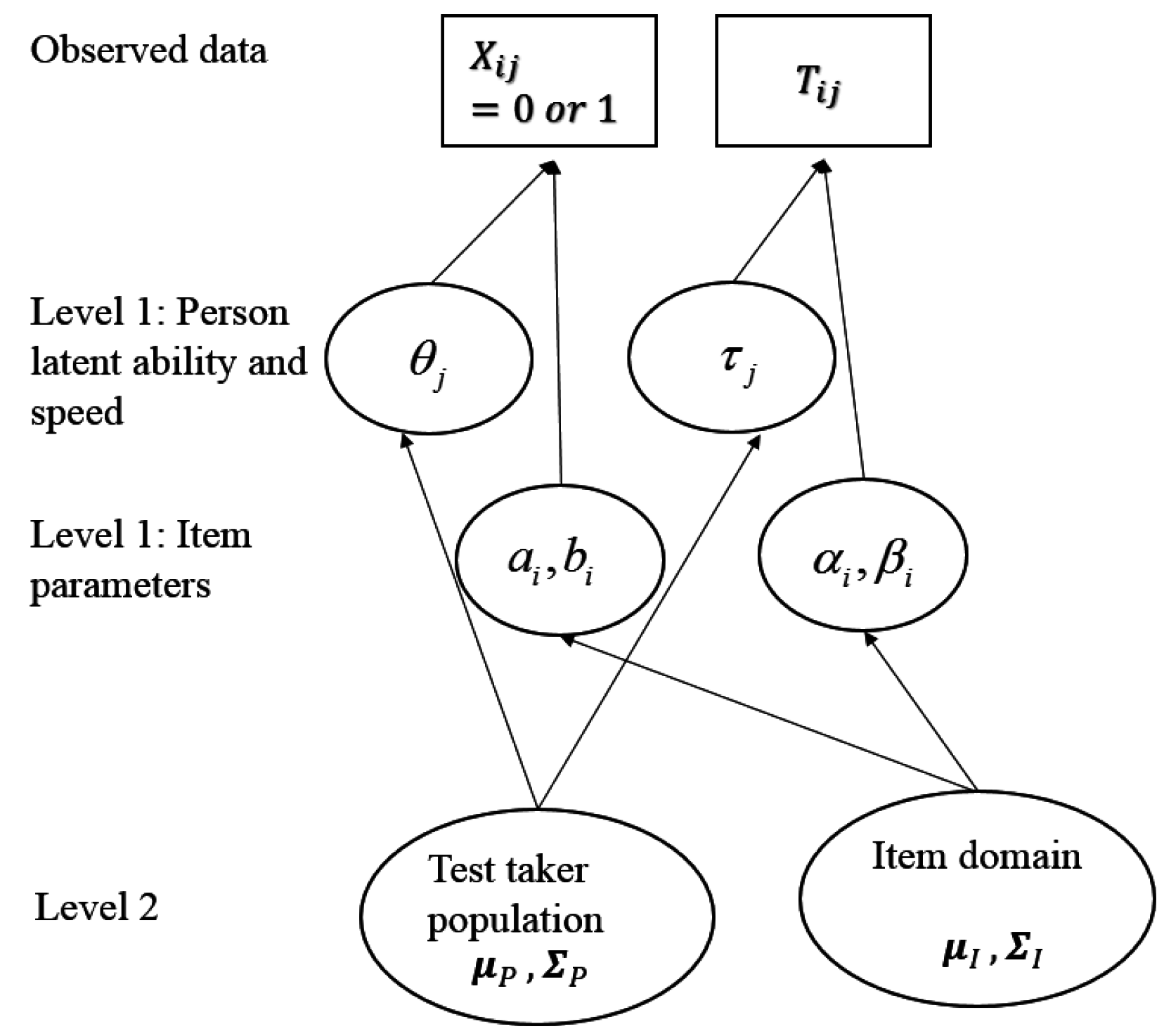
6.2. Hierachical Models

Van der Linden [95] proposed a two-level hierarchical model that jointly models item responses and response times. The first level is for individual examinees and a set of fixed items and the second level is for the population of examinees and items. At the first level, the model assumes that each examinee takes the test with a constant speed and constant ability (a particular location on the individual’s speed–accuracy tradeoff curve), and does not speed up or slow down during the test. Responses and response times are modeled separately by person (ability and speed) and item (difficulty and time-intensity) parameters. For item responses, the model is a three-parameter normal-ogive IRT, where the log odds for a person responding correctly to an item is a function of person ability (${\theta }_j$), item discrimination ($a_i$), item difficulty ($b_i$), and guessing ($c_i$). Actually, any usual IRT models (e.g., the Rasch model, 2PL or 3PL models, or two-parameter or three-parameter normal-ogive models) can be used.

For response time, a lognormal model as is used [96]. This models log response time of a person on an item ($\text{log}{T}_{ij}$) as a function of person speed (${\tau }_j$; which flips the sign, from Thissen’s [94] model, to model speed rather than slowness), item time discrimination (${\alpha }_i$), and item time intensity (${\beta }_i$). Time discrimination reflects how well an item differentiates fast and slow examinees, analogous to item discrimination. The lognormal model for response time has a structure similar to the 2PL model for responses, with both having a latent person parameter (speed or ability), and item parameters that reflect the quality of the item in measuring the intended person parameter. Their differences are that accuracy responses are typically binary and response times are continuous with a natural 0. The lognormal model is similar to Thissen’s [94] response time model in that both model the log of response time, both have latent speed-related person parameters, though of the opposite sign (slowness [94] or speed [95,96]), and both have speed-related item parameters. Their difference is that Thissen [94] models the tradeoff between speed and accuracy by incorporating response parameters in modeling response time. van der Linden [95] assumes for a fixed person, response times are determined only by speed-related parameters and responses are determined only by ability-related parameters. The relationship between speed and ability across people is modeled at the second-level, and is assumed constant across items.13

At the second level, van der Linden [95] respectively models the first-level person and item parameters, which are treated as random, as multivariate normal distributions of mean parameters and variance and covariance parameters. One of the second-level parameters of interest is the correlation between ability and speed in the population of test takers. The path diagram for the model of van der Linden [95] is shown in Figure 1. Appendix A contains mathematical details.

The van der Linden [95] model assumes conditional independence of responses and response times on the same and different items given the person ability and speed. Both Bayesian [99] and frequentist [100] estimation approaches have been proposed. The latter uses marginal maximum likelihood estimation with a Lagrange multiplier test to test hypotheses such as population invariance and the assumption of conditional independence.

Compared to models for only item responses, the estimated person ability in the van der Linden [95] model has less error because more information is incorporated from joint modeling. A simulation study showed that considering response time reduces bias and error in ability estimates, and the degree of improvement increases as the correlation of ability and speed increases, and increases for test takers with extreme abilities [99].

The van der Linden [95] model is a popular and influential joint modeling approach, and has prompted several extensions. One has been to include regression structure to the second-level model for person parameters, enabling studying the effects of covariates on the differences between ability and speed among groups of examinees [101]. Another has been to accommodate Box-Cox transformations on response times, which includes the log transformation as a special case, which makes the model more flexible to meet the normality assumption of the transformed response times for different observed response time distributions [102].

Another extension has been to allow dependence between responses and response times on the same item [103,104]. The van der Linden [95] model assumes conditional independence between responses and response times for an individual, that is, there is an overall correlation between speed and ability, and no additional correlation for a particular item. Another way to state this is that respondents work at a constant rate of speed and accuracy level throughout a test (hence a single ability and speed estimate for each person in the end). However, it seems reasonable that examinees might adjust their position on their own personal speed–accuracy tradeoff curve for a particular item, or they could experience an attention lapse on an item, which would lower accuracy and speed on that item relative to their accuracy and speed on the remaining items. The findings from this literature suggest that such dependencies and therefore violations of the conditional independence assumption do occur.

Molenaar et al. [105] showed that the van der Linden [95] model, which they refer to as the hierarchical crossed random effects model, or hierarchical model, can be simplified to a generalized linear factor model14 with two factors: a factor for categorical responses and a second factor for continuous response times.15 They point out that the hierarchical model includes random item effects, but the generalized linear factor model does not. The advantage of this assumption, and approach, is that generalized linear factor models are relatively well studied, and widely available software such as Mplus and OpenMx can be used to fit the generalized linear factor model (they also provide Mplus and OpenMx syntax). This software makes it quite easy to conduct response time modeling using confirmatory factor analysis (with two correlated factors, one for item responses and a second for item response times), but also to modify the model, for example, to include multiple latent abilities (e.g., for analyzing testlets, or data from several tests together), to add explanatory variables for the person or item parameters (see Section 6.3), or to conduct traditional CFA structural modeling [69] (see Section 5). To assess whether this simplification is appropriate, Molenaar et al. [105] conducted a simulation study by fitting the generalized linear factor model to data generated from the two-parameter version of the hierarchical model, finding that fitting the simplified model did not lead to bias or reduce the efficiency of the item parameter estimates in the conditions studied. (They did not study or report results on person parameter estimates.) The authors also showed that under the generalized linear factor model framework, the responses and response time model could be extended to have a latent class model for the responses or have a nonlinear relationship between speed and ability.

6.3. Cognitive Components

Beginning in the 1970s, there was interest in identifying and measuring the information processing steps associated with solving a problem from a cognitive abilities test, using what came to be known as the cognitive components approach [106]. An example was to take an intelligence test item, create a set of nested subtasks based on that item, then to subtract partial from full task performance times to estimate the duration of processing stages within that item. Sternberg [107] implemented this approach using multiple regression with response time for the full and partial tasks as the dependent variable, and a design matrix indicating the presence (or not) of a processing stage for a particular task or subtask as the predictor variables. More generally, and whether or not items are full and partially embedded subtasks, the design matrix is an item-by- attribute matrix (commonly referred to as a Q matrix), and one models item responses based on that matrix, in a process now known as cognitive diagnostic modeling (CDM) [108,109,110]. However, CDMs are most often designed to model responses rather than response times. An early IRT version of this general concept was the linear logistic test model (LLTM) [47]. The LLTM is a 1PL, but instead of modeling item responses with an item difficulty parameter, b_i, for each item i, it models item responses with a set of attribute difficulty parameters, d_k, which do or do not come into play depending on the attributes called for on a particular item as represented in the Q matrix q_ik. Thus in LLTM, b_i is substituted for as

$$b_i={\displaystyle \sum _k^K{q}_{ik}{d}_k}.$$

A number of studies have applied this model to the analysis of items from cognitive tests [111], such as figural matrices [112], and reading comprehension [113]. The general approach is to conduct two separate analyses. In the first, response (accuracy) data are analyzed, using either LLTM or multiple regression; in the second, response time (or log response time) is regressed on the same design (Q-matrix) variables to get estimates of the duration of processing stages. A benefit of this approach is that enables the explicit identification of the cognitive processes underlying problem difficulty, which is useful for construct validity, and for enabling automatic, on-the-fly item generation [111].

A limitation of the two-step approach is that it fails to model the relationship between responses and response times [114]. Klien Entink et al. [114] proposed to marry an LLTM approach with the hierarchical modeling approach, as discussed in Section 6.2 [95]. They also employed a full Bayesian framework using Markov Chain Monte Carlo methods to estimate the model. Although in the end their findings [114] were not too dissimilar to ones obtained earlier using a two-step approach [115], Klein Entink et al. [114] were able to provide a more complete picture of the effects of design features on accuracy and response time. Thus, their approach serves as a model for jointly analyzing accuracy and response time data on complex mental ability tests. The value of this hierarchical approach was later demonstrated in a study examining the relationship between reasoning ability and reasoning speed [29].

6.4. Assessing Ability and Speed in Power Tests with Observations from Time-Limit Tests

In real-world standardized testing, from a construct validity perspective, it is often desired to measure ability (level) with a power test. However, for practical reasons, or for fairness, time limits are almost always imposed. This makes a pure power test an unobtainable ideal, with a time-limit test its practical substitute. To assess ability level as it would have been measured from a pure power test but based on responses from a time-limit test, Lee & Ying [116] proposed a mixture cure-rate model, combining IRT with a survival time model (from survival analysis). Survival analysis models time-to-event data (such as time to death, or completion time, or, in this case, time to response), and allows for censored data, data not fully observed (e.g., time-to-death samples with still living subjects, or in this case, samples with item responses with processing times where processing was not complete to the point of getting a correct answer). Constant censored time (C) could be imposed (e.g., item-level time limits, see Section 4.3.2), or even item-specific censored time (C_i), but in most tests (specifically, time-limit tests) it is not, and so the censoring variable C is assumed to be examinee-item specific, that is, as C_ij.

In their model, power time ($T_{ij}^{*}$) is defined as the time it would take an examinee to respond if time were unlimited, and a dichotomous response variable indicates whether the examinee would be able to answer an item correctly given unlimited time (${\eta }_{ij}=1$ if they would, 0 otherwise), based on their ability and item difficulty. There are three possibilities:

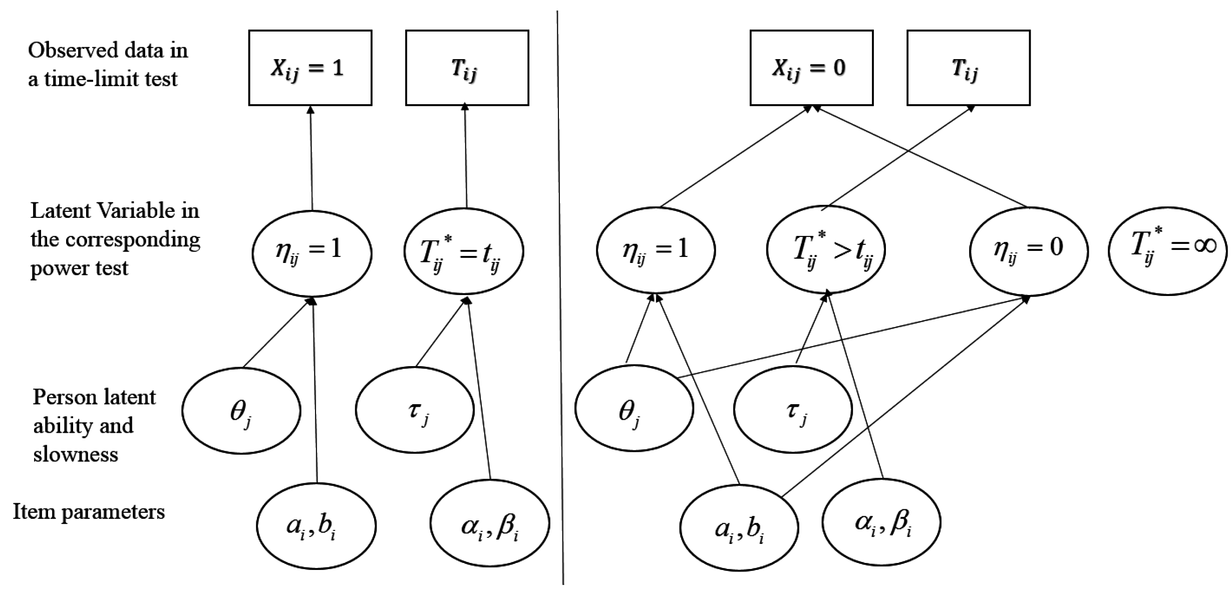
• If an examinee responds correctly within the time limit, then it is assumed that the examinee would get it correct in unlimited time (${\eta }_{ij}=1$), and power time ($T_{ij}^{*}$) for that item is the same as observed time (t_ij) for that item (the model assumes no guessing); log power time (log[$T_{ij}^{*}$]) is a function of person slowness (${\tau }_j$), item time-intensity (${\beta }_i$), a random variable (${\epsilon }_{ij}$) with mean 0, and a scale parameter (${\alpha }_i$, analogous to the time discrimination parameter in [98]).
• If an examinee responds incorrectly within the time limit, then they might or might not have gotten it correct with unlimited time, depending on ability and item difficulty. Censoring time is the time an examinee chooses to give up working on an item and is equal to observed time t_ij:

  • For those examinees expected to answer correctly with unlimited time (${\eta }_{ij}=1$), log power time (log[$T_{ij}^{*}$])) is modeled as in the first case and t_ij is a lower bound of power time;
  • For those not expected to answer correctly with unlimited time (${\eta }_{ij}=0$), power time is infinity.

The path diagram for this mixture cure rate model is shown in Figure 2. Mathematical details are provided in Appendix A.

The authors point out that the model is general in that it includes IRT modeling of power tests and RT modeling of speeded tests as special cases. The model assumes that power time (how long it would take to answer an item correctly) and censoring time (how long an examinee chooses to work on a problem before abandoning a solution attempt) are independent. The authors [116] described a marginal maximum likelihood estimation approach, evaluate the model in several simulation studies, and argue for several benefits to their model, particularly its ability to distinguish low proficiency from lack of time in ability estimation on time-limit tests. They also point out current limitations, such as its ability to handle getting a correct answer through guessing. They discuss possible extensions including Bayesian estimation methods and allowing for dependent censoring (e.g., choosing to persist or not depending on power time for an item).

6.5. Diffusion-Based IRT models

In a previous section (Section 5.2), we listed the diffusion model as an example of an evidence accumulation process model from cognitive psychology, developed to explain response processes on memory retrieval and decision tasks. Although prior research [69,83] showed how model parameters could be used to elucidate individual and group differences, the diffusion model was not a psychometric item response model per se.

Tuerlinckx & De Boeck [70] showed how the diffusion model could be directly expressed as a 2PL IRT model. Fitting the traditional diffusion model in cognitive psychology experiments involves an examinee taking a large number of items (i.e., trials) with item-feature counter balancing, so that items are considered interchangeable, and specific item effects are not modeled. This is different from IRT models. To connect the diffusion model and IRT models, the authors [70] made item effects explicit. Specifically, for person j and item i, they decomposed the drift rate into a person component and an item component, that is ${\upsilon }_{ij}={\theta }_j-b_i$. They showed that if the diffusion process is unbiased (i.e., the process starts in the middle between boundaries, that is, at $a_i/2$) and assuming the variance of drift rate equals 1 for model identification, the probability of choosing the upper criterion is the same as the 2PL IRT model. The boundary parameter $a_i$ in the diffusion model is the discrimination parameter ($a_i$) in the 2PL model, ${\theta }_j$ is interpreted as person ability, and $b_i$ is item difficulty. They also demonstrate their model with a unidimensional pairwise preference personality test.

Van der Maas et al. [71] extended and altered the Tuerlinckx-De Boeck [70] model by first, redefining drift rate from a difference to a quotient function (hence, Q-diffusion), the ratio of person ability to item difficulty, ${\upsilon }_{ij}={\theta }_j/b_i$. The reason they propose quotients over differences for drift rate is so that abilities and item difficulties can be expressed positively, with a natural zero point (“the positive ability model”); they provide the metaphor with speed = power/force, for drift rate = ability/difficulty. Second, they decompose boundary separation into the ratio of a person component (response cautiousness) and an item component (time pressure) ($a_{ij}={\gamma }_j/d_i$). Thus, a person’s response criterion is reached (i.e., the person decides to respond, reaches a boundary) more slowly when the person is a more cautious person, or there is little time pressure. A less cautious person, or more time pressure leads to deciding more quickly.

Van der Maas et al. [71] also proposed a D-diffusion IRT model (D for difference) that retains the Tuerlinckx-De Boeck [70] difference definition of drift rate. Like Tuerlinckx–De Boeck [70] they see the appropriateness of this model for measuring personality, particularly, based on a trait preference or a binary (true-false) decision. Decision making is fastest for those high or low on the trait (a “distance-difficulty” hypothesis [31,117]), and increasing the time limit will make low (high) trait respondents less (more) likely to say yes. A marginal maximum likelihood estimation approach for the D- and Q-diffusion models has been implemented in an R package, diffIRT [118].

7. Fast vs. Slow Responding = Fast vs. Slow Thinking?

Dual process theory in psychology refers to the notion that there are two qualitatively different kinds of thinking, one fast, automatic, and intuitive and the other slow, controlled, and deliberate [119]. For example, experts (e.g., chess masters, drivers, mathematicians, readers) see a pattern (e.g., board configuration, traffic pattern, equation, letters on a page) and automatically know the solution (e.g., its interpretation, what to do), whereas novices deliberatively think it through, slowly, step by step. If experts quickly see a solution when novices struggle to work it out, it might seem that speed and ability should be highly correlated. However, experts sometimes make mistakes and novices sometimes work out the answer, and so it might be more appropriate to believe that regardless of ability level, individuals may process information differently on different occasions. This has been referred to as System 1 (fast, intuitive, emotional, “jumping to conclusions”) and System 2 (slow, deliberate, logical, methodical) processing [120], with the former responsible for some thinking shortcuts (heuristics), but also cognitive biases (e.g., confirmation bias, fundamental attribution error). Invoking System 1 vs. System 2 processing also does not necessarily seem simply to be a matter of expertise as cognitively high ability individuals are often just as susceptible to many cognitive biases, such as overconfidence and false consensus, as low ability individuals are (e.g., [121,122]).

This raises an interesting question of whether response time analysis might capture different processing (e.g., System 1 vs. System 2) within an individual. There already may be a hint of this in the “worst performance rule (WPR)” [123], which is based on a finding that the average response time from one’s slowest responses (or, say, the 90th percentile of response times for an individual) is more highly correlated with cognitive ability than is one’s mean response time across all responses [124]. The WPR could result from the comparison between uninformative rapid guessing responses vs. informative full processing responses [125]. Or the WPR could result from high ability individuals less likely to mind wander during processing [126,127]. The mind-wandering hypothesis may be implicated in the ex-Gaussian research (see Section 5.1), which found that the waiting time (exponential) component of response time distributions, and not the processing time (Gaussian) components, was the component that correlated highest with cognitive ability [69].

Partchev and De Boeck [128] explored the idea that there may be qualitatively different types of processing, and consequently different abilities invoked within a putatively single-construct test, in the following way. They dichotomized each individual’s response times (from a verbal analogies and a progressive matrices test) into a fast vs. slow category, based either on the person’s median or on the median response time to each item, yielding fast-correct, fast-incorrect, slow-correct, and slow-incorrect response categories. They then fit a 1PL IRTree model [129], and found that three different latent traits were required to fit the data: speed, slow intelligence, and fast intelligence. They also found that although fast and slow intelligence were highly correlated, they were distinguishable. A follow-up effort [130] extended the methodology to a 2PL IRTree, which enabled investigating which kind of response speed tends to contain more information about intelligence. With this methodology they did not find a distinction between fast and slow intelligence, suggesting that there was a common ability running through fast and slow responses. They also did not find support for the WPR in their data, using either the original binning methodology or their IRTree methodology, suggesting that speed on elementary cognitive tasks, as investigated in much of the cognitive psychology literature, and on speeded tasks in the abilities literature, is not the same as response speed on complex ability tests. They also pointed out that their methodology was potentially useful for addressing questions about processing strategies on items (e.g., fast correct answers could indicate one happening upon an efficient strategy for that item). Coomans et al. [131] outline a different approach to address this issue, and point out that such investigations open the door to collaborations between psychometrics and cognitive psychology.

8. Other Uses of Response Time

This article focused on measuring ability and response time, but it is useful to point out that many of the approaches discussed here may also be used for other applications in testing as well. These include assessing examinee motivation levels, particularly for low stakes tests [132,133,134], evaluating strategy use, for example by differences in response times for subgroups employing different problem solving strategies [130,135], or even the same individual employing different strategies at different points in the test [136], and evaluating cultural differences in pacing and time management during test taking [137]. Other applications include detecting cheating [97], assembling parallel forms [138], and item selection in adaptive testing [139,140], which may be particularly important for ensuring score comparability16 across sets of items that might be similar in difficulty but differ in their time intensity [142,143]. Finally, although the applications here focused on response time for cognitive tests, another application only briefly mentioned here (Section 6.4) is to model response time on personality and attitude assessments [31,144,145]. The general idea is that response time in a choice task, such as a forced-choice personality item (e.g., “which is more true of you, you are pessimistic or optimistic?”, or “are you outgoing or reserved?”), can be modeled with approaches used in cognitive tasks, such as a diffusion model [70,71,118], or a simpler 1PL model [6], in which the item difficulty pertains to the difficulty of the choice one makes in deciding whether a word or statement describes oneself appropriately or not.

9. Discussion

Response time has been a topic of discussion in ability testing since its beginnings. However, the transition to computer-based testing, which began in the 1970s, is just now becoming commonplace in large scale assessments such as PISA and NAEP, and is having an effect of a resurgence of interest in the topic. In addition, there have been significant developments in psychometrics enabling more sophisticated approaches to measuring speed and ability, and more accessible software for conducting such analyses. There is every indication that the topic of measuring response time, for its own sake, to improve the quality of ability measurement, or for additional applications, such as form assembly and cheating detection will continue to grow in popularity.

In this article, we focused on approaches and implications for measuring response time in the context of ability measurement. We pointed out that response time has always been an important topic in ability measurement, and that a significant and important distinction is between speed and level abilities which are typically measured by speeded and power tests, respectively. We have always recognized that a pure speed and pure power test is a theoretical concept, and that in practical applications there will likely always be some kind of time limit placed on a test. Not only is this necessary for logistical and cost containment reasons, but a truly time unlimited test probably measures constructs that are not the ones we typically intend to measure. As an example, consider that on a test to recall names of students from one’s high school class, examinees can continue to recall additional names even after 9 h of testing [146]. For such a task, the construct changes at some point from memory recall to problem solving.

Ability frameworks [19] identify major factors that can be classified as primarily level (general cognitive ability, fluid ability, crystallized ability, spatial ability, learning and memory) or as primarily speed (general retrieval ability, general speediness, processing speed). However, there also have been proposals for correlated aspects of level abilities such as speed and level reasoning or verbal comprehension. The new psychometric tools available now promise to provide better insights into the nature of this distinction.

We also discussed several new methods that can be used to provide greater insight into the speed and level aspects of cognitive ability, and speed–accuracy tradeoff decisions. These include item-level time limits, the use of feedback (e.g., CUSUMs), and explicit scoring rules that combine speed and accuracy information (e.g., count down timing).

However, it seems that the major development over the past decade or so has been in the development of more sophisticated psychometric models that combine speed and ability measurement, account for speed–accuracy tradeoff, and allow for distinctions between response times on different kinds of items, and on items responded to correctly and incorrectly. The application of these models and tools is likely to advance both the science of human abilities, and their measurement for real-world use.

References

1. Jensen, A.R. Galton’s Legacy to Research on Intelligence. J. Biosoc. Sci. 2002, 34, 145–172. [Google Scholar] [CrossRef] [PubMed]
2. Spearman, C. General Intelligence, Objectively Determined and Measured. Am. J. Psychol. 1904, 15, 201–292. [Google Scholar] [CrossRef]
3. Goldhammer, F. Measuring ability, speed, or both? Challenges, psychometric solutions, and what can be gained from experimental control. Meas. Interdiscip. Res. Perspect. 2015, 13, 133–164. [Google Scholar] [CrossRef] [PubMed]
4. Lee, Y.-H.; Chen, H. A review of recent response-time analyses in educational testing. Psychol. Test Assess. Model. 2011, 53, 359–379. [Google Scholar]
5. Schnipke, D.L.; Scrams, D.J. Exploring issues of examinee behavior: Insights gained from response-time analyses. In Computer-Based Testing: Building the Foundation for Future Assessments; Mills, C.N., Potenza, M., Fremer, J.J., Ward, W., Eds.; Lawrence Erlbaum Associates: Hillsdale, NJ, USA, 2002; pp. 237–266. [Google Scholar]
6. Van der Linden, W.J. Conceptual issues in response-time modeling. J. Educ. Meas. 2009, 46, 247–272. [Google Scholar] [CrossRef]
7. Thorndike, E.L.; Bregman, E.O.; Cobb, M.V.; Woodyard, E.; The Staff of the Division of Psychology of the Institute of Educational Research at Teachers College, Columbia University. The Measurement of Intelligence; Teachers College, Columbia University: New York, NY, USA, 1926; Available online: https://archive.org/details/measurementofint00thoruoft (accessed on 10 September 2016).
8. Cronbach, L.J.; Warrington, W.G. Time-limit tests: Estimating their reliability and degree of speeding. Psychometrika 1951, 6, 167–188. [Google Scholar] [CrossRef]
9. Helmstadter, G.C.; Ortmeyer, D.H. Some techniques for determining the relative magnitude of speed and power components of a test. Educ. Psychol. Meas. 1953, 8, 280–287. [Google Scholar] [CrossRef]
10. Swineford, F. The Test Analysis Manual; ETS SR 74-06; Educational Testing Service: Princeton, NJ, USA, 1974. [Google Scholar]
11. Rindler, S.E. Pitfalls in assessing test speededness. J. Educ. Meas. 1979, 16, 261–270. [Google Scholar] [CrossRef]
12. Bridgeman, B.; Trapani, C.; Curley, E. Impact of fewer questions per section on SAT I scores. J. Educ. Meas. 2004, 41, 291–310. [Google Scholar] [CrossRef]
13. Davidson, W.M.; Carroll, J.B. Speed and level components of time limit scores: A factor analysis. Educ. Psychol. Meas. 1945, 5, 411–427. [Google Scholar]
14. Dwyer, P.S. The determination of the factor loadings of a given test from the known factor loadings of other tests. Psychometrika 1937, 2, 173–178. [Google Scholar] [CrossRef]
15. Neisser, U. Cognitive Psychology; Prentice-Hall: Englewood Cliffs, NJ, USA, 1967. [Google Scholar]
16. Shepard, R.; Metzler, J. Mental rotation of three-dimensional objects. Science 1971, 171, 701–703. [Google Scholar] [CrossRef] [PubMed]
17. Lohman, D.F. Spatial Ability: Individual Differences in Speed and Level; Technical Report No. 9; Stanford University, Aptitude Research Project, School of Education (NTIS NO. AD-A075 973): Stanford, CA, USA, 1979. [Google Scholar]
18. Kyllonen, P.C.; Tirre, W.C.; Christal, R.E. Knowledge and processing speed as determinants of associative learning. J. Exp. Psychol. Gen. 1991, 120, 89–108. [Google Scholar] [CrossRef]
19. Carroll, J.B. Human Cognitive Abilities: A Survey of Factor Analytic Studies; Cambridge University Press: New York, NY, USA, 1993. [Google Scholar]
20. Cattell, R.B. Abilities: Their Structure, Growth, and Action; Houghton Mifflin: Boston, MA, USA, 1971. [Google Scholar]
21. Horn, J.L.; Cattell, R.B. Refinement and test of the theory of fluid and crystallized general intelligences. J. Educ. Psychol. 1966, 57, 253–270. [Google Scholar] [CrossRef] [PubMed]
22. Kyllonen, P.C. Human cognitive abilities: Their organization, development, and use. In Handbook of Educational Psychology, 3rd ed.; Routledge: New York, NY, USA, 2015; pp. 121–134. [Google Scholar]
23. McGrew, K. CHC theory and the human cognitive abilities project: Standing on the shoulders of the giants of psychometric intelligence research. Intelligence 2009, 37, 1–10. [Google Scholar] [CrossRef]
24. Schneider, W.J.; McGrew, K. The Cattell-Horn-Carroll model of intelligence. In Contemporary Intellectual Assessment: Theories, Tests, and Issues, 3rd ed.; Flanagan, D., Harrison, P., Eds.; Guilford: New York, NY, USA, 2012; pp. 99–144. [Google Scholar]
25. Danthiir, V.; Wilhelm, O.; Roberts, R.D. Further evidence for a multifaceted model of mental speed: Factor structure and validity of computerized measures. Learn. Individ. Differ. 2012, 22, 324–335. [Google Scholar] [CrossRef]
26. Roberts, R.D.; Stankov, L. Individual differences in speed of mental processing and human cognitive abilities: Towards a taxonomic model. Learn. Individ. Differ. 1999, 11, 1–120. [Google Scholar] [CrossRef]
27. Sheppard, L.D.; Vernon, P.A. Intelligence and speed of information-processing: A review of 50 years of research. Personal. Individ. Differ. 2008, 44, 535–551. [Google Scholar] [CrossRef]
28. Dodonova, Y.A.; Dodonov, Y.S. Faster on easy items, more accurate on difficult ones: Cognitive ability and performance on a task of varying difficulty. Intelligence 2013, 41, 1–10. [Google Scholar] [CrossRef]
29. Goldhammer, F.; Entink, R.H.K. Speed of reasoning and its relation to reasoning ability. Intelligence 2011, 39, 108–119. [Google Scholar] [CrossRef]
30. Wilhelm, O.; Schulze, R. The relation of speeded and unspeeded reasoning with mental speed. Intelligence 2002, 30, 537–554. [Google Scholar] [CrossRef]
31. Ferrando, P.J.; Lorenzo-Seva, U. An item-response model incorporating response time data in binary personality items. Appl. Psychol. Meas. 2007, 31, 525–543. [Google Scholar] [CrossRef]
32. White, P.O. Individual differences in speed, accuracy, and persistence: A mathematical model of problem solving. In A Model for Intelligence; Eysenck, H.J., Ed.; Springer: Berlin, Germany, 1973; pp. 44–90. [Google Scholar]
33. Heitz, R.P. The speed–accuracy tradeoff: History physiology, methodology, and behavior. Front. Neurosci. 2014, 8, 150. [Google Scholar] [CrossRef] [PubMed]
34. Henmon, V. The relation of the time of a judgment to its accuracy. Psychol. Rev. 1911, 18, 186–201. [Google Scholar] [CrossRef]
35. Bridgeman, B.; Cline, F.; Hessinger, J. Effect of Extra Time on GRE® Quantitative and Verbal Scores; ETS RR-03-13; Educational Testing Service: Princeton, NJ, USA, 2003. [Google Scholar]
36. Evans, F.R. A Study of the Relationships among Speed and Power Aptitude Test Score, and Ethnic Identity; ETS RR 80-22; Educational Testing Service: Princeton, NJ, USA, 1980. [Google Scholar]
37. Wild, C.L.; Durso, R.; Rubin, D.B. Effects of increased test-taking time on test scores by ethnic group, years out of school, and sex. J. Educ. Meas. 1982, 19, 19–28. [Google Scholar] [CrossRef]
38. Lohman, D.F. The effect of speed–accuracy tradeoff on sex differences in mental rotation. Percept. Psychophys. 1986, 39, 427–436. [Google Scholar] [CrossRef] [PubMed]
39. Sternberg, S. The discovery of processing stages: Extensions of Donders’ method. Acta Psychol. 1969, 30, 276–315. [Google Scholar] [CrossRef]
40. Shiffrin, R.M.; Schneider, W. Controlled and automatic human information processing: II. Perceptual learning, automatic attending, and a general theory. Psychol. Rev. 1977, 84, 127–190. [Google Scholar] [CrossRef]
41. Wickegren, W. Speed–accuracy tradeoff and information processing dynamics. Acta Psychol. 1977, 41, 67–85. [Google Scholar] [CrossRef]
42. Lohman, D.F. Individual differences in errors and latencies on cognitive tasks. Learn. Individ. Differ. 1989, 1, 179–202. [Google Scholar] [CrossRef]
43. Reed, A.V. List length and the time course of recognition in human memory. Mem. Cogn. 1976, 4, 16–30. [Google Scholar] [CrossRef] [PubMed]
44. Wright, D.E.; Dennis, I. Exploiting the speed-accuracy trade-off. In Learning and Individual Differences: Process, Trait, and Content Determinants; Ackerman, P.L., Kyllonen, P.C., Roberts, R.D., Eds.; American Psychological Association: Washington, DC, USA, 1999. [Google Scholar]
45. Irvine, S. Computerised Test Generation for Cross-National Military Recruitment; IOS Press: Amsterdam, The Netherlands, 2014. [Google Scholar]
46. Lewis, C. Expected response functions. In Essays on Item Response Theory; Boomsma, A., van Duijn, M.A.J., Snijders, T.A.B., Eds.; Springer: New York, NY, USA, 2001; Volume 157, pp. 163–171. [Google Scholar]
47. Fischer, G.H. The linear logistic test model as an instrument in educational research. Acta Psychol. 1973, 37, 359–374. [Google Scholar] [CrossRef]
48. Irvine, S.; Kyllonen, P.C. Item Generation for Test Development; Erlbaum: Mahwah, NJ, USA, 2002. [Google Scholar]
49. Gierl, M.J.; Haladyna, T. Automatic Item Generation: Theory and Practice; Routledge: New York, NY, USA, 2013. [Google Scholar]
50. Beilock, S.L.; Bertenthal, B.I.; Hoerger, M.; Carr, T.H. When does haste make waste? Speed–accuracy tradeoff, skill level, and the tools of the trade. J. Exp. Psychol. Appl. 2008, 14, 340–352. [Google Scholar] [CrossRef] [PubMed]
51. Lohman, D.F. Estimating individual differences in information processing using speed-accuracy models. In Abilities, Motivation, Methodology: The Minnesota Symposium on Learning and Individual Differences; Kanfer, R., Ackerman, P.L., Cudeck, R., Eds.; Psychology Press: New York, NY, USA, 1990; pp. 119–163. [Google Scholar]
52. Evans, J.S.B.T.; Wright, D.E. The Properties of Fixed-Time Tests: A Simulation Study; Technical Report 3-1993, Army Personnel Research Establishment; Human Assessment Laboratory, University of Plymouth: Plymouth, UK, 1993. [Google Scholar]
53. Partchev, I.; De Boeck, P.; Steyer, R. How much power and speed is measured in this test? Assessment 2013, 20, 242–252. [Google Scholar] [CrossRef] [PubMed]
54. Birnbaum, A. Some latent trait models and their use in inferring an examinee’s ability. In Statistical Theories of Mental Test Scores; Lord, F.M., Novick, M.R., Eds.; Addison-Wesley: Reading, MA, USA, 1968. [Google Scholar]
55. Way, W.D.; Gawlick, L.A.; Eignor, D.R. Scoring Alternatives for Incomplete Computerized Adaptive Tests; Research Report No. RR-01-20; Educational Testing Service: Princeton, NJ, USA, 2001. [Google Scholar]
56. Weeks, J.P.; Kyllonen, P.C.; Bertling, M.; Bertling, J.P. General Fluid/Inductive Reasoning Battery for a High-Ability Population; Unpublished manuscript; Educational Testing Service: Princton, NJ, USA, 2016. [Google Scholar]
57. Wright, D.E. BARB and the Measurement of Individual Differences, Departing from Traditional Models. In Proceedings of the 35th International Military Testing Association Conference, Williamsburg, VA, USA, 15–18 November 1993; pp. 391–395.
58. Ali, U.S.; Rijn, P.W. Psychometric quality of scenario-based tasks to measure learning outcomes. In Proceedings of the 2nd International Conference for Assessment and Evaluation, Riyadh, Saudi Arabia, 1–3 December 2015; Available online: http://ica.qiyas.sa/Presentations/Usama%20Ali.pdf (accessed on 10 September 2016).
59. Maris, G.; van der Maas, H. Speed-accuracy response models: Scoring rules based on response time and accuracy. Psychometrika 2012, 77, 615–633. [Google Scholar] [CrossRef]
60. Dennis, I.; Evans, J.S.B.T. The speed-error trade-off problem in psychometric testing. Br. J. Psychol. 1996, 87, 105–129. [Google Scholar] [CrossRef]
61. Van der Maas, H.L.J.; Wagenmakers, E.-J. A psychometric analysis of chess expertise. Am. J. Psychol. 2005, 118, 29–60. [Google Scholar] [PubMed]
62. Luce, R.D.; Bush, R.R.; Galanter, E. Handbook of Mathematical Psychology. Vol 1; John Wiley & Sons: New York, NY, USA, 1963. [Google Scholar]
63. Newell, A. You can’t play 20 questions with nature and win. In Visual Information Processing; Chase, W.G., Ed.; Academic Press: New York, NY, USA, 1973. [Google Scholar]
64. Luce, R.D. Response Times; Oxford University Press: New York, NY, USA, 1986. [Google Scholar]
65. Hunt, E.B.; Davidson, J.; Lansman, M. Individual differences in long-term memory access. Mem. Cogn. 1981, 9, 599–608. [Google Scholar] [CrossRef]
66. Kyllonen, P.C. Aptitude testing inspired by information processing: A test of the four-sources model. J. Gen. Psychol. 1993, 120, 375–405. [Google Scholar] [CrossRef]
67. Faust, M.E.; Balota, D.A.; Spieler, D.H.; Ferraro, F.R. Individual differences in information processing rate and amount: Implications for group differences in response latency. Psychol. Bull. 1999, 125, 777–799. [Google Scholar] [CrossRef] [PubMed]
68. Pieters, L.P.M.; van der Ven, A.H.G.S. Precision, speed, and distraction in time limit-tests. Appl. Psychol. Meas. 1982, 6, 93–109. [Google Scholar] [CrossRef]
69. Schmiedek, F.; Oberauer, K.; Wilhelm, O.; Süß, H.M.; Wittmann, W.W. Individual differences in components of reaction time distributions and their relations to working memory and intelligence. J. Exp. Psychol. Gen. 2007, 136, 414–429. [Google Scholar] [CrossRef] [PubMed]
70. Tuerlinckx, F.; De Boeck, P. Two interpretations of the discrimination parameter. Psychometrika 2005, 70, 629–650. [Google Scholar] [CrossRef]
71. Van der Maas, H.L.; Molenaar, D.; Maris, G.; Kievit, R.A.; Borsboom, D. Cognitive psychology meets psychometric theory: On the relation between process models for decision making and latent variable models for individual differences. Psychol. Rev. 2011, 118, 339–177. [Google Scholar] [CrossRef] [PubMed]
72. Underwood, B.J. Individual differences as a crucible in theory construction. Am. Psychol. 1975, 30, 128–134. [Google Scholar] [CrossRef]
73. Murre, J.M.J.; Chessa, A.G. Power laws from individual differences in learning and forgetting: mathematical analyses. Psychon. Bull. Rev. 2011, 18, 592–597. [Google Scholar] [CrossRef] [PubMed]
74. Newell, A.; Rosenbloom, P.S. Mechanisms of skill acquisition and the law of practice. In Cognitive Skills and Their Acquisition; Anderson, J.R., Ed.; Erlbaum: Hillsdale, NJ, USA, 1981; pp. 1–55. [Google Scholar]
75. Heathcote, A.; Brown, S.; Mewhort, D.J. The power law repealed: the case for an exponential law of practice. Psychon. Bull. Rev. 2000, 7, 185–207. [Google Scholar] [CrossRef] [PubMed]
76. Furneaux, W.D. Intellectual abilities and problem solving behavior. In Handbook of Abnormal Psychology; Eysenck, H.J., Ed.; Pitman Medical: London, UK, 1960; pp. 167–192. [Google Scholar]
77. Lacouture, Y.; Cousineau, D. How to use MATLAB to fit the ex-Gaussian and other probability functions to a distribution of response times. Tutor. Quant. Methods Psychol. 2008, 4, 35–45. [Google Scholar] [CrossRef]
78. R Core Team R: A Language and Environment for Statistical Computing; R Foundation for Statistical Computing: Vienna, Austria, 2014; Available online: http://www.R-project.org/ (accessed on 10 September 2016).
79. Massidda, D. Retimes: Reaction Time Analysis; R Package Version 0.1-2; R Foundation for Statistical Computing: Vienna, Austria, 2015. [Google Scholar]
80. Ratcliff, R. A theory of memory retrieval. Psychol. Rev. 1978, 85, 59–108. [Google Scholar] [CrossRef]
81. Ratcliff, R.; Smith, P.L.; Brown, S.D.; McKoon, G. Diffusion decision model: Current issues and history. Trends Cogn. Sci. 2016, 20, 260–281. [Google Scholar] [CrossRef] [PubMed]
82. Donkin, C.; Brown, S.; Heathcote, A.; Wagenmakers, E.J. Diffusion versus linear ballistic accumulation: Different models but the same conclusions about psychological processes? Psychon. Bull. Rev. 2011, 18, 61–69. [Google Scholar] [CrossRef] [PubMed]
83. Ratcliff, R.; Thapar, A.; Gomez, P.; McKoon, G. A diffusion model analysis of the effects of aging in the lexical-decision task. Psychol. Aging 2004, 19, 278–289. [Google Scholar] [CrossRef] [PubMed]
84. Ratcliff, R.; Tuerlinckx, F. Estimating parameters of the diffusion model: Approaches to dealing with contaminant reaction times and parameter variability. Psychon. Bull. Rev. 2002, 9, 438–481. [Google Scholar] [CrossRef] [PubMed]
85. Ratcliff, R.; Childers, C. Individual differences and fitting methods for the two-choice diffusion model of decision making. Decision 2015, 4, 237–279. [Google Scholar] [CrossRef] [PubMed]
86. Held, J.D.; Carretta, T.R. Evaluation of Tests of Processing Speed, Spatial Ability, and Working Memory for Use in Military Occupational Classification; Technical Report NPRST-TR-14-1 (ADA589951); Navy Personnel Research, Studies, and Technology (Navy Personnel Command): Millington, TN, USA, 2013. [Google Scholar]
87. Caplin, A.; Martin, D. The dual-process drift diffusion model: Evidence from response times. Econ. Inq. 2016, 54, 1274–1282. [Google Scholar] [CrossRef]
88. Lord, F.M.; Novick, M.R. Statistical Theories of Mental Test Scores; Addison-Wesley: Reading, MA, USA, 1968. [Google Scholar]
89. Roskam, E.E. Toward a psychometric theory of intelligence. In Progress in Mathematical Psychology; Roskam, E.E., Suck, R., Eds.; North Holland: Amsterdam, The Netherlands, 1987; pp. 151–171. [Google Scholar]
90. Roskam, E.E. Models for speed and time-limit tests. In Handbook of Modern Item Response Theory; van der Linden, W.J., Hambleton, R.K., Eds.; Springer: New York, NY, USA, 1997; pp. 187–208. [Google Scholar]
91. Verhelst, N.D.; Verstralen, H.H.F.M.; Jansen, M.G.H. A logistic model for time-limit tests. In Handbook of Modern Item Response Theory; van der Linden, W.J., Hambleton, R.K., Eds.; Springer: New York, NY, USA, 1997; pp. 169–186. [Google Scholar]
92. Wang, T.; Hanson, B.A. Development and calibration of an item response model that incorporates response time. Appl. Psychol. Meas. 2005, 29, 323–339. [Google Scholar] [CrossRef]
93. Gaviria, J.-L. Increase in precision when estimating parameters in computer assisted testing using response times. Qual. Quant. 2005, 39, 45–69. [Google Scholar] [CrossRef]
94. Thissen, D. Timed testing: An approach using item response theory. In New Horizons in Testing: Latent Trait Test Theory and Computerized Adaptive Testing; Weiss, D.J., Ed.; Academic Press: New York, NY, USA, 1983; pp. 179–203. [Google Scholar]
95. Van der Linden, W.J. A hierarchical framework for modeling speed and accuracy on test items. Psychometrika 2007, 72, 287–308. [Google Scholar] [CrossRef]
96. Van der Linden, W.J. A lognormal model for response times on test items. J. Educ. Behav. Stat. 2006, 31, 181–204. [Google Scholar] [CrossRef]
97. Van der Linden, W.; Guo, F. Bayesian procedures for identifying aberrant response time patterns in adaptive testing. Psychometrika 2008, 73, 365–384. [Google Scholar] [CrossRef]
98. Van der Linden, W.J.; Breithaupt, K.; Chuah, S.C.; Zhang, Y. Detecting differential speededness in multistage testing. J. Educ. Meas. 2007, 44, 117–130. [Google Scholar] [CrossRef]
99. Van der Linden, W.J.; Klein Entink, R.H.; Fox, J.-P. IRT parameter estimation with response time as collateral information. Appl. Psychol. Meas. 2010, 34, 327–347. [Google Scholar] [CrossRef]
100. Glas, C.A.; van der Linden, W.J. Marginal likelihood inference for a model for item responses and response times. Br. J. Math. Stat. Psychol. 2010, 63, 603–626. [Google Scholar] [CrossRef] [PubMed]
101. Klein Entink, R.H.; Fox, J.-P.; van der Linden, W.J. A multivariate multilevel approach to the modeling of accuracy and speed of test takers. Psychometrika 2009, 74, 21–48. [Google Scholar] [CrossRef] [PubMed]
102. Klein Entink, R.H.; van der Linden, W.J.; Fox, J.-P. A Box-Cox normal model for response times. Br. J. Math. Stat. Psychol. 2009, 62, 621–640. [Google Scholar] [CrossRef] [PubMed]
103. Ranger, J.; Ortner, T. The case of dependence of responses and response time: A modeling approach based on standard latent trait models. Psychol. Test Assess. Model. 2012, 54, 128–148. [Google Scholar]
104. Meng, X.-B.; Tao, J.; Chang, H.-H. A conditional joint modeling approach for locally dependent item responses and response times. J. Educ. Meas. 2015, 52, 1–27. [Google Scholar] [CrossRef]
105. Molenaar, D.; Tuerlinckx, F.; van der Maas, H.L.J. A generalized linear factor model approach to the hierarchical framework for responses and response times. Br. J. Math. Stat. Psychol. 2014, 68, 197–219. [Google Scholar] [CrossRef] [PubMed]
106. Pellegrino, J.W.; Glaser, R. Cognitive components and correlates in the analysis of individual differences. Intelligence 1979, 3, 187–214. [Google Scholar] [CrossRef]
107. Sternberg, R.J. Component processes in analogical reasoning. Psychol. Rev. 1977, 84, 353–378. [Google Scholar] [CrossRef]
108. DiBello, L.V.; Roussos, L.A.; Stout, W. 31A Review of cognitively diagnostic assessment and a summary of psychometric models. In Handbook of Statistics; Elsevier: Amsterdam, The Netherlands, 2006; pp. 979–1030. [Google Scholar]
109. DiBello, L.V.; Stout, W.F.; Roussos, L.A. Unified cognitive/psychometric diagnostic assessment likelihood-based classification techniques. In Cognitively Diagnostic Assessment; Nichols, P.D., Chipman, S.F., Brennan, R.L., Eds.; Erlbaum: Hillsdale, NJ, USA, 1995; pp. 361–389. [Google Scholar]
110. Tatsuoka, K.K. Rule space: An approach for dealing with misconceptions based on item response theory. J. Educ. Meas. 1983, 20, 345–354. [Google Scholar] [CrossRef]
111. Embretson, S.E. A cognitive design system approach to generating valid tests: Application to abstract reasoning. Psychol. Methods 1998, 3, 380–396. [Google Scholar] [CrossRef]
112. Primi, R. Complexity of geometric inductive reasoning tasks: Contribution to the understanding of fluid intelligence. Intelligence 2001, 30, 41–70. [Google Scholar] [CrossRef]
113. Gorin, J.S. Manipulating processing difficulty of reading comprehension questions: The feasibility of verbal item generation. J. Educ. Meas. 2005, 42, 351–373. [Google Scholar] [CrossRef]
114. Klien Entink, R.H.; Kuhn, J.-T.; Hornke, L.F.; Fox, J.-P. Evaluating cognitive theory: A joint modeling approach using responses and response times. Psychol. Methods 2009, 14, 54–75. [Google Scholar] [CrossRef] [PubMed]
115. Hornke, L.F.; Habon, M.W. Rule-based item bank construction and evaluation within the linear logistic framework. Appl. Psychol. Meas. 1986, 10, 369–380. [Google Scholar] [CrossRef]
116. Lee, Y.-H.; Ying, Z. A mixture cure-rate model for responses and response times in time-limit tests. Psychometrika 2015, 80, 748–775. [Google Scholar] [CrossRef] [PubMed]
117. Eisenberg, P.; Wesman, A.G. Consistency in response and logical interpretation of psychoneurotic inventory items. J. Educ. Psychol. 1941, 32, 321–338. [Google Scholar] [CrossRef]
118. Molenaar, D.; Tuerlinckx, F.; van der Maas, H.L.J. Fitting diffusion item response theory models for responses and response times using the R package diffIRT. J. Stat. Softw. 2015, 66, 1–34. [Google Scholar] [CrossRef]
119. Evans, J.S.B.T.; Stanovich, K.E. Dual-process theories of higher cognition: Advancing the debate. Perspect. Psychol. Sci. 2013, 8, 223–241. [Google Scholar] [CrossRef] [PubMed]
120. Kahneman, D. Thinking Fast and Slow; Farrar, Straus, and Giroux: New York, NY, USA, 2011. [Google Scholar]
121. Stanovich, K.E. Individual differences in reasoning: Implications for the rationality debate? Behav. Brain Sci. 2000, 23, 645–726. [Google Scholar] [CrossRef] [PubMed]
122. Stanovich, K.E.; West, R.F. Individual differences in rational thought. J. Exp. Psychol. Gen. 1998, 127, 161–188. [Google Scholar] [CrossRef]
123. Larson, G.E.; Alderton, D.L. Reaction time variability and intelligence: A “worst performance” analysis of individual differences. Intelligence 1990, 14, 309–325. [Google Scholar] [CrossRef]
124. Coyle, T.R. A review of the worst performance rule: Evidence, theory, and alternative hypotheses. Intelligence 2003, 31, 567–587. [Google Scholar] [CrossRef]
125. Wang, C.; Xu, G. A mixture hierarchical model for response times and response accuracy. Br. J. Math. Stat. Psychol. 2015, 68, 456–477. [Google Scholar] [CrossRef] [PubMed]
126. Chaiken, S.R. Test-proximity effects in a single-session individual-differences study of learning ability: The case of activation savings. Intelligence 1993, 17, 173–190. [Google Scholar] [CrossRef]
127. Kane, M.J.; Brown, L.H.; McVay, J.C.; Silvia, P.J.; Myin-Germeys, I.; Kwapil, T.R. For who the mind wanders, and when: An experience-sampling study of working memory and executive control in daily life. Psychol. Sci. 2007, 18, 614–621. [Google Scholar] [CrossRef] [PubMed]
128. Partchev, I.; De Boeck, P. Can fast and slow intelligence be differentiated? Intelligence 2012, 40, 23–32. [Google Scholar] [CrossRef]
129. De Boeck, P.; Partchev, I. IRTrees: Tree-based item response models of the GLMM family. J. Stat. Softw. 2012, 48, 1–28. [Google Scholar]
130. DiTrapani, J.; Jeon, M.; De Boeck, P.; Partchev, I. Attempting to differentiate fast and slow intelligence: Using generalized item response trees to examine the role of speed on intelligence tests. Intelligence 2016, 56, 82–92. [Google Scholar] [CrossRef]
131. Coomans, F.; Hofman, A.; Brinkhuis, M.; van der Maas, H.L.J.; Maris, G. Distinguishing fast and slow processes in accuracy-response time data. PLoS ONE 2016, 11, e0155149. [Google Scholar] [CrossRef] [PubMed]
132. Finn, B. Measuring Motivation in Low-Stakes Stakes Assessments; Research Report No. RR-15; Educational Testing Service: Princeton, NJ, USA, 2015. [Google Scholar]
133. Lee, Y.-H.; Jia, Y. Using response time to investigate students’ test-taking behaviors in a NAEP computer-based study. Large-Scale Assess. Educ. 2014, 2, 8. [Google Scholar] [CrossRef]
134. Wise, S.; Pastor, D.A.; Kong, X. Correlates of rapid-guessing behavior in low stakes testing: Implications for test development and measurement practice. Appl. Meas. Educ. 2009, 22, 185–205. [Google Scholar] [CrossRef]
135. Kyllonen, P.C.; Lohman, D.F.; Woltz, D.J. Componential modeling of alternative strategies for performing spatial tasks. J. Educ. Psychol. 1984, 76, 1325–1345. [Google Scholar] [CrossRef]
136. Molenaar, D.; Bolsinova, M.; Rozsa, S.; De Boeck, P. Response mixture modeling of intraindividual differences in responses and response times to the Hungarian WISC-IV Block Design test. J. Intell. 2016, 4, 10. [Google Scholar] [CrossRef]
137. Lee, Y.-H.; Haberman, S.J. Investigating test-taking behaviors using timing and process data. Int. J. Test. 2015, 16, 240–267. [Google Scholar] [CrossRef]
138. Van der Linden, W.J. Linear Models for Optimal Test Assembly; Springer: New York, NY, USA, 2005. [Google Scholar]
139. Van der Linden, W.J. Using response times for item selection in adaptive testing. J. Educ. Stat. 2008, 33, 5–20. [Google Scholar] [CrossRef]
140. Van der Linden, W.J.; Scrams, D.J.; Schnipke, D.L. Using response-time constraints to control for differential speededness in computerized adaptive testing. Appl. Psychol. Meas. 1999, 23, 195–210. [Google Scholar] [CrossRef]
141. American Educational Research Association; American Psychological Association; National Council on Measurement in Education. Standards for Educational and Psychological Testing; American Educational Research Association: Washington, DC, USA, 2014. [Google Scholar]
142. Bridgeman, B.; Cline, F. Variations in Mean Response Times for Questions on the Computer-Adaptive GRE General Test: Implications for Fair Assessment; ETS RR-00-7; Educational Testing Service: Princeton, NJ, USA, 2000. [Google Scholar]
143. Bridgeman, B.; Cline, F. Effects of differentially time-consuming tests on computer-adaptive test scores. J. Educ. Meas. 2004, 41, 137–148. [Google Scholar] [CrossRef]
144. Ranger, J. Modeling responses and response times in personality tests with rating scales. Psychol. Test Assess. Model. 2013, 55, 361–382. [Google Scholar]
145. Ranger, J.; Ortner, T. Assessing personality traits through response latencies using item response theory. Educ. Psychol. Meas. 2011, 71, 389–406. [Google Scholar] [CrossRef]
146. Williams, M.D.; Hollan, J.D. The process of retrieval from very long-term memory. Cogn. Sci. 1981, 5, 87–119. [Google Scholar] [CrossRef]
147. Fox, J.P.; Klein Entink, R.; van der Linden, W. Modeling of responses and response times with the package CIRT. J. Stat. Softw. 2007, 20, 1–14. [Google Scholar] [CrossRef]
• 1Thorndike et al. (p. 33 in [7]) proposed that the time to complete a test is “a mixture of (1) time spent in doing some tasks correctly; (2) the time spent in doing other tasks incorrectly and (3) the time spent in inspecting other tasks and deciding not to attempt them.”
• 2The soundness of this definition of unspeededness depends on respondents answering questions in order; if a respondent skips early questions to work on later ones the test might still be speeded even though it would not be so by this definition [12].
• 3It has been common practice in the cognitive psychology literature to exclude incorrect items when computing response time, and often to re-administer wrong items until the participant got them right, then to use that response time in the analysis.
• 4This approach to item modeling, known as automatic item generation, was first implemented by Fischer [47], and its many variants are discussed in two edited volumes [48,49].
• 5The authors credit Dan Segall as their source for a similar approach he developed for the ASVAB, but do not provide a citation.
• 6As we note in Section 2 (speed-level), rules of thumb for unspeededness have been used in operational testing programs [10,11,12]; the one we adopted here is fairly generous.
• 7In this literature, the term “response” typically refers to whether the item response was correct or not, with 1 indicating a correct response and 0 indicating an incorrect response; we also use the term “correctness” to mean the same thing.
• 8The cognitive psychology literature typically refers to an item as a stimulus, given its behavioral (stimulus-response) roots; here we use the terms stimulus and item interchangeably. The term trial is also used synonymously with item.
• 9A transformation, such as the reciprocal of response time (1/T), or better, the log of response time (log T) tends to create a normally distributed variable that is more practical for analysis.
• 10The mean of the exponential function is commonly referred to as tau, τ, also, but here we use beta, β, instead, because we use τ as a time parameter in response time models.
• 11Item analysis is a routine part of classical test theory methodology, but primarily as a means for identifying poorly performing items that can be modified or deleted in order to obtain better test scores, per se.
• 12Van der Linden [95] later popularized the term time intensity, which is now commonly used, but it is the same concept as Thissen’s βj. Time intensity refers to the amount of time an item tends to require, analogous to item difficulty in modeling accuracy.
• 13In real data, the assumption of constant speed can be violated. Model fit violations from the van der Linden [95] model, which assumes constant speed and ability, can help identify aberrant testing behavior [97], or detect lack of module comparability in multistage testing [98].
• 14They point out that this was already noted [103].
• 15It is a generalized linear factor model rather than a linear factor model because indicators for the first factor are categorical (right-wrong, true-false, or Likert) responses.
• 16The importance of comparable meaning across alternate sets of items is addressed in the AERA, NCME, APA Test Standards [141]; Standard 5.16; p. 106).
Figure 1. Path diagram of the van der Linden [96] model.
Jintelligence 04 00014 g001
Figure 2. Path diagram of the mixture cure-rate model for correct (Xij = 1) and incorrect items (Xij = 0) in a time-limit test [116].
Jintelligence 04 00014 g002