Same Test, Better Scores: Boosting the Reliability of Short Online Intelligence Recruitment Tests with Nested Logit Item Response Theory Models


Abstract
:1. Introduction
1.1. Binary Item Response Theory Models
1.2. Recovering Distractor Information
1.2.1. The Nominal Response Model
1.2.2. Nested Logit Models
1.3. The Aim of This Study
2. Method
2.1. Participants and Procedure
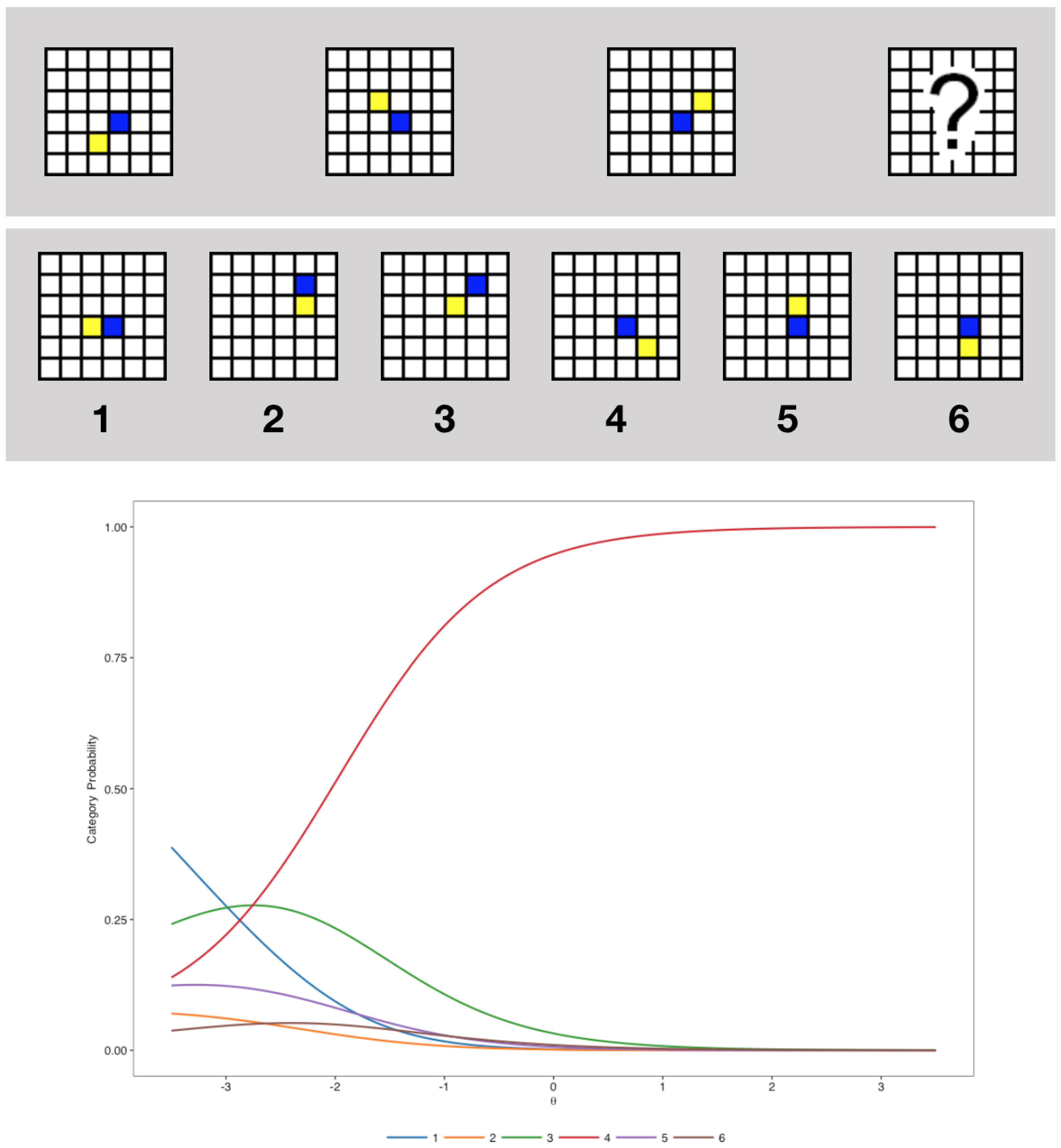
2.2. Instrument
2.3. Binary IRT Modeling
2.3.1. Model Estimation
2.3.2. Model Fit
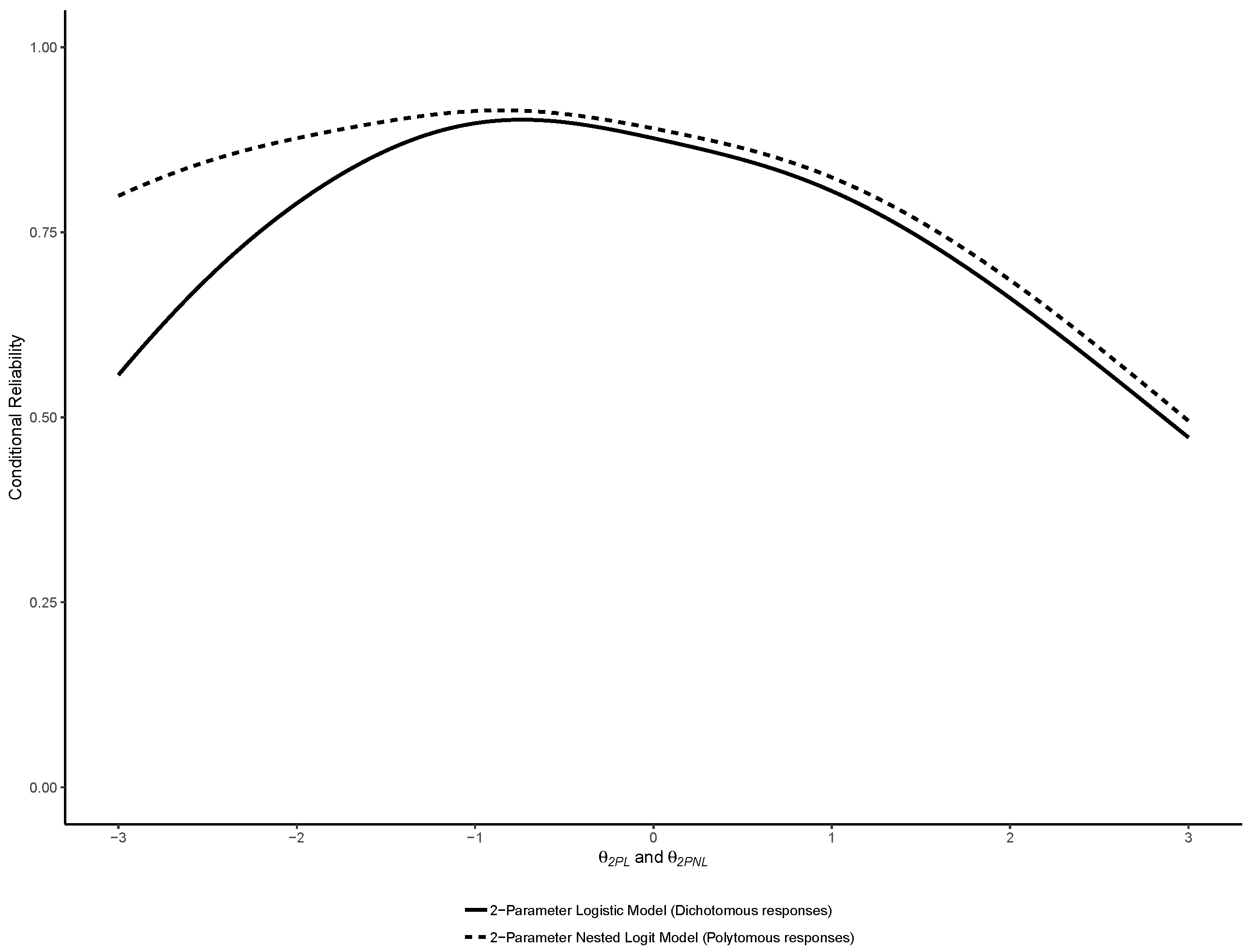
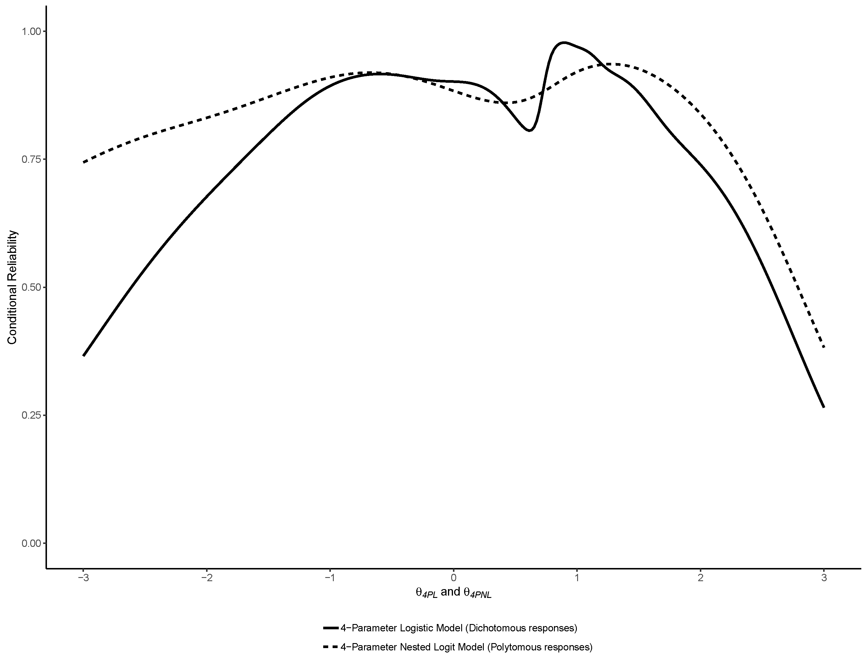
2.3.3. Reliability
2.4. Nominal and Nested Logit IRT Models
2.4.1. Model Estimation
2.4.2. Model Fit
2.4.3. Reliability
3. Results
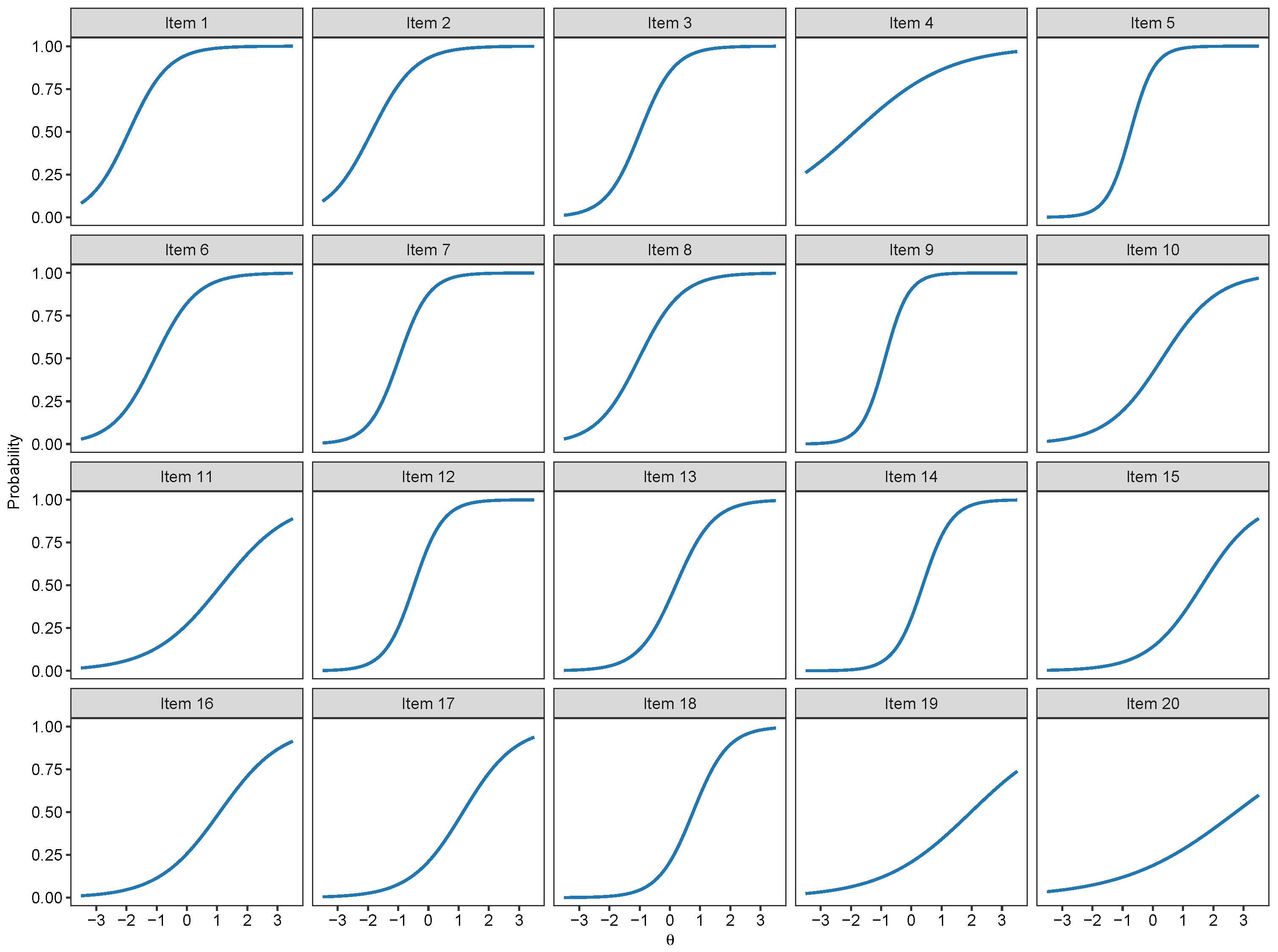
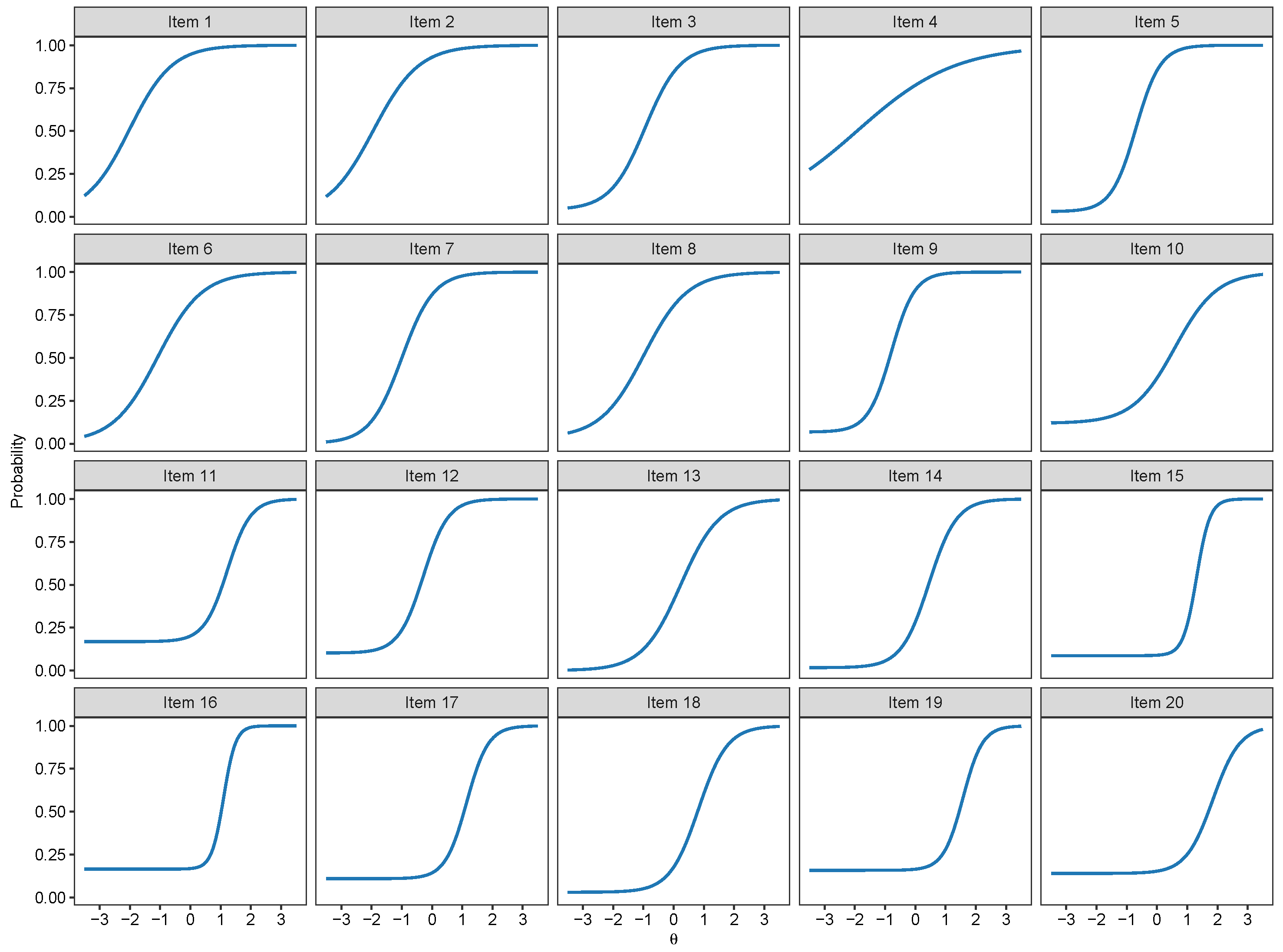
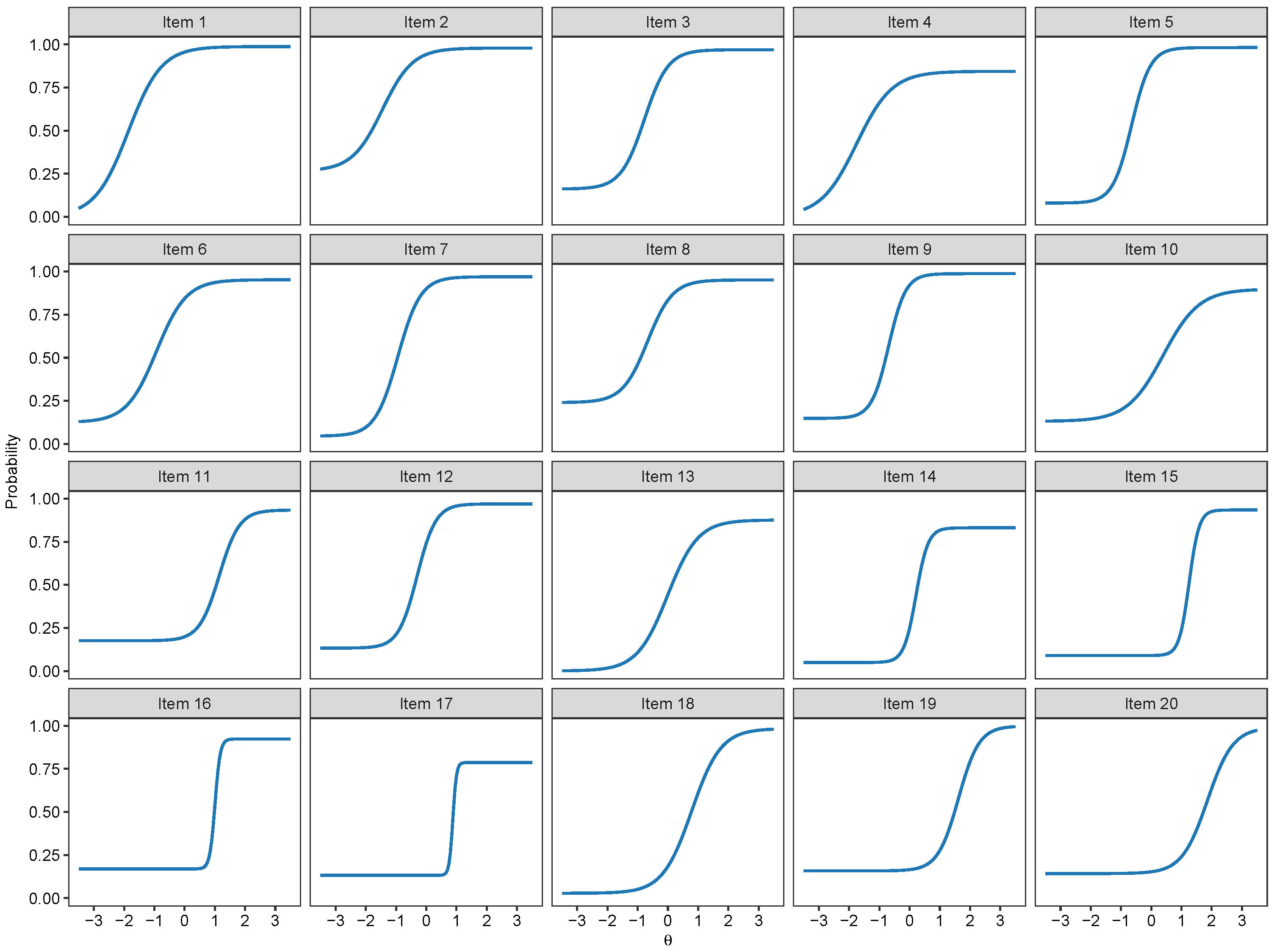
3.1. Binary IRT Models
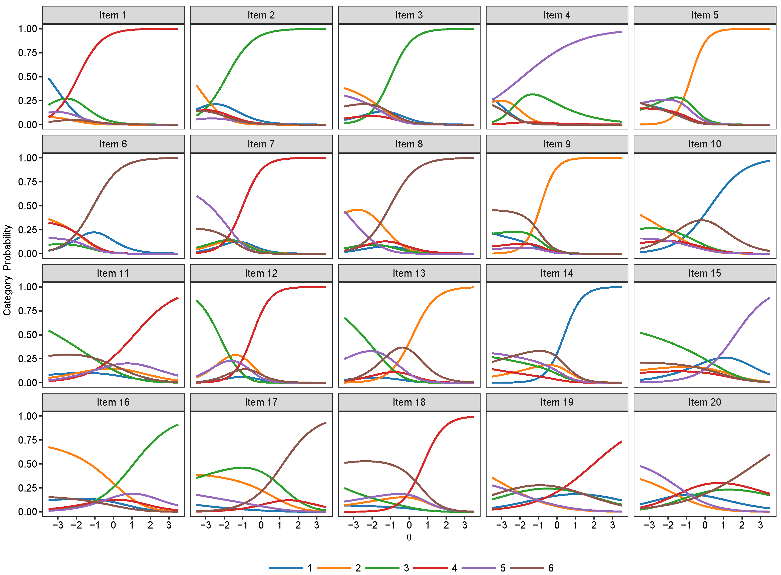
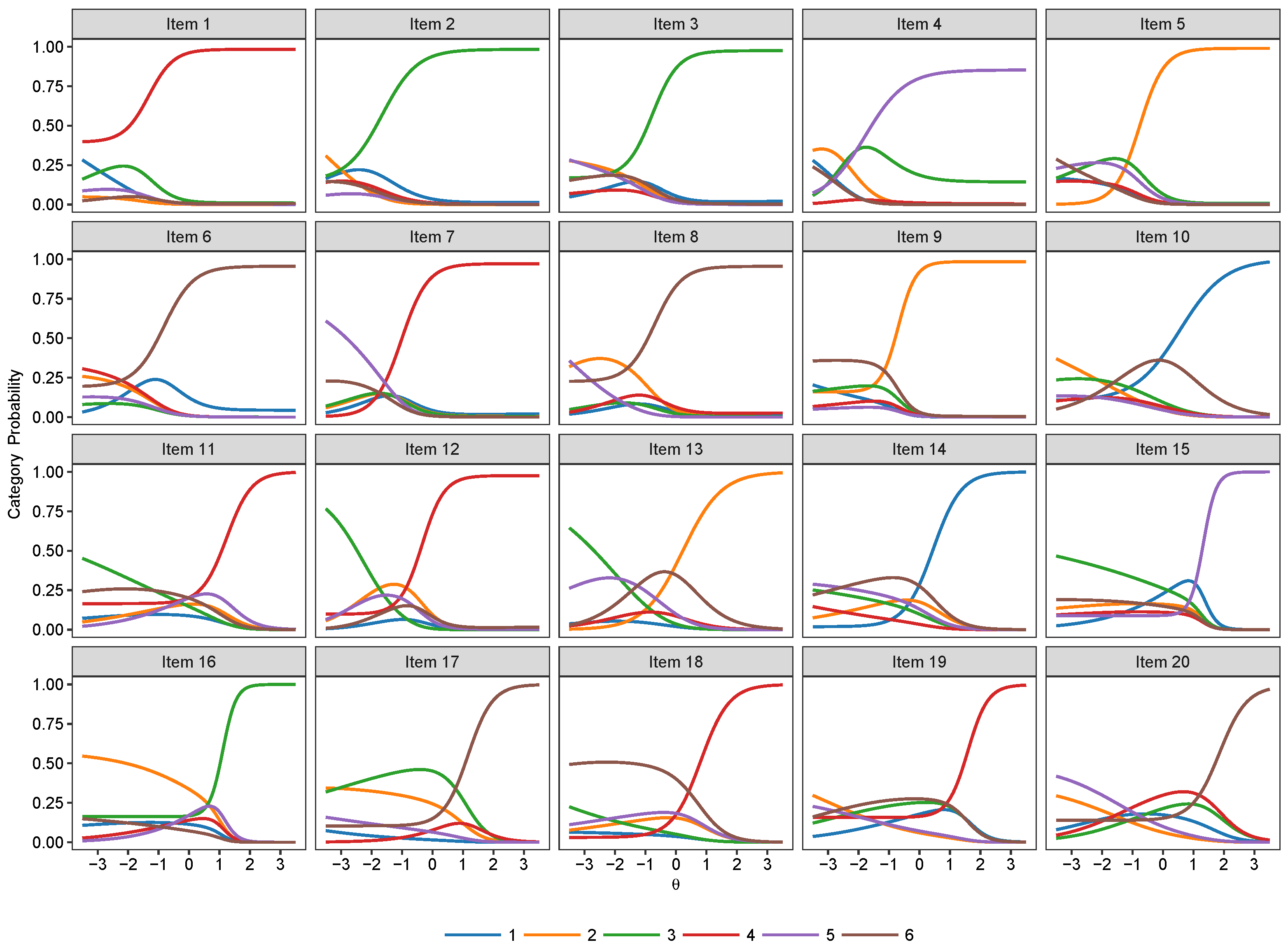
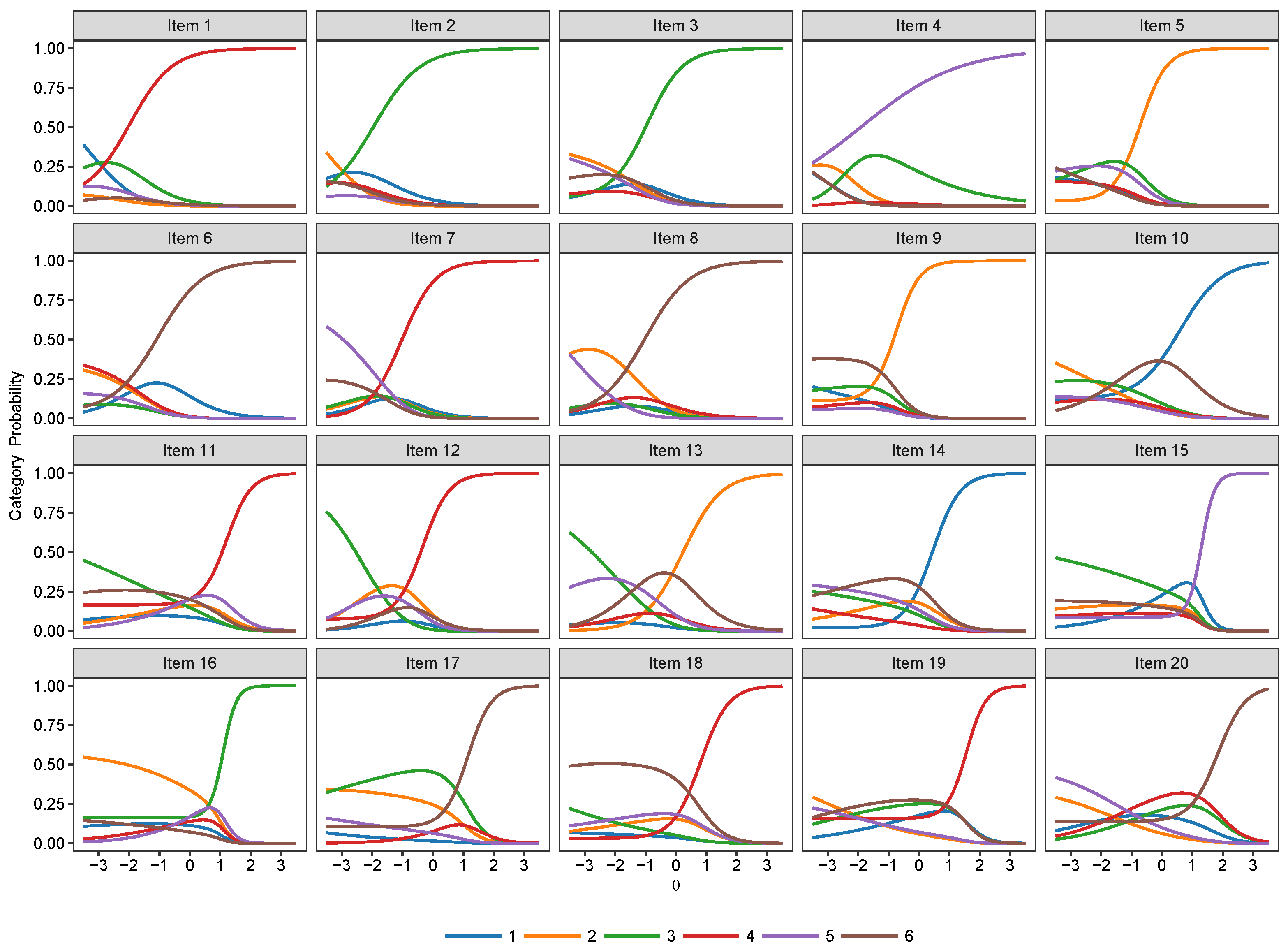
3.2. Nominal Models
4. Discussion
4.1. Theoretical and Practical Implications
4.2. Limitations and Future Research
Author Contributions
Funding
Conflicts of Interest
References
- Bartram, D. Internet recruitment and selection: Kissing frogs to find princes. Int. J. Sel. Assess. 2000, 8, 261–274. [Google Scholar] [CrossRef]
- Laumer, S.; von Stetten, A.; Eckhardt, A. E-assessment. Bus. Inf. Syst. Eng. 2009, 1, 263–265. [Google Scholar] [CrossRef]
- Schmidt, F.L.; Hunter, J. General mental ability in the world of work: Occupational attainment and job performance. J. Personal. Soc. Psychol. 2004, 86, 162. [Google Scholar] [CrossRef] [PubMed]
- Ryan, A.M.; Ployhart, R.E. Applicants’ perceptions of selection procedures and decisions: A critical review and agenda for the future. J. Manag. 2000, 26, 565–606. [Google Scholar] [CrossRef]
- Gilliland, S.W.; Steiner, D.D. Causes and consequences of applicant perceptions of unfairness. In Justice in the Workplace; Cropanzano, R., Ed.; Erlbaum: Hillsdale, NJ, USA, 2001; pp. 175–195. [Google Scholar]
- Tavakol, M.; Dennick, R. Making sense of Cronbach’s alpha. Int. J. Med. Educ. 2011, 2, 53. [Google Scholar] [CrossRef] [PubMed]
- Bock, R.D. Estimating item parameters and latent ability when responses are scored in two or more nominal categories. Psychometrika 1972, 37, 29–51. [Google Scholar] [CrossRef]
- Myszkowski, N.; Storme, M. A snapshot of g? Binary and polytomous item-response theory investigations of the last series of the Standard Progressive Matrices (SPM-LS). Intelligence 2018, 68, 109–116. [Google Scholar] [CrossRef]
- Suh, Y.; Bolt, D.M. Nested logit models for multiple-choice item response data. Psychometrika 2010, 75, 454–473. [Google Scholar] [CrossRef]
- Hüffmeier, J.; Mazei, J.; Schultze, T. Reconceptualizing replication as a sequence of different studies: A replication typology. J. Exp. Soc. Psychol. 2016, 66, 81–92. [Google Scholar] [CrossRef]
- Edelen, M.O.; Reeve, B.B. Applying item response theory (IRT) modeling to questionnaire development, evaluation, and refinement. Qual. Life Res. 2007, 16, 5. [Google Scholar] [CrossRef]
- Kim, S.; Feldt, L.S. The estimation of the IRT reliability coefficient and its lower and upper bounds, with comparisons to CTT reliability statistics. Asia Pac. Educ. Rev. 2010, 11, 179–188. [Google Scholar] [CrossRef]
- Hambleton, R.K.; Van der Linden, W.J. Advances in item response theory and applications: An introduction. Appl. Psychol. Meas. 1982, 6, 373–378. [Google Scholar] [CrossRef]
- Yen, Y.C.; Ho, R.G.; Laio, W.W.; Chen, L.J.; Kuo, C.C. An empirical evaluation of the slip correction in the four parameter logistic models with computerized adaptive testing. Appl. Psychol. Meas. 2012, 36, 75–87. [Google Scholar] [CrossRef]
- Myszkowski, N.; Storme, M. Measuring “good taste” with the visual aesthetic sensitivity test-revised (VAST-R). Personal. Individ. Differ. 2017, 117, 91–100. [Google Scholar] [CrossRef]
- Martín, E.S.; del Pino, G.; Boeck, P.D. IRT Models for Ability-Based Guessing. Appl. Psychol. Meas. 2006, 30, 183–203. [Google Scholar] [CrossRef] [Green Version]
- Matzen, L.B.V.; Van der Molen, M.W.; Dudink, A.C. Error analysis of Raven test performance. Personal. Individ. Differ. 1994, 16, 433–445. [Google Scholar] [CrossRef]
- Raven, J.C. Standardization of progressive matrices, 1938. Br. J. Med. Psychol. 1941, 19, 137–150. [Google Scholar] [CrossRef]
- Beilock, S.L.; Carr, T.H. When high-powered people fail: Working memory and “choking under pressure” in math. Psychol. Sci. 2005, 16, 101–105. [Google Scholar] [CrossRef]
- Gimmig, D.; Huguet, P.; Caverni, J.P.; Cury, F. Choking under pressure and working memory capacity: When performance pressure reduces fluid intelligence. Psychon. Bull. Rev. 2006, 13, 1005–1010. [Google Scholar] [CrossRef] [Green Version]
- Jorgensen, T.D.; Pornprasertmanit, S.; Miller, P.; Schoemann, A.; Rosseel, Y.; Quick, C.; Garnier-Villarreal, M.; Selig, J.; Boulton, A.; Preacher, K.; et al. semTools: Useful Tools for Structural Equation Modeling. Available online: https://cran.r-project.org/web/packages/semTools/semTools.pdf (accessed on 10 July 2019).
- Rosseel, Y. Lavaan: An R Package for Structural Equation Modeling. J. Stat. Softw. 2012, 48. [Google Scholar] [CrossRef]
- Chalmers, R.P. mirt: A multidimensional item response theory package for the R environment. J. Stat. Softw. 2012, 48, 1–29. [Google Scholar] [CrossRef]
- Myszkowski, N.; Storme, M. Judge Response Theory? A Call to Upgrade Our Psychometrical Account of Creativity Judgments. Psychol. Aesthet. Creat. Arts 2019, 13, 167–175. [Google Scholar] [CrossRef]
- Hansen, M.; Cai, L.; Monroe, S.; Li, Z. Limited-Information Goodness-of-Fit Testing of Diagnostic Classification Item Response Theory Models. CRESST Report 840. Natl. Center Res. Eval. Stand. Stud. Test. (CRESST) 2014, 1, 1–47. [Google Scholar]
- Raju, N.S.; Price, L.R.; Oshima, T.; Nering, M.L. Standardized conditional SEM: A case for conditional reliability. Appl. Psychol. Meas. 2007, 31, 169–180. [Google Scholar] [CrossRef]
- Fabrigar, L.R.; Wegener, D.T. Conceptualizing and evaluating the replication of research results. J. Exp. Soc. Psychol. 2016, 66, 68–80. [Google Scholar] [CrossRef]
- Schmidt, S. Shall we really do it again? The powerful concept of replication is neglected in the social sciences. Rev. Gen. Psychol. 2009, 13, 90–100. [Google Scholar] [CrossRef]
- Stroebe, W.; Strack, F. The alleged crisis and the illusion of exact replication. Perspect. Psychol. Sci. 2014, 9, 59–71. [Google Scholar] [CrossRef]
- Suh, Y.; Bolt, D.M. A nested logit approach for investigating distractors as causes of differential item functioning. J. Educ. Meas. 2011, 48, 188–205. [Google Scholar] [CrossRef]
- Bolt, D.M.; Wollack, J.A.; Suh, Y. Application of a multidimensional nested logit model to multiple-choice test items. Psychometrika 2012, 77, 339–357. [Google Scholar] [CrossRef]
- Abbey, B. Instructional and Cognitive Impacts of Web-Based Education; IGI Global: Dauphin County, PA, USA, 1999. [Google Scholar]
- Thissen, D.; Steinberg, L. A response model for multiple choice items. Psychometrika 1984, 49, 501–519. [Google Scholar] [CrossRef]
- Davidshofer, K.; Murphy, C.O. Psychological Testing: Principles and Applications; Pearson/Prentice HallUpper: Saddle River, NJ, USA, 2005. [Google Scholar]
- Duckworth, A.L.; Quinn, P.D.; Lynam, D.R.; Loeber, R.; Stouthamer-Loeber, M. Role of test motivation in intelligence testing. Proc. Natl. Acad. Sci. USA 2011, 108, 7716–7720. [Google Scholar] [CrossRef] [PubMed] [Green Version]


| Model | p | CFI | TLI | RMSEA | AICc | ||
|---|---|---|---|---|---|---|---|
| 1-Parameter Logistic | 2462.597 | 189 | <0.001 | 0.913 | 0.913 | 0.064 | 58,244.74 |
| 2-Parameter Logistic | 1069.812 | 170 | <0.001 | 0.966 | 0.962 | 0.042 | 57,182.90 |
| 3-Parameter Logistic | 251.3807 | 150 | <0.001 | 0.996 | 0.995 | 0.015 | 56,705.29 |
| 4-Parameter Logistic | 196.2342 | 130 | <0.001 | 0.997 | 0.996 | 0.013 | 56,579.87 |
| Item | 1PL Model | 2PL Model | 3PL Model | 4PL Model | ||||||
|---|---|---|---|---|---|---|---|---|---|---|
| logit() | logit() | logit() | ||||||||
| Item 1 | ||||||||||
| Estimate | 2.783 | 1.527 | 2.930 | 1.417 | 2.855 | −4.089 | 1.821 | 3.391 | 0.002 | 0.988 |
| Standard error | 0.072 | 0.105 | 0.113 | 0.104 | 0.157 | 6.671 | ||||
| Item 2 | ||||||||||
| Estimate | 2.569 | 1.391 | 2.605 | 1.326 | 2.575 | −5.002 | 1.999 | 2.898 | 0.266 | 0.979 |
| Standard error | 0.068 | 0.094 | 0.096 | 0.087 | 0.104 | 6.298 | ||||
| Item 3 | ||||||||||
| Estimate | 1.513 | 1.767 | 1.740 | 1.735 | 1.633 | −3.170 | 2.558 | 1.988 | 0.161 | 0.969 |
| Standard error | 0.055 | 0.093 | 0.078 | 0.155 | 0.136 | 2.191 | ||||
| Item 4 | ||||||||||
| Estimate | 1.454 | 0.640 | 1.198 | 0.619 | 1.185 | −5.598 | 1.697 | 2.979 | 0.002 | 0.844 |
| Standard error | 0.055 | 0.054 | 0.048 | 0.051 | 0.057 | 6.083 | ||||
| Item 5 | ||||||||||
| Estimate | 1.291 | 2.543 | 1.878 | 2.462 | 1.719 | −3.465 | 3.222 | 2.097 | 0.080 | 0.982 |
| Standard error | 0.053 | 0.132 | 0.099 | 0.179 | 0.102 | 1.223 | ||||
| Item 6 | ||||||||||
| Estimate | 1.475 | 1.442 | 1.535 | 1.362 | 1.477 | −4.939 | 2.028 | 1.880 | 0.125 | 0.952 |
| Standard error | 0.055 | 0.078 | 0.067 | 0.083 | 0.089 | 6.479 | ||||
| Item 7 | ||||||||||
| Estimate | 1.588 | 2.015 | 1.966 | 1.891 | 1.884 | −6.457 | 2.667 | 2.501 | 0.045 | 0.969 |
| Standard error | 0.056 | 0.106 | 0.089 | 0.097 | 0.084 | 6.179 | ||||
| Item 8 | ||||||||||
| Estimate | 1.404 | 1.412 | 1.448 | 1.389 | 1.365 | −3.355 | 2.415 | 1.622 | 0.240 | 0.951 |
| Standard error | 0.054 | 0.077 | 0.064 | 0.141 | 0.178 | 3.531 | ||||
| Item 9 | ||||||||||
| Estimate | 1.542 | 2.575 | 2.245 | 2.593 | 2.061 | −2.619 | 3.540 | 2.450 | 0.148 | 0.987 |
| Standard error | 0.055 | 0.138 | 0.111 | 0.216 | 0.118 | 0.751 | ||||
| Item 10 | ||||||||||
| Estimate | −0.372 | 1.085 | −0.335 | 1.438 | −0.852 | −2.002 | 1.683 | −0.669 | 0.131 | 0.898 |
| Standard error | 0.050 | 0.059 | 0.046 | 0.149 | 0.172 | 0.285 | ||||
| Item 11 | ||||||||||
| Estimate | −1.137 | 0.878 | −0.991 | 2.603 | −3.188 | −1.597 | 3.013 | −3.462 | 0.176 | 0.934 |
| Standard error | 0.052 | 0.055 | 0.048 | 0.327 | 0.400 | 0.093 | ||||
| Item 12 | ||||||||||
| Estimate | 0.762 | 2.078 | 0.991 | 2.440 | 0.697 | −2.171 | 3.235 | 0.976 | 0.133 | 0.969 |
| Standard error | 0.051 | 0.101 | 0.070 | 0.177 | 0.099 | 0.276 | ||||
| Item 13 | ||||||||||
| Estimate | −0.313 | 1.612 | −0.316 | 1.577 | −0.368 | −7.978 | 1.988 | 0.021 | 0.001 | 0.876 |
| Standard error | 0.049 | 0.079 | 0.054 | 0.076 | 0.055 | 6.064 | ||||
| Item 14 | ||||||||||
| Estimate | −0.662 | 2.121 | −0.802 | 2.191 | −0.992 | −4.072 | 5.037 | −1.078 | 0.049 | 0.831 |
| Standard error | 0.050 | 0.105 | 0.067 | 0.146 | 0.106 | 0.616 | ||||
| Item 15 | ||||||||||
| Estimate | −1.926 | 1.113 | −1.807 | 4.520 | −5.921 | −2.352 | 6.060 | −7.593 | 0.090 | 0.934 |
| Standard error | 0.059 | 0.068 | 0.066 | 0.608 | 0.762 | 0.090 | ||||
| Item 16 | ||||||||||
| Estimate | −1.186 | 0.981 | −1.064 | 5.056 | −5.569 | −1.622 | 11.675 | −11.750 | 0.169 | 0.923 |
| Standard error | 0.053 | 0.058 | 0.051 | 0.754 | 0.841 | 0.071 | ||||
| Item 17 | ||||||||||
| Estimate | −1.399 | 1.153 | −1.321 | 2.815 | −3.228 | −2.099 | 16.917 | −14.883 | 0.132 | 0.787 |
| Standard error | 0.054 | 0.065 | 0.057 | 0.311 | 0.353 | 0.111 | ||||
| Item 18 | ||||||||||
| Estimate | −1.192 | 1.736 | −1.330 | 2.104 | −1.729 | −3.465 | 2.079 | −1.636 | 0.028 | 0.983 |
| Standard error | 0.053 | 0.089 | 0.068 | 0.156 | 0.143 | 0.343 | ||||
| Item 19 | ||||||||||
| Estimate | −1.603 | 0.678 | −1.335 | 3.085 | −4.858 | −1.673 | 2.931 | −4.739 | 0.158 | 0.998 |
| Standard error | 0.056 | 0.054 | 0.050 | 0.520 | 0.759 | 0.077 | ||||
| Item 20 | ||||||||||
| Estimate | −1.808 | 0.532 | −1.463 | 2.248 | −4.156 | −1.817 | 2.369 | −4.404 | 0.143 | 0.990 |
| Standard error | 0.058 | 0.053 | 0.050 | 0.372 | 0.580 | 0.089 | ||||
| Model | p | CFI | TLI | RMSEA | AICc | ||
|---|---|---|---|---|---|---|---|
| Nominal Response | 178.0345 | 90 | <0.001 | 0.972 | 0.941 | 0.018 | 134,347.1 |
| 2-Parameter Nested Logit | 177.3853 | 90 | <0.001 | 0.978 | 0.958 | 0.018 | 133,725.8 |
| 3-Parameter Nested Logit | 126.1003 | 70 | <0.001 | 0.986 | 0.965 | 0.016 | 133,231.1 |
| 4-Parameter Nested Logit | 104.8853 | 50 | <0.001 | 0.986 | 0.952 | 0.019 | 133,195.5 |
| Item | Correct Response | Distractors | ||||||||
|---|---|---|---|---|---|---|---|---|---|---|
| Item 1 | ||||||||||
| Estimate | 1.549 | 2.954 | 0.426 | 1.067 | 0.744 | 1.327 | −0.312 | 2.878 | 1.248 | 1.771 |
| Standard error | 0.103 | 0.113 | 0.535 | 0.341 | 0.383 | 0.382 | 0.805 | 0.523 | 0.579 | 0.554 |
| Item 2 | ||||||||||
| Estimate | 1.397 | 2.614 | −1.189 | −0.297 | −0.123 | −0.442 | −3.219 | −1.154 | −1.509 | −1.669 |
| Standard error | 0.091 | 0.096 | 0.357 | 0.194 | 0.229 | 0.231 | 0.548 | 0.235 | 0.266 | 0.292 |
| Item 3 | ||||||||||
| Estimate | 1.747 | 1.736 | −0.915 | −0.392 | −0.914 | −0.559 | −1.147 | −1.094 | −1.369 | −0.593 |
| Standard error | 0.089 | 0.077 | 0.183 | 0.193 | 0.195 | 0.163 | 0.205 | 0.197 | 0.222 | 0.167 |
| Item 4 | ||||||||||
| Estimate | 0.646 | 1.200 | 0.828 | 2.623 | 2.413 | 0.132 | 2.746 | 6.883 | 4.011 | 0.168 |
| Standard error | 0.053 | 0.048 | 0.650 | 0.646 | 0.671 | 0.821 | 1.150 | 1.122 | 1.136 | 1.476 |
| Item 5 | ||||||||||
| Estimate | 2.417 | 1.819 | 0.648 | 0.180 | 0.386 | −0.077 | 1.893 | 0.351 | 1.343 | −0.259 |
| Standard error | 0.119 | 0.093 | 0.215 | 0.255 | 0.221 | 0.279 | 0.260 | 0.313 | 0.270 | 0.355 |
| Item 6 | ||||||||||
| Estimate | 1.412 | 1.524 | −1.426 | −1.127 | −1.334 | −1.266 | −2.516 | −2.816 | −2.308 | −2.755 |
| Standard error | 0.075 | 0.066 | 0.205 | 0.244 | 0.194 | 0.231 | 0.245 | 0.283 | 0.226 | 0.274 |
| Item 7 | ||||||||||
| Estimate | 1.945 | 1.933 | −0.373 | −0.506 | −1.447 | −1.262 | −0.445 | −0.617 | −1.647 | −1.845 |
| Standard error | 0.098 | 0.085 | 0.171 | 0.179 | 0.218 | 0.237 | 0.171 | 0.184 | 0.267 | 0.291 |
| Item 8 | ||||||||||
| Estimate | 1.425 | 1.457 | −0.868 | −0.485 | −0.010 | −1.611 | 0.098 | −0.573 | 0.507 | −2.450 |
| Standard error | 0.075 | 0.064 | 0.163 | 0.194 | 0.153 | 0.288 | 0.161 | 0.189 | 0.136 | 0.384 |
| Item 9 | ||||||||||
| Estimate | 2.435 | 2.170 | 0.354 | 0.517 | 0.485 | 0.233 | 1.225 | 0.780 | 0.208 | 1.577 |
| Standard error | 0.123 | 0.103 | 0.244 | 0.270 | 0.307 | 0.230 | 0.303 | 0.325 | 0.365 | 0.291 |
| Item 10 | ||||||||||
| Estimate | 1.090 | −0.336 | 0.327 | 0.472 | 0.248 | 1.177 | 0.701 | 0.359 | −0.068 | 2.060 |
| Standard error | 0.058 | 0.046 | 0.131 | 0.144 | 0.155 | 0.123 | 0.137 | 0.145 | 0.161 | 0.122 |
| Item 11 | ||||||||||
| Estimate | 0.875 | −0.991 | 0.318 | −0.397 | 0.567 | −0.116 | 0.613 | 0.501 | 0.834 | 0.817 |
| Standard error | 0.055 | 0.048 | 0.109 | 0.107 | 0.107 | 0.103 | 0.088 | 0.093 | 0.085 | 0.086 |
| Item 12 | ||||||||||
| Estimate | 2.087 | 0.992 | −0.374 | −1.895 | −0.589 | 0.182 | 1.101 | −1.492 | 0.542 | 1.008 |
| Standard error | 0.098 | 0.069 | 0.195 | 0.264 | 0.206 | 0.202 | 0.168 | 0.306 | 0.185 | 0.167 |
| Item 13 | ||||||||||
| Estimate | 1.626 | −0.321 | −0.718 | 0.558 | −0.139 | 0.922 | 0.555 | 1.467 | 1.580 | 2.877 |
| Standard error | 0.078 | 0.055 | 0.216 | 0.211 | 0.201 | 0.196 | 0.226 | 0.197 | 0.197 | 0.185 |
| Item 14 | ||||||||||
| Estimate | 2.096 | −0.804 | −0.577 | −0.696 | −0.539 | −0.221 | −0.613 | −1.659 | −0.334 | 0.435 |
| Standard error | 0.102 | 0.067 | 0.114 | 0.158 | 0.107 | 0.092 | 0.097 | 0.147 | 0.089 | 0.070 |
| Item 15 | ||||||||||
| Estimate | 1.104 | −1.803 | −0.520 | −0.781 | −0.564 | −0.680 | −0.343 | 0.130 | −0.730 | −0.432 |
| Standard error | 0.067 | 0.065 | 0.087 | 0.078 | 0.096 | 0.089 | 0.067 | 0.061 | 0.075 | 0.070 |
| Item 16 | ||||||||||
| Estimate | 0.965 | −1.060 | −0.187 | 0.467 | 0.802 | −0.199 | 1.074 | 0.209 | 0.407 | −0.445 |
| Standard error | 0.057 | 0.050 | 0.092 | 0.113 | 0.112 | 0.125 | 0.076 | 0.086 | 0.084 | 0.106 |
| Item 17 | ||||||||||
| Estimate | 1.118 | −1.309 | 0.310 | 0.512 | 1.364 | 0.149 | 2.761 | 3.379 | 1.632 | 1.423 |
| Standard error | 0.064 | 0.056 | 0.196 | 0.193 | 0.217 | 0.212 | 0.189 | 0.187 | 0.201 | 0.204 |
| Item 18 | ||||||||||
| Estimate | 1.781 | −1.351 | 0.400 | −0.291 | 0.321 | 0.097 | 1.451 | 0.316 | 1.619 | 2.397 |
| Standard error | 0.090 | 0.069 | 0.156 | 0.175 | 0.152 | 0.144 | 0.131 | 0.159 | 0.129 | 0.124 |
| Item 19 | ||||||||||
| Estimate | 0.675 | −1.335 | −0.936 | −0.235 | −0.812 | −0.294 | −1.112 | 0.342 | −0.935 | 0.431 |
| Standard error | 0.053 | 0.050 | 0.110 | 0.074 | 0.104 | 0.073 | 0.103 | 0.061 | 0.094 | 0.060 |
| Item 20 | ||||||||||
| Estimate | 0.533 | −1.463 | −0.720 | 0.390 | 0.318 | −0.680 | −1.051 | 0.208 | 0.541 | −0.578 |
| Standard error | 0.053 | 0.050 | 0.110 | 0.079 | 0.074 | 0.095 | 0.103 | 0.064 | 0.060 | 0.087 |
| Item | Correct Response | Distractors | |||||||||
|---|---|---|---|---|---|---|---|---|---|---|---|
| logit() | |||||||||||
| Item 1 | |||||||||||
| Estimate | 1.443 | 2.843 | −3.065 | 0.396 | 0.927 | 0.668 | 1.132 | −0.323 | 2.768 | 1.196 | 1.623 |
| Standard error | 0.125 | 0.231 | 4.501 | 0.474 | 0.304 | 0.342 | 0.343 | 0.761 | 0.500 | 0.552 | 0.532 |
| Item 2 | |||||||||||
| Estimate | 1.319 | 2.564 | −4.277 | −1.109 | −0.271 | −0.132 | −0.452 | −3.220 | −1.141 | −1.522 | −1.709 |
| Standard error | 0.086 | 0.111 | 4.167 | 0.323 | 0.174 | 0.207 | 0.209 | 0.540 | 0.226 | 0.259 | 0.288 |
| Item 3 | |||||||||||
| Estimate | 1.719 | 1.608 | −2.921 | −0.824 | −0.424 | −0.883 | −0.496 | −1.086 | −1.130 | −1.378 | −0.549 |
| Standard error | 0.149 | 0.131 | 1.645 | 0.164 | 0.176 | 0.177 | 0.146 | 0.194 | 0.193 | 0.216 | 0.158 |
| Item 4 | |||||||||||
| Estimate | 0.625 | 1.181 | −4.813 | 0.684 | 2.387 | 2.171 | −0.076 | 2.602 | 6.763 | 3.888 | −0.230 |
| Standard error | 0.051 | 0.065 | 4.023 | 0.588 | 0.581 | 0.606 | 0.769 | 1.136 | 1.100 | 1.115 | 1.535 |
| Item 5 | |||||||||||
| Estimate | 2.340 | 1.664 | −3.412 | 0.536 | 0.127 | 0.300 | −0.207 | 1.795 | 0.298 | 1.263 | −0.421 |
| Standard error | 0.168 | 0.098 | 1.215 | 0.191 | 0.227 | 0.197 | 0.252 | 0.242 | 0.293 | 0.252 | 0.343 |
| Item 6 | |||||||||||
| Estimate | 1.363 | 1.418 | −3.134 | −1.265 | −0.982 | −1.262 | −1.159 | −2.399 | −2.706 | −2.295 | −2.695 |
| Standard error | 0.125 | 0.158 | 2.550 | 0.183 | 0.217 | 0.176 | 0.208 | 0.230 | 0.264 | 0.220 | 0.263 |
| Item 7 | |||||||||||
| Estimate | 1.826 | 1.854 | −6.090 | −0.338 | −0.431 | −1.327 | −1.119 | −0.425 | −0.565 | −1.599 | −1.751 |
| Standard error | 0.090 | 0.081 | 4.208 | 0.155 | 0.160 | 0.197 | 0.213 | 0.165 | 0.174 | 0.259 | 0.278 |
| Item 8 | |||||||||||
| Estimate | 1.378 | 1.394 | −4.012 | −0.752 | −0.427 | −0.002 | −1.495 | 0.168 | −0.543 | 0.512 | −2.442 |
| Standard error | 0.103 | 0.123 | 4.313 | 0.147 | 0.176 | 0.141 | 0.263 | 0.154 | 0.183 | 0.133 | 0.381 |
| Item 9 | |||||||||||
| Estimate | 2.648 | 1.969 | −2.061 | 0.408 | 0.533 | 0.422 | 0.297 | 1.305 | 0.828 | 0.176 | 1.664 |
| Standard error | 0.200 | 0.116 | 0.370 | 0.225 | 0.249 | 0.285 | 0.212 | 0.298 | 0.320 | 0.364 | 0.286 |
| Item 10 | |||||||||||
| Estimate | 1.461 | −0.870 | −1.983 | 0.317 | 0.456 | 0.250 | 1.137 | 0.701 | 0.356 | −0.061 | 2.034 |
| Standard error | 0.152 | 0.172 | 0.274 | 0.119 | 0.132 | 0.141 | 0.113 | 0.133 | 0.141 | 0.156 | 0.118 |
| Item 11 | |||||||||||
| Estimate | 2.527 | −3.084 | −1.619 | 0.279 | −0.374 | 0.581 | −0.113 | 0.605 | 0.515 | 0.824 | 0.819 |
| Standard error | 0.315 | 0.385 | 0.096 | 0.106 | 0.102 | 0.106 | 0.099 | 0.087 | 0.092 | 0.085 | 0.085 |
| Item 12 | |||||||||||
| Estimate | 2.308 | 0.758 | −2.504 | −0.344 | −1.748 | −0.542 | 0.148 | 1.120 | −1.412 | 0.573 | 0.990 |
| Standard error | 0.159 | 0.093 | 0.359 | 0.180 | 0.243 | 0.191 | 0.188 | 0.162 | 0.296 | 0.178 | 0.161 |
| Item 13 | |||||||||||
| Estimate | 1.593 | −0.374 | −7.481 | −0.630 | 0.525 | −0.116 | 0.852 | 0.615 | 1.446 | 1.596 | 2.837 |
| Standard error | 0.075 | 0.055 | 3.982 | 0.194 | 0.191 | 0.181 | 0.177 | 0.216 | 0.189 | 0.189 | 0.177 |
| Item 14 | |||||||||||
| Estimate | 2.249 | −1.038 | −3.833 | −0.510 | −0.646 | −0.473 | −0.183 | −0.576 | −1.635 | −0.297 | 0.452 |
| Standard error | 0.142 | 0.102 | 0.434 | 0.104 | 0.144 | 0.098 | 0.085 | 0.094 | 0.143 | 0.086 | 0.069 |
| Item 15 | |||||||||||
| Estimate | 4.703 | −6.146 | −2.335 | −0.596 | −0.800 | −0.590 | −0.707 | −0.344 | 0.144 | −0.721 | −0.422 |
| Standard error | 0.663 | 0.831 | 0.089 | 0.088 | 0.079 | 0.097 | 0.089 | 0.067 | 0.061 | 0.075 | 0.070 |
| Item 16 | |||||||||||
| Estimate | 4.626 | −5.091 | −1.638 | −0.152 | 0.446 | 0.824 | −0.214 | 1.089 | 0.205 | 0.404 | −0.452 |
| Standard error | 0.608 | 0.675 | 0.072 | 0.088 | 0.112 | 0.115 | 0.118 | 0.075 | 0.086 | 0.084 | 0.105 |
| Item 17 | |||||||||||
| Estimate | 2.613 | −3.013 | −2.142 | 0.328 | 0.520 | 1.452 | 0.162 | 2.774 | 3.387 | 1.618 | 1.434 |
| Standard error | 0.277 | 0.313 | 0.117 | 0.182 | 0.180 | 0.211 | 0.198 | 0.188 | 0.186 | 0.201 | 0.202 |
| Item 18 | |||||||||||
| Estimate | 2.210 | −1.798 | −3.415 | 0.377 | −0.242 | 0.321 | 0.122 | 1.444 | 0.342 | 1.618 | 2.407 |
| Standard error | 0.159 | 0.143 | 0.300 | 0.144 | 0.160 | 0.141 | 0.133 | 0.129 | 0.156 | 0.127 | 0.122 |
| Item 19 | |||||||||||
| Estimate | 3.167 | −4.950 | −1.672 | −0.901 | −0.241 | −0.773 | −0.300 | −1.090 | 0.344 | −0.911 | 0.434 |
| Standard error | 0.523 | 0.760 | 0.076 | 0.104 | 0.076 | 0.100 | 0.074 | 0.101 | 0.061 | 0.092 | 0.060 |
| Item 20 | |||||||||||
| Estimate | 2.233 | −4.111 | −1.827 | −0.659 | 0.381 | 0.315 | −0.628 | −1.018 | 0.205 | 0.537 | −0.551 |
| Standard error | 0.357 | 0.552 | 0.089 | 0.102 | 0.079 | 0.073 | 0.089 | 0.100 | 0.064 | 0.060 | 0.084 |
| Item | Correct Response | Distractors | ||||||||||
|---|---|---|---|---|---|---|---|---|---|---|---|---|
| logit() | logit() | |||||||||||
| Item 1 | ||||||||||||
| Estimate | 2.447 | 3.234 | 0.395 | 0.983 | 0.413 | 0.955 | 0.677 | 1.174 | −0.314 | 2.778 | 1.189 | 1.640 |
| Item 2 | ||||||||||||
| Estimate | 1.733 | 2.875 | 0.149 | 0.983 | −1.077 | −0.283 | −0.142 | −0.448 | −3.143 | −1.150 | −1.530 | −1.697 |
| Item 3 | ||||||||||||
| Estimate | 2.364 | 1.832 | 0.168 | 0.975 | −0.801 | −0.428 | −0.904 | −0.482 | −1.052 | −1.132 | −1.392 | −0.534 |
| Item 4 | ||||||||||||
| Estimate | 1.517 | 2.702 | 0.016 | 0.852 | 0.690 | 2.391 | 2.175 | 0.049 | 2.619 | 6.790 | 3.913 | 0.015 |
| Item 5 | ||||||||||||
| Estimate | 2.474 | 1.897 | 0.001 | 0.990 | 0.500 | 0.121 | 0.258 | −0.309 | 1.749 | 0.288 | 1.212 | −0.542 |
| Item 6 | ||||||||||||
| Estimate | 2.063 | 1.698 | 0.192 | 0.956 | −1.277 | −1.048 | −1.307 | −1.155 | −2.392 | −2.766 | −2.329 | −2.673 |
| Item 7 | ||||||||||||
| Estimate | 2.323 | 2.377 | 0.002 | 0.972 | −0.336 | −0.421 | −1.341 | −1.087 | −0.424 | −0.556 | −1.613 | −1.706 |
| Item 8 | ||||||||||||
| Estimate | 2.260 | 1.575 | 0.225 | 0.955 | −0.765 | −0.426 | 0.005 | −1.551 | 0.166 | −0.539 | 0.515 | −2.474 |
| Item 9 | ||||||||||||
| Estimate | 3.508 | 2.443 | 0.159 | 0.985 | 0.447 | 0.560 | 0.460 | 0.325 | 1.343 | 0.851 | 0.212 | 1.691 |
| Item 10 | ||||||||||||
| Estimate | 1.357 | −0.757 | 0.104 | 0.999 | 0.332 | 0.473 | 0.278 | 1.152 | 0.711 | 0.368 | −0.041 | 2.048 |
| Item 11 | ||||||||||||
| Estimate | 2.444 | −3.023 | 0.165 | 1.000 | 0.286 | −0.378 | 0.583 | −0.110 | 0.608 | 0.512 | 0.829 | 0.820 |
| Item 12 | ||||||||||||
| Estimate | 2.766 | 0.948 | 0.098 | 0.976 | −0.327 | −1.817 | −0.519 | 0.160 | 1.131 | −1.481 | 0.590 | 0.997 |
| Item 13 | ||||||||||||
| Estimate | 1.576 | −0.356 | 0.000 | 1.000 | −0.640 | 0.555 | −0.096 | 0.890 | 0.607 | 1.466 | 1.611 | 2.861 |
| Item 14 | ||||||||||||
| Estimate | 2.176 | −0.980 | 0.019 | 1.000 | −0.510 | −0.661 | −0.469 | −0.177 | −0.579 | −1.646 | −0.297 | 0.453 |
| Item 15 | ||||||||||||
| Estimate | 4.743 | −6.281 | 0.088 | 1.000 | −0.585 | −0.799 | −0.588 | −0.704 | −0.348 | 0.136 | −0.727 | −0.428 |
| Item 16 | ||||||||||||
| Estimate | 4.613 | −5.115 | 0.162 | 1.000 | −0.155 | 0.454 | 0.830 | −0.225 | 1.087 | 0.210 | 0.413 | −0.458 |
| Item 17 | ||||||||||||
| Estimate | 2.496 | −2.914 | 0.104 | 1.000 | 0.357 | 0.555 | 1.501 | 0.196 | 2.792 | 3.409 | 1.641 | 1.454 |
| Item 18 | ||||||||||||
| Estimate | 2.146 | −1.745 | 0.031 | 1.000 | 0.359 | −0.264 | 0.303 | 0.102 | 1.437 | 0.332 | 1.611 | 2.398 |
| Item 19 | ||||||||||||
| Estimate | 3.048 | −4.844 | 0.157 | 0.998 | −0.912 | −0.245 | −0.784 | −0.300 | −1.096 | 0.343 | −0.917 | 0.433 |
| Item 20 | ||||||||||||
| Estimate | 2.217 | −4.113 | 0.139 | 0.991 | −0.666 | 0.393 | 0.319 | −0.633 | −1.023 | 0.206 | 0.540 | −0.555 |
© 2019 by the authors. Licensee MDPI, Basel, Switzerland. This article is an open access article distributed under the terms and conditions of the Creative Commons Attribution (CC BY) license (http://creativecommons.org/licenses/by/4.0/).
Share and Cite
Storme, M.; Myszkowski, N.; Baron, S.; Bernard, D. Same Test, Better Scores: Boosting the Reliability of Short Online Intelligence Recruitment Tests with Nested Logit Item Response Theory Models. J. Intell. 2019, 7, 17. https://0-doi-org.brum.beds.ac.uk/10.3390/jintelligence7030017
Storme M, Myszkowski N, Baron S, Bernard D. Same Test, Better Scores: Boosting the Reliability of Short Online Intelligence Recruitment Tests with Nested Logit Item Response Theory Models. Journal of Intelligence. 2019; 7(3):17. https://0-doi-org.brum.beds.ac.uk/10.3390/jintelligence7030017
Chicago/Turabian StyleStorme, Martin, Nils Myszkowski, Simon Baron, and David Bernard. 2019. "Same Test, Better Scores: Boosting the Reliability of Short Online Intelligence Recruitment Tests with Nested Logit Item Response Theory Models" Journal of Intelligence 7, no. 3: 17. https://0-doi-org.brum.beds.ac.uk/10.3390/jintelligence7030017