1. Introduction
Analysis of human gaits has long been an active area of research, and many systems have been proposed for observing and differentiating different gait patterns and their irregularities in the literature. Many of these existing systems use appearance-based approaches by extracting features and/or positions from the images captured from different video sequences using high-speed video cameras with frame rates of 50–200 Hz. Many studies have reported that image feature extraction using biomechanical models can allow quantitative analysis of specific gait characteristics, such as joint moments and powers (i.e., kinetic analysis), joint angles, angular velocities and angular accelerations (i.e., kinematic analysis) [
1]. The testing protocol of these systems includes placing the optical markers near anatomical landmarks of the body and features related to various gait patterns are extracted from video sequences. Parametric models have been used extensively to describe a set of successive image observations. A vision-based three-dimensional (3D) modeling of motions of a human subject can be achieved by using volumetric bodies (e.g., using cylinders) that represent the flesh of the human subject and a simple collection of segments with joint angles representing the skeletal structure of the human body [
2]. Alternatively, 2D models that represent the projection of 3D data onto an imaging plane can also be used (i.e., 2D/3D contour modeling [
3]). However, since different kinetic and kinematic methods have been developed from these sophisticated and expensive visual gait analysis systems, it can be rather challenging to directly compare the gait analysis results from different systems/methods, as there is no standardization in the visual gait analysis methodology.
In addition, the variables that can be measured during gait analysis depend on the technique and sensors selected, which makes the direct comparison of gait analysis results derived from different gait sensing systems even much more difficult. The most commonly-reported gait measurement data include the temporospatial parameters, which include walking speed, body rotations, step time, step length and the durations of the stance phase and the swing phase [
4]. A basic inertial measurement unit (IMU) that includes 3D gyroscopes and accelerometers can measure angular velocity and linear acceleration for each of the X/Y/Z axes, respectively, and these inexpensive IMUs have been used as wearable sensors that provide a powerful option for human gait analysis [
4,
5,
6]. For example, Aminian et al. [
4] and Selles et al. [
5] reported methods of measuring both terminal contact (TC) that defines the beginning of the swing phase, as well as the initial contact (IC) that defines the beginning of the gait cycle timing information using those body-worn sensors. On the other hand, Yoshida et al. [
6] used an accelerometer/IMU sensor attached to the patient’s waist and observed frequency peaks in the anterior plane to detect leg injury. Boutaayamou et al. [
7] developed a signal processing algorithm to automatically extract, on a stride-by-stride basis, four consecutive fundamental events of walking, i.e., heel strike (HS), toe strike (TS), heel-off (HO) and toe-off (TO), from wireless accelerometers applied to the right and left foot. This accelerometer-based event identification was validated in seven healthy volunteers and a total of 247 trials against reference data provided by a force plate, a kinematic 3D analysis system and a video camera. An ambulatory monitoring method using an IMU sensor for patients with Parkinson’s disease has also been developed [
8,
9].
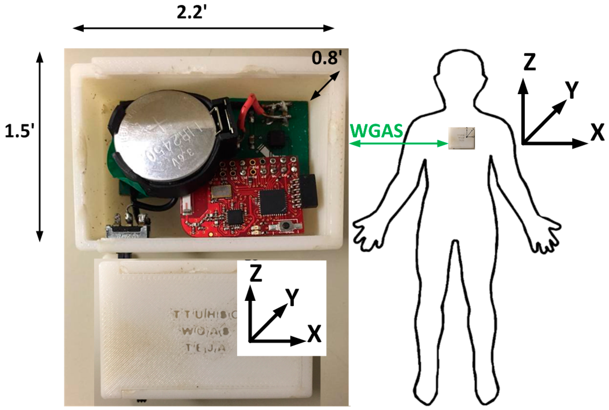
We have, therefore, designed a custom low-cost wireless gait analysis sensor (WGAS), which can be used for both fall detection and gait analysis. We reported to have demonstrated measured fall detection rates of 99% in classification accuracies among young volunteers using a similar WGAS with the BP-ANN and SVM classification algorithms [
10,
11,
12]. This paper, however, studies and reports our new WGAS that is used specifically for gait analysis to detect patients with balance disorders among normal subjects while using various classification algorithms and input features to check the speed and accuracy of each classifier. This WGAS is placed and tested at the T4 position on the back of each subject, as shown in
Figure 1. For the learning of the classification algorithms, we will first use the following six input features for the X/Y/Z axes extracted from the raw data taken from the WGAS (i.e.,
Rω: range of angular velocity;
RA: range of acceleration, as shown in Equations (1) and (2)). They are used as one of the input features sets for these classifiers that yield excellent classification accuracies, and the details of the WGAS and our experimentation and analysis will be explained next.
Wireless Gait Analysis Sensor
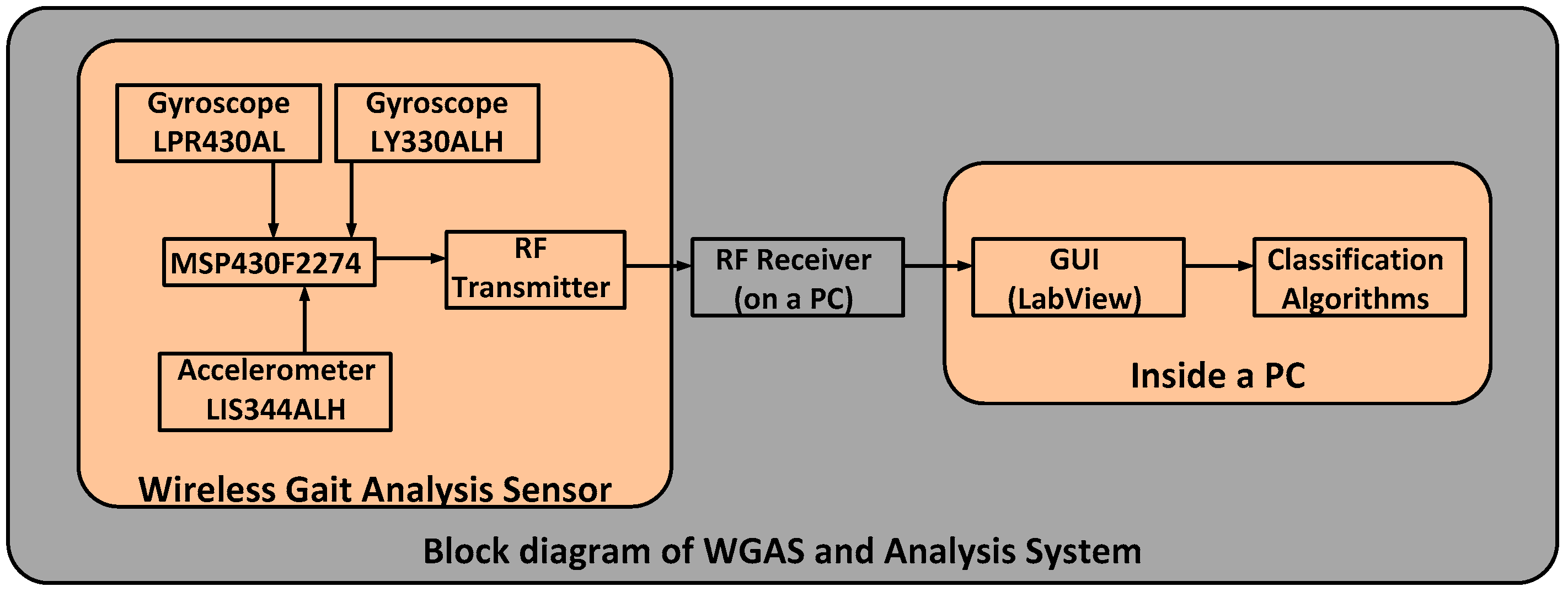
The custom-designed WGAS consists of a three-axis linear accelerometer IC, a single-axis gyroscope IC and a dual-axis gyroscope IC to measure 3D human body translations and rotations during a gait pattern; these ICs are designed with the help of micro-electrical and mechanical system (MEMS) sensors. Our WGAS measures the linear acceleration and angular rotations of the body movements, and there is no need for a magnetometer for our application of gait analysis and gait classification. Furthermore, the sensor has a dual- and single-axis gyroscope instead of a tri-axial gyroscope, because the particular analog MEMS tri-axial gyroscope was not available on the market during the design of the WGAS, but it is now. The future design of our WGAS can have a more compact IMU with a tri-axial single accelerometer IC and a single-gyroscope IC. However, we do not believe this will affect the sensing results whether one IC or two ICs are used. The details of these ICs with their manufacturers’ information can be found in [
10,
11]. This WGAS system is supported by a Texas Instruments (TI) MSP430 microcontroller (Texas Instruments, Dallas, TA, USA) and a wireless 2.4 GHz USB transceiver using the TI SimpliciTI™ protocol (Texas Instruments, Dallas, TA, USA) with a wireless communication range of ~12 meters (40 ft). An overall simplified system block diagram for the WGAS analysis system is shown in
Figure 2.
The two AAA batteries used in our earlier wired sensor [
13] were replaced by a single rechargeable Li-ion coin battery, providing a battery lifetime of ~40 h of continuous operation time with each recharge. The PCB, coin battery and the microcontroller are placed in a specially-designed 3D-printed plastic box (2.2′ × 1.5′ × 0.8′) with a total weight of 42 g. The design of the box was done with the 3D modeling software Rhinoceros (Rhino, Robert McNeel & Associates, WA, USA) and printed using a 3D printer with acrylonitrile butadiene styrene (ABS) plastic. The box has a sliding lid and is shown in
Figure 1. The accelerometer data are sampled at 160 Hz and digitized to eight bits, with its output scaled to ±6 g at Δ V = ±6 g/VDD (VDD, Supply voltage = 3.6 V) for each axis. The gyroscope data are also sampled at 160 Hz and digitized to eight bits, with its output scaled to 300°/s (dps) at ΔV = ±300 dps. Multiplied by So (note the typical So (sensitivity) value is 3.752 mV/dps for the accelerometer and 3.33 mV/dps for the gyroscopes). The sensor orientation and position on the body during testing are also shown in
Figure 1. The sensor is carefully secured to the subjects during testing to avoid artifacts. A cloth is used to secure the WGAS by tying it tightly at the T4 position of the patient’s back. The cloth is also attached to the shirt of the subject by using plastic tape. In addition, Velcro is attached to the sensor box that firmly attaches to the shirt, as well, to make sure that the sensor does not move around during the DGI tests shown in
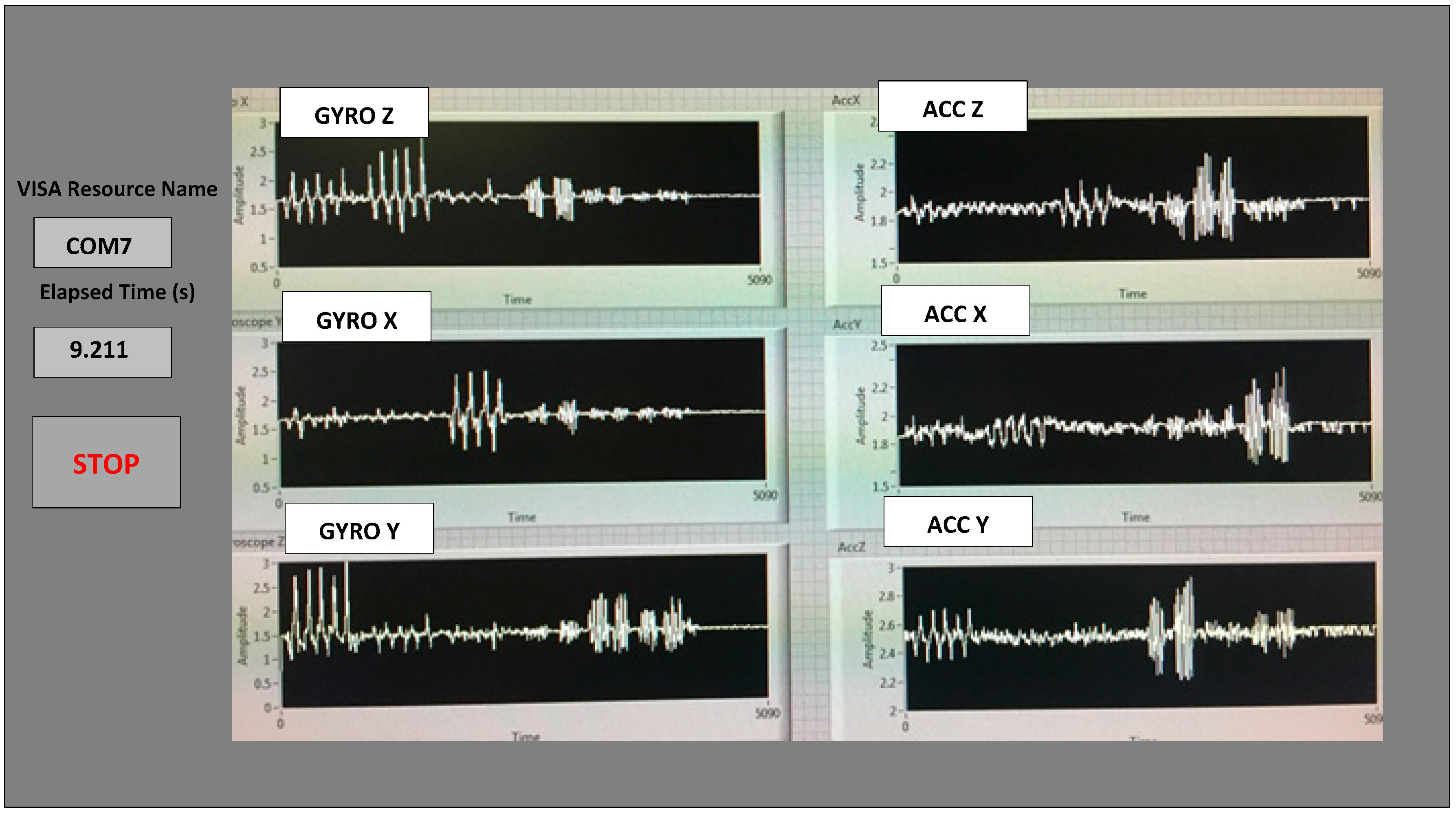
Table 1. The method described above proved that it significantly reduced the outliers in the measured datasets from the sensor. The microcontroller and the transceiver unit enable the real-time wireless transmission of the six-dimensional gait data to the nearby PC, where a LABVIEW™ program is used for designing the graphical user interface (GUI), as shown in
Figure 3. The DC values for the six signals are not the same as the battery charges and discharges, and the calibration to make them the same DC level was not done to simplify the WGAS design, as we have ascertained that the detected AC signals from WGAS are really the ones that contain the most useful gait information, as will be shown in the remaining of this paper.
2. Experimental Section
All four patients and the three normal subjects performed the 7 Dynamic Gait Index (DGI) tests [
10,
14] with the details shown in
Table 1. Therefore, a total of 28 dynamic gait tests were performed on 4 patients and 21 tests on three normal subjects. During all of the tests, the WGAS is placed at the T4 position (at back) for all of the subjects involved. Our WGAS sensor has been accepted by the Texas Tech University Health Sciences Center (TTUHSC) Internal Review Board (IRB) with study title “Fall risk identification and assessment using body worn sensors (CRI12-030 Fall study)”.
The six features of the raw data on range from the gyroscopes and the accelerometers from all of the testing subjects are important, and they form the inputs for training the classification algorithms. These include the range of angular velocity in the X/Y/Z direction (i.e.,
Rωx, from “GYRO X”;
Rωy, from “GYRO Y”; and
Rωz, from “GYRO Z”) and the range of acceleration in the X/Y/Z direction (i.e.,
RAx, from “ACC X”;
RAy, from “ACC Y”; and
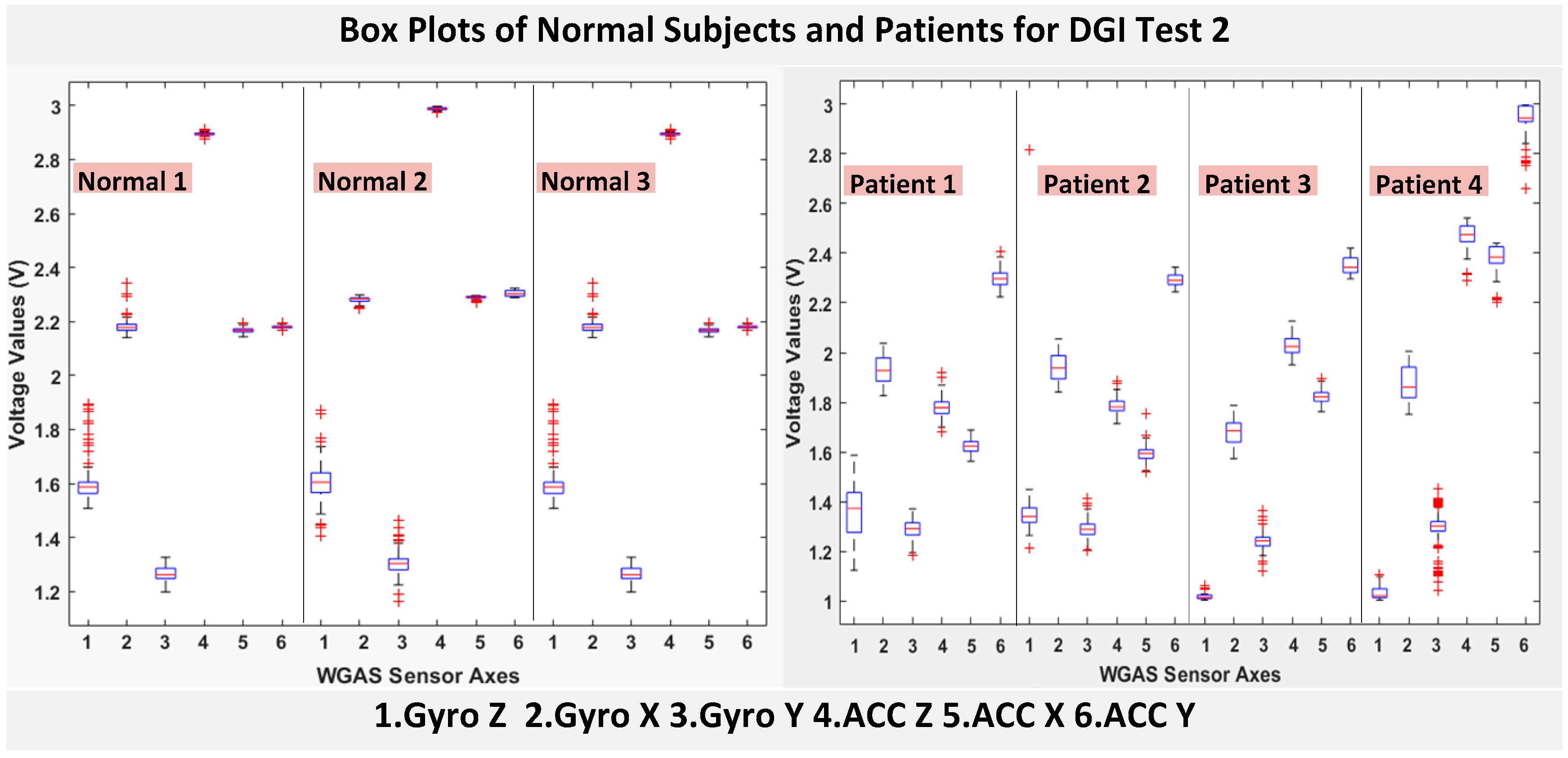
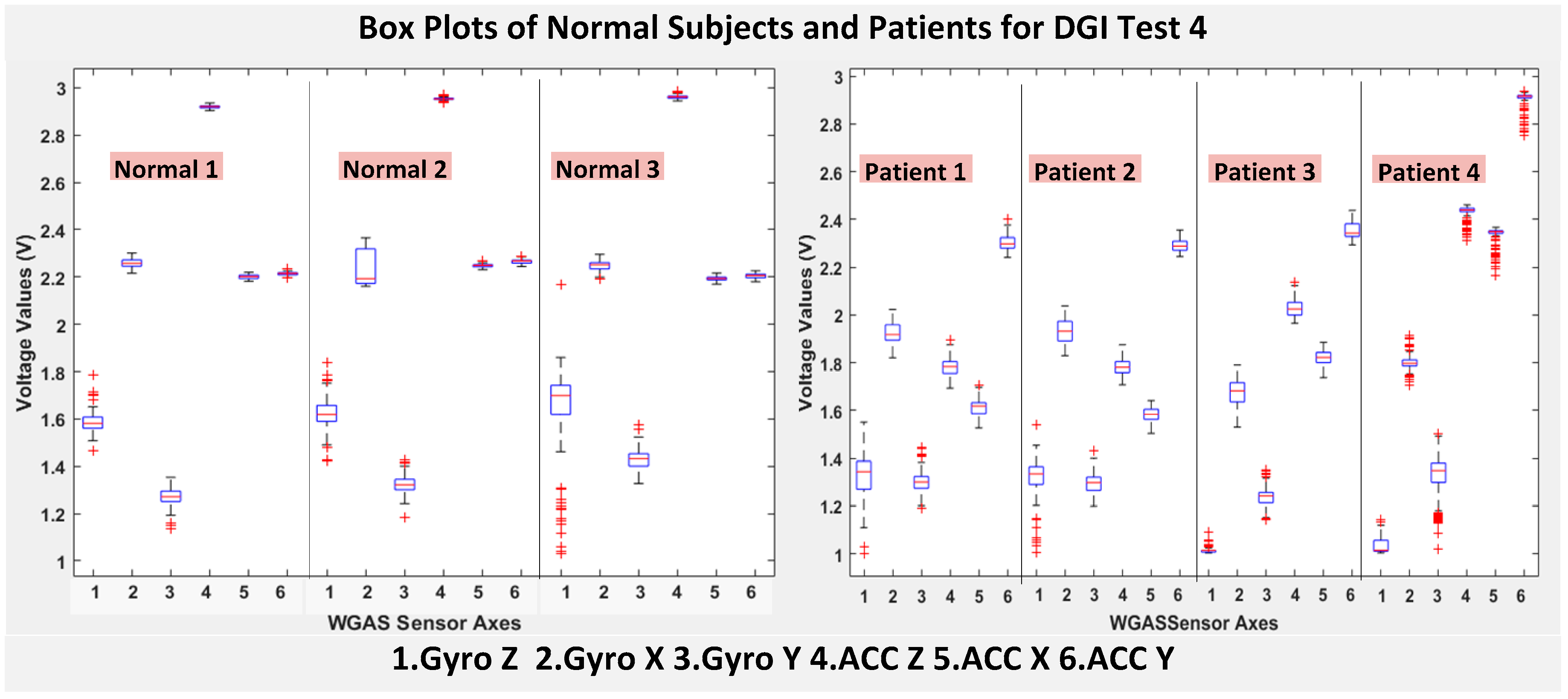
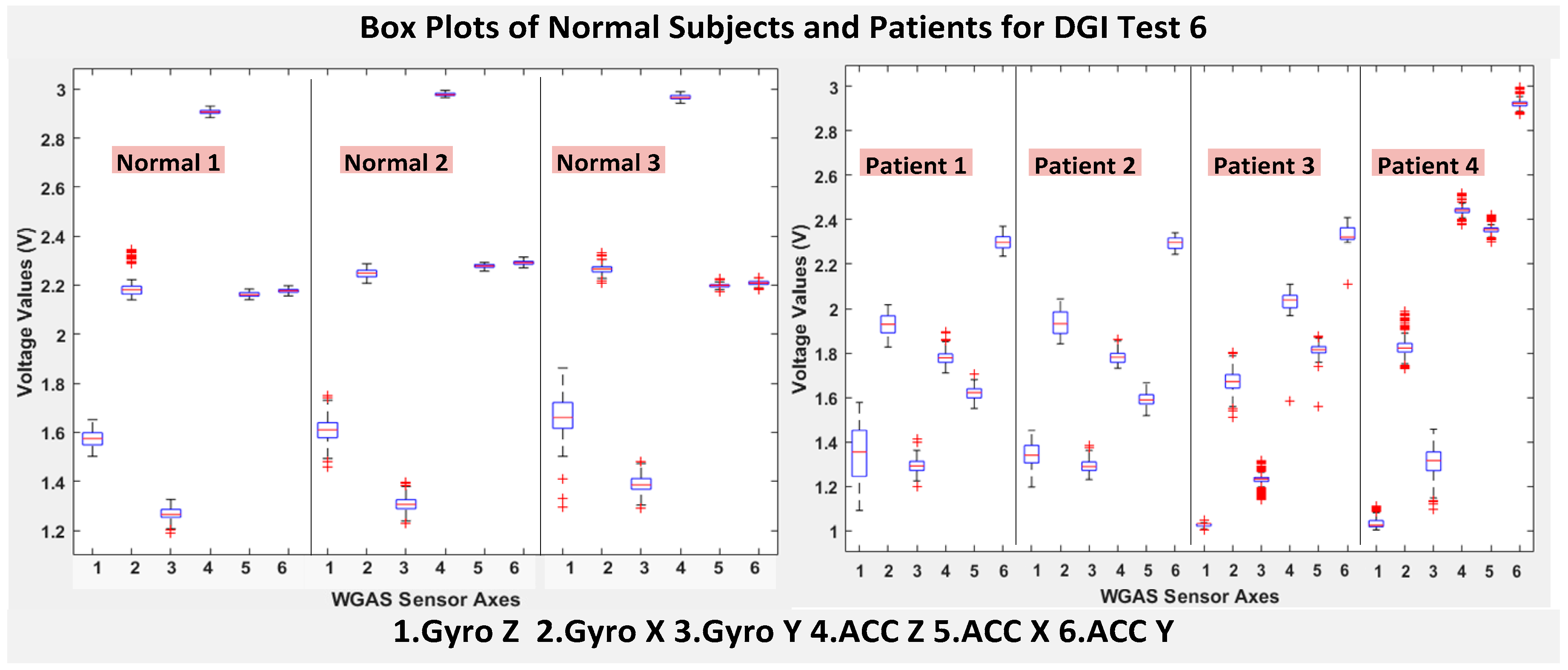
RAz, from “ACC Z”). The data were obtained using a 1.7 GHz PC with 4 GB of RAM, Windows 8 OS, and using MATLAB R2015b. We compared the box plots of the four patients and three normal subjects to show several key test data statistics: the median, mean, range (highest to lowest values) and interquartile range (IQR) of DGI Tests 2, 3, 4 and 6, as shown in
Figure 4,
Figure 5,
Figure 6 and
Figure 7. These four DGI tests are selected and plotted here; they can show better visual comparisons than the other three DGI tests; some detailed statistics of all DGI tests are also listed later in this paper i.e., at the end of
Section 2 (e.g.,
Figure 8 and
Figure 9, etc.)
Moreover, the average of STDEV (i.e., standard deviation), Range, Mean, Median, and IQR of DGI Tests 2 and 7 are calculated and shown in
Table 2 and
Table 3.
As shown in
Figure 4, the box plots of the patients’ data appear to be mostly larger than those of the normal subjects for DGI Test 2 for all extracted features, and they look significantly tighter for all of the 3-axial acceleration data for all DGI tests as shown in
Figure 4,
Figure 5,
Figure 6 and
Figure 7 (i.e., “ACC X”, “ACC Y” and “ACC Z”). The tighter the box plot distributions suggest the normal subjects are walking more steadily with less wobbling or sways than patients during the DGI tests.
Besides the larger box plots associated with larger STDEV and IQR for patients, in all box plots, we have also observed the median/mean values of the acceleration measured on the X and Z axes (i.e., “ACC X”, “ACC Z”) of the normal subjects are significantly larger from those of patients for all of the DGI tests, and we have shown this difference in
Table 2 and
Table 3 for DGI Test 2 and Test 7 as examples for better illustration. This contrast might be explained because walking gaits of normal subjects are considerably different from those of patients, where they walk freely with more accelerations along the X/Z direction from their center of mass (CoM), while patients of balance disorders typically walk with a decrease of speed, shortened stride length and other associated factors [
4,
5]. It is also interesting to notice that the median/mean values of ACC Y of the normal subjects are not so different from those of patients. This might be due to that during the DGI tests, the Y axis is parallel to the walking direction, while the X and Z axes are perpendicular to the walking direction, and therefore, we did not see much change in the median/mean values along the Y axis. We will need to look at these effects related to the median/mean values from accelerometers closely after more patient data can be collected to hopefully understand them better.
Moreover, as mentioned before, when the gait data’s STDEV is smaller, one would expect the walking to be more steady or stable. We can indeed see in the box plots and tables that the normal subjects’ STDEV values on Gyro X and Y and ACC X, Y and Z are all smaller than those of patients. However, the normal subjects’ STDEV data of Gyro Z are actually than that of the patients, suggesting that normal subjects may rotate their bodies around the Z axis naturally more and with more variation than patients of balance disorders; their faster walking speed than the patients may contribute to this effect, as well. Note we would really need to collect more patient gait data to improve the statistics and analysis details especially on the gyroscope data, as we can see that for all seven DGI tests, the STDEVs of Gyro Z data for Patients No. 1 and No. 2 are so different from those of Patients No. 3 and No. 4 (see
Figure 4,
Figure 5,
Figure 6 and
Figure 7). To see this better, we have also shown the values of the STDEV for normal subjects and patients for DGI Test 2 in
Table 4. Therefore, one can see from
Table 4 that the STDEVs of Gyro Z for normal subjects are actually slightly lower than those of “Patient 1” and “Patient 2”, but much greater than those of “patient “and “Patient 4”; therefore, the average STDEV of Gyro Z among normal subjects becomes larger than that of patients.
Finally, not surprisingly,
Table 3 shows that the average range values of Gyro X, Y, Z and also ACC X, Y, Z for the patients’ gait data are all greater than those of the normal subjects’ for all of the DGI tests, except for the range of the Gyro Z data of the DGI Test 7, probably for the reasons stated before that the normal subjects may rotate their bodies around the Z axis naturally more with faster walking speeds and, therefore, with more variation and range difference than patients of balance disorders. Moreover,
Figure 4,
Figure 5,
Figure 6 and
Figure 7 show the box plots of DGI Tests 2, 3, 4 and 6 that group normal subjects as one group vs. patients as another group. From these points, the DGI Tests 2, 3, 4 and 6 present as better tests than the DGI Tests 1, 5 and 7 for differentiating patients from normal subjects. Having checked those basic data statistics, we have decided to first use the range values of the patients and normal subjects from all six sensor axes and for all 7 DGI tests taken as the single input features for the classification algorithms. We will later also use STDEV, etc., as input features to these classifiers and compare them, as well.
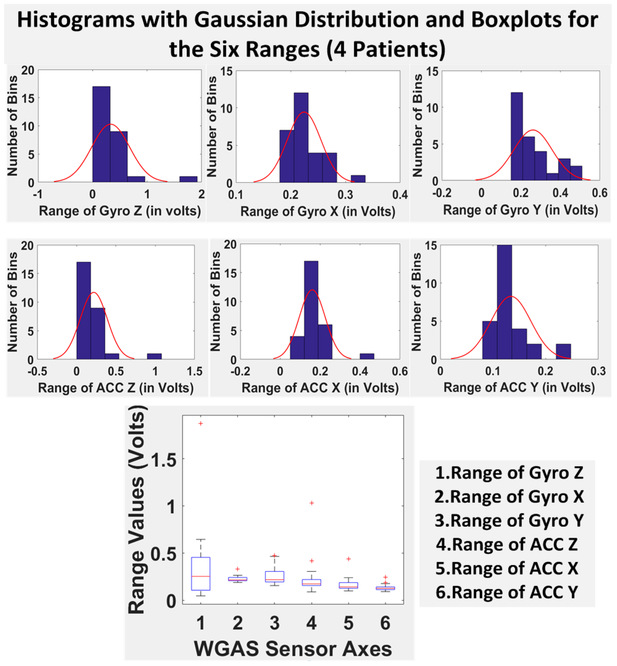
Finally, we have shown in
Table 5 the STDEV, range, median, mean and IQR for normal subjects vs. patients for all seven DGI tests. To see the distributions on range better, the histograms of the data with normal distribution are now also shown for each of the six features for both patients and normal subjects in
Figure 8 and
Figure 9. The box plots of normal subjects and patients are also shown for these six features. It can be clearly seen that the features related to the acceleration data (i.e., the “ACC” data) look tighter in the distribution for the normal subjects than for the patients, especially for ACC X and ACC Z. After checking the raw gait data carefully to ensure the data integrity, we are now ready to show the classification algorithms and classification results next.
2.1. Classification Algorithms
Classification algorithms were used on the 6 features extracted from all 7 DGI tests and for all testing subjects to differentiate patients vs. normal subjects from all of the data collected.
2.1.1. Back Propagation Artificial Neural Network
An artificial neural network (ANN) can be seen as a machine that is designed to mimic how the brain performs a particular task or function of interest. Using ANN as a classifier has several advantages, such as: (1) neural networks are data-driven self-adaptive methods that can adjust themselves to the input data without using explicit mathematical functions; (2) it is a nonlinear model that can model most real-world problems; (3) neural networks are able to estimate Bayesian posterior probability, which can provide the basic estimation of classification rules [
10]. To train the feed-forward ANN classifier in this work, back propagation (BP) was applied on the input features with scaled conjugate gradient (SCG) learning [
10,
11]. Similar to the neural network [
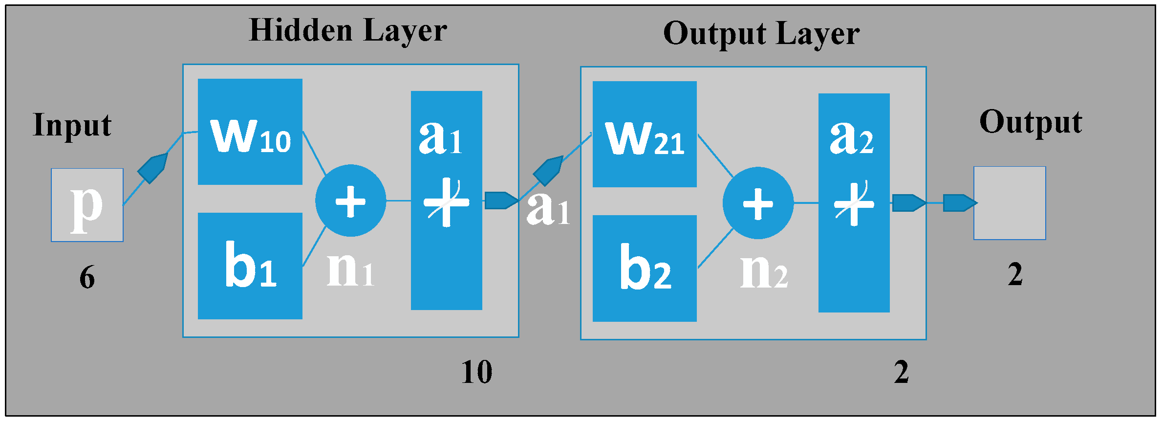
10], our gait classification neural network also has three layers in which the input layer has six neurons that correspond to the six input feature values. The hidden layer can automatically extract the features of the input patterns. There is no definite rule used to determine the number of neurons in the hidden layer; it is a hit-and-trial method. Here, in our classification study using ANN, there is one hidden layer holding 10 hidden neurons, the number of which was optimized by adjusting the size of hidden neurons (from 1 to 15) as shown in
Figure 10. For the hidden layer, a hyperbolic tangent sigmoid transfer function is used for each neuron. At the hidden layer, it is used to calculate network output from its input. The tangent hyperbolic function and its fast approximation are given by the following equation:
where
is the
i-th element of the
vector containing the output from the hidden neurons,
is the
i-th element of
vector containing the net input going into the hidden units and
is calculated by using the formula:
where
p is the input pattern,
is the bias vector and
is the weight matrix between the hidden layer and the output layer.
The output layer is designed based on the required output of the neural network. Here, we have used two output neurons corresponding to the two target classes the network needs to differentiate (i.e., the features of all patients are considered as Class 1, and all features of normal subjects are as Class 2). The pure linear activation function is selected for the output, given by the following equation:
where
is the column vector coming from the output layer and
is the output net inputs going into the output layer, which can be calculated by using the following formula:
Note here that b2 is the bias at the second layer; is the synaptic weights at the hidden layer and output layer; and a1 is the column vector containing the outputs from the hidden layer.
Here, we have used the back propagation learning algorithm that consists of two paths; the forward path and the backward path. The forward path includes creating the feed-forward network, initializing weights, simulation and training the network. The network weights and biases are updated in the backward path. Here, we have used the scaled conjugate gradient (SCG) training algorithm that uses the gradient of the performance function to determine how to adjust weights to minimize the performance function. An iteration of this algorithm can be written as:
where
is the vector of current weights and biases,
is the current gradient and
is the learning rate.
2.1.2. Support Vector Machine
The support vector machine (SVM) method is popular for performing pattern recognition/classification on two categories of data with supervised learning. In our work, SVM was implemented similar to [
10,
15,
16] to classify patients from normal subjects using the gait data from our WGAS system. A linear kernel was used for training the SVM classifier, which finds the maximum-margin hyper-plane from the given training dataset D, and it can be described as:
where
is either 1 or −1, and
n is the number of training data. Each
is a p-dimensional vector having the feature quantity
R. Any hyper-plane can be written as:
where
is the vector to the hyper-plane. If the training data are linearly separable, the hyper-plane can be described as [
15]:
The distance between these two hyper-planes is , so the purpose is to minimize .
In general, it is hard to separate the training data linearly. When the training data are not linearly separable, the hyper-plane can be described as:
where parameter C determines a trade-off between the error on the training set and the separation of the two classes. Here,
is a set of slack variables. The dual problems lie in maximizing the following function with respect to the Lagrange multiplier
[
15]:
subject to
:
2.1.3. K-Nearest Neighbor
The
K-nearest neighbors algorithm (KNN) is a simple, efficient non-parametric method used for classification and regression in pattern recognition, object recognition, etc. [
17]. In both cases, the input consists of the
K closest training examples in the feature space.
In KNN classification, the object or an unknown sample is classified by assigning to a test pattern the class label of its K nearest neighbors. The object is classified based on the category of its nearest neighbors through a voting procedure. Majority votes of its neighbors are considered during classification, with the object assigned to the most common class among its K nearest neighbors (K is a positive integer, typically small). If K = 1, then there is only one nearest neighbor, and the object is simply assigned to that class. Because of its simplicity and efficiency, the KNN-based algorithms are widely used in many applications.
2.1.4. Binary Decision Tree
Binary decision tree (BDT), also called as decision trees or classification trees, can predict responses to data as a classifier. To predict a response, one needs to follow the decisions in the tree from the root (beginning) node down to a leaf node, where the leaf node contains the response. BDT give responses that are nominal, such as “true” or “false”. Here, we have used BDT for the patients’ and normal subjects’ gait data classification. In data mining, BDT can also be used for regression and generalization of a given set of data [
18]. Data come in records of the form:
The dependent variable in Equation (14), Y, is the target variable that we are trying to predict, classify or generalize. The vector x consists of the input variables, x1, x2, x3, etc., that are used for classification.
The overall system flow for our real-time gait classification system is shown in
Figure 11. We will now present the classification results from our WGAS system using these aforementioned classifiers next.
3. Results and Discussion
The training and testing datasets were divided into 70:30 in percentages for the BP-ANN algorithm. The rest of the three algorithms used the
K-fold cross validation method with
K = 6 [
19]. The
K-fold cross validation method generalizes the approach by segmenting the data into
K equally-sized partitions. During each run, one of the partitions is chosen for testing, while the rest of them are used for training. The procedure is repeated
K times so that each partition is used for testing exactly once. Again, the total error is found by summing up the errors for
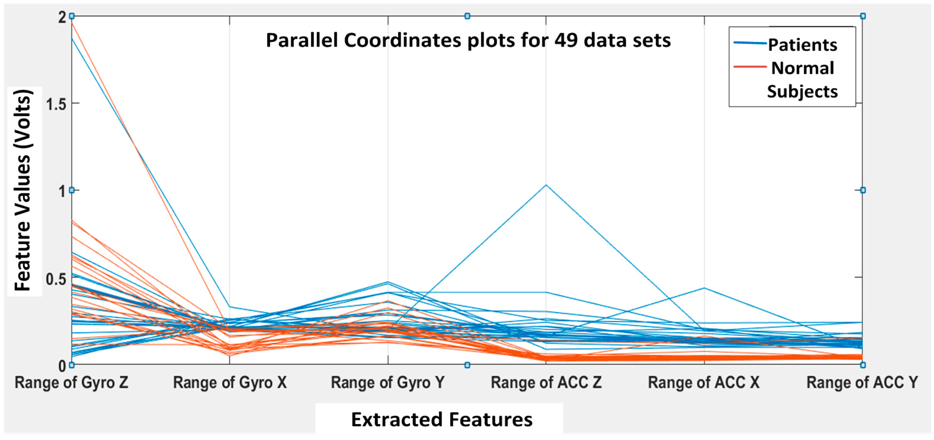
K runs. A parallel coordinate plot is shown in
Figure 12, illustrating the six features for all 49 datasets (seven subjects with seven DGI tests). The blue lines refer to extracted features for patients, and the brown lines refer to the extracted features for normal subjects.
From
Figure 12, we can clearly see that the features F4, F5 and F6 of the normal subjects (i.e., brown lines; range of ACC Z, range of ACC X and range of ACC Y, respectively) are almost concentrated at 0.1 Volts in the feature space, but the F4, F5 and F6 of the patients (i.e., blue lines) are varying from 0.2 to 1 in the feature space. Therefore, the linear acceleration features (i.e., F4, F5 and F6) from the accelerometer data can be used to differentiate patients from normal subjects. However, the gyroscopic features (i.e., F1, F2 and F3) vary rather differently, and they appear not that different for normal subjects vs. patients. Nevertheless, we found that the gyroscopic features are still important for the classification algorithms to possibly increase their classification accuracy.
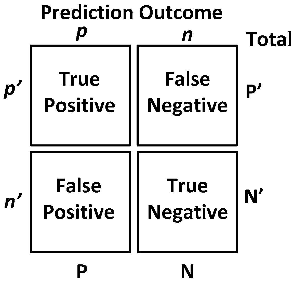
Before we show the classification results, we would like to introduce some straight-forward graphical representation and figures-of-merit used to evaluate a classifier. For example, a “confusion matrix” is a useful and simple tool for analyzing/representing how well a classifier can recognize input features of different classes [
20]. It tabulates the outcomes performed by a classifier for both correctly- and incorrectly-classified cases. Its definition is shown in
Figure 13.
Additionally, popular performance metrics for biosensors, such as sensitivity, specificity, positive predictive value (PPV) or precision, F-measure and accuracy, are also used in this work as defined below [
21], where TP = true positives, TN = true negatives, FP = false positives, FN = false negatives.
Sensitivity (recall): This measures the actual members of the class that are correctly identified as such. It is also referred to as the true positive rate (TPR). It is defined as the fraction of positive examples predicted correctly by the classification model.
Classifiers with large sensitivity have very few positive examples misclassified as the negative class.
Specificity: This is also known as the true negative rate. It is defined as the fraction of total negative examples that are predicted correctly by the model/classifier.
Precision (positive predictive value): Precision determines the fraction of records that actually turns out to be positive in the group the classifier has declared as positive class.
The higher the precision is, the lower the number of false positive errors committed by the classifier.
Negative predictive value (NPV): This is the proportion of samples that do not belong to the class under consideration and that are correctly identified as non-members of the class.
F − measure: Precision and sensitivity are two widely-used metrics for evaluating the correctness of a classifier or a pattern recognition algorithm. Building a model that maximizes both precision and sensitivity is the key challenge for classification algorithms. Precision and sensitivity can be summarized into another metric known as the F-measure, which is the harmonic mean of precision and sensitivity, given by,
Accuracy: Accuracy is used as a statistical measure of how well a binary classification test identifies or excludes a condition. It is a measure of the proportion of the true results as defined by Equation (20):
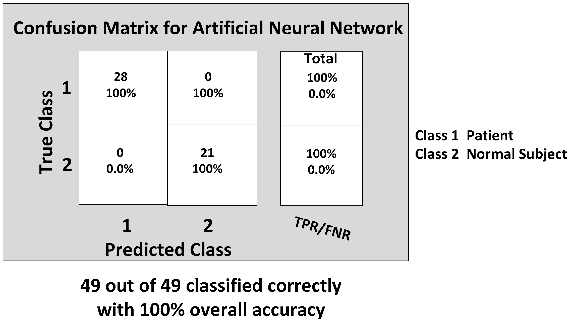
Now, we are ready to discuss the classification results. Considering the importance of all of these six features from the range data, each classifier was trained with the inputs of all six features. The back propagation artificial neural network (BP-ANN) achieved an impressive 100% accuracy with the SCG learning. This SCG algorithm performs the search and chooses the step size by using the information from the second order error function from the neural network. The SCG training is optimized by the parameter sigma σ (which determines the change in weight for the second derivative approximation) and lambda λ (which regulates the indefiniteness of the Hessian). The values of σ and λ were taken as and , respectively.
The confusion matrix of the BP-ANN classifier is shown in
Figure 14, which gives the TP, TN, FP and FN values.
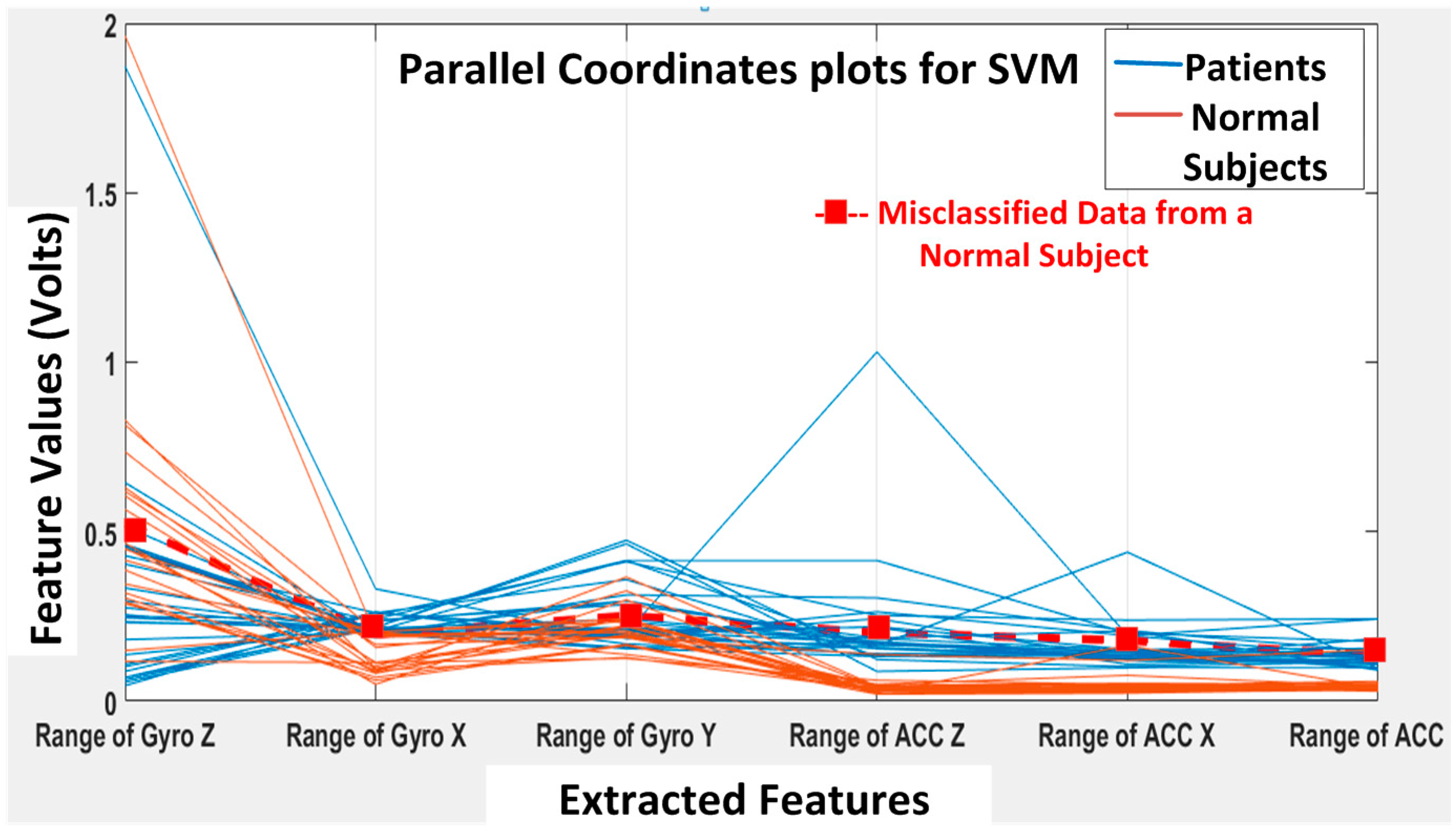
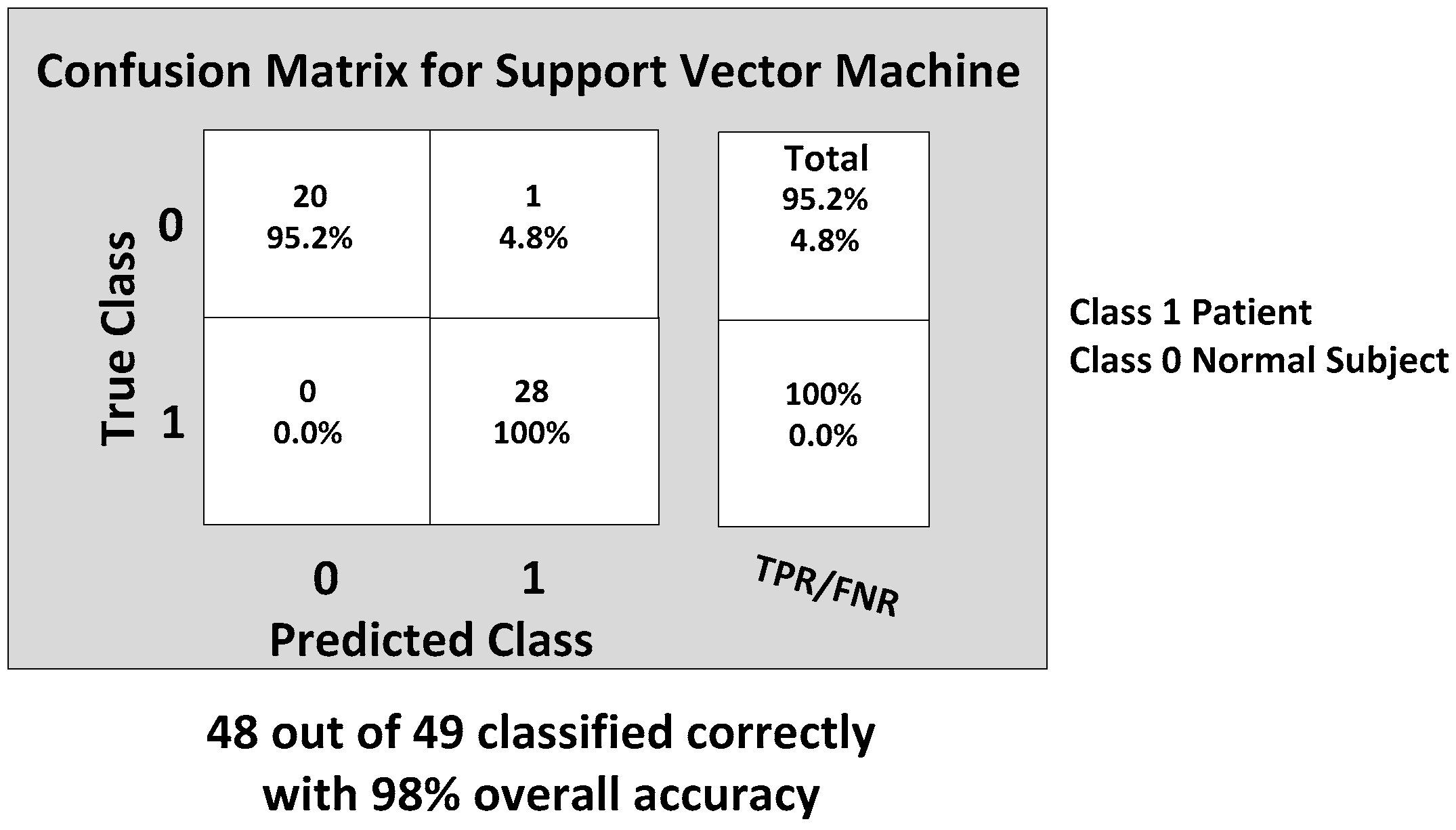
Next, the SVM classifier with a linear kernel achieved 98% overall accuracy with only one misclassification from the 49 feature datasets. The misclassified data are shown in
Figure 15, and the corresponding confusion matrix is shown in
Figure 16. The only one misclassification is Case 7 of the first normal subject, which was misclassified as the patient class.
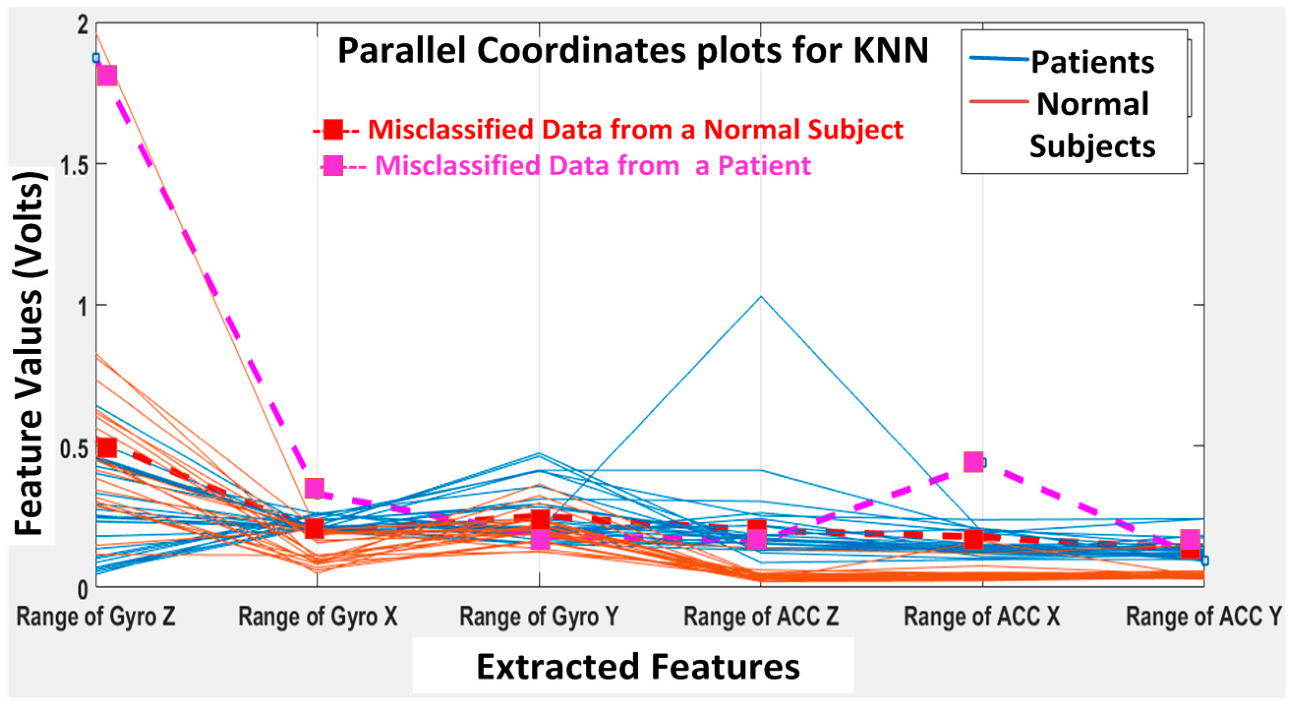
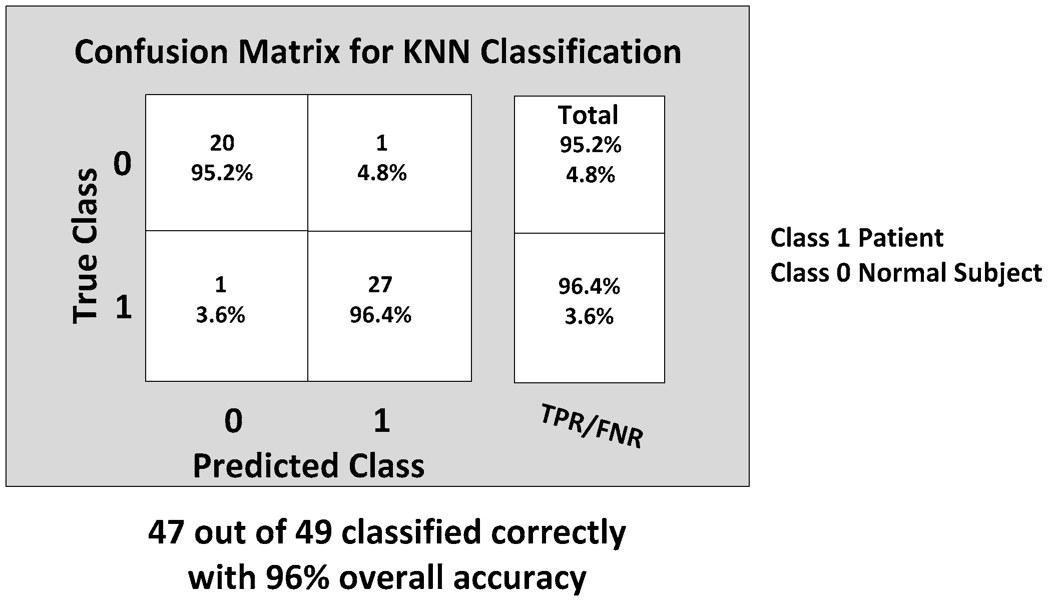
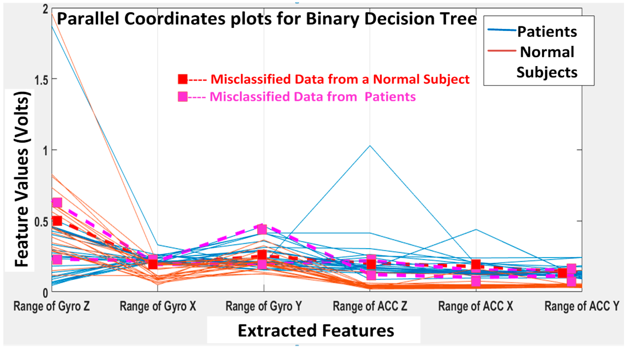
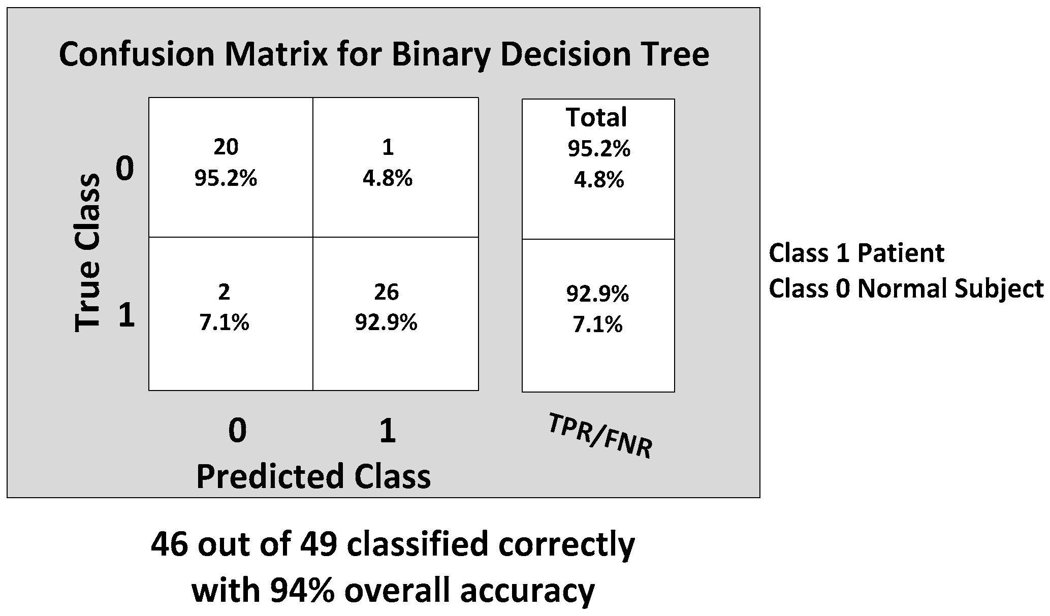
The KNN and BDT algorithms were also trained on the data collected and achieved 96% and 94% in accuracy, respectively. The parallel coordinates plots and the confusion matrices are shown in
Figure 17,
Figure 18,
Figure 19 and
Figure 20, respectively. For the KNN classifier, there are two misclassifications: Case 7 of the first normal subject and Case 1 of the second patient were misclassified. Somewhat similarly, for the BDT algorithm, there are three misclassifications: Case 7 of the first normal subject, Case 4 of the fourth patient and Case 6 of the first patient.
From the classification results of the trained algorithms, we can clearly see that our WGAS system is robust enough to differentiate patients and the normal subjects with the simple features extracted from the raw accelerometer and gyroscope data as each classifier exhibits 94%–100% high accuracy. The comparison and the performance of the algorithms are shown in the
Table 6 as below, where the range data have been used as the input features to the classifiers.
Next, we also tried different statistical parameters to use as the input features to check the impact on classifier accuracy. When only STDEV is used as the input feature,
Table 7 suggests the classification accuracies for all classifiers degraded, while SVM classification accuracy is now 94%, slightly better than the other classifiers. When both range and STDEV are used as the input features, the SVM’s accuracy improves to 98%, and all classifiers have higher than 94% accuracy. The best gait classification accuracy still occurs when only range data are used as input features; in that case, the BP-ANN outperformed all other classifiers with 100% accuracy.
Finally, we need to compare the running time of each of the classifiers to see which algorithm is the fastest to perform this gait classification in real time; we also compared the speed when different input features are used to train the classification algorithms, and the results are shown in
Table 8. It is apparent that a simple, but very fast BP-ANN classifier appears to be the best classifier to differentiate patients of balance disorders vs. the normal subjects in real time. SVM also has achieved 100% precision and specificity, but 98% accuracy; however, it is significantly slower than BP-ANN, KNN or BDT. We are collecting more gait data from patients and normal subjects now to improve the data statistics and to ascertain if BP-ANN and SVM would still be the best algorithms for real-time patient classification.
Table 9 shows the results of this work compared with previously-published work in the literature. The Mannini et al. [
22] used three IMUs featuring a tri-axial accelerometer and a tri-axial gyroscope and collected the raw data from the testing subjects. They have achieved 90.5% classification accuracy using the RBF (radial basis function) kernel SVM classification algorithm by including time domain features, like the mean value, STDEV, maximum, minimum and range in their feature extraction. The Tahir et al. [
23] used both ANN and SVM classifier algorithms for the gait classification in Parkinson’s disease patients. They have used the SVM classifier with the RBF kernel in distinguishing normal and patients based on kinetic features. They have also used ANN with the Levenberg–Marquardt training algorithm and achieved 98.2% and 96.9% classification accuracy, respectively.
The Bregg et al. [
24] applied an ANN and SVM for the automatic recognition of young-old gait types from their respective gait patterns. Minimum foot clearance (MFC) data of young and elderly participants were analyzed using a PEAK-2D motion analysis system during a 20-min continuous walk on a treadmill at a self-selected walking speed. Gait features extracted from Poincaré plot images were used to train the SVM and ANN. Cross-validation test results indicate that their generalization performance of the SVM was on average 83.3% (±2.9) to recognize young and elderly gait patterns, compared to a neural network’s accuracy of 75.0% (±5.0). The same research group of [
24] used a synchronized PEAK 3D motion analysis system and a force platform during normal walking for young and elderly subjects and achieved 83.3% vs. 91.7% generalization performance for ANN and SVM, respectively, as reported in [
25]. The Hasin et al. [
26] used both SVM and ANN for gait recognition by extracting geometry and texture features from the frame sequence of the video when the person is walking. They have used polynomial SVM of order three and BP-ANN with SCG training and achieved overall accuracy of 98% for both of the classifiers. The Huang et al. [
27] has built intelligent shoes for human identification under the framework of capturing and analyzing human gait. The data of that work were collected from different sensors, like a pressure sensor, a tilt angle sensor, three single-axis gyros, one tri-axial ACC and a bend sensor installed in the shoe. Principle component analysis (PCA) was used for feature generation, and SVM was applied for training and classifier generation. They were successful in achieving a 98% human identification rate. The Lugade et al. [
28] used ANN to determine dynamic balance control, as defined by the interaction of the center of mass (CoM) with the base of support (BoS), during the gait in the elderly using clinical evaluation on gaits. Subjects were asked to walk at a self-selected comfortable speed across a 10 m walkway in that work. During ambulation, 29 retro reflective markers were placed on bony landmarks of the body, where 3D marker trajectories were captured with an eight-camera motion analysis system (Motion Analysis Corp, Santa Rosa, CA, USA). BP-ANN was able to correctly identify the interaction of the CoM with BoS of elderly subjects with an 89% accuracy rate.
The Muhammad et al. [
29] used 25 reflective markers, which were placed on the body, and data were acquired from the Vicon Nexus 3D motion capture system to analyze the gait patterns, kinetic and kinematic parameters of the hip, knee and ankle joints of patients and normal subjects. They have used ANN to predict the gait patters with approximately 95% accuracy. The Ahlrichs et al. [
30] used one tri-accelerometer device worn on the waist of the testing subjects used in detecting the freezing of gait (FOG) symptoms on the people suffering from Parkinson’s disease. The acceleration signals from a waist-mounted sensor are split into equally-sized windows (i.e., a sliding window is applied to the time series), and features are extracted from those windows and fed to an SVM for training or classification. The RBF kernel SVM achieved 98% accuracy in detecting the symptoms for the patients with Parkinson’s disease.
We have attempted to validate the measured WGAS data with the data taken from a video-based kinematic reference system; i.e., a Vicon motion capture system with cameras. However, so far, we have found it very difficult to validate the WGAS data directly this way, as the Vicon camera-based system measures the movements from the markers on the body, but not the exact force-based acceleration data, as measured from our WGAS. Therefore, a limitation of the current paper exists in the lack of a direct validation of the values of the extracted features to the measured data provided by another reference system (e.g., a kinematic system). However, we do plan to continue the next stage of the research by including this validation step against possibly another kinematic system and/or using a different validation method. In addition, to improve the data statistics of our work, we would like to add more data as we compared the performance of the classifiers with the increased normal data, as shown in
Table 10 in the revised manuscript. The total dataset has four patients and twelve normal subjects, and the overall accuracies are still improved when compared with the results from
Table 6.


