Smart Structural Health Monitoring of Flexible Pavements Using Machine Learning Methods

Abstract

The pavement is a complex structure that is influenced by various environmental and loading conditions. The regular assessment of pavement performance is essential for road network maintenance. International roughness index (IRI) and pavement condition index (PCI) are well-known indices used for smoothness and surface condition assessment, respectively. Machine learning techniques have recently made significant advancements in pavement engineering. This paper presents a novel roughness-distress study using random forest (RF). After determining the PCI and IRI values for the sample units, the PCI prediction process is advanced using RF and random forest trained with a genetic algorithm (RF-GA). The models are validated using correlation coefficient (CC), scatter index (SI), and Willmott’s index of agreement (WI) criteria. For the RF method, the values of the three parameters mentioned were −0.177, 0.296, and 0.281, respectively, whereas in the RF-GA method, −0.031, 0.238, and 0.297 values were obtained for these parameters. This paper aims to fulfill the literature’s identified gaps and help pavement engineers overcome the challenges with the conventional pavement maintenance systems.

1. Introduction

The pavement network plays a critical key in today’s mobility and transportation. It is a complex and dynamic structure influenced by various environmental and loading conditions [1]. Regular pavement maintenance is a far more cost-effective approach than reconstructing it because of improper maintenance [1]. The pavement network requires constant maintenance and repair due to gradual deterioration induced by factors such as pavement aging and increased traffic flow [2]. Maintaining the desired service level of a pavement network requires constant evaluation. According to Moghadas Nejad and Jahanshahi et al. [3,4], the common pavement condition assessment methods can be categorized as follows:

• Assessment of the pavement Roughness (determining ups and downs)
• Assessment of surface conditions (determining surface distresses)
• Assessment of the pavement structural condition (determining the load capacity)
• Assessment of pavement safety condition

Today, new methods and equipment have been developed for pavement assessment. Countries like the US, which have appropriate and sufficient financial resources, are leading in such fields. In these countries, the methodologies used in different states may even differ because each state has enough technical and financial capacity to research, develop, and provide its unique equipment and methodologies. For example, states like Texas, Virginia, and Maryland use different approaches to pavement condition. In contrast, countries like Iran have severe technical and budget limitations. These limitations cause that new technologies have not been made available to Iranian engineers. As an example, there is no enough number of fully equipped laboratories in Iran. Most transportation departments of Iran have not any non-destructive device. They often are equipped with a basic asphalt and bitumen testing laboratory. Also, the lack of skilled and trained staff familiar with new technologies is another problem in Iran. As a result, the old methods of evaluating the pavement are still used in Iran. For instance, Iranian engineers still evaluate pavement surface conditions with the help of visual examination by an inspector. In such conditions, the authors think that the best idea is to maximize the use of existing equipment and methods. The pavement condition index (PCI) and the international roughness index (IRI) are the two critical indices in monitoring flexible pavements’ structural health in Iran. IRI is a numerical index provided by the World Bank. This index is derived from dividing roughness by the longitudinal distance [5,6,7,8]. IRI is a symbol for the longitudinal roughness of roads. The lower values of IRI indicate higher quality. As an example, a pavement with IRI equal to zero has the ideal condition [9,10]. PCI is another numerical index for the evaluation of the pavements. This index rates the pavement with a number between 0 (worst condition) to 100 (perfect condition). Initially, each pavement is assigned with a score of 100. Then, the score subtracted based on the type, severity, and extent of distresses [11,12]. In fact, IRI represents the pavement roughness, and PCI is the representative of pavement distresses. The surface roughness of pavement is a primary concern for users, drivers and passengers [13,14]. The roughness intensifies the vertical stresses on the pavement and exacerbates pavement fatigue. Also, it can be considered as a factor for aggravating pavement distresses. Moreover, the roughness unravels deformations in the pavement surface. This issue influences road drainage and driving safety [15]. On the other hand, any pavement distress will deteriorate the pavement roughness [16]. As a result, it can be concluded that there is a causal, bilateral, direct relationship between the distresses and roughness in pavements [17,18].

On the other hand, the modeling achievements enable engineers to study physical systems located in their environment without the need to implement all traditional testing approaches [19]. In pavement engineering, there are many variables and complex systems that affect one another. Therefore, pavement researchers are less likely to use simple statistical methods for creating pavement prediction models. Also, the nonlinear shape of the pavement performance curve intensifies this unwillingness [20]. Consequently, studies have attempted to apply machine learning (ML) techniques to develop more accurate models [21]. Modeling and using ML techniques can help engineers replace traditional approaches. Therefore, the authors aimed to overcome the mentioned challenges for Iranian engineers with the help of machine training methods and pavement modeling.

This paper focuses on the assessment and modeling of roughness and surface conditions in flexible pavements. Actually, this study’s primary objective is to develop a new method for replacing the traditional methods in determining PCI. The results of roughness and surface condition assessment of the Tehran-Qom Freeway in Iran were used in this study to proceed with the proposed theory. In this freeway, at 2-km intervals, a 100-m sample unit was selected from the slow-speed lane. For each sample unit, IRI was calculated by road surface profiler (RSP), and PCI was determined from the inspection of surface distresses. The proposed theory was developed by analyzing IRI and PCI values with the help of random forest (RF), and random forest optimized by genetic algorithm (RF-GA) methods. For validation of the results, correlation coefficient (CC), scatter index (SI), and Willmott’s index of agreement (WI) criteria was utilized. The proposed method can improve the maintenance process of pavements in Iran. Additionally, this method can reduce or remove old techniques for determining PCI, such as financial resource limitations, shortage of skilled inspectors, labor and time consumption, and safety issues for inspectors and users. In Section 2, authors provide a bstate of the art literature review. The research methodology is delineated in Section 3. Section 4 includes the results and discussion. Finally, the conclusion is presented in Section 5.

2. Background

Numerous studies have been conducted in the field of simultaneous assessment of the surface conditions and roughness in pavements, which will be reviewed below. In 1989, Sharaf and Hanno conducted one of the oldest studies on the relationship between IRI and PCI [22]. The final model of their study was the following simple equation.

$$\mathrm{PCI}=100-\left(6.667\times \mathrm{IRI}\right)$$

(1)

As can be seen in Equation (1), they proposed a first-order linear equation for the relationship between IRI and PCI. This equation was later used in the master of science thesis by Abd-Allah [23], as well as another paper by Sharaf [24].

In 2002, Dewan and Smith introduced another equation for the prediction of IRI based on PCI. Their study was related to the Bay Area cities and counties, in California. The coefficient of variation and R² were 28% and 0.53, respectively, which depicts a low correlation [25]:

$$\mathrm{PCI}=153-\left(58.48\times \mathrm{IRI}\right)$$

(2)

Park et al. (2007) undertook a study to investigate the relationship between surface distress and roughness in asphalt pavements. They presented a power regression model for the association between IRI and PCI [18]:

$$\mathrm{PCI}={\mathrm{K}}_1\times {\mathrm{IRI}}^{{\mathrm{K}}_2}$$

(3)

where K₁ and K₂ are regression coefficients. Park et al. calibrated this model for pavement sections in the North Atlantic region and obtained the values of 100 and −0.436 for K₁ and K₂, respectively.

Arhin et al., drawing on data derived from the District Department of Transportation, which were collected from 2009 to 2012, presented a calculating PCI model using IRI in dense urban areas. This relation is as follows [26]:

$$\mathrm{PCI}=\mathrm{A}\times \left(\mathrm{IRI}\right)+\mathrm{K}+\mathsf{\epsilon }$$

(4)

where A and K are constant coefficients, and $\mathsf{\epsilon }$ is the model error.

The above model’s coefficients are calculated based on the road functional classification and type of pavement, as shown in

Table 1. Prediction of PCI for various road functional classifications.

Model Form	Road Functional Classification
PCI = −0.215(IRI) + 110.73	Freeways
PCI = −0.206(IRI) + 114.15	Arterials
PCI = −0.217(IRI) + 115.32	Collectors
PCI = −0.186(IRI) + 110.31	Locals

and

Table 2. Prediction of PCI for various pavement type.

Model Form	Pavement Type
PCI = −0.224(IRI) + 120.02	Asphalt
PCI = −0.203(IRI) + 113.73	Composite
PCI = −0.172(IRI) + 110.01	Concrete

. These tables are adapted from the study of Arhin et al. [26].

Elhadidy et al. (2019) presented a sigmoid relationship between IRI and PCI. In this study, A total of 1448 sections from LTPP were used for the model construction [27]. The proposed model by them was presented in Equation (5).

$$\mathrm{PCI}=\frac{1}{0.048}\times \ln (\frac{79.933}{\mathrm{IRI}}-14.061)$$

(5)

Similar to Sharaf and Hanno, Ali et al. (2019) developed a regression model using the statistical program SPSS. They used a dataset from St. John’s road network includes over 1000 km of paved roads [28].

$$\mathrm{PCI}=81.89-\left(11.037\times \mathrm{IRI}\right)$$

(6)

On the other hand, the application of ML methods in civil engineering is constantly increasing. Pavement engineering, as one of the branches of civil engineering, is no exception to this rule. Predicting indicators of pavement quality control programs (QCP) is one of the most important topics in which ML methods have been used. Many researchers have tried to study, analyze, and model indicators, such as IRI, PCI, alligator deterioration index (ADI), etc. using ML methods. Often the goal of these researchers was to optimize the traditional approaches in pavement management systems. Here are some of these efforts. Marcelino et al. used the RF method to predict IRI [29]. In several studies, Hoang et al. used ML techniques such as support vector machine (SVM), artificial neural network (ANN), RF, radial basis function neural network (RBFNN), naïve Bayesian classifier (NBC), and classification tree (CT), along with image processing techniques to investigate and identify pavement cracks [30,31,32]. In Iran, Moghadas Nejad et al. Focused on the characterization of laboratory-made asphalt concrete samples using image processing and ANN techniques [33,34]. Fathi et al. used a hybrid car training method that was a combination of RF and ANN methods to predict the ADI index [35].

Souza et al. proposed a low-cost pavement condition assessment system based on data collected by smartphone accelerometer sensors and ML methods [36]. Nabipour et al. used SVM and genetic expression programming (GEP) methods to predict the remaining service life (RSL) pavement [37]. Similar to Hoang’s studies, Fujita et al. used ML methods to identify asphalt pavement cracks. They used a linear support vector machine as the classifier [38]. By using the multi-layer perceptron (MLP), SVM, and RF methods, Nitsche et al. tried to estimate weighted longitudinal profile (WLP) indices. Their purpose was to evaluate the efficiency of these methods in the process of predicting range and standard deviation [39]. Karballaeezadeh et al. utilized an optimized SVM to estimate RSL in flexible pavements. They optimized SVM with the help of a particle filter. The results showed that this optimization greatly improved the SVM prediction quality, and the results were even better than the MLP results [40]. In another study, Karballaeezadeh et al. applied three methods, Gaussian process regression (GPR), M5P model tree, and RF, for prediction of the structural capacity in flexible pavements. Their target parameter was the structural number (SN) [41]. Inkoom et al., with the help of ML methodologies, tried to predict highway pavement conditions. They employed bootstrap forest, gradient boosted trees, K nearest neighbors, Naïve Bayes, and multivariable linear regression methods [42]. Zeiada et al. used ML methods to model pavement performance in the warm regions. First, the most important design factors in warm regions were identified using an ANN supported by a forward sequential feature selection algorithm. Then, they performed the modeling process using GPR, SVM, ensemble, ANN, and regression tree methods [43]. Cao et al. applied ANN and SVM methods to model acoustic longevity. Their modeling inputs included maximum aggregate size, binder content, air void content, vehicle speed, and thickness extracted from 270 asphalt pavement sections in Hong Kong [44]. The above-mentioned studies, which are only part of the research done using ML methods, show that the use of these techniques in pavement engineering is increasing rapidly.

An accurate and comprehensive investigation of the literature review can help researchers to find the existing potential gaps. After a broad review of related conducted studies, the authors notice that there are two main gaps. (1) Although many researchers have focused on the use of artificial intelligence (AI) techniques in pavement engineering, no specific study has been conducted to investigate the relationship between PCI and IRI with the help of RF and GA. (2) Traffic and loading patterns, weather conditions, quality and quantity of maintenance systems, etc. can be different from one country to another. Therefore, for the effective implementation of pavement management programs, it is better to assess any country’s pavement networks independently. Among previous studies, no study has been conducted based on data extracted from Iranian roads. Therefore, Iranian engineers should always calibrate such models for the conditions of Iran. As a consequence, the authors were encouraged to study the relationship between PCI and IRI in Iran using RF and GA techniques. This paper’s novelty can be found in using the RF and GA techniques for predicting PCI-based IRI. Also, implementing this idea for a case study in Iran is another novelty in this study.

3. Materials and Methods

3.1. Pavement Qualitative Indices

The pavement distress is caused by traffic (loading) and environmental factors when a road is in-service. Even in an experimental pavement section, which is not subject to traffic, distresses appear after a while as a result of environmental factors [45]. Therefore, pavement distress is a critical issue that should be considered by engineers during the maintenance period. For the effective maintenance of pavement, engineers often use surface quality indicators. Each qualitative index, defined based on certain distresses, indicates pavement quality at the time of inspection. Therefore, suitable indices allow pavement engineers to plan, prioritize, and allocate road maintenance budgets [11]. Section 3.1.1 and Section 3.1.2 introduce two important indices for pavement maintenance named PCI and IRI.

3.1.1. Pavement Condition Index (PCI)

One of the most recognized qualitative indices of pavement presented by the US Army’s engineering department in the late 1970s is PCI [46]. The PCI is a numerical index that evaluates pavement conditions based on pavement surface distresses and demonstrates structural integrity and surface operational conditions. This index’s value varies from zero to 100, with zero representing the worst conditions and 100 showing perfect conditions [11,47]. ASTM D6433-18 [48] evaluates pavement condition based on PCI, as displayed in

Table 3. The rating scale of PCI.

PCI Range	0–10	10–25	25–40	40–55	55–70	70–85	85–100
Evaluation	Failed	Serious	Very poor	Poor	Fair	Satisfactory	Good

. adapted from [48].

For each pavement sample unit, the maximum PCI value (100) is initially allocated and then based on pavement surface condition, the maximum corrected deduct value (CDV) is deducted from 100 (see Equation (7)) [48]:

$$\mathrm{PCI}=100- {\mathrm{CDV}}_{\max }.$$

(7)

where CDV_max is the maximum of CDV based on type, severity, and extent of distresses. For each type of distress, the deduct specific curves measure values (DVs). Then, the number of DVs is diminished to the maximum number allowed, and also the number of DVs greater than 2 (q) is determined. Finally, CDV can be calculated by using q, TDV (sum of DVs), and related curves. Readers can refer to ASTM D6433-18 [48] for more details.

3.1.2. International Roughness Index (IRI)

Effective maintenance of the pavement network to ensure transportation safety requires awareness of the pavement surface’s surface [49]. In pavement management systems (PMSs), surface roughness data is used for planning at the project level and the network level. This data is utilized at the project level for quality control during the pavement construction phase, and the determination of areas with excessive roughness. However, roughness data is used to determine the permissible roughness limits at the network level, divide the pavement network into uniform pieces, and prioritize maintenance operations [11,50]. Roughness data is important in road safety analysis methods as well [51]. All types of pavement have roughness. Even in newly constructed pavements that have not been exposed to the traffic load, there may be some roughness due to inappropriate execution quality. Generally, pavement roughness increases as a result of traffic loading and environmental conditions [11,52].

The most common index of longitudinal roughness of pavements and the driving quality is the IRI, which has been introduced and used for nearly three decades. This indicator was proposed by the World Bank in 1982, based on the international road roughness experiment (IRRE) [53,54]. IRI is a quantitative index of pavement smoothness, which in addition to driving quality, determines the pavement performance [49,53,55]. IRI is based on a quarter-car system (QCS) simulation driving at a speed of 80 km/h [11,49]. Figure 1, adapted from the studies of Sayers [56] and Zoccali et al. [57], shows the quarter-car system.

IRI is the average rectified slope, which is generally expressed in terms of mm/m or m/km [49,58]:

$$\mathrm{IRI}=\frac{1}{\mathrm{L}}{{\displaystyle \int }}_0^{\frac{\mathrm{L}}{\mathrm{V}}}\left|\dot{{\mathrm{Z}}_{\mathrm{s}}}-\dot{{\mathrm{Z}}_{\mathrm{u}}}\right|\mathrm{dt}=\frac{\mathrm{The}\mathrm{accumulated}\mathrm{suspension}\mathrm{vertical}\mathrm{motion}}{\mathrm{The}\mathrm{distance}\mathrm{traveled}\mathrm{during}\mathrm{the}\mathrm{test}}$$

(8)

where Z(X) is the longitudinal profile, K_s is suspension spring rate, K_t is tyre spring rate, C_s is suspension damping rate, m_u is unsprung mass, and m_s is sprung mass. According to the Federal Highway Administration (FHWA) [59], in-service pavements can be evaluated based on the IRI value, as shown in

Table 4. Evaluation of Road Pavement According to IRI.

IRI (m/km)		Ride Quality
Interstate Highways	Other Highways
<0.95	<0.95	Very good
0.95–1.50	0.95–1.50	Good
1.50–1.89	1.50–2.69	Fair
1.90–2.70	2.70–3.48	Mediocre
>2.70	>3.48	Poor

. adapted from [59].

3.2. Case Study

The pavement sections investigated in this paper were selected from both directions of the Tehran-Qom Freeway. Tehran-Qom freeways is the most crucial freeway in Iran. The right of way for this freeway is considered more than other Iranian roads. Furthermore, this freeway is one of Iran’s North-South national corridor’s main sections, which is regarded as the entrance to the capital (Tehran). Therefore, the Authors selected this freeway for their research. The freeway’s total length is 236 km, which comprises two 118-km routes from Tehran to Qom and vice versa. This freeway has 3 lanes in each direction, with a width of 3.65 m per lane. It is further divided into two branches of Tehran-Qom and Qom-Tehran. The sample units under study, which are 100 m in length and 3.65 m in width, were selected at 2-km intervals from the slow-speed lane. After field inspection of sample units, the surface distress conditions were determined, and the results are presented in

Table 5. Surface Distresses in Tehran-Qom freeway.

Tehran-Qom Branch		Qom-Tehran Branch
Type of Distress	Percentage of Whole Distress	Type of Distress	Percentage of Whole Distress
Raveling	53.01	Block cracking	41.78
Block cracking	26.40	Raveling	34.75
Rutting	12.59	Alligator cracking	10.02
Alligator cracking	4.05	Bleeding	8.71
Polished aggregate	2.05	Patching	1.73
Bleeding	1.46	Rutting	1.67
Patching	0.42	Polished aggregate	1.28
Shoulder separation	0.01	Depression	0.06

and

Table 6. Longitudinal Distresses in Tehran-Qom Freeway.

Tehran-Qom Branch		Qom-Tehran Branch
Type of Distress	Percentage of Whole Distress	Type of Distress	Percentage of Whole Distress
Longitudinal and transverse cracking	94.61	Longitudinal and transverse cracking	99.28
Shoulder drop-off	5.25	Joint reflection cracking	0.36
Corrugation	0.09	Corrugation	0.31
Edge cracking	0.05	Shoulder drop-off	0.05

. For each sample unit, PCI was calculated using the method presented in the ASTM D6433-18 standard [48].

In the next step of pavement condition assessment, sample units are investigated by a two-laser RSP device (TSML, Tehran, Iran), and the IRI index is calculated per unit. The IRI of each unit is the average IRI of that unit. Figure 2 shows the RSP device. This device uses a line laser system for determining IRI in wheels paths (Figure 3). The laser sensors are installed in a rigid aluminum housing placed at the front of the vehicle. The driver of the vehicle controls the RSP systems. The RSP collects data at a speed of around 110 km/h. RSP receives and stores data using a computer. A program receives all processed data, displays it on the computer screen, and stores the hard disk data. The RSP is capable of determining pavement roughness in roads and airports. Along the longitudinal axis, the RSP measures the pavement profile. This profile contains information such as roughness, grade, and coarse texture. The longitudinal profile of the pavement can be measured along any hypothetical line along the pavement axis. The most important longitudinal profile is parallel to the vehicle’s wheels, which transmits the roughness to the driver. Today, however, civil engineers use new equipment for checking surface quality, such as the light detection and ranging (LiDAR) system [60,61,62]. This 3D laser scanning system (TSML, Tehran, Iran) can provide a three-dimensional profile of the pavement surface. In addition to roughness, these devices can collect other useful information from the pavement’s surface, such as the type, severity, and quantity of surface damage.

3.3. Analysis Phase by Using Machine Learning

This section is related to the application of ML in the proposed theory. In recent years, the application of ML methods in engineering sciences is widespread. A machine learning method such as RF has received much attention from engineers [29,41,63,64]. This volume of RF usage in transportation research shows that this engineering field has entered a new study phase. In this phase, researchers are looking to use ML techniques to improve transportation engineering processes. This could be a turning point in transportation engineering. However, the multiplicity of ML methods used by researchers can indicate an important issue: What is the most ideal and accurate method of ML? Does this study phase have a big gap? According to the authors, the introduction of new algorithms suggests that ML still has a lot of work to do to impact the transportation industry. This prompted the authors to use ML methods in their research. In the authors’ proposed theory, ML helps to improve and enhance the inspection process of pavements. Therefore, after the necessary examinations, the authors chose the following two methods for their study to predict PCI based on IRI:

• Random forest (RF)
• Random forest optimized by genetic algorithm (RF-GA)

These methods are introduced in the next sections.

3.3.1. Random Forest (RF)

As an ensemble ML algorithm, RF uses many regression trees for the prediction process [41,64,65,66,67,68]. This algorithm was proposed by Breiman in 2001 and belonged to the ensembled learning method [67,69]. Ensemble classification methods have passed the test of time and proved to be highly accurate prediction and classification techniques [70]. The ensemble learning method’s main idea is to construct and combine the multiple base learners for obtaining better general abilities [71]. To create these learners, different training sets from the population should be utilized. RFs use bootstrap to build multiple training data sets. Bootstrap is a sampling method used to replace the scenarios from the constructed populations’ training subset during the analysis. After the training sets are ready, the algorithm trains a base learner on each of these sets. The final models are averaged, and the different outputs are merged into a unique estimation [37,72]. RFs are able to overcome the overfitting of regression trees [37,73]. RFs need two parameters to be tuned, including the number of regression trees (ntree) and the number of different predictors in each node (mtry) [35,66,73,74,75,76,77]. These two most critical parameters define the performances of RFs. Therefore, the choice of these two parameters is very important. Figure 4 shows the RF process. The models are implemented using the standard Mathworks’ statistics and machine learning toolbox version 11.0 integrated with the parallel computing toolbox version 6.9.

3.3.2. Random Forest Optimized by Genetic Algorithm (RF-GA)

Developed by Holland (1992) and Goldberg (1989) [78], GA is a general-purpose optimization search algorithm based on Darwin’s natural selection and genetic theory in biological systems [79,80]. These algorithms are inspired by some biological evolution mechanisms such as selection, crossover, and mutation [78,79,80,81,82]. The typical form of GA includes three steps [78,79,81]:

• Initial population generation
• Computation of fitness
• Construction of the new generation

First, GA produces an initial population or generation with each individual solution. Then, GA examines the goodness of the solution using a designed fitness function. This fitness function’s value identifies the current population’s survivors, representing the parents for the following population. In step 3, GA generates the new generation by the selection, crossover, and mutation processes. The next step is to repeat steps 2 and 3. This repetitive process is held until the highest number of generations or the desired accuracy is achieved [79,81,83,84].

As explained earlier, ntrees and mtry are the two most crucial parameters that determine the performance of RFs. Therefore, the aim is the optimization of these two parameters. In this study, GA is used to optimize these parameters. With the help of GA, authors put forward a new algorithm for predicting PCI, using GA to search the decision tree of RF and generate the most beneficial decision tree combination, so that the precision of integrated classification is promoted. These decision tree knots are eventually synthesized into the new integrated classifier.

In brief, present study introduces a RF algorithm based on GA optimization. This algorithm combines RF and GA, namely RF-GA, to choose the optimal combination of classification parameters. The core parameters of RF-GA proposed in this paper include the number of trees, maximal depth, confidence, minimal leaf size, minimal size for split, number of preparing alternatives, and subset ratio.

3.4. Validation of the Modeling

Three performance evaluations, i.e., correlation coefficient (CC), scatter index (SI), and Willmott’s index of agreement (WI), are used. Equations (9)–(11) [37] describe these methods as follows.

$$\mathrm{CC}=\frac{{{\displaystyle \sum }}_{\mathrm{i}=1}^{\mathrm{n}}{\mathrm{PCI}}_{\mathrm{Oi}}{\mathrm{PCI}}_{\mathrm{Pi}}-\frac{1}{\mathrm{n}}{{\displaystyle \sum }}_{\mathrm{i}=1}^{\mathrm{n}}{\mathrm{PCI}}_{\mathrm{Oi}}{{\displaystyle \sum }}_{\mathrm{i}=1}^{\mathrm{n}}{\mathrm{PCI}}_{\mathrm{Pi}}}{\left({{\displaystyle \sum }}_{\mathrm{i}=1}^{\mathrm{n}}{\mathrm{PCI}}_{\mathrm{Oi}}{}^2-\frac{1}{\mathrm{n}}{\left({{\displaystyle \sum }}_{\mathrm{i}=1}^{\mathrm{n}}{\mathrm{PCI}}_{\mathrm{Oi}}\right)}^2\right)\left({{\displaystyle \sum }}_{\mathrm{i}=1}^{\mathrm{n}}{\mathrm{PCI}}_{\mathrm{Pi}}{}^2-\frac{1}{\mathrm{n}}{\left({{\displaystyle \sum }}_{\mathrm{i}=1}^{\mathrm{n}}{\mathrm{PCI}}_{\mathrm{Pi}}\right)}^2\right)}.$$

(9)

$$\mathrm{SI}=\frac{\sqrt{\frac{1}{\mathrm{n}}{{\displaystyle \sum }}_{\mathrm{i}=1}^{\mathrm{n}}{\left({\mathrm{PCI}}_{\mathrm{Pi}}-{\mathrm{PCI}}_{\mathrm{Oi}}\right)}^2}}{\overline{{\mathrm{PCI}}_{\mathrm{Oi}}}}.$$

(10)

$$\mathrm{WI}=1-\left[\frac{{{\displaystyle \sum }}_{\mathrm{i}=1}^{\mathrm{n}}{\left({\mathrm{PCI}}_{\mathrm{Pi}}-{\mathrm{PCI}}_{\mathrm{Oi}}\right)}^2}{{{\displaystyle \sum }}_{\mathrm{i}=1}^{\mathrm{n}}{\left(\left|{\mathrm{PCI}}_{\mathrm{Pi}}-\overline{{\mathrm{PCI}}_{\mathrm{Oi}}}\right|+\left|{\mathrm{PCI}}_{\mathrm{Oi}}-\overline{{\mathrm{PCI}}_{\mathrm{Oi}}}\right|\right)}^2}\right].$$

(11)

where PCI_Oi, PCI_Pi, $\overline{{\mathrm{PCI}}_{\mathrm{Oi}}}$, and n are ith observed PCI, ith PCI predicted by the model, mean of observed PCI values, and the number of observed PCI values, respectively.

CC is a statistic that measures the linear correlation between observed and predicted PCIs. The values of CC are between +1 and −1. A value of +1 is a positive (direct) correlation, 0 is no correlation, and −1 is a negative (inverse) correlation. Whatever the CC value is closer to +1 or −1, the accuracy of predictions is higher. SI is calculated by dividing root mean square error (RMSE) with the mean of the observed PCIs. In fact, SI is an index that shows errors. When the SI value is closer to 0, the accuracy of predictions is higher. As an index of agreement, WI was proposed by Willmott (1981).

WI is a standardized measure of the degree of model prediction error. This index reflects the degree to which the simulated variate accurately estimates the observed variate. WI is a measure of the degree to which a model’s predictions are error free. This index varies between 0 and 1. The WI of 1 indicates perfect agreement between observed and predicted data, and 0 indicates no agreement at all [37].

4. Results

Analysis methods, namely RF and RF-GA, were presented in Section 3.3. This section represents the results of methods. Statistical characteristics of IRI and PCI indices are presented in

Table 7. Statistical characteristics of the utilized data.

Variable	Mean	Min.	Max.	Std. Deviation	Skewness	Kurtosis	Sig. in Kolmogorov–Smirnov Test	Correlation with PCI
IRI	1.843	0.98511	3.600	0.5255	0.797	0.778	0.049	−0.15
PCI	72.746	7.000	100.000	18.6057	−0.904	1.399	0.003	1

. The data was extracted from IBM SPSS 23 software (version 2015, International Business Machines Corporation (IBM), Armonk, New York, NY, USA).

The mean IRI is 1.843. Therefore the average condition of all sections is fair (see Table 4). On the other hand, the mean PCI, 72.746, shows that all sections’ average condition is satisfactory (see Table 3). Standard deviation is one of the scattering indices that shows how far the average data is from the mean [85,86]. For calculating the correlation coefficient, the first step is to determine the normality status of data. Therefore, the skewness, kurtosis, and significance level in the Kolmogorov–Smirnov test were calculated. Based on the literature, when the skewness and Kurtosis values are between 2 and −2, the data distribution is considered normal. As a non-parametric test, Kolmogorov–Smirnov helps to determine if the data is normal or not. In this test, data is normal when the significance level (sig.) is above 0.05 [37,86]. So, Table 7 confirms IRI had better normal distribution than PCI. Also, both IRI and PCI are non-normal because of their sig. are less than 0.05.

The adopting of the test type for correlation is based on normality condition. even if one of the variables is non-normal, then the Spearman test is used [86]. The correlation between IRI and PCI is 15%, which represents a weak value.

RF has seven main parameters including the number of trees (A), maximal depth (B), confidence (C), minimal leaf size (D), minimal size for split (E), number of prepruning alternatives (F), and subset ratio (G). The quality of RF performance depends on the value of these parameters.

Table 8. Parameters of the RF and RF-GA models.

Model	Parameter
	A	B	C	D	E	F	G
RF	100	10	0.100	2	4	3	0.200
RF-GA	81	5	0.344	41	20	55	0.136

depicts the values of these parameters for the RF as well as the optimized values by the GA.

Table 9. Performance evaluation criteria for the RF and RF-GA models.

Model	Statistical Parameters
	CC	SI	WI
RF	−0.177	0.296	0.281
RF-GA	−0.031	0.238	0.297

shows the three performance criteria introduced in this paper. In both models, CC is negative. It means that the correlation between observed and predicted PCIs is inverse. Also, the CC values show that the correlation of the RF model is better than the RF-GA model. SI is the representative of error. GA can reduce the SI from 0.296 to 0.238. Therefore, GA promotes the RF model. About WI, applying the GA algorithm is successful. GA increases the WI from 0.281 to 0.297. Totally, it can be concluded that GA can improve SI and WI by about 20% and 5%, repectively. Regarding CC, GA was not successful to improve the RF. Our models were built using the “Statistics and Machine Learning Toolbox” version 11.0 coupled with “Parallel Computing Toolbox” version 6.9, both from Mathworks.

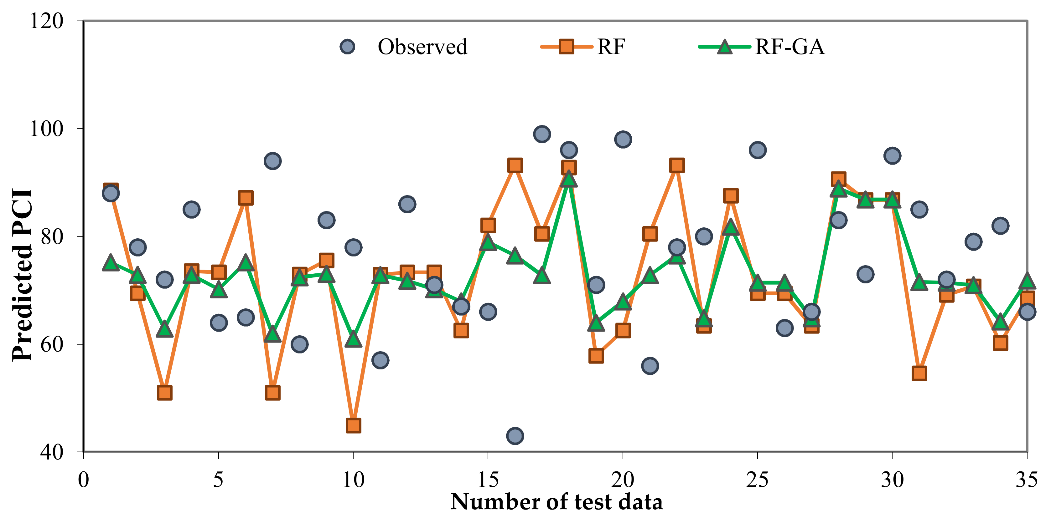
There has been no standard method for splitting training and testing data. For example, Nabipour et al. [37] utilized 70% of their data for training, whereas Mohammadzadeh et al. [87], Shamshirband et al. [88], and Samadarianfard et al. [89] applied 70%, 67%, and 80% of total data to develop their models. In this study, the dataset includes 118 pavement segments where approximately 70% of the data (i.e., 83 segments) are utilized for training, and the remaining 35 segments are used for testing. Figure 5 depicts the PCI predicted by the RF and RF-GA methods as well as the PCI calculated in the experimental phase of the study. As shown in Figure 5, the RF-GA method’s predictions are closer to the actual values than the RF method. Examination of the green and orange curves, as well as the blue circles (observed PCI), shows that the green curve (RF-GA method) has less error in the estimation of PCI than the orange curve (RF method). Therefore, it can be said that the RF-GA method is more successful than the RF method.

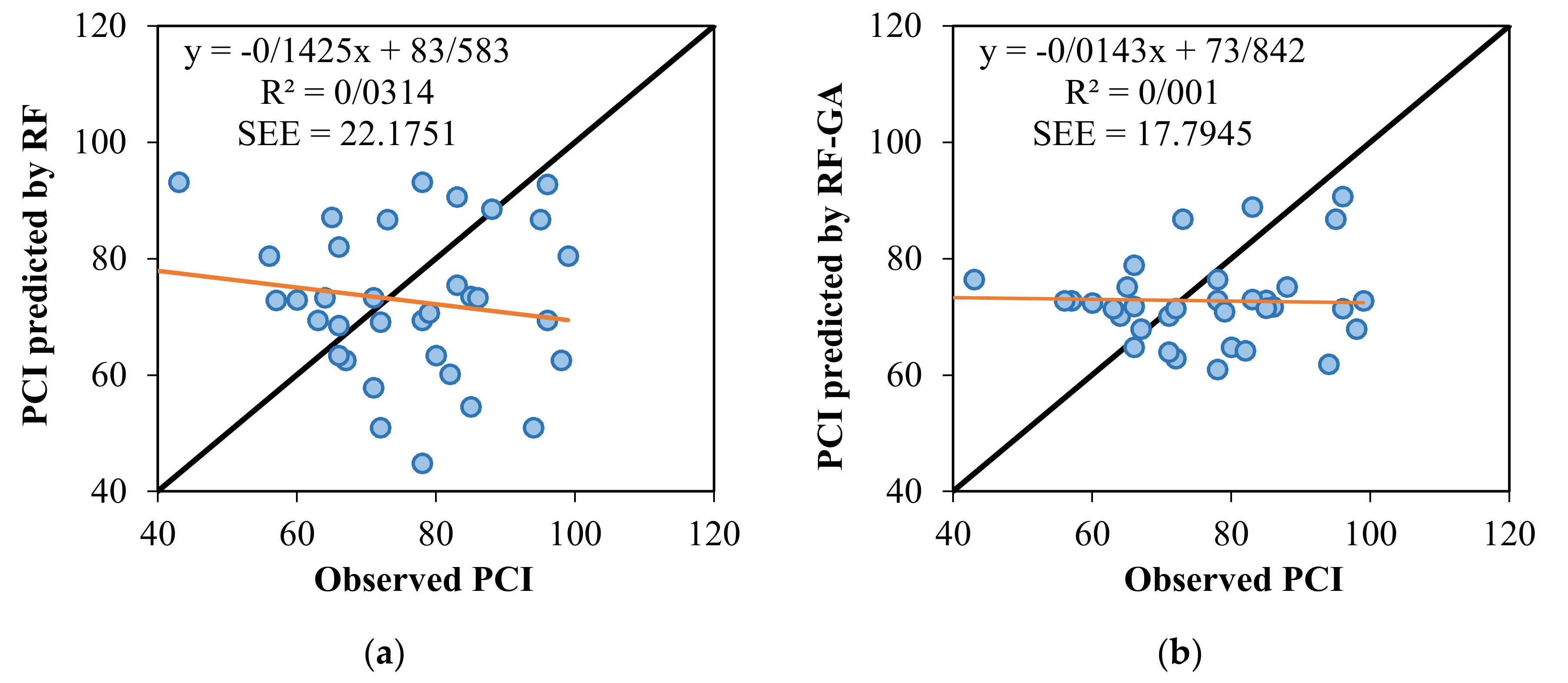
Figure 6 shows the calculated PCIs in the experimental phase of the study and predicted PCIs with RF and RF-GA models for test data. In this figure, three factors have been used to evaluate the accuracy of the results: trend line, r-square (R²), and standard error of the estimate (SEE). The trend line, or line of best fit, is a straight line that best represents the data on a scatter plot. The best trend line is y = x, a line with the slope of one and y-intercept of zero. When the y-intercept and slope of a trend line are closer to the values of zero and one, respectively, the results of that trend line are more accurate. R² is the square of the correlation coefficient between the observed and the predicted data. R² ranges from 0 to 1. The SEE is a measure of the accuracy of predictions made with a trend line. The trend line seeks to minimize the sum of the squared errors of prediction. SEE is closely related to this quantity and is defined in Equation (12). For any trend lines, a greater R² and lesser SEE mean more accurate results [37,90,91]. Based on Figure 6, GA can improve the y-intercept of the trend line in the RF model. Also, SEE is reduced by GA. However, regarding the slope and R² of the trend line, GA is not successful.

$$\mathrm{SEE}=\sqrt{\frac{1}{\mathrm{n}}{\displaystyle \sum }_{\mathrm{i}=1}^{\mathrm{n}}{\left({\mathrm{PCI}}_{\mathrm{Pi}}-{\mathrm{PCI}}_{\mathrm{Oi}}\right)}^2}$$

(12)

where PCI_Oi, PCI_Pi, and n are ith observed PCI, ith PCI predicted by the model, and the number of observed PCI values, respectively.

A review of other approaches reported in the background, except for a case [27], shows that other models’ correlation, check [18,25,26,28], is generally moderate. Also, the number of data used for modeling is very low in some cases. This can affect the reliability of the results. Many studies have used simple statistical techniques to analyze data. However, the present study’s authors have turned to two of the most powerful machine learning methods, namely the random forest and genetic algorithm. On the other hand, the data used in this study are related to one of the most important and busiest freeways in Iran, Tehran-Qom freeway. The data covers the entire route of this freeway. Therefore, the data in this paper can be considered qualitatively and quantitatively acceptable. To conduct this research, the authors faced several limitations. One of the most important constraints faced by these authors was interference with the traffic flow. This limited the number of sample units under review. The authors were very interested in using other non-destructive equipment such as falling weight deflectometer (FWD) or ground penetrating radar (GPR). Restrictions on blocking the freeway, as well as financial constraints, prevented the study’s authors from using the equipment. The authors believed that, by adding new parameters, such as road class, weather indicators, traffic compositions, the thickness of pavement layers, or the structural evaluation results, such as SN, etc., more accurate and reliable results can be achieved. Unfortunately, the Iranian Ministry of Roads and Urban Development restrictions did not allow the authors to use these parameters.

5. Conclusions

The present research explores the potential of machine learning techniques for overcoming the challenges of traditional methods for pavement assessment. Regarding the importance of the constant evaluation of the surface condition and the roughness in the pavement network, the authors have focused on two main indices, namely PCI and IRI. The authors examined the relationship between these two parameters using machine learning methods to determine the best methods for PCI estimation.

• Machine learning methods have shown promising results in managing the field equipment availability and further improving the pavement management system’s efficiency.
• Among the methods used in this study, the best results were obtained for RF and RF-GA.
• The proposed approach allows pavement engineers to calculate IRI and PCI simultaneously with only the input of RSP and ML methods.
• The proposed methodology can be further improved using a sophisticated machine learning approach with higher performance. Training novel machine learning methods with various evolutionary algorithms and using hybrid and ensemble methods would lead to higher accuracy models.

In future studies, novel models can be tested in various scenarios to evaluate and improve the feasibility. Increasing the number of sections under study, inserting new variables in modeling, e.g., traffic patterns, layers characteristics, and cracking features, and employing other non-destructive types of equipment, e.g., GPR and FWD, would be essential in developing the new scenarios. Using such novel models, we can substantially reduce the cost and time.

References

1. Patrick, G.; Soliman, H. Roughness prediction models using pavement surface distresses in different Canadian climatic regions. Can. J. Civ. Eng. 2019, 46, 934–940. [Google Scholar] [CrossRef]
2. Kulkarni, R.B.; Miller, R.W. Pavement management systems: Past, present, and future. Transp. Res. Rec. 2003, 1853, 65–71. [Google Scholar] [CrossRef]
3. Moghadas Nejad, F. Pavement Management System Framework in Iran; Transportation Research Institute (TRI): Tehran, Iran, 2009; p. 398. [Google Scholar]
4. Jahanshahi, M.R.; Karimi, F.J.; Masri, S.F.; Becerik-Gerber, B. Autonomous Pavement Condition Assessment. U.S. Patent 9,196,048, 24 November 2015. [Google Scholar]
5. Abdelaziz, N.; Abd El-Hakim, R.T.; El-Badawy, S.M.; Afify, H.A. International roughness index prediction model for flexible pavements. Int. J. Pavement Eng. 2020, 21, 88–99. [Google Scholar] [CrossRef]
6. Abudinen, D.; Fuentes, L.G.; Carvajal Muñoz, J.S. Travel quality assessment of urban roads based on international roughness index: Case study in Colombia. Transp. Res. Rec. 2017, 2612, 1–10. [Google Scholar] [CrossRef]
7. Walubita, L.F.; Scullion, T. Perpetual Pavements in Texas: The Fort Worth SH 114 Project in Wise County; Texas Transportation Institute: San Antonio, TX, USA, 2007. [Google Scholar]
8. Fuentes, L.; Camargo, R.; Martínez-Arguelles, G.; Komba, J.J.; Naik, B.; Walubita, L.F. Pavement serviceability evaluation using whole body vibration techniques: A case study for urban roads. Int. J. Pavement Eng. 2019, 1–12. [Google Scholar] [CrossRef]
9. Firoozi Yeganeh, S.; Mahmoudzadeh, A.; Azizpour, M.A.; Golroo, A. Validation of smartphone-based pavement roughness measures. Civil Eng. 2019, 1, 135–144. [Google Scholar]
10. Semnarshad, M.; Elyasi, M.; Saffarzadeh, M.; Saffarzadeh, A. Identification and Prioritization of Accident-Prone Segments using International Roughness Index. Int. J. Transp. Eng. 2018, 6, 35–48. [Google Scholar]
11. Shahin, M.Y. Pavement Management for Airports, Roads, and Parking Lots; Springer: New York, NY, USA, 2005; Volume 501. [Google Scholar]
12. Majidifard, H.; Adu-Gyamfi, Y.; Buttlar, W.G. Deep machine learning approach to develop a new asphalt pavement condition index. Constr. Build. Mater. 2020, 247, 118513. [Google Scholar] [CrossRef]
13. Janoff, M.S.; Nick, J.; Davit, P.; Hayhoe, G.F. Pavement roughness and rideability. In NCHRP Reports; Transportation Research Board: Washington, DC, USA, 1985. [Google Scholar]
14. Mubaraki, M. Highway subsurface assessment using pavement surface distress and roughness data. Int. J. Pavement Res. Technol. 2016, 9, 393–402. [Google Scholar] [CrossRef] [Green Version]
15. Chandra, S.; Sekhar, C.R.; Bharti, A.K.; Kangadurai, B. Relationship between pavement roughness and distress parameters for Indian highways. J. Transp. Eng. 2013, 139, 467–475. [Google Scholar] [CrossRef]
16. Mactutis, J.A.; Alavi, S.H.; Ott, W.C. Investigation of relationship between roughness and pavement surface distress based on WesTrack project. Transp. Res. Rec. 2000, 1699, 107–113. [Google Scholar] [CrossRef]
17. Lin, J.-D.; Yau, J.-T.; Hsiao, L.-H. Correlation analysis between international roughness index (IRI) and pavement distress by neural network. In Proceedings of the 82nd Annual Meeting of the Transportation Research Board, Washington, DC, USA, 12–16 January 2003; pp. 12–16. [Google Scholar]
18. Park, K.; Thomas, N.E.; Wayne Lee, K. Applicability of the international roughness index as a predictor of asphalt pavement condition. J. Transp. Eng. 2007, 133, 706–709. [Google Scholar] [CrossRef]
19. Taghavi Ghalesari, A.; Aguirre, N.; Carrasco, C.J.; Vrtis, M.; Garg, N. Evaluation of the response from the rigid pavement analysis system (RPAS) program for the characterisation of jointed concrete pavements. Road Mater. Pavement Des. 2020, 1–20. [Google Scholar] [CrossRef]
20. Von Quintus, H.L.; Eltahan, A.; Yau, A. Smoothness models for hot-mix asphalt-surfaced pavements: Developed from long-term pavement performance program data. Transp. Res. Rec. 2001, 1764, 139–156. [Google Scholar] [CrossRef]
21. Kargah-Ostadi, N. Comparison of machine learning techniques for developing performance prediction models. In 2014 International Conference on Computing in Civil and Building Engineering; American Society of Civil Engineers: Orlando, FL, USA, 17 June 2014; pp. 1222–1229. [Google Scholar]
22. Sharaf, E.A.; Hanno, D.F. An Analysis of the Effect of Pavement Condition on Vehicle Operating Costs. In Proceedings of the Al-Azhar Engineering First Conference, Cairo, Egypt, 12–14 December 2017. [Google Scholar]
23. Abd-Allah, A. Analysis of flexible pavement roughness in egypt. Master’s Thesis, Zagazig University, Zagazig, Egypt, 1990. [Google Scholar]
24. Sharaf, A.; Mandeel, F.M. An analysis of the impact of different priority setting techniques on network pavement condition. In Proceedings of the 4th International Conference on Managing Pavements, Durban, South Africa, 17–21 May 1998; pp. 158–168. [Google Scholar]
25. Shameem, A.; Dewan, R.E.S. Estimating international roughness index from pavement distresses to calculate vehicle operating costs for the san francisco bay area. Transp. Res. Rec. 2002, 1816, 65–72. [Google Scholar] [CrossRef]
26. Arhin, S.A.; Williams, L.N.; Ribbiso, A.; Anderson, M.F. Predicting pavement condition index using international roughness index in a dense urban area. J. Civ. Eng. Res. 2015, 5, 10–17. [Google Scholar]
27. Elhadidy, A.A.; El-Badawy, S.M.; Elbeltagi, E.E. A simplified pavement condition index regression model for pavement evaluation. Int. J. Pavement Eng. 2019, 1–10. [Google Scholar] [CrossRef]
28. Ali, A.; Hossain, K.; Hussein, A.; Swarna, S.; Dhasmana, H.; Hossain, M. Towards development of PCI and IRI models for road networks in the City of St. John’s. In Airfield and Highway Pavements 2019: Design, Construction, Condition Evaluation, and Management of Pavements; American Society of Civil Engineers: Reston, VA, USA, 2019; pp. 335–342. [Google Scholar]
29. Marcelino, P.; Lurdes Antunes, M.d.; Fortunato, E.; Castilho Gomes, M. Machine learning approach for pavement performance prediction. Int. J. Pavement Eng. 2019, 1–14. [Google Scholar] [CrossRef]
30. Hoang, N.-D.; Nguyen, Q.-L. A novel method for asphalt pavement crack classification based on image processing and machine learning. Eng. Comput. 2019, 35, 487–498. [Google Scholar] [CrossRef]
31. Hoang, N.-D.; Nguyen, Q.-L. Automatic recognition of asphalt pavement cracks based on image processing and machine learning approaches: A comparative study on classifier performance. Math. Probl. Eng. 2018, 2018, 6290498. [Google Scholar] [CrossRef]
32. Hoang, N.-D.; Nguyen, Q.-L.; Tien Bui, D. Image processing-based classification of asphalt pavement cracks using support vector machine optimized by artificial bee colony. J. Comput. Civ. Eng. 2018, 32, 04018037. [Google Scholar] [CrossRef]
33. Moghadas Nejad, F.; Mehrabi, A.; Zakeri, H. Prediction of asphalt mixture resistance using neural network via laboratorial X-ray images’. J. Ind. Intell. Inf. Vol 2015, 3. [Google Scholar] [CrossRef]
34. Moghadas Nejad, F.; Zare Motekhases, F.; Zakeri, H.; Mehrabi, A. An image processing approach to asphalt concrete feature extraction. J. Ind. Intell. Inf. Vol 2015, 3. [Google Scholar] [CrossRef]
35. Fathi, A.; Mazari, M.; Saghafi, M.; Hosseini, A.; Kumar, S. Parametric study of pavement deterioration using machine learning algorithms. In Airfield and Highway Pavements 2019: Innovation and Sustainability in Highway and Airfield Pavement Technology; American Society of Civil Engineers: Reston, VA, USA, 2019; pp. 31–41. [Google Scholar]
36. Souza, V.M.; Giusti, R.; Batista, A.J. Asfault: A low-cost system to evaluate pavement conditions in real-time using smartphones and machine learning. Pervasive Mob. Comput. 2018, 51, 121–137. [Google Scholar] [CrossRef]
37. Nabipour, N.; Karballaeezadeh, N.; Dineva, A.; Mosavi, A.; Mohammadzadeh, S.D.; Shamshirband, S. Comparative analysis of machine learning models for prediction of remaining service life of flexible pavement. Mathematics 2019, 7, 1198. [Google Scholar] [CrossRef] [Green Version]
38. Fujita, Y.; Shimada, K.; Ichihara, M.; Hamamoto, Y. A method based on machine learning using hand-crafted features for crack detection from asphalt pavement surface images. In Proceedings of the Thirteenth International Conference on Quality Control by Artificial Vision 2017, Tokyo, Japan, 14–16 May 2017; p. 103380I. [Google Scholar]
39. Nitsche, P.; Stütz, R.; Kammer, M.; Maurer, P. Comparison of machine learning methods for evaluating pavement roughness based on vehicle response. J. Comput. Civ. Eng. 2014, 28, 04014015. [Google Scholar] [CrossRef]
40. Karballaeezadeh, N.; Mohammadzadeh, S.D.; Shamshirband, S.; Hajikhodaverdikhan, P.; Mosavi, A.; Chau, K.-W. Prediction of remaining service life of pavement using an optimized support vector machine (case study of Semnan–Firuzkuh road). Eng. Appl. Comput. Fluid Mech. 2019, 13, 188–198. [Google Scholar] [CrossRef] [Green Version]
41. Karballaeezadeh, N.; Tehrani, H.G.; Mohammadzadeh, D.; Shamshirband, S. Estimation of flexible pavement structural capacity using machine learning techniques. Front. Struct. Civ. Eng. 2020, 14. [Google Scholar] [CrossRef]
42. Inkoom, S.; Sobanjo, J.; Barbu, A.; Niu, X. Pavement crack rating using machine learning frameworks: Partitioning, bootstrap forest, boosted trees, Naïve bayes, and K-Nearest neighbors. J. Transp. Eng. Part B Pavements 2019, 145, 04019031. [Google Scholar] [CrossRef]
43. Zeiada, W.; Dabous, S.A.; Hamad, K.; Al-Ruzouq, R.; Khalil, M.A. Machine learning for pavement performance modelling in warm climate regions. Arab. J. Sci. Eng. 2020, 45, 4091–4109. [Google Scholar] [CrossRef]
44. Cao, R.; Leng, Z.; Hsu, S.-C.; Hung, W.-T. Modelling of the pavement acoustic longevity in Hong Kong through machine learning techniques. Transp. Res. Part D Transp. Environ. 2020, 83, 102366. [Google Scholar] [CrossRef]
45. Miller, J.S.; Bellinger, W.Y. Distress Identification Manual for the Long-Term Pavement Performance Program; Office of Infrastructure, Federal Highway Administration: McLean, VA, USA, 2003. [Google Scholar]
46. Gharaibeh, N.G.; Zou, Y.; Saliminejad, S. Assessing the agreement among pavement condition indexes. J. Transp. Eng. 2009, 136, 765–772. [Google Scholar] [CrossRef]
47. Karballaeezadeh, N.; Zaremotekhases, F.; Shamshirband, S.; Mosavi, A.; Nabipour, N.; Csiba, P.; Várkonyi-Kóczy, A.R. Intelligent Road Inspection with Advanced Machine Learning; Hybrid Prediction Models for Smart Mobility and Transportation Maintenance Systems. Energies 2020, 13, 1718. [Google Scholar] [CrossRef] [Green Version]
48. ASTM D6433-18, Standard Practice for Roads and Parking Lots Pavement Condition Index Surveys; ASTM International: West Conshohocken, PA, USA, 2018; Available online: www.astm.org (accessed on 25 May 2018).
49. Múčka, P. International Roughness Index specifications around the world. Road Mater. Pavement Des. 2017, 18, 929–965. [Google Scholar] [CrossRef]
50. Hudson, W.R.; Haas, R.; Pedigo, R.D. Pavement management system development. In NCHRP Report 215; Transportation Research Board: Washington, DC, USA, 1979. [Google Scholar]
51. Szénási, S.; Kertész, G.; Felde, I.; Nádai, L. Statistical accident analysis supporting the control of autonomous vehicles. J. Comput. Methods Sci. Eng. 2020, 1–13. [Google Scholar] [CrossRef]
52. Ullidtz, P. Pavement Analysis. Developments in Civil Engineering, 19; North Holland: Amsterdam, Netherlands, 1987. [Google Scholar]
53. Yu, J.; Chou, E.Y.; Yau, J.-T. Development of speed-related ride quality thresholds using international roughness index. Transp. Res. Rec. 2006, 1974, 47–53. [Google Scholar] [CrossRef]
54. Mazari, M.; Rodriguez, D.D. Prediction of pavement roughness using a hybrid gene expression programming-neural network technique. J. Traffic Transp. Eng. Engl. Ed. 2016, 3, 448–455. [Google Scholar] [CrossRef] [Green Version]
55. Bilodeau, J.-P.; Gagnon, L.; Doré, G. Assessment of the relationship between the international roughness index and dynamic loading of heavy vehicles. Int. J. Pavement Eng. 2017, 18, 693–701. [Google Scholar] [CrossRef]
56. Sayers, M.W. On the calculation of international roughness index from longitudinal road profile. Transp. Res. Rec. 1995, 1501, 1–12. [Google Scholar]
57. Zoccali, P.; Loprencipe, G.; Galoni, A. Sampietrini stone pavements: Distress analysis using pavement condition index method. Appl. Sci. 2017, 7, 669. [Google Scholar] [CrossRef] [Green Version]
58. Ozbay, K.; Laub, R. Models for Pavement Deterioration Using LTPP; Federal Highway Administration (FHWA): Washington, DC, USA, 2001. [Google Scholar]
59. Status of the Nation’s Highways, Bridges, and Transit: Conditions and Performance; Federal HighWay Administration (FHWA): Washington, DC, USA, 1999.
60. Yang, S.; Ceylan, H.; Gopalakrishnan, K.; Kim, S.; Taylor, P.C.; Alhasan, A. Characterization of environmental loads related concrete pavement deflection behavior using Light Detection and Ranging technology. Int. J. Pavement Res. Technol. 2018, 11, 470–480. [Google Scholar] [CrossRef]
61. Bosché, F.; Guenet, E. Automating surface flatness control using terrestrial laser scanning and building information models. Autom. Constr. 2014, 44, 212–226. [Google Scholar] [CrossRef]
62. Wang, Q.; Kim, M.-K.; Sohn, H.; Cheng, J.C. Surface flatness and distortion inspection of precast concrete elements using laser scanning technology. Smart Struct. Syst. 2016, 18, 601–623. [Google Scholar] [CrossRef] [Green Version]
63. Gong, H.; Sun, Y.; Shu, X.; Huang, B. Use of random forests regression for predicting IRI of asphalt pavements. Constr. Build. Mater. 2018, 189, 890–897. [Google Scholar] [CrossRef]
64. Li, Z.; Cheng, C.; Kwan, M.-P.; Tong, X.; Tian, S. Identifying asphalt pavement distress using UAV LiDAR point cloud data and random forest classification. ISPRS Int. J. Geo-Inf. 2019, 8, 39, reprinted in ISPRS Int. J. Geo-Inf. 2019, 9, 402. [Google Scholar] [CrossRef] [Green Version]
65. Breiman, L.; Friedman, J.; Olshen, R.; Stone, C. Classification and regression trees. Wadsworth Int. Group 1984, 37, 237–251. [Google Scholar]
66. Sadler, J.; Goodall, J.; Morsy, M.; Spencer, K. Modeling urban coastal flood severity from crowd-sourced flood reports using poisson regression and random forest. J. Hydrol. 2018, 559, 43–55. [Google Scholar] [CrossRef]
67. Yang, G.; Yu, W.; Li, Q.J.; Wang, K.; Peng, Y.; Zhang, A. Random forest–based pavement surface friction prediction using high-resolution 3D image data. J. Test. Eval. 2019, 49. [Google Scholar] [CrossRef]
68. Shabani, S.; Samadianfard, S.; Sattari, M.T.; Mosavi, A.; Shamshirband, S.; Kmet, T.; Várkonyi-Kóczy, A.R. Modeling pan evaporation using gaussian process regression k-nearest neighbors random forest and support vector machines; Comparative analysis. Atmosphere 2020, 11, 66. [Google Scholar] [CrossRef] [Green Version]
69. Zhang, S.; Tan, Z.; Liu, J.; Xu, Z.; Du, Z. Determination of the food dye indigotine in cream by near-infrared spectroscopy technology combined with random forest model. Spectrochim. Acta Part A Mol. Biomol. Spectrosc. 2020, 227, 117551. [Google Scholar] [CrossRef]
70. Elyan, E.; Gaber, M.M. A genetic algorithm approach to optimising random forests applied to class engineered data. Inf. Sci. 2017, 384, 220–234. [Google Scholar] [CrossRef]
71. Prasad, A.M.; Iverson, L.R.; Liaw, A. Newer classification and regression tree techniques: Bagging and random forests for ecological prediction. Ecosystems 2006, 9, 181–199. [Google Scholar] [CrossRef]
72. Breiman, L. Random forests. Mach. Learn. 2001, 45, 5–32. [Google Scholar] [CrossRef] [Green Version]
73. Sun, H.; Gui, D.; Yan, B.; Liu, Y.; Liao, W.; Zhu, Y.; Lu, C.; Zhao, N. Assessing the potential of random forest method for estimating solar radiation using air pollution index. Energy Convers. Manag. 2016, 119, 121–129. [Google Scholar] [CrossRef] [Green Version]
74. Singh, T.; Pal, M.; Arora, V. Modeling oblique load carrying capacity of batter pile groups using neural network, random forest regression and M5 model tree. Front. Struct. Civ. Eng. 2019, 13, 674–685. [Google Scholar] [CrossRef]
75. Mutanga, O.; Adam, E.; Cho, M.A. High density biomass estimation for wetland vegetation using WorldView-2 imagery and random forest regression algorithm. Int. J. Appl. Earth Obs. Geoinf. 2012, 18, 399–406. [Google Scholar] [CrossRef]
76. Douglas, R.K.; Nawar, S.; Alamar, M.C.; Mouazen, A.; Coulon, F. Rapid prediction of total petroleum hydrocarbons concentration in contaminated soil using vis-NIR spectroscopy and regression techniques. Sci. Total Environ. 2018, 616, 147–155. [Google Scholar] [CrossRef] [Green Version]
77. Nawar, S.; Mouazen, A.M. Comparison between random forests, artificial neural networks and gradient boosted machines methods of on-line Vis-NIR spectroscopy measurements of soil total nitrogen and total carbon. Sensors 2017, 17, 2428. [Google Scholar] [CrossRef]
78. Horton, P.; Jaboyedoff, M.; Obled, C. Using genetic algorithms to optimize the analogue method for precipitation prediction in the Swiss Alps. J. Hydrol. 2018, 556, 1220–1231. [Google Scholar] [CrossRef] [Green Version]
79. Sindi, W.; Agbelie, B. Assignments of pavement treatment options: Genetic algorithms versus mixed-integer programming. J. Transp. Eng. Part B Pavements 2020, 146, 04020008. [Google Scholar] [CrossRef]
80. Santos, J.; Ferreira, A.; Flintsch, G. An adaptive hybrid genetic algorithm for pavement management. Int. J. Pavement Eng. 2019, 20, 266–286. [Google Scholar] [CrossRef]
81. Preis, A.; Ostfeld, A. A coupled model tree–genetic algorithm scheme for flow and water quality predictions in watersheds. J. Hydrol. 2008, 349, 364–375. [Google Scholar] [CrossRef]
82. Sebaaly, H.; Varma, S.; Maina, J.W. Optimizing asphalt mix design process using artificial neural network and genetic algorithm. Constr. Build. Mater. 2018, 168, 660–670. [Google Scholar] [CrossRef] [Green Version]
83. Davis, L. Handbook of Genetic Algorithms; Van Nostrand Reinhold: New York, NY, USA, 1991. [Google Scholar]
84. Alam, M.N.; Das, B.; Pant, V. A comparative study of metaheuristic optimization approaches for directional overcurrent relays coordination. Electr. Power Syst. Res. 2015, 128, 39–52. [Google Scholar] [CrossRef]
85. Mendenhall, W.M.; Sincich, T.L. Statistics for Engineering and the Sciences; CRC Press: Boca Raton, FL, USA, 2016. [Google Scholar]
86. George, D.; Mallery, P. IBM SPSS Statistics 23 Step by Step: A Simple Guide and Reference; Routledge: Abingdon, UK, 2016. [Google Scholar]
87. Mohammadzadeh, S.; Kazemi, S.-F.; Mosavi, A.; Nasseralshariati, E.; Tah, J.H. Prediction of compression index of fine-grained soils using a gene expression programming model. Infrastructures 2019, 4, 26. [Google Scholar] [CrossRef] [Green Version]
88. Shamshirband, S.; Hadipoor, M.; Baghban, A.; Mosavi, A.; Bukor, J.; Várkonyi-Kóczy, A.R. Developing an ANFIS-PSO model to predict mercury emissions in combustion flue gases. Mathematics 2019, 7, 965. [Google Scholar] [CrossRef] [Green Version]
89. Samadianfard, S.; Jarhan, S.; Salwana, E.; Mosavi, A.; Shamshirband, S.; Akib, S. Support vector regression integrated with fruit fly optimization algorithm for river flow forecasting in lake urmia basin. Water 2019, 11, 1934. [Google Scholar] [CrossRef] [Green Version]
90. Siegel, A. Practical Business Statistics; Academic Press: Cambridge, MA, USA, 2016. [Google Scholar]
91. Isa, A.; Ma’Soem, D.; Hwa, L.T. Pavement performance model for federal roads. In Proceedings of the Eastern Asia Society for Transportation Studies, Bangkok, Thailand, 21–24 September 2005; pp. 428–440. [Google Scholar]
Figure 1. The quarter-car system in the IRI calculation process.
Coatings 10 01100 g001
Figure 2. The RSP device used in this research.
Coatings 10 01100 g002
Figure 3. The line laser system for determining IRI in wheels paths.
Coatings 10 01100 g003
Figure 4. The random forest process.
Coatings 10 01100 g004
Figure 5. Observed and predicted values of PCI with RF and RF-GA models.
Coatings 10 01100 g005
Figure 6. The scatter plots of calculated PCI in the experimental phase of the study and predicted PCI with RF and RF-GA models for test data. (a) RF; (b) RF-GA.
Coatings 10 01100 g006