Modeling of Imperfect Viscoelastic Interfaces in Composite Materials

Abstract

The present work deals with hierarchical composites in three dimensions, whose constituents behave as non-aging linear viscoelastic materials. We model the influence that imperfect viscoelastic interfaces have on the macroscopic effective response of these structures. As an initial approach, the problem of two bodies in adhesion is studied and in particular the case of soft viscoelastic interface at zero-order is considered. We deduce the integral form of the viscoelastic interface by applying the matched asymptotic expansion method, the correspondence principle, and the Laplace–Carson transform. Then, by adapting the integral form previously obtained, we address a heterogeneous problem for periodic structures. Here, theoretical results obtained for perfect interfaces are extended to the formal viscoelastic counterpart of the spring-type imperfect interface model. Finally, we show the potential of the proposed approach by performing calculations of effective properties in heterogeneous structures with two- and three-scale geometrical configurations and imperfect viscoelastic interfaces.

1. Introduction

The modeling of imperfect interfaces in composite materials plays an essential role in mechanical and civil engineering applications. The physical phenomena commonly studied are, for instance, adhesion, non-conforming contact, microcracks, friction, unilateral contact, among others. It is worth mentioning that conventional adhesives such as water-based polymers generally exhibit viscoelastic properties (see [1,2]), hence the importance of studying the viscoelastic response in imperfect interfaces models. In this regard, recent studies address the influence of viscoelastic imperfect interfaces in composite materials (see, e.g., [3,4,5,6,7]).

Several interface models based on micromechanical approaches have been proposed. One of the first definitions of imperfect interfaces is certainly to be found in the works of [8,9,10,11]. In particular, in [9], the author defines the imperfect interface in terms of the spring-type model, relating the displacement jumps at the interface to tractions. In addition, the author assumes that the discontinuity in terms of displacements is allowed and linearly proportional to the traction vector; however, the continuity in terms of stresses, according to local equilibrium, is preserved (see [12] for more details). This approach, adapted to the homogenization of composites materials with periodic microstructure, has been widely used in recent contributions (see, e.g., [13,14,15,16]).

Another treatment for bonded regions has been recently proposed by [17]. In this regard, the authors model the asymptotic behavior of a thin interphase at higher orders for two cases, i.e., soft and hard interface materials, by means of a unified approach. Specifically, the adhesive is replaced by an elastic interface that retains in the memory the main mechanical characteristics of this material (see [18]). A classical theory for obtaining this material interface is the method of matched asymptotic expansions (see [19]). It is worth noticing that, when considering up to zero order of the asymptotic expansion, if the adhesive is soft, then the proposed approach covers the models based on the classical law of the spring-type interface, and additionally, if the adhesive is hard, it returns the classical model of perfect interface, where both the traction and displacement vector fields are continuous across the interface. This methodology has been addressed in several contributions, see, e.g., [20,21,22,23,24,25].

In the present work, the influence that imperfect viscoelastic interfaces have on the macroscopic effective response of heterogeneous structures is studied. Several studies have been carried out to model thin layers and interfaces using viscoelastic models such as Maxwell and Kelvin–Voigt (see, e.g., [26]). In this regard, the main novelty of the work lies in considering the integral representation of the imperfect viscoelastic interface for displacement-type discontinuity conditions. Moreover, this imperfect viscoelastic interface is integrated into the model addressed in [27], which is devoted to hierarchical viscoelastic composites.

In summary, the work is divided into two stages. In the first stage, the viscoelastic law of the imperfect interface is derived by studying the two-body bonding problem via matched asymptotic expansions (see [19]), where the adhesive and some of the adherents behave as linear viscoelastic materials (refer to Section 2). In the second stage, a problem for hierarchical heterogeneous structures with non-aging linear viscoelastic constituents and imperfect contact conditions is modeled by means of the three-scale Asymptotic Homogenization Method (AHM) (see Section 3). Additionally, in Section 4, a methodology is presented to solve analytically the local problem in the case of laminated composites with imperfect interfaces. Finally, in Section 5 and Section 6, we show the potential of the proposed approach by performing several calculations in the case of two- and three-scale configurations of heterogeneous structures with imperfect viscoelastic interfaces.

2. The Problem of Two Bodies in Adhesion

In this section, an assembly of two bodies is considered where the adhesive layer, also called interphase, is characterized by a low thickness. Because of this, it becomes problematic to address the heterogeneous problem by means of a finite element analysis. Therefore, the introduction of a scaling parameter and the use of asymptotic techniques arise as a suitable alternative for the solution of the problem (see, e.g., [28,29]). In general, the methodology consists of replacing the problem of the thin adhesive by a homogeneous problem wherein the small parameter is geometrically vanished in the limit theory and the mechanical properties of the new imperfect interfaces are derived from the mechanical and geometrical behavior of the original interphase (see more details in [12]). We recall that the purpose of this section is to generalize the theoretical framework developed in [17] by considering that the adhesive and some of the adherents behave as linear viscoelastic materials. In this regard, initial ideas for modeling thin layers and interfaces in viscoelastic Maxwell and Kelvin–Voigt models are reported in [26].

2.1. Model Description

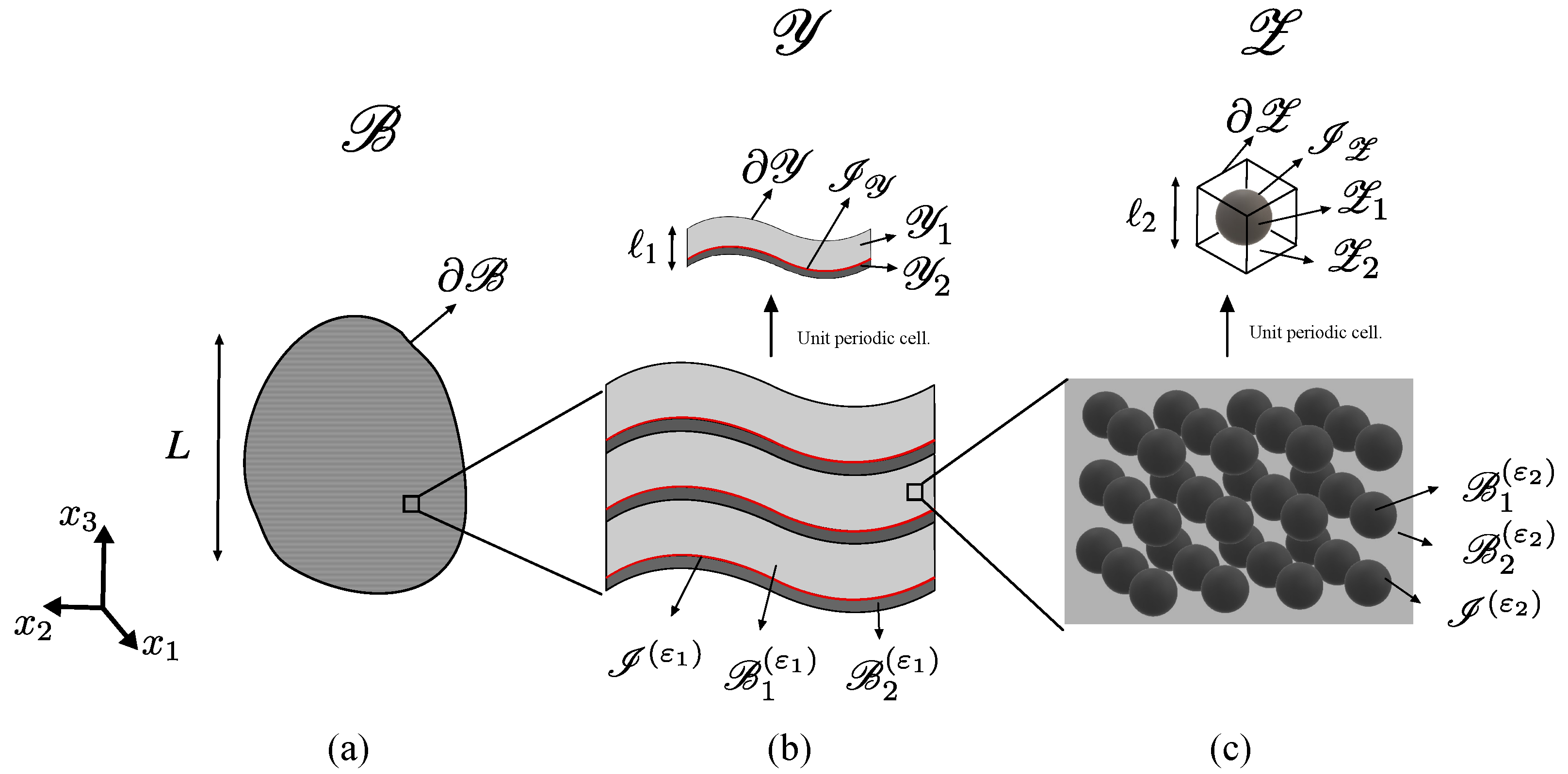
Let us consider a composite body ${\mathcal{B}}^{\left(h\right)}\subset {\mathbb{R}}^3$ made by three deformable and homogeneous solids, bonded together, and that behave as non-aging linear viscoelastic materials (see Figure 1a). In particular, two adherents denoted by ${\mathcal{B}}_{+}^{\left(h\right)}$ and ${\mathcal{B}}_{-}^{\left(h\right)}$ are joined by an adhesive (thin layer) ${\mathcal{D}}^{\left(h\right)}$ with uniform small thickness $h\ll 1$. The cross-section of ${\mathcal{D}}^{\left(h\right)}$ is referred to as $\mathcal{I}$, and represents an open bounded set in ${\mathbb{R}}^2$ with a smooth boundary $\partial \mathcal{I}$. Thus, ${\mathcal{D}}^{\left(h\right)}$ and $\mathcal{I}$ are known as interphase and interface, respectively. Additionally, ${\mathcal{I}}_{\pm }^{\left(h\right)}$ stands for the plane interfaces between the interphase and the adherents. The above leads to ${\mathcal{B}}^{\left(h\right)}={\mathcal{B}}_{\pm }^{\left(h\right)}\cup {\mathcal{I}}_{\pm }^{\left(h\right)}\cup {\mathcal{D}}^{\left(h\right)}$, whose domains and surfaces can be defined as follows:

$$\begin{array}{cc}\hfill & {\mathcal{B}}_{\pm }^{\left(h\right)}=\left\{(x_1,x_2,x_3)\in {\mathcal{B}}^{\left(h\right)}:\pm x_3>\frac{h}{2}\right\},\hfill \end{array}$$

(1)

$$\begin{array}{cc}\hfill & {\mathcal{D}}^{\left(h\right)}=\left\{(x_1,x_2,x_3)\in {\mathcal{B}}^{\left(h\right)}:-\frac{h}{2}<x_3<\frac{h}{2}\right\},\hfill \end{array}$$

(2)

$$\begin{array}{cc}\hfill & {\mathcal{I}}_{\pm }^{\left(h\right)}=\left\{(x_1,x_2,x_3)\in {\mathcal{B}}^{\left(h\right)}:x_3=\pm \frac{h}{2}\right\},\hfill \end{array}$$

(3)

$$\begin{array}{cc}\hfill & \mathcal{I}=\left\{(x_1,x_2,x_3)\in {\mathcal{B}}^{\left(h\right)}:x_3=0\right\}.\hfill \end{array}$$

(4)

Furthermore, the relaxation modulus for the adherents and the interphase are symmetric tensors, with the minor and major symmetries properties, and positive definite. They are denoted by ${\mathbb{B}}_{\pm }^{\left(h\right)}$ and ${\mathbb{D}}^{\left(h\right)}$, respectively.

The adherents are subjected to a body force density $\mathit{f}:{\mathcal{B}}_{\pm }^{\left(h\right)}\to {\mathbb{R}}^3$, which is negligible in the adhesive. In addition, a surface force density $\mathit{S}:\partial {\mathcal{B}}_n^{\left(h\right)}\to {\mathbb{R}}^3$ and homogeneous boundary conditions on $\partial {\mathcal{B}}_d^{\left(h\right)}$ are considered. It is worth mentioning that $\partial {\mathcal{B}}_n^{\left(h\right)}$ and $\partial {\mathcal{B}}_d^{\left(h\right)}$ are assumed to be located far from the interphase and the fields of the external forces are sufficiently regular to ensure the existence of an equilibrium configuration (see [17,21]).

Then, the equilibrium equation for the composite material reads

$$\begin{array}{cccc}\hfill & \nabla ·{\mathit{\sigma }}^{\left(h\right)}(x,t)+\mathit{f}(x,t)=\mathbf{0}\hfill & \hfill & \mathrm{in}{\mathcal{B}}_{\pm }^{\left(h\right)}\times \mathbb{R}\hfill \end{array}$$

(5)

$$\begin{array}{cccc}\hfill & \nabla ·{\mathit{\sigma }}^{\left(h\right)}(x,t)=\mathbf{0}\hfill & \hfill & \mathrm{in}{\mathcal{D}}^{\left(h\right)}\times \mathbb{R}\hfill \end{array}$$

(6)

$$\begin{array}{cccc}\hfill & {\mathit{u}}^{\left(h\right)}(x,t)=\mathbf{0}\hfill & \hfill & \mathrm{on}\partial {\mathcal{B}}_d^{\left(h\right)}\times \mathbb{R}\hfill \end{array}$$

(7)

$$\begin{array}{cccc}\hfill & {\mathit{\sigma }}^{\left(h\right)}(x,t)·\mathit{n}=\mathit{S}\hfill & \hfill & \mathrm{on}\partial {\mathcal{B}}_n^{\left(h\right)}\times \mathbb{R}\hfill \end{array}$$

(8)

$$\begin{array}{cccc}\hfill & ⟦{\mathit{u}}^{\left(h\right)}(x,t)⟧=\mathbf{0},⟦{\mathit{\sigma }}^{\left(h\right)}(x,t)·{\mathit{i}}_3⟧=\mathbf{0}\hfill & \hfill & \mathrm{on}{\mathcal{I}}_{\pm }^{\left(h\right)}\times \mathbb{R},\hfill \\ \hfill & \mathrm{Initial}\mathrm{condition}\mathrm{in}{\mathcal{B}}^{\left(h\right)}\times \left\{0\right\},\hfill \end{array}$$

(9)

$$\begin{array}{cc}\hfill & {\mathit{u}}^{\left(h\right)}(x,t)={\mathit{u}}_{\mathrm{e}}^{\left(h\right)}\left(x\right),\hfill \end{array}$$

(10)

where ($O,{\mathit{i}}_1,{\mathit{i}}_2,{\mathit{i}}_3$) is an orthonormal Cartesian basis.

As observed in (9), within the original interface problem, the adhesive ${\mathcal{D}}^{\left(h\right)}$ and the adherents ${\mathcal{B}}_{\pm }^{\left(h\right)}$ are assumed to be perfectly bonded and thus the continuity of the displacement and traction across ${\mathcal{I}}_{\pm }^{\left(h\right)}\times \mathbb{R}$ is guaranteed.

2.2. Matched Asymptotic Expansion Method

In this section, the main goal is to derive the viscoelastic imperfect interfaces from the viscoelastic behavior of the thin interphase. Since the thickness of the interphase is very small, it is natural to search for an approximate solution of problem (5)–(10) when the small parameter h vanishes (limit configuration). This is done by means of the matched asymptotic expansion method (see [17,19,30,31,32,33]). The approach relies on domain rescaling and employs series expansions of power of h for the rescaled fields. In what follows, the symbol ( $\stackrel{˘}{}$ ) represents the rescaled fields in the adhesive, whereas ( $\overline{}$ ) stands for the rescaled fields in the adherents.

2.2.1. Rescaling

The classical procedure starts with a change of variables in the adhesive and adherents, respectively (see [34]). In particular, at the adhesive, we have

$$\begin{array}{cc}\hfill & \breve{\mathit{p}}:(x_1,x_2,x_3)\in {\mathcal{D}}^{\left(h\right)}\mapsto (z_1,z_2,z_3)\in \mathcal{D}\hfill \end{array}$$

(11)

$$\begin{array}{cc}\hfill & z_1=x_1,z_2=x_2,z_3=\frac{x_3}{h},\hfill \end{array}$$

(12)

which gives

$$\begin{array}{cc}\hfill & \frac{\partial }{\partial z_1}=\frac{\partial }{\partial x_1},\frac{\partial }{\partial z_2}=\frac{\partial }{\partial x_2},\frac{\partial }{\partial z_3}=h\frac{\partial }{\partial x_3}.\hfill \end{array}$$

(13)

In addition, at the adherents is performed

$$\begin{array}{cc}\hfill & \overline{\mathit{p}}:(x_1,x_2,x_3)\in {\mathcal{B}}_{\pm }^{\left(h\right)}\mapsto (z_1,z_2,z_3)\in {\mathcal{B}}_{\pm }\hfill \end{array}$$

(14)

$$\begin{array}{cc}\hfill & z_1=x_1,z_2=x_2,z_3=x_3\pm \frac{1}{2}(1-h),\hfill \end{array}$$

(15)

where, similarly, the following is fulfilled:

$$\begin{array}{cc}\hfill & \frac{\partial }{\partial z_1}=\frac{\partial }{\partial x_1},\frac{\partial }{\partial z_2}=\frac{\partial }{\partial x_2},\frac{\partial }{\partial z_3}=\frac{\partial }{\partial x_3}.\hfill \end{array}$$

(16)

After these transformations, the structure shown in Figure 1b is reached, and geometrically we observe the following

$$\begin{array}{cc}\hfill & {\mathcal{B}}_{\pm }=\left\{(z_1,z_2,z_3)\in {\mathbb{R}}^3:\pm z_3>\frac{1}{2}\right\},\hfill \end{array}$$

(17)

$$\begin{array}{cc}\hfill & \mathcal{D}=\left\{(z_1,z_2,z_3)\in {\mathbb{R}}^3:-\frac{1}{2}<z_3<\frac{1}{2}\right\},\hfill \end{array}$$

(18)

$$\begin{array}{cc}\hfill & {\mathcal{I}}_{\pm }=\left\{(z_1,z_2,z_3)\in {\mathbb{R}}^3:z_3=\pm \frac{1}{2}\right\}.\hfill \end{array}$$

(19)

Moreover, the physical quantities involved in the problem (5)–(10) satisfy the corresponding transformation for all $t\in \mathbb{R}$, namely

$$\begin{array}{cc}\hfill & {\overline{\mathit{\sigma }}}^{\left(h\right)}:={\mathit{\sigma }}^{\left(h\right)}\circ {\overline{\mathit{p}}}^{-1},{\breve{\mathit{\sigma }}}^{\left(h\right)}:={\mathit{\sigma }}^{\left(h\right)}\circ {\breve{\mathit{p}}}^{-1}.\hfill \end{array}$$

(20)

$$\begin{array}{cc}\hfill & {\overline{\mathit{u}}}^{\left(h\right)}:={\mathit{u}}^{\left(h\right)}\circ {\overline{\mathit{p}}}^{-1},{\breve{\mathit{u}}}^{\left(h\right)}:={\mathit{u}}^{\left(h\right)}\circ {\breve{\mathit{p}}}^{-1}.\hfill \end{array}$$

(21)

$$\begin{array}{cc}\hfill & \overline{\mathit{f}}:=\mathit{f}\circ {\overline{\mathit{p}}}^{-1},\overline{\mathit{S}}:=\mathit{S}\circ {\overline{\mathit{p}}}^{-1},\hfill \end{array}$$

(22)

where, in Equations (20) and (21), the stress and displacement fields from the rescaled adhesive and adherents are respectively presented, whereas, in Equation (22), we have the rescaled external forces. Notice that the symbol “∘” in (20)–(22) denotes the function composition operator.

2.2.2. Asymptotic Expansions

Based on the rescaled configuration of Section 2.2.1, the asymptotic expansions for the displacement fields are proposed as follows (see, e.g., [12,24]):

$$\begin{array}{cc}\hfill & {\mathit{u}}^{\left(h\right)}(x,t)={\mathit{u}}^{\left(0\right)}(x,t)+h{\mathit{u}}^{\left(1\right)}(x,t)+h^2{\mathit{u}}^{\left(2\right)}(x,t)+O\left(h^2\right),\hfill \end{array}$$

(23)

$$\begin{array}{cc}\hfill & {\breve{\mathit{u}}}^{\left(h\right)}(z,t)={\breve{\mathit{u}}}^{\left(0\right)}(z,t)+h{\breve{\mathit{u}}}^{\left(1\right)}(z,t)+h^2{\breve{\mathit{u}}}^{\left(2\right)}(z,t)+O\left(h^2\right),\hfill \end{array}$$

(24)

$$\begin{array}{cc}\hfill & {\overline{\mathit{u}}}^{\left(h\right)}(z,t)={\overline{\mathit{u}}}^{\left(0\right)}(z,t)+h{\overline{\mathit{u}}}^{\left(1\right)}(z,t)+h^2{\overline{\mathit{u}}}^{\left(2\right)}(z,t)+O\left(h^2\right).\hfill \end{array}$$

(25)

In addition, by following the same idea for the stress fields, we have

$$\begin{array}{cc}\hfill & {\mathit{\sigma }}^{\left(h\right)}(x,t)={\mathit{\sigma }}^{\left(0\right)}(x,t)+h{\mathit{\sigma }}^{\left(1\right)}(x,t)+O\left(h^1\right),\hfill \end{array}$$

(26)

$$\begin{array}{cc}\hfill & {\breve{\mathit{\sigma }}}^{\left(h\right)}(z,t)={\breve{\mathit{\sigma }}}^{\left(0\right)}(z,t)+h{\breve{\mathit{\sigma }}}^{\left(1\right)}(z,t)+O\left(h^1\right),\hfill \end{array}$$

(27)

$$\begin{array}{cc}\hfill & {\overline{\mathit{\sigma }}}^{\left(h\right)}(z,t)={\overline{\mathit{\sigma }}}^{\left(0\right)}(z,t)+h{\overline{\mathit{\sigma }}}^{\left(1\right)}(z,t)+O\left(h^1\right).\hfill \end{array}$$

(28)

At this point, the second-order strain tensor determined by the formula,

$$\begin{array}{c}\hfill \mathit{\xi }\left(\mathit{u}(x,t)\right)=\frac{1}{2}\left(\nabla \mathit{u}(x,t)+{(\nabla \mathit{u}(x,t))}^T\right),\end{array}$$

(29)

is applied to the rescaled displacement field at the interphase (see Equation (24)). So then, the strain tensor in the adhesive is obtained as follows:

$$\begin{array}{c}\hfill \mathit{\xi }\left({\breve{\mathit{u}}}^{\left(h\right)}(z,t)\right)=h^{-1}{\breve{\mathit{\xi }}}^{(-1)}+{\breve{\mathit{\xi }}}^{\left(0\right)}+h{\breve{\mathit{\xi }}}^{\left(1\right)}+O\left(h^2\right),\end{array}$$

(30)

with

$$\begin{array}{cc}\hfill & {\breve{\mathit{\xi }}}^{(-1)}=\left[\begin{array}{cc}{\displaystyle 0}& {\displaystyle \frac{1}{2}\frac{\partial {\breve{u}}_{\alpha }^{\left(0\right)}}{\partial z_3}}\\ {\displaystyle \frac{1}{2}\frac{\partial {\breve{u}}_{\alpha }^{\left(0\right)}}{\partial z_3}}& {\displaystyle \frac{\partial {\breve{u}}_3^{\left(0\right)}}{\partial z_3}}\end{array}\right],\hfill \end{array}$$

(31)

$$\begin{array}{cc}\hfill & {\breve{\mathit{\xi }}}^{\left(k\right)}=\left[\begin{array}{cc}{\displaystyle \mathrm{Sym}\left(\frac{\partial {\breve{u}}_{\alpha }^{\left(k\right)}}{\partial z_{\beta }}\right)}& {\displaystyle \frac{1}{2}\left(\frac{\partial {\breve{u}}_3^{\left(k\right)}}{\partial z_{\alpha }}+\frac{\partial {\breve{u}}_{\alpha }^{(k+1)}}{\partial z_3}\right)}\\ {\displaystyle \frac{1}{2}\left(\frac{\partial {\breve{u}}_3^{\left(k\right)}}{\partial z_{\alpha }}+\frac{\partial {\breve{u}}_{\alpha }^{(k+1)}}{\partial z_3}\right)}& {\displaystyle \frac{\partial {\breve{u}}_3^{(k+1)}}{\partial z_3}}\end{array}\right],\hfill \end{array}$$

(32)

where $\alpha ,\beta =1,2$, $k=0,1$ and the notation $\mathrm{Sym}(·)$ represent the symmetric part of the enclosed tensor.

Similarly, by means of Equations (29) and (25), the strain tensor in the adherents reads

$$\begin{array}{c}\hfill \mathit{\xi }\left({\overline{\mathit{u}}}^{\left(h\right)}(z,t)\right)=h^{-1}{\overline{\mathit{\xi }}}^{(-1)}+{\overline{\mathit{\xi }}}^{\left(0\right)}+h{\overline{\mathit{\xi }}}^{\left(1\right)}+O\left(h^2\right),\end{array}$$

(33)

with

$$\begin{array}{cc}\hfill & {\overline{\mathit{\xi }}}^{(-1)}=\mathbf{0},\hfill \end{array}$$

(34)

$$\begin{array}{cc}\hfill & {\overline{\mathit{\xi }}}^{\left(k\right)}=\left[\begin{array}{cc}{\displaystyle \mathrm{Sym}\left(\frac{\partial {\overline{u}}_{\alpha }^{\left(k\right)}}{\partial z_{\beta }}\right)}& {\displaystyle \frac{1}{2}\left(\frac{\partial {\overline{u}}_3^{\left(k\right)}}{\partial z_{\alpha }}+\frac{\partial {\overline{u}}_{\alpha }^{\left(k\right)}}{\partial z_3}\right)}\\ {\displaystyle \frac{1}{2}\left(\frac{\partial {\overline{u}}_3^{\left(k\right)}}{\partial z_{\alpha }}+\frac{\partial {\overline{u}}_{\alpha }^{\left(k\right)}}{\partial z_3}\right)}& {\displaystyle \frac{\partial {\overline{u}}_3^{\left(k\right)}}{\partial z_3}}\end{array}\right].\hfill \end{array}$$

(35)

Now, by substituting Equations (13) and (27) into the equilibrium equation of the adhesive (6), we derive

$$\begin{array}{cc}\hfill & \frac{\partial {\breve{\sigma }}_{i3}^{\left(0\right)}}{\partial z_3}=0,\hfill \end{array}$$

(36)

$$\begin{array}{cc}\hfill & \frac{\partial {\breve{\sigma }}_{i1}^{\left(0\right)}}{\partial z_1}+\frac{\partial {\breve{\sigma }}_{i2}^{\left(0\right)}}{\partial z_2}+\frac{\partial {\breve{\sigma }}_{i3}^{\left(1\right)}}{\partial z_3}=0,\hfill \end{array}$$

(37)

where $i=1,2,3$.

With regard to Equation (36), it shows that, ${\breve{\sigma }}_{i3}^{\left(0\right)}$ is constant in relation to $z_3$ within the adhesive, and so then, it can be rewritten as follows:

$$\begin{array}{cc}\hfill & \left[{\breve{\sigma }}_{i3}^{\left(0\right)}\right]=0,\hfill \end{array}$$

(38)

where $[·]$ denotes the jump between $z_3=\frac{1}{2}$ and $z_3=-\frac{1}{2}$, i.e., $\left[\Phi \right]:=\Phi (z_1,z_2,+{\frac{1}{2}}^{+},t)-\Phi (z_1,z_2,-{\frac{1}{2}}^{-},t)$ for any physical quantity $\Phi$.

In addition, using Equation (38), we obtain that, for $i=3$, Equation (37) can be transformed as follows:

$$\begin{array}{cc}\hfill & \left[{\breve{\sigma }}_{33}^{\left(1\right)}\right]=-\frac{\partial {\breve{\sigma }}_{13}^{\left(0\right)}}{\partial z_1}-\frac{\partial {\breve{\sigma }}_{23}^{\left(0\right)}}{\partial z_2}.\hfill \end{array}$$

(39)

Furthermore, by considering Equation (28), the equilibrium Equation (5) in the adherents leads to

$$\begin{array}{cc}\hfill & \frac{\partial {\overline{\sigma }}_{ij}^{\left(0\right)}}{\partial z_j}+f_i=0,\hfill \end{array}$$

(40)

$$\begin{array}{cc}\hfill & \frac{\partial {\overline{\sigma }}_{ij}^{\left(1\right)}}{\partial z_j}=0.\hfill \end{array}$$

(41)

2.2.3. Matching External and Internal Expansions

The matching relations between external and internal expansions are based on the continuity conditions of the traction and displacement vector fields (${\mathit{\sigma }}^{\left(h\right)}·{\mathit{i}}_3,{\mathit{u}}^{\left(h\right)}$) at the interfaces ${\mathcal{I}}_{\pm }^{\left(h\right)}$ in the initial configuration problem (5)–(10) (see [17,32,35]). In particular, the continuity of displacements yields

$$\begin{array}{cc}\hfill & {\mathit{u}}^{\left(0\right)}(x_1,x_2,0^{\pm },t)={\breve{\mathit{u}}}^{\left(0\right)}(z_1,z_2,\pm \frac{1}{2},t)={\overline{\mathit{u}}}^{\left(0\right)}(z_1,z_2,\pm \frac{1}{2},t),\hfill \end{array}$$

(42)

$$\begin{array}{cc}\hfill & {\mathit{u}}^{\left(1\right)}(x_1,x_2,0^{\pm },t)\pm \frac{1}{2}\frac{\partial {\mathit{u}}^{\left(0\right)}(x_1,x_2,0^{\pm },t)}{\partial z_3}={\breve{\mathit{u}}}^{\left(1\right)}(z_1,z_2,\pm \frac{1}{2},t)={\overline{\mathit{u}}}^{\left(1\right)}(z_1,z_2,\pm \frac{1}{2},t),\hfill \end{array}$$

(43)

whereas the continuity of the stress vector gives the following conditions:

$$\begin{array}{cc}\hfill & {\mathit{\sigma }}_{i3}^{\left(0\right)}(x_1,x_2,0^{\pm },t)={\breve{\mathit{\sigma }}}_{i3}^{\left(0\right)}(z_1,z_2,\pm \frac{1}{2},t)={\overline{\mathit{\sigma }}}_{i3}^{\left(0\right)}(z_1,z_2,\pm \frac{1}{2},t)\hfill \end{array}$$

(44)

$$\begin{array}{cc}\hfill & {\mathit{\sigma }}_{i3}^{\left(1\right)}(x_1,x_2,0^{\pm },t)\pm \frac{1}{2}\frac{\partial {\mathit{\sigma }}_{i3}^{\left(0\right)}(x_1,x_2,0^{\pm },t)}{\partial z_3}={\breve{\mathit{\sigma }}}_{i3}^{\left(1\right)}(z_1,z_2,\pm \frac{1}{2},t)={\overline{\mathit{\sigma }}}_{i3}^{\left(1\right)}(z_1,z_2,\pm \frac{1}{2},t),\hfill \end{array}$$

(45)

for $i=1,2,3$.

As observed, the matching relations in Equations (42)–(45) are stated in terms of the stress and displacement vector fields defined on the limit configuration. So then, the matching conditions provide a link between the fields evaluated at $x_3=0^{\pm }$ and the rescaled fields evaluated at $z_3={(\pm 1/2)}^{\pm }$ (see [23]).

Finally, notice that all equations written so far are general in the sense that they are independent of the constitutive behavior of the materials.

2.2.4. Soft Interphase Analysis under Viscoelastic Effects

The aim of this section is to derive the soft viscoelastic interface at zero-order which correspond exactly with the counterpart of the classical spring-type imperfect interface in the elastic case.

To start with, the linear viscoelastic constitutive laws for the interphase and the adherents are introduced as follows:

$$\begin{array}{cc}\hfill & {\breve{\mathit{\sigma }}}^{\left(h\right)}(z,t)=\underset{0}{\overset{t}{\int }}{\mathbb{D}}^{\left(h\right)}(z,t-\tau ):\frac{\partial \mathit{\xi }\left({\breve{\mathit{u}}}^{\left(h\right)}(z,\tau )\right)}{\partial \tau }d\tau ,\hfill \end{array}$$

(46)

$$\begin{array}{cc}\hfill & {\overline{\mathit{\sigma }}}^{\left(h\right)}(z,t)=\underset{0}{\overset{t}{\int }}{\mathbb{B}}_{\pm }(z,t-\tau ):\frac{\partial \mathit{\xi }\left({\overline{\mathit{u}}}^{\left(h\right)}(z,\tau )\right)}{\partial \tau }d\tau .\hfill \end{array}$$

(47)

Assuming that the interphase is soft, the relaxation modulus ${\mathbb{D}}^{\left(h\right)}$ can be defined by means of the expression, (see [12,21,24])

$$\begin{array}{cc}\hfill & {\mathbb{D}}^{\left(h\right)}:=h\mathbb{D},\hfill \end{array}$$

(48)

where the viscoelastic tensor $\mathbb{D}$ does not depend on h.

In addition, the matrices ${\mathbb{K}}^{jl}$ (with $j,l=1,2,3$) are introduced, whose components are defined by the relation

$$\begin{array}{cc}\hfill & {\mathbb{K}}_{ik}^{jl}:={\mathbb{D}}_{ijkl}.\hfill \end{array}$$

(49)

Then, by combining Equations (27), (30), and (48) into the viscoelastic constitutive law (46), and, by means of the correspondence principle and the Laplace–Carson space, the following expression is derived:

$$\begin{array}{cc}\hfill & {\breve{\mathit{\sigma }}}^{\left(0\right)}+h{\breve{\mathit{\sigma }}}^{\left(1\right)}=\mathbb{D}:({\breve{\mathit{\xi }}}^{(-1)}+h{\breve{\mathit{\xi }}}^{\left(0\right)})+O\left(h\right).\hfill \end{array}$$

(50)

In what follows, the procedure is developed in the Laplace–Carson domain, and the results correspond with the elastic formulation reported, for instance, in [17,35].

From Equation (50), the following relation is deduced:

$$\begin{array}{cc}\hfill & {\breve{\mathit{\sigma }}}^{\left(0\right)}=\mathbb{D}:\left({\breve{\mathit{\xi }}}^{(-1)}\right).\hfill \end{array}$$

(51)

In addition, Equation (49) is substituted into (51) and, by using (31), we derive

$$\begin{array}{cc}\hfill & {\breve{\mathit{\sigma }}}^{\left(0\right)}{\mathit{i}}_j={\mathbb{K}}^{3j}\frac{\partial {\breve{\mathit{u}}}^{\left(0\right)}}{\partial z_3},\hfill \end{array}$$

(52)

for $j=1,2,3$. In particular, for $j=3$, this expression can be transformed by integrating with respect to $z_3$, which leads to

$$\begin{array}{cc}\hfill & {\breve{\mathit{\sigma }}}^{\left(0\right)}·{\mathit{i}}_3={\mathbb{K}}^{33}\left[{\breve{\mathit{u}}}^{\left(0\right)}\right].\hfill \end{array}$$

(53)

Equation (53) represents the classical law for a soft viscoelastic interface at the zero-order in the Laplace–Carson domain. However, this equation has to be formulated in their final form, i.e., in terms of the stress and displacement fields in the limit configuration problem (see Figure 1c). For this purpose, we employ the matching relations (42) and (44), and then the final expression for the soft viscoelastic interface law at zero-order in the Laplace–Carson domain is written as follows:

$$\begin{array}{cc}\hfill & {\mathit{\sigma }}^{\left(0\right)}·{\mathit{i}}_3={\mathbb{K}}^{33}{\mathit{u}}^{\left(0\right)},\mathrm{on}\mathcal{I}\times [0,+\infty [.\hfill \end{array}$$

(54)

Finally, by applying the inversion of the Laplace–Carson transform, we obtain the soft viscoelastic interface law at zero-order in the time domain,

$$\begin{array}{cc}\hfill & {\mathit{\sigma }}^{\left(0\right)}(x,t)·{\mathit{i}}_3=\underset{0}{\overset{t}{\int }}{\mathbb{K}}^{33}(t-\tau )\frac{\partial ⟦{\mathit{u}}^{\left(0\right)}(x,\tau )⟧}{\partial \tau }d\tau ,\mathrm{on}\mathcal{I}\times \mathbb{R}.\hfill \end{array}$$

(55)

It is worth noticing that this expression is equivalent to the one reported in Equation (8) of [10] and generalizes the work of [26].

3. The Problem for Heterogeneous Structures with Imperfect Interfaces

In this section, most of the results presented in [27] are generalized to the case of imperfect interfaces. In particular, we consider a similar hierarchical composite material but with the novelty that we impose discontinuity conditions for displacement on $({\mathcal{I}}^{\left({\epsilon }_1\right)}\cup {\mathcal{I}}^{\left({\epsilon }_2\right)})\times \mathbb{R}$. The three-dimensional problem studied in [27] is now equipped with an adapted version of the imperfect viscoelastic interface condition given in Equation (55), namely

$$\begin{array}{c}\hfill {\mathit{\sigma }}^{\left(\epsilon \right)}(x,t)·{\mathit{n}}^{\left(\alpha \right)}=\underset{0}{\overset{t}{\int }}{\mathbb{K}}^{jl\left(\alpha \right)}(t-\tau )\frac{\partial ⟦{\mathit{u}}^{\left(\epsilon \right)}(x,t)⟧}{\partial \tau }d\tau ,(\alpha =y,z)\end{array}$$

(56)

where no preferred directions are considered. Here, ${\mathbb{K}}_{ik}^{jl\left(y\right)}$ and ${\mathbb{K}}_{ik}^{jl\left(z\right)}$ are the components of a matrix ${\mathbb{K}}^{jl\left(\alpha \right)}$ ($\alpha =y,z$), which characterize the imperfect interface conditions at the different structural levels. In addition, it is worth mentioning that this condition can be directly assumed from the expression of the corresponding spring-type imperfect interface in the elastic problem (see, e.g., [15]) via the correspondence principle and the Laplace–Carson transform (see [10]).

For the sake of simplicity, we neglect inertia and external volume forces in the model, and impose continuity conditions for tractions on the interfaces ${\mathcal{I}}^{\left({\epsilon }_1\right)}\cup {\mathcal{I}}^{\left({\epsilon }_2\right)}$. Therefore, the balance of linear momentum in $\mathcal{B}$ together with the interface conditions read

$$\begin{array}{cccc}\hfill & \nabla ·{\mathit{\sigma }}^{\left(\epsilon \right)}(x,t)=\mathbf{0},\hfill & \hfill & \mathrm{in}\mathcal{B}\setminus ({\mathcal{I}}^{\left({\epsilon }_1\right)}\cup {\mathcal{I}}^{\left({\epsilon }_2\right)})\times \mathbb{R},\hfill \end{array}$$

(57)

$$\begin{array}{cccc}\hfill & {\mathit{\sigma }}^{\left(\epsilon \right)}(x,t)·{\mathit{n}}^{\left(\alpha \right)}=\underset{0}{\overset{t}{\int }}{\mathbb{K}}^{jl\left(\alpha \right)}(t-\tau )\frac{\partial ⟦{\mathit{u}}^{\left(\epsilon \right)}(x,t)⟧}{\partial \tau }d\tau ,\hfill & \hfill & \mathrm{on}({\mathcal{I}}^{\left({\epsilon }_1\right)}\cup {\mathcal{I}}^{\left({\epsilon }_2\right)})\times \mathbb{R},\hfill \end{array}$$

(58)

$$\begin{array}{cccc}\hfill & ⟦{\mathit{\sigma }}^{\left(\epsilon \right)}(x,t)·{\mathit{n}}^{\left(\alpha \right)}⟧=\mathbf{0},(\alpha =y,z)\hfill & \hfill & \mathrm{on}({\mathcal{I}}^{\left({\epsilon }_1\right)}\cup {\mathcal{I}}^{\left({\epsilon }_2\right)})\times \mathbb{R}.\hfill \\ \hfill & \mathrm{Boundary}\mathrm{conditions}\hfill \end{array}$$

(59)

$$\begin{array}{cccc}\hfill & {\mathit{u}}^{\left(\epsilon \right)}(x,t)=\overline{\mathit{u}},\hfill & \hfill & \mathrm{on}\partial {\mathcal{B}}_d\times \mathbb{R},\hfill \end{array}$$

(60)

$$\begin{array}{cccc}\hfill & {\mathit{\sigma }}^{\left(\epsilon \right)}(x,t)·\mathit{n}=\overline{\mathit{S}},\hfill & \hfill & \mathrm{on}\partial {\mathcal{B}}_n\times \mathbb{R}.\hfill \\ \hfill & \mathrm{Initial}\mathrm{condition}\hfill \end{array}$$

(61)

$$\begin{array}{cccc}\hfill & {\mathit{u}}^{\left(\epsilon \right)}(x,t)={\mathit{u}}_{\mathrm{e}}^{\left(\epsilon \right)}\left(x\right),\hfill & \hfill & \mathrm{in}\mathcal{B}\times \left\{0\right\}.\hfill \end{array}$$

(62)

In the framework, the composite behaves as a non-aging viscoelastic material so that [36]

$$\begin{array}{c}\hfill {\mathit{\sigma }}^{\left(\epsilon \right)}(x,t)=\underset{0}{\overset{t}{\int }}{\mathbb{R}}^{\left(\epsilon \right)}(x,t-\tau ):\frac{\partial \mathit{\xi }\left({\mathit{u}}^{\left(\epsilon \right)}(x,\tau )\right)}{\partial \tau }d\tau .\end{array}$$

(63)

Finally, the system (57)–(62) written in the Laplace–Carson domain is given by

$$\begin{array}{cccc}\hfill & \nabla ·\left({\mathbb{R}}^{\left(\epsilon \right)}(x,p):\mathit{\xi }\left({\mathit{u}}^{\left(\epsilon \right)}(x,\tau )\right)\right)=\mathbf{0},\hfill & \hfill & \mathrm{in}\mathcal{B}\setminus ({\mathcal{I}}^{\left({\epsilon }_1\right)}\cup {\mathcal{I}}^{\left({\epsilon }_2\right)})\times [0,+\infty [,\hfill \end{array}$$

(64)

$$\begin{array}{cccc}\hfill & {\mathbb{R}}^{\left(\epsilon \right)}\left(x,p\right):\mathit{\xi }\left({\mathit{u}}^{\left(\epsilon \right)}\left(x,p\right)\right)·{\mathit{n}}^{\left(\alpha \right)}={\mathbb{K}}^{jl\left(\alpha \right)}\left(p\right)⟦{\mathit{u}}^{\left(\epsilon \right)}(x,p)⟧,\hfill & \hfill & \mathrm{on}({\mathcal{I}}^{\left({\epsilon }_1\right)}\cup {\mathcal{I}}^{\left({\epsilon }_2\right)})\times [0,+\infty [,\hfill \end{array}$$

(65)

$$\begin{array}{cccc}\hfill & ⟦{\mathbb{R}}^{\left(\epsilon \right)}\left(x,p\right):\mathit{\xi }\left({\mathit{u}}^{\left(\epsilon \right)}\left(x,p\right)\right)·{\mathit{n}}^{\left(\alpha \right)}⟧=\mathbf{0},\left(\alpha =y,z\right)\hfill & \hfill & \mathrm{on}({\mathcal{I}}^{\left({\epsilon }_1\right)}\cup {\mathcal{I}}^{\left({\epsilon }_2\right)})\times [0,+\infty [.\hfill \\ \hfill & \mathrm{Boundary}\mathrm{conditions}\hfill \end{array}$$

(66)

$$\begin{array}{cccc}\hfill & {\mathit{u}}^{\left(\epsilon \right)}(x,p)=\overline{\mathit{u}},\hfill & \hfill & \mathrm{on}\partial {\mathcal{B}}_d\times [0,+\infty [,\hfill \end{array}$$

(67)

$$\begin{array}{cccc}\hfill & {\mathbb{R}}^{\left(\epsilon \right)}\left(x,p\right):\mathit{\xi }\left({\mathit{u}}^{\left(\epsilon \right)}\left(x,p\right)\right)·\mathit{n}=\overline{\mathit{S}},\hfill & \hfill & \mathrm{on}\partial {\mathcal{B}}_n\times [0,+\infty [.\hfill \\ \hfill & \mathrm{Initial}\mathrm{condition}\hfill \end{array}$$

(68)

$$\begin{array}{cccc}\hfill & {\mathit{u}}^{\left(\epsilon \right)}(x,p)={\mathit{u}}_{\mathrm{e}}^{\left(\epsilon \right)}(x,p),\hfill & \hfill & \mathrm{in}\mathcal{B}\times \left\{0\right\}.\hfill \end{array}$$

(69)

Main Results of AHM

Now, we present the results that are added as a consequence of using the imperfect viscoelastic interface. Then, we write, at each level of organization, the local problems and the expression for the effective coefficients resulting from the application of the AHM to the problem (64)–(69). It is worth recalling that, in what follows, the scheme is developed in the Laplace–Carson space.

Thus, following the standard procedure in asymptotic homogenization, after substitution of the series expansion,

$$\begin{array}{c}\hfill {\mathit{u}}^{\left(\epsilon \right)}\left(x,p\right)={\tilde{\mathit{u}}}^{\left(0\right)}\left(x,y,z,p\right)+\sum _{i=1}^{+\infty }{\tilde{\mathit{u}}}^{\left(i\right)}\left(x,y,z,p\right){\epsilon }_2^i,\end{array}$$

(70)

where ${\tilde{\mathit{u}}}^{\left(0\right)}$ is defined as

$$\begin{array}{c}\hfill {\tilde{\mathit{u}}}^{\left(0\right)}\left(x,y,z,p\right)={\mathit{u}}^{\left(0\right)}\left(x,y,z,p\right)+\sum _{i=1}^{+\infty }{\mathit{u}}^{\left(i\right)}\left(x,y,z,p\right){\epsilon }_1^i,\end{array}$$

(71)

in Equation (65), it is obtained that the imperfect interface conditions is given by the expression

$$\begin{array}{cc}\hfill & {\mathbb{R}}_{ijkl}[{\epsilon }_2^{-1}\left({\xi }_{kl}\left({\tilde{\mathit{u}}}^{\left(0\right)}\right)+{\epsilon }_1^{-1}{\xi }_{kl}^{\left(y\right)}\left({\tilde{\mathit{u}}}^{\left(0\right)}\right)+{\xi }_{kl}^{\left(z\right)}\left({\tilde{\mathit{u}}}^{\left(1\right)}\right)\right)\hfill \\ \hfill & +{\epsilon }_2^{-2}{\xi }_{kl}^{\left(z\right)}\left({\tilde{\mathit{u}}}^{\left(0\right)}\right)]n_j^{\left(\mathrm{z}\right)}+...={\mathbb{K}}_{ij}^{rs\left(z\right)}⟦{\epsilon }_2^{-2}{\tilde{u}}_j^{\left(0\right)}+{\epsilon }_2^{-1}{\tilde{u}}_j^{\left(1\right)}+...⟧.\hfill \end{array}$$

(72)

• First level of organization
  • Regarding the results obtained in [27] for the first structural level, we only summarize here the added information, i.e., the imperfect interface conditions.
  • Problem for ${ϵ}_2^{-2}$
  • For this problem, we have

    $$\begin{array}{cccc}\hfill & {\mathbb{R}}_{ijkl}{\xi }_{kl}^{\left(z\right)}\left({\tilde{\mathit{u}}}^{\left(0\right)}\right)n_j^{\left(z\right)}={\mathbb{K}}_{ij}^{rs\left(z\right)}⟦{\tilde{u}}_j^{\left(0\right)}⟧,\hfill & \hfill & \mathrm{on}{\mathcal{I}}_{\mathcal{Z}}\times \left[0,+\infty \right[.\hfill \end{array}$$

    (73)
  • Problem for ${ϵ}_2^{-1}$
  • Similarly, for the problem ${ϵ}_2^{-1}$, we derive the following condition:

    $$\begin{array}{l}{\mathbb{R}}_{ijkl}[{\xi }_{kl}^{\left(z\right)}\left({\tilde{\mathit{u}}}^{\left(1\right)}\right)+{\xi }_{kl}\left({\tilde{\mathit{u}}}^{\left(0\right)}\right)\hfill \\ +{\epsilon }_1^{-1}{\xi }_{kl}^{\left(y\right)}\left({\tilde{\mathit{u}}}^{\left(0\right)}\right)]n_j^{\left(z\right)}={\mathbb{K}}_{ij}^{rs\left(z\right)}⟦{\tilde{u}}_i^{\left(1\right)}⟧,\hfill & \mathrm{in}{\mathcal{I}}_{\mathcal{Z}}\times [0,+\infty [.\hfill \end{array}$$

    (74)
  • Then, the ${\epsilon }_2$-local problem arises as follows:

    $$\begin{array}{cccc}\hfill & \frac{\partial {\rho }_m^{\left(z\right)}}{\partial x_j}\frac{\partial }{\partial z_m}\left({\mathbb{R}}_{ijkl}+{\mathbb{R}}_{ijpq}{\xi }_{pq}^{\left(z\right)}\left({\tilde{\chi }}_{kl}\right)\right)=0,\hfill & \hfill & \mathrm{in}(\mathcal{Z}\setminus {\mathcal{I}}_{\mathcal{Z}})\times [0,+\infty [,\hfill \end{array}$$

    (75)

    $$\begin{array}{cccc}\hfill & \left({\mathbb{R}}_{ijkl}+{\mathbb{R}}_{ijpq}{\xi }_{pq}^{\left(z\right)}\left({\tilde{\chi }}_{kl}\right)\right)n_j^{\left(z\right)}={\mathbb{K}}_{ij}^{rs\left(z\right)}⟦{\tilde{\chi }}_{klm}⟧,\hfill & \hfill & \mathrm{on}{\mathcal{I}}_{\mathcal{Z}}\times [0,+\infty [,\hfill \end{array}$$

    (76)

    $$\begin{array}{cccc}\hfill & ⟦\left({\mathbb{R}}_{ijkl}+{\mathbb{R}}_{ijpq}{\xi }_{pq}^{\left(z\right)}\left({\tilde{\chi }}_{kl}\right)\right)n_j^{\left(z\right)}⟧=0,\hfill & \hfill & \mathrm{on}{\mathcal{I}}_{\mathcal{Z}}\times [0,+\infty [,\hfill \end{array}$$

    (77)

    $$\begin{array}{cccc}\hfill & {\tilde{\chi }}_{kl}={\tilde{\chi }}_{kl\mathrm{e}},\hfill & \hfill & \mathrm{in}\mathcal{Z}\times \left\{0\right\}.\hfill \end{array}$$

    (78)
  • The uniqueness of the solution of the local problem (75)–(78) is guaranteed by enforcing either the condition ${\langle {\tilde{\chi }}_{klm}\rangle }_z=0$ or by fixing the value of ${\tilde{\chi }}_{klm}$ at one point of the reference periodic cell $\mathcal{Z}$ (see [37,38]).
• Second level of organization
  • Here, after substitution of the series expansion (71) in Equation (65), we derive the corresponding imperfect interface conditions:

    $$\begin{array}{cc}\hfill & {\check{\mathbb{R}}}_{ijkl}\left({\epsilon }_1^{-1}{\xi }_{kl}\left({\mathit{u}}^{\left(0\right)}+\sum _{i=1}^{+\infty }{\mathit{u}}^{\left(i\right)}{\epsilon }_1^i\right)+{\epsilon }_1^{-2}{\xi }_{kl}^{\left(y\right)}\left({\mathit{u}}^{\left(0\right)}+\sum _{i=1}^{+\infty }{\mathit{u}}^{\left(i\right)}{\epsilon }_1^i\right)\right)n_j^{\left(y\right)}+...\hfill \\ \hfill & ={\mathbb{K}}_{ij}^{rs\left(y\right)}⟦u_m^{\left(0\right)}+u_m^{\left(1\right)}{\epsilon }_1+u_m^{\left(2\right)}{\epsilon }_1^2+...⟧\mathrm{on}{\mathcal{I}}_{\mathcal{Y}}\times \left[0,+\infty \right[.\hfill \end{array}$$

    (79)
  • Problem for ${ϵ}_1^{-2}$
  • Following the same procedure, we have

    $$\begin{array}{cccc}\hfill & {\check{\mathbb{R}}}_{ijkl}{\xi }_{kl}^{\left(y\right)}\left({\mathit{u}}^{\left(0\right)}\right)n_j^{\left(y\right)}={\mathbb{K}}_{ij}^{rs\left(y\right)}⟦u_m^{\left(0\right)}⟧,\hfill & \hfill & \mathrm{on}{\mathcal{I}}_Y\times \left[0,+\infty \right[.\hfill \end{array}$$

    (80)
  • Problem for ${ϵ}_1^{-1}$
  • Here, we obtain

    $$\begin{array}{cccc}\hfill & {\check{\mathbb{R}}}_{ijkl}\left({\xi }_{kl}^{\left(y\right)}\left({\mathit{u}}^{\left(1\right)}\right)+{\xi }_{kl}\left({\mathit{u}}^{\left(0\right)}\right)\right)n_j^{\left(y\right)}={\mathbb{K}}_{ij}^{rs\left(y\right)}⟦u_m^{\left(1\right)}⟧,\hfill & \hfill & \mathrm{on}{\mathcal{I}}_Y\times \left[0,+\infty \right[.\hfill \end{array}$$

    (81)
  • Finally, the ${\epsilon }_1$-local problem reads as follows:

    $$\begin{array}{cccc}\hfill & \frac{\partial {\rho }_m^{\left(y\right)}}{\partial x_j}\frac{\partial }{\partial y_m}\left({\check{\mathbb{R}}}_{ijkl}+{\check{\mathbb{R}}}_{ijpq}{\xi }_{pq}^{\left(y\right)}\left({\chi }_{kl}\right)\right)=0,\hfill & \hfill & \mathrm{in}(\mathcal{Y}\setminus {\mathcal{I}}_{\mathcal{Y}})\times [0,+\infty [,\hfill \end{array}$$

    (82)

    $$\begin{array}{cccc}\hfill & \left({\check{\mathbb{R}}}_{ijkl}+{\check{\mathbb{R}}}_{ijpq}{\xi }_{pq}^{\left(y\right)}\left({\chi }_{kl}\right)\right)n_j^{\left(y\right)}={\mathbb{K}}_{ij}^{rs\left(y\right)}⟦{\chi }_{klm}⟧,\hfill & \hfill & \mathrm{on}{\mathcal{I}}_{\mathcal{Y}}\times \left[0,+\infty \right[,\hfill \end{array}$$

    (83)

    $$\begin{array}{cccc}\hfill & ⟦\left({\check{\mathbb{R}}}_{ijkl}+{\check{\mathbb{R}}}_{ijpq}{\xi }_{pq}^{\left(y\right)}\left({\chi }_{kl}\right)\right)n_j^{\left(y\right)}⟧=0,\hfill & \hfill & \mathrm{on}{\mathcal{I}}_{\mathcal{Y}}\times [0,+\infty [,\hfill \end{array}$$

    (84)

    $$\begin{array}{cccc}\hfill & {\chi }_{kl}={\chi }_{kl\mathrm{e}},\hfill & \hfill & \mathrm{in}\mathcal{Y}\times \left\{0\right\}.\hfill \end{array}$$

    (85)
  • Analogous to the ${\epsilon }_2$-local problem, a further condition is required to obtain uniqueness of the solution of the local problem (82)–(85).

4. Calculation of the Effective Properties

4.1. Rectangular Laminated Composites

In this section, a methodology is applied to solve analytically the local problems and calculate the effective properties in the case of rectangular laminated composites with imperfect viscoelastic interfaces and hierarchical structure. The ideas outlined in [39] for an elastic framework are adapted for our purposes. Since the approach can be applied in a similar way for the local problem at both structural levels, here, we only present the scheme for the ${\epsilon }_1$-local problem.

In particular, it is a two-phase composite with laminated structure, where the cells are periodically distributed along the $x_3$-axis (see Figure 2). In this case, the stratified function becomes ${\rho }^{\left(y\right)}:{\mathbb{R}}^3\to \mathbb{R}$ with ${\rho }^{\left(y\right)}(x_1,x_2,x_3)=x_3$. Then, a simplification for the ${\epsilon }_1$-local problem (82)–(85) emerges as follows:

$$\begin{array}{cc}\hfill & \frac{\partial }{\partial y}\left[{\check{\mathbb{R}}}_{i3p3}(y,p)\frac{\partial {\chi }_{klp}(y,p)}{\partial y}+{\check{\mathbb{R}}}_{i3kl}(y,p)\right]=0,\hfill \end{array}$$

(86)

$$\begin{array}{cc}\hfill & {\check{\mathbb{R}}}_{i3p3}(y,p)\frac{\partial {\chi }_{klp}(y,p)}{\partial y}+{\check{\mathbb{R}}}_{i3kl}(y,p)={(-1)}^{\alpha +1}{\mathbb{K}}_{im}^{33\left(y\right)}\left(p\right)⟦{\chi }_{klm}(y,p)⟧,\hfill \end{array}$$

(87)

$$\begin{array}{cc}\hfill & ⟦{\check{\mathbb{R}}}_{i3p3}(y,p)\frac{\partial {\chi }_{klp}(y,p)}{\partial y}+{\check{\mathbb{R}}}_{i3kl}(y,p)⟧=0.\hfill \\ \hfill & \mathrm{Initial}\mathrm{condition}\mathrm{in}Y\times \left\{0\right\},\hfill \end{array}$$

(88)

$$\begin{array}{cc}\hfill & {\chi }_{kl}(y,p)={\chi }_{kl\mathrm{e}}\left(y\right).\hfill \end{array}$$

(89)

Assuming that the two constituents have isotropic behavior, the effective relaxation modulus ${\check{\mathbb{R}}}_{ijkl}(y,p)$ can be rewritten as

$$\begin{array}{c}\hfill {\check{\mathbb{R}}}_{ijkl}(y,p)=\lambda (y,p)g_{ij}{g}_{kl}+\mu (y,p)\left(g_{ik}{g}_{jl}+g_{il}{g}_{jk}\right),\end{array}$$

(90)

where $\left[g_{ij}\right]$ is the metric tensor, and due to the homogeneity,

$$\begin{array}{c}\hfill \lambda (y,p)=\left\{\begin{array}{c}{\lambda }_1\left(p\right),y\in {\mathcal{Y}}_{+}\hfill \\ {\lambda }_2\left(p\right),y\in {\mathcal{Y}}_{-}\hfill \end{array}\right.,\mu (y,p)=\left\{\begin{array}{c}{\mu }_1\left(p\right),y\in {\mathcal{Y}}_{+}\hfill \\ {\mu }_2\left(p\right),y\in {\mathcal{Y}}_{-}\hfill \end{array}\right..\end{array}$$

(91)

Then, from Equations (86) and (90), the local functions have the general expressions (see [39] for more details),

$$\begin{array}{c}\hfill {\chi }_{klm}(y,p)=\left\{\begin{array}{c}{A}_{klm}^{\left(1\right)}\left(p\right)y+B_{klm}^{\left(1\right)}\left(p\right),y\in {\mathcal{Y}}_{+},\hfill \\ \\ A_{klm}^{\left(2\right)}\left(p\right)y+B_{klm}^{\left(2\right)}\left(p\right),y\in {\mathcal{Y}}_{-}.\hfill \end{array}\right.\end{array}$$

(92)

Finally, the effective relaxation modulus for a two-layer laminated composite material with imperfect interfaces is obtained as follows:

$$\begin{array}{c}\hfill {\widehat{\mathbb{R}}}_{ijkl}\left(p\right)={〈{\check{\mathbb{R}}}_{ijkl}(y,p)〉}_y+V_f^{\left({\mathcal{Y}}_1\right)}{\check{\mathbb{R}}}_{ijm3}^{\left(1\right)}\left(p\right)\frac{\partial {\chi }_{klm}(y,p)}{\partial y}+V_f^{\left({\mathcal{Y}}_2\right)}{\check{\mathbb{R}}}_{ijm3}^{\left(2\right)}\left(p\right)\frac{\partial {\chi }_{klm}(y,p)}{\partial y}.\end{array}$$

(93)

4.2. Laminated Composites: General Case

We take inspiration from [14], and we develop an approach for solving the local problems (75)–(78) and (82)–(85) in the Laplace–Carson space, in which the stratified functions and the imperfect interfaces are considered.

Thus, then, by considering the general case when the stratified functions are given by ${\rho }^{\left(\alpha \right)}:{\mathbb{R}}^3\to \mathbb{R}$ i.e., ${\rho }^{\left(\alpha \right)}\equiv {\rho }^{\left(\alpha \right)}(x_1,x_2,x_3)$ with $\alpha =y,z$, the local problem (75) can be transformed into the following partial differential equations system by using the Voigt’s notation

$$\begin{array}{c}\hfill {\tilde{A}}_{ik}\frac{{\partial }^2{\tilde{\chi }}_{jk}}{\partial z^2}=0,\end{array}$$

(94)

where $i,k=1,2,3$, $j=1,2,\dots ,6$ and the expressions for the components are

$$\begin{array}{cc}\hfill {\tilde{A}}_{ik}& =\frac{\partial {\rho }^{\left(z\right)}}{\partial x_j}{\mathbb{R}}_{ijkl}\frac{\partial {\rho }^{\left(z\right)}}{\partial x_l}.\hfill \end{array}$$

(95)

Analogously, the local problem (82) becomes

$$\begin{array}{c}\hfill A_{ik}\frac{{\partial }^2{\chi }_{jk}}{\partial y^2}=0,\end{array}$$

(96)

where

$$\begin{array}{cc}\hfill A_{ik}& =\frac{\partial {\rho }^{\left(y\right)}}{\partial x_j}{\check{\mathbb{R}}}_{ijkl}\frac{\partial {\rho }^{\left(y\right)}}{\partial x_l}.\hfill \end{array}$$

(97)

For each of the problems (94)–(97), a respective solution is proposed similar to the one given in Equation (92). Then, the imperfect interface conditions in Equations (76) and (83) are rewritten by considering these proposed solution and the definition of the stratified functions. Thus, then, we reach to a $6\times 6$ system of partial differential equations for each level of organization. We refer to Appendix A of [14] for more details about the components of the system, which are given for a particular case of two-scale and elastic materials. The last step in the approach is the calculation of the effective viscoelastic properties, which can be done by means of equations (see [27])

$$\begin{array}{cc}\hfill {\check{\mathbb{R}}}_{ij}& =〈{\mathbb{R}}_{ij}+\left({\mathbb{R}}_{i1}\frac{\partial {\rho }^{\left(z\right)}}{\partial x_1}+{\mathbb{R}}_{i6}\frac{\partial {\rho }^{\left(z\right)}}{\partial x_2}+{\mathbb{R}}_{i5}\frac{\partial {\rho }^{\left(z\right)}}{\partial x_3}\right)\frac{\partial {\tilde{\chi }}_{j1}}{\partial z}+({\mathbb{R}}_{i6}\frac{\partial {\rho }^{\left(z\right)}}{\partial x_1}+{\mathbb{R}}_{i2}\frac{\partial {\rho }^{\left(z\right)}}{\partial x_2}\hfill \end{array}$$

$$\begin{array}{cc}\hfill & {{\displaystyle +{\mathbb{R}}_{i4}\frac{\partial {\rho }^{\left(z\right)}}{\partial x_3})\frac{\partial {\tilde{\chi }}_{j2}}{\partial z}+\left({\mathbb{R}}_{i5}\frac{\partial {\rho }^{\left(z\right)}}{\partial x_1}+{\mathbb{R}}_{i4}\frac{\partial {\rho }^{\left(z\right)}}{\partial x_2}+{\mathbb{R}}_{i3}\frac{\partial {\rho }^{\left(z\right)}}{\partial x_3}\right)\frac{\partial {\tilde{\chi }}_{j3}}{\partial z}}〉}_z,\hfill \\ \hfill & \\ \hfill {\widehat{\mathbb{R}}}_{ij}& =〈{\displaystyle {\check{\mathbb{R}}}_{ij}+\left({\check{\mathbb{R}}}_{i1}\frac{\partial {\rho }^{\left(y\right)}}{\partial x_1}+{\check{\mathbb{R}}}_{i6}\frac{\partial {\rho }^{\left(y\right)}}{\partial x_2}+{\check{\mathbb{R}}}_{i5}\frac{\partial {\rho }^{\left(y\right)}}{\partial x_3}\right)\frac{\partial {\chi }_{j1}}{\partial y}+({\check{\mathbb{R}}}_{i6}\frac{\partial {\rho }^{\left(y\right)}}{\partial x_1}+{\check{\mathbb{R}}}_{i2}\frac{\partial {\rho }^{\left(y\right)}}{\partial x_2}}\hfill \end{array}$$

(98)

$$\begin{array}{cc}\hfill & {{\displaystyle +{\check{\mathbb{R}}}_{i4}\frac{\partial {\rho }^{\left(y\right)}}{\partial x_3})\frac{\partial {\chi }_{j2}}{\partial y}+\left({\check{\mathbb{R}}}_{i5}\frac{\partial {\rho }^{\left(y\right)}}{\partial x_1}+{\check{\mathbb{R}}}_{i4}\frac{\partial {\rho }^{\left(y\right)}}{\partial x_2}+{\check{\mathbb{R}}}_{i3}\frac{\partial {\rho }^{\left(y\right)}}{\partial x_3}\right)\frac{\partial {\chi }_{j3}}{\partial y}}〉}_y,\hfill \end{array}$$

(99)

for $i,j=1,2,\dots ,6$.

To conclude, note that the expressions to the local problems (94)–(97) are obtained for anisotropic materials.

5. Numerical Results for Two-Scale Structures

As observed in Section 4.1, the methodology allows to determine the effective properties for a rectangular two-layered viscoelastic medium with isotropic constituents and imperfect interfaces. It should be noted that, in the case of hierarchical structures, if the imperfection is located for instance at the ${\epsilon }_1$-structural level (intermediate scale), and the calculation at the ${\epsilon }_2$-structural level (lower scale) yields effective properties that no longer have an isotropic behavior, then the approach shown in Section 4.1 cannot be used. To avoid this, here a two-scale framework is considered (see Figure 2).

Thus, the main aim of the section is to show the influence that viscoelastic interfaces have on the effective behavior of a rectangular two-layered composite material. For this purpose, we consider Burger’s and Maxwell’s models to describe the viscoelastic interface in Section 5.1, whereas Dischinger’s model is employed in Section 5.2. These models are widely used in the literature as descriptors of viscoelastic materials (see [40,41]), providing information about the viscoelastic behavior and having well characterized parameters.

5.1. Influence of Viscoelastic Interface on Elastic Composites

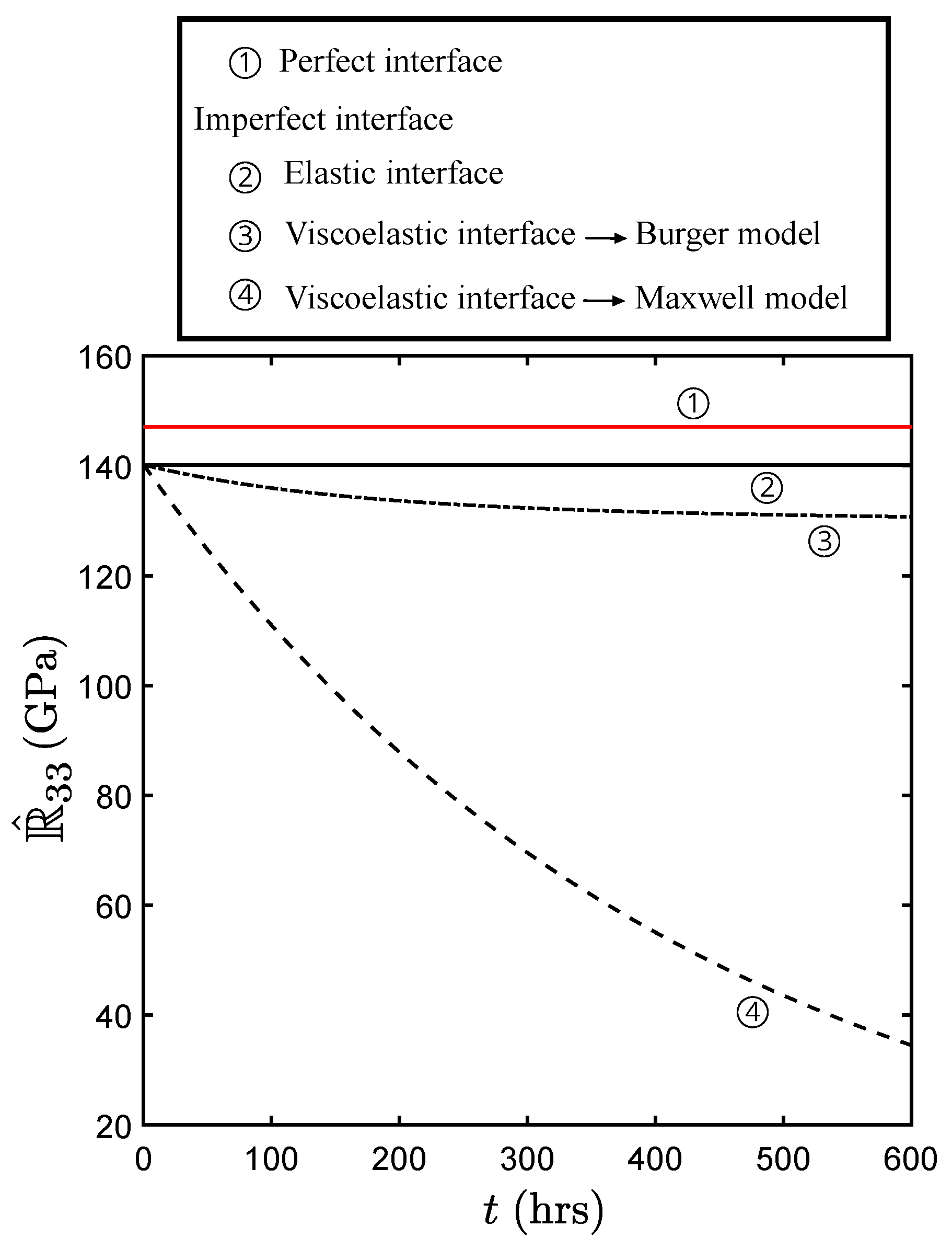
In this first example, the composite under study is assumed to have two elastic layers and we aim to variate the interfaces in order to study the influence of the viscoelastic effects. In the case of perfect contact conditions at the interfaces, we expect the occurrence of constant effective properties over the time. The same behavior must be observed in the case of elastic spring-type imperfect interfaces (see, e.g., [13,15]) in which no time is involved. The aforementioned cases are denoted by (1) and (2), respectively (see Figure 3). In addition, two further cases are analyzed, namely cases (3) and (4), corresponding to imperfect viscoelastic interfaces that consider a Burger’s model and a Maxwell’s model to respectively describe the viscoelastic behavior (see Figure 3).

The parameters for the two elastic layers (MAT 1 and MAT 2) and for the elastic interface (MAT 3) are given in

Table 1. Parameters for elastic materials.

	E (GPa)	$\mathit{\nu }$
MAT 1	150	0.3
MAT 2	72.04	0.35
MAT 3	2.5	0.25
MAT 4	34.8	0.443

, where E and $\nu$ stand for the Young’s modulus and Poisson’s ratio, respectively. In addition, the volumetric fraction of the layers is assumed to be 50%. Regarding the viscoelastic interfaces, the expressions for the creep compliance in Burger’s and Maxwell’s models are given respectively as follows (see [40,42]):

$$\begin{array}{c}\hfill S\left(t\right)=\frac{1}{E_0}+\frac{1}{E_1}\left(1-\exp \left(-\frac{E_1}{{\eta }_1}t\right)\right)+\frac{t}{{\eta }_2},\end{array}$$

(100)

and

$$\begin{array}{c}\hfill S\left(t\right)=\frac{1}{E_0}+\frac{t}{{\eta }_0}.\end{array}$$

(101)

The corresponding input parameters are displayed in

Table 2. Input data for the viscoelastic interfaces.

	${\mathit{E}}_0$ (GPa)	${\mathit{E}}_1$ (GPa)	${\mathit{\eta }}_0$ (GPa·h)	${\mathit{\eta }}_1$ (GPa·h)	${\mathit{\eta }}_2$ (GPa·h)	$\mathit{\nu }$
Maxwell’s model	2.5	-	50	-		0.25
Burger’s model	2.5	1.8	-	300	8000	0.25

.

Based on Equations (6a), (6b) and (10) of [10], we introduce the relaxation matrix ${\mathbb{K}}^{33}$, which contains the interface relaxation in normal and tangential directions to the interface, as follows:

$$\begin{array}{c}\hfill {\mathbb{K}}^{33}\left(t\right)=\frac{1}{r}\left[\begin{array}{ccc}\mu \left(t\right)& 0& 0\\ 0& \mu \left(t\right)& 0\\ 0& 0& \lambda \left(t\right)+2\mu \left(t\right)\end{array}\right]\end{array}$$

(102)

where $\mu \left(t\right)$ and $\lambda \left(t\right)$ are the time depended material properties of the linear viscoelastic isotropic interphase, and r is the interphase thickness herein given in meters.

Thus, Figure 3 shows the effective relaxation response of the composite material, given by the coefficient ${\widehat{\mathbb{R}}}_{33}$ for the four different cases outlined above. Here, we set the thickness value to $r={10}^{-3}$, and the variation of the effective properties is studied in the time interval $[0,600]$ (hrs).

It is worth mentioning that the data used in the calculation of cases (1) and (2) were deduced from [39], allowing us to compare the results with those presented in Table 1 of the same work. Figure 3 provides evidence of the good agreement between our findings. We point out that, in [39], the authors assume $\mu \left(t\right)+2\lambda \left(t\right)$ instead of $\lambda \left(t\right)+2\mu \left(t\right)$ (see Equation (55)); therefore, for the sake of comparison, we follow this scheme.

Additionally, we choose the parameters for cases (3) and (4) in order to obtain the same instant elastic response along the four studied cases. This means, graphically, having a common initial point for the graphs at $t=0$, which helps us to better visualize the influence of the imperfect viscoelastic interfaces compared to the elastic ones (see Figure 3).

As observed in Figure 3, regardless of the presence of elastic constituents, the effective properties show a time-dependent behavior when imperfect viscoelastic interfaces arise (see cases (3) and (4)). These results confirm that, within the present model, viscoelastic interfaces have a strong influence on the effective behavior of the composite materials. In addition, the differences observed depend on the viscoelastic model selected. For example, when the viscoelastic interface is modeled by the Burgers model, i.e., case (3), the relative variation of the effective relaxation modulus ${\widehat{\mathbb{R}}}_{33}$ at the fixed time $t=600$ hrs, in relation to the instant elastic response at $t=0$ hrs (see Figure 3) is $6.76$%, while, in the case of the Maxwell model, i.e., case (4), we have a variation that reaches $75.38$%. One justification for this behavior is provided by the relaxation representation of the two models, where the Maxwell model has a strong decrease with time.

5.2. Viscoelastic Composites with Viscoelastic Interfaces

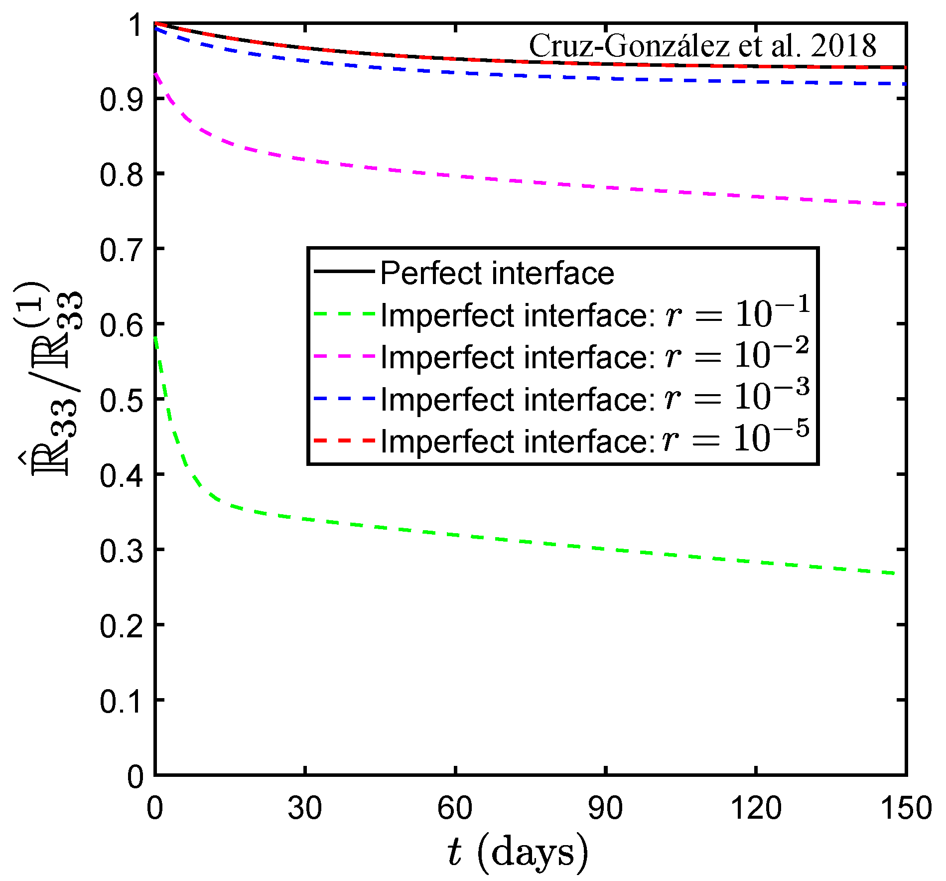
Now, in addition to have imperfect viscoelastic interfaces, some of the constituents are considered to behave as a viscoelastic material. In particular, we have a two-layered periodic medium (see Figure 2), where layer 1 presents a linear elastic behavior and layer 2, a linear viscoelastic one. The viscoelastic response of layer 2 is described by means of the Dischinger’s model (see [41,43]). This model assumes a time-dependent function, given by the form

$$\begin{array}{cc}\hfill & \phi (\tau ,t)=\exp (-\alpha t)-\exp (-\alpha \tau ),\hfill \end{array}$$

(103)

and thereby the relaxation functions for the viscoelastic constituent are defined for $\tau \le t$ as follows,

$$\begin{array}{cc}\hfill & {\mu }_2(\tau ,t)={\mu }_{20}\exp \left(\frac{{\mu }_{20}}{\alpha \beta }\phi (\tau ,t)\right),\hfill \end{array}$$

(104)

$$\begin{array}{c}\hfill {\lambda }_2(\tau ,t)=K-\frac{2}{3}{\mu }_2(\tau ,t),\end{array}$$

(105)

where K is the bulk elastic modulus and ${\mu }_{20}$ is a constant. Moreover, $\alpha$ and $\beta$ are parameters of the model.

Table 3. Parameters of Dischinger’s model.

K	${\mathit{\mu }}_{20}$	$\mathit{\alpha }·\mathit{\beta }$	$\mathit{\alpha }$	${\mathit{V}}_{\mathit{f}}^{\left({\mathcal{Y}}_1\right)}$
(MPa)	(MPa)	(MPa)	(day${}^{-1}$)	(Dimensionless)
10,000	8571	35,667	0.026	0.5

shows the input values for the Dischinger’s model. In addition, the correspondent Lame’s constants for the elastic layer 1 are taken by the relations

$$\begin{array}{cc}\hfill & {\mu }_1={\mu }_{20},{\lambda }_1=K-\frac{2}{3}{\mu }_{20},\hfill \end{array}$$

(106)

and we employ the Burger’s model used in Section 5.1 to describe the viscoelastic behavior of the interphase.

In Figure 4, the calculation of the normalized effective relaxation modulus ${\widehat{\mathbb{R}}}_{33}/{\mathbb{R}}_{33}^{\left(1\right)}$ is shown. The results are derived for different values of the interphase thickness r (see Equation (102)), and for the sake of comparison, we add the findings reported in [43], which refer to perfect interfaces. As observed, when the thickness approaches zero (see Equation (102)), the perfect interface condition is reached. This pattern is described in [9] as a consequence of the infinite values of the interface stiffness, which in our viscoelastic case corresponds to the interface relaxation given in Equation (102).

6. Numerical Results for Hierarchical Composites

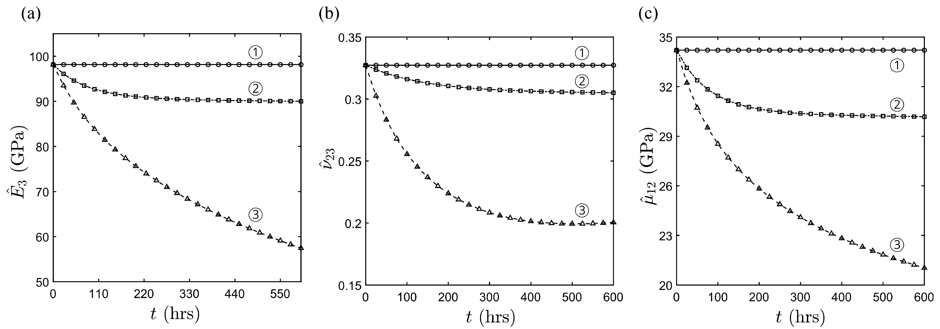
In this section, the influence that a hierarchical structure with viscoelastic constituents and imperfect interfaces has on the macroscopic response of a composite material is studied (see Figure 5). At the ${\epsilon }_1$-structural level, we have a wavy laminated composite involving imperfect viscoelastic interfaces (see Figure 5b). In addition, one of these constituents is at the same time a spherical reinforced composite material, where perfect contact conditions are considered between the matrix and the inclusion (see Figure 5c).

For this purpose, we compute the effective coefficients at the smallest scale (${\epsilon }_2$-structural level) by means of the numerical approach developed in [44,45]. Then, the theoretical results presented in Section 4.2 are considered to solve analytically the local problems at the ${\epsilon }_1$-structural level for a wavy laminate composite with imperfect interfaces and anisotropic components.

It is worth mentioning that four different constituents are involved in the calculation, i.e., the spherical inclusions and the matrix which together made up layer 1; in addition, we have layer 2 and the interphase. Taking this into consideration, we study three different combinations of the parameters (see case (1), (2) and (3) in

Table 4. Cases studied in this section.

	MAT 1	MAT 2	MAT 3	MAT 4	Maxwell’s Model	Burger’s Model (a)
Case (1)	Matrix	Layer 2	Interface	Inclusion	-	-
Case (2)	Matrix	Layer 2	Interface	-	-	Inclusion
Case (3)	Matrix	Layer 2	-	-	Interface	Inclusion

). Most of the material input data are taken from Section 5.1. In contrast, we now consider the relaxation representation of Burger’s model (a)

$$\begin{array}{c}\hfill E_m\left(t\right)=G_1\exp \left(-\frac{t}{{\eta }_{\sigma ,1}}\right)+G_2\exp \left(-\frac{t}{{\eta }_{\sigma ,2}}\right),\end{array}$$

(107)

whose parameters are given in

Table 5. Parameters for the relaxation representation of the Burger’s model.

	${\mathit{G}}_1$ (GPa)	${\mathit{G}}_2$ (GPa)	${\mathit{\eta }}_{\mathit{\sigma },1}$ (h)	${\mathit{\eta }}_{\mathit{\sigma },2}$ (h)	$\mathit{\nu }$
Burger’s model (a)	13.4	21.4	7742.22	68.8863	0.443

.

The volume fractions at the different levels of organization are assumed to be $V_f^{\left(\mathrm{inclusion}\right)}=0.3$, $V_f^{\left(\mathrm{matrix}\right)}=0.7$ and $V_f^{\left(\mathrm{layer}2\right)}=0.2$. In addition, the stratified function, ${\rho }^{\left(y\right)}:{\mathbb{R}}^3\to \mathbb{R}$, defined as follows:

$$\begin{array}{cc}\hfill & {\rho }^{\left(y\right)}(x_1,x_2,x_3)=x_3-H\sin \left(\frac{2\pi x_2}{L}\right),\hfill \end{array}$$

(108)

is employed to describe the wavy effect at the ${\epsilon }_1$-structural level (see Figure 5b). In particular, we consider the ratio $H/L=0.25$.

In Figure 6, we display the results in the calculation of the effective viscoelastic properties, ${\widehat{E}}_3$, ${\widehat{\nu }}_{23}$, and ${\widehat{\mu }}_{12}$, which represent the Young modulus, Poisson ratio, and shears modulus, respectively. The findings are derived for the three different combinations of the parameters given in Table 4. In this regard, case (1) stands for a hierarchical composite in which all the constituents, as well as the imperfect interface at the ${\epsilon }_1$-structural level, behave as elastic materials. Then, as observed in Figure 6, constant graphs are obtained in this situation. In relation to the remaining cases, Figure 6 shows how the viscoelastic behavior of the spherical inclusions (case (2)) and spherical inclusions–interface (case (3)) have an influence on the macroscopic effective response of the hierarchical composite, generating time-dependent graphs. For instance, in case (2), the relative variation of the effective Young modulus ${\widehat{E}}_3$ at $t=300$ hrs in relation to the instant elastic response at $t=0$ hrs (see Figure 6a) is given by $7.81$%, while, in case (3), we have a variation that reaches $29.04$%, providing quantitative evidence of the differences reported in the calculations.

7. Conclusions

In this work, the first attempt to integrate, on the one hand, the imperfect interface approach developed in [17] for soft and hard materials, and on the other hand a methodology for addressing the problem in the case of hierarchical viscoelastic materials with periodic heterogeneous structures and imperfect interfaces was proposed. In the first part of the manuscript we generalized some of the results of the problem of two bodies in adhesion in which the adhesive and some of the adherents exhibit a viscoelastic effect, and soft viscoelastic interface law are deduced at zero-order in the time domain, corresponding with the viscoelastic counterpart of the classical spring-type imperfect elastic interface. So then, the problem for non-aging linear viscoelastic composite material with hierarchical structure and imperfect viscoelastic interfaces was addressed via a three-scale Asymptotic Homogenization Method (AHM) accounting for the procedure developed in [27]. Some of the existing results in the elastic composite with imperfect interfaces are used to solve the local problems and calculate the effective properties in a two-dimensional framework. Finally, we showed the potential of the proposed asymptotic homogenization procedure by modeling the effective properties of laminate structures with rectangular and wavy layers. In the former, the influence of imperfect interfaces on the effective behavior of the composite was studied, whereas in the later, we considered a hierarchical structure with spherical inclusions and calculate the effective properties accounting for the stratified functions.

It should be added as a drawback of the approach taken in Section 6 that the model does not take into account the hierarchy order between the imperfect interface at the ${\epsilon }_1$-structural level and the smallest scale (${\epsilon }_2$-structural level), which deserves to be analyzed in a future work.

In addition, several potential extensions can be done. For instance, we may consider imperfect viscoelastic interfaces in more general structures than laminated ones and include the interfaces at both structural levels to study the damage propagation in materials with periodic microstructure and viscoelastic interphases (see, e.g., [29,46,47,48,49]).

References

- Ouaer, H.; Gareche, M. The rheological behaviour of a water-soluble polymer (HEC) used in drilling fluids. J. Braz. Soc. Mech. Sci. Eng. 2018, 40, 380. [Google Scholar] [CrossRef]
- Rivas, B.L.; Urbano, B.F.; Sánchez, J. Water-Soluble and Insoluble Polymers, Nanoparticles, Nanocomposites and Hybrids With Ability to Remove Hazardous Inorganic Pollutants in Water. Front. Chem. 2018, 6, 320. [Google Scholar] [CrossRef] [PubMed] [Green Version]
- Zhu, X.y.; Wang, X.; Yu, Y. Micromechanical creep models for asphalt-based multi-phase particle-reinforced composites with viscoelastic imperfect interface. Int. J. Eng. Sci. 2014, 76, 34–46. [Google Scholar] [CrossRef]
- Escarpini Filho, R.S.; Marques, S.P.C.; Federal University of Alagoas, Brazil. A Model for Homogenization of Linear Viscoelastic Periodic Composite Materials with Imperfect Interface. Lat. Am. J. Solids Struct. 2016, 13, 2706–2735. [Google Scholar] [CrossRef] [Green Version]
- Hashemi, R. On the overall viscoelastic behavior of graphene/polymer nanocomposites with imperfect interface. Int. J. Eng. Sci. 2016, 105, 38–55. [Google Scholar] [CrossRef]
- Daridon, L.; Licht, C.; Orankitjaroen, S.; Pagano, S. Periodic homogenization for Kelvin-Voigt viscoelastic media with a Kelvin-Voigt viscoelastic interphase. Eur. J. Mech.-A/Solids 2016, 58, 163–171. [Google Scholar] [CrossRef] [Green Version]
- Schöneich, M.; Dinzart, F.; Sabar, H.; Berbenni, S.; Stommel, M. A coated inclusion-based homogenization scheme for viscoelastic composites with interphases. Mech. Mater. 2017, 105, 89–98. [Google Scholar] [CrossRef]
- Benveniste, Y. The effective mechanical behaviour of composite materials with imperfect contact between the constituents. Mech. Mater. 1985, 4, 197–208. [Google Scholar] [CrossRef]
- Hashin, Z. Thermoelastic properties of fiber composites with imperfect interface. Mech. Mater. 1990, 8, 333–348. [Google Scholar] [CrossRef]
- Hashin, Z. Composite materials with viscoelastic interphase: Creep and relaxation. Mech. Mater. 1991, 11, 135–148. [Google Scholar] [CrossRef]
- Hashin, Z. Thin interphase/imperfect interface in elasticity with application to coated fiber composites. J. Mech. Phys. Solids 2002, 50, 2509–2537. [Google Scholar] [CrossRef]
- Raffa, M.L. Micromechanical Modeling of Imperfect Interfaces and Applications. Ph.D. Thesis, University of Rome “Tor Vergata” in Joint Supervision with Aix-Marseille University, Rome, Italy, 2015. [Google Scholar]
- Otero, J.A.; Rodríguez-Ramos, R.; Monsivais, G. Computation of effective properties in elastic composites under imperfect contact with different inclusion shapes. Math. Methods Appl. Sci. 2017, 40, 3290–3310. [Google Scholar] [CrossRef]
- Guinovart-Sanjuán, D.; Vajravelu, K.; Rodríguez-Ramos, R.; Guinovart-Díaz, R.; Bravo-Castillero, J.; Lebon, F.; Sabina, F.J. Analysis of effective elastic properties for shell with complex geometrical shapes. Compos. Struct. 2018, 203, 278–285. [Google Scholar] [CrossRef] [Green Version]
- Brito-Santana, H.; Medeiros-Thiesen, J.L.; de Medeiros, R.; Mendes-Ferreira, A.; Rodríguez-Ramos, R.; Tita, V. Multiscale analysis for predicting the constitutive tensor effective coefficients of layered composites with micro and macro failures. Appl. Math. Model. 2019, 75, 250–266. [Google Scholar] [CrossRef]
- Wang, G.; Tu, W.; Chen, Q. Homogenization and localization of imperfectly bonded periodic fiber-reinforced composites. Mech. Mater. 2019, 139, 103178. [Google Scholar] [CrossRef]
- Rizzoni, R.; Dumont, S.; Lebon, F.; Sacco, E. Higher order model for soft and hard elastic interfaces. Int. J. Solids Struct. 2014, 51, 4137–4148. [Google Scholar] [CrossRef]
- Rizzoni, R.; Dumont, S.; Lebon, F.; Sacco, E. Higher order adhesive effects in composite beams. Eur. J. Mech.-A/Solids 2021, 85, 104108. [Google Scholar] [CrossRef]
- Sanchez-Palencia, E.; Sanchez-Hubert, J. Introduction aux Méthodes Aymptotiques et á l’homogénéisation; Elsevier Masson: Paris, France, 1992. [Google Scholar]
- Geymonat, G.; Hendili, S.; Krasucki, F.; Vidrascu, M. Numerical validation of an homogenized interface model. Comput. Methods Appl. Mech. Eng. 2014, 269, 356–380. [Google Scholar] [CrossRef] [Green Version]
- Lebon, F.; Dumont, S.; Rizzoni, R.; López-Realpozo, J.C.; Guinovart-Díaz, R.; Rodríguez-Ramos, R.; Bravo-Castillero, J.; Sabina, F.J. Soft and hard anisotropic interface in composite materials. Compos. Part B Eng. 2016, 90, 58–68. [Google Scholar] [CrossRef] [Green Version]
- Raffa, M.L.; Lebon, F.; Vairo, G. Normal and tangential stiffnesses of rough surfaces in contact via an imperfect interface model. Int. J. Solids Struct. 2016, 87, 245–253. [Google Scholar] [CrossRef]
- Dumont, S.; Rizzoni, R.; Lebon, F.; Sacco, E. Soft and hard interface models for bonded elements. Compos. Part B Eng. 2018, 153, 480–490. [Google Scholar] [CrossRef] [Green Version]
- Serpilli, M.; Rizzoni, R.; Lebon, F.; Dumont, S. An asymptotic derivation of a general imperfect interface law for linear multiphysics composites. Int. J. Solids Struct. 2019, 180–181, 97–107. [Google Scholar] [CrossRef] [Green Version]
- Dumont, S.; Serpilli, M.; Rizzoni, R.; Lebon, F. Numerical Validation of Multiphysic Imperfect Interfaces Models. Front. Mater. 2020, 7, 158. [Google Scholar] [CrossRef]
- Lebon, F.; Rizzoni, R.; Ronel-Idrissi, S. Asymptotic analysis of some nonlinear soft thin layers. Comput. Struct. 2004, 82, 1929–1938. [Google Scholar] [CrossRef] [Green Version]
- Cruz-González, O.L.; Ramírez-Torres, A.; Rodríguez-Ramos, R.; Penta, R.; Bravo-Castillero, J.; Guinovart-Díaz, R.; Merodio, J.; Sabina, F.J.; Lebon, F. A hierarchical asymptotic homogenization approach for viscoelastic composites. Mech. Adv. Mater. Struct. 2020, 28, 2190–2201. [Google Scholar] [CrossRef]
- Dumont, S.; Lebon, F.; Rizzoni, R. An asymptotic approach to the adhesion of thin stiff films. Mech. Res. Commun. 2014, 58, 24–35. [Google Scholar] [CrossRef] [Green Version]
- Bonetti, E.; Bonfanti, G.; Lebon, F.; Rizzoni, R. A model of imperfect interface with damage. Meccanica 2017, 52, 1911–1922. [Google Scholar] [CrossRef]
- Nguetseng, N.; Sánchez-Palencia, E. Stress concentration for defects distributed near a surface. Stud. Appl. Mech. 1985, 12, 55–74. [Google Scholar]
- Geymonat, G.; Krasucki, F.; Hendili, S.; Vidrascu, M. The matched asymptotic expansion for the computation of the effective behavior of an elastic structure with a thin layer of holes. Int. J. Multiscale Comput. Eng. 2011, 9, 529–542. [Google Scholar] [CrossRef]
- Lebon, F.; Rizzoni, R. Asymptotic analysis of a thin interface: The case involving similar rigidity. Int. J. Eng. Sci. 2010, 48, 473–486. [Google Scholar] [CrossRef] [Green Version]
- Geymonat, G.; Hendili, S.; Krasucki, F.; Vidrascu, M. Matched asymptotic expansion method for a homogenized interface model. Math. Model. Methods Appl. Sci. 2014, 24, 573–597. [Google Scholar] [CrossRef] [Green Version]
- Ciarlet, P.G. Mathematical elasticity, volume I: Three-dimensional elasticity. Acta Appl. Math. 1990, 18, 190–195. [Google Scholar] [CrossRef]
- Dumont, S.; Lebon, F.; Raffa, M.L.; Rizzoni, R. Towards nonlinear imperfect interface models including micro-cracks and smooth roughness. Ann. Solid Struct. Mech. 2017, 9, 13–27. [Google Scholar] [CrossRef] [Green Version]
- Christensen, R.M. Theory of Viscoelasticity—An Introduction, 2nd ed.; Academic Press: Cambridge, MA, USA; New York, NY, USA, 1982. [Google Scholar]
- Penta, R.; Gerisch, A. Investigation of the potential of asymptotic homogenization for elastic composites via a three-dimensional computational study. Comput. Vis. Sci. 2015, 17, 185–201. [Google Scholar] [CrossRef]
- Penta, R.; Gerisch, A. The asymptotic homogenization elasticity tensor properties for composites with material discontinuities. Contin. Mech. Thermodyn. 2017, 29, 187–206. [Google Scholar] [CrossRef] [Green Version]
- Guinovart-Sanjuán, D.; Rizzoni, R.; Rodríguez-Ramos, R.; Guinovart-Díaz, R.; Bravo-Castillero, J.; Alfonso-Rodríguez, R.; Lebon, F.; Dumont, S.; Sevostianov, I.; Sabina, F.J. Behavior of laminated shell composite with imperfect contact between the layers. Compos. Struct. 2017, 176, 539–546. [Google Scholar] [CrossRef] [Green Version]
- Mainardi, F.; Spada, G. Creep, relaxation and viscosity properties for basic fractional models in rheology. Eur. Phys. J. Spec. Top. 2011, 193, 133–160. [Google Scholar] [CrossRef] [Green Version]
- Maghous, S.; Creus, G.J. Periodic homogenization in thermoviscoelasticity: Case of multilayered media with ageing. Int. J. Solids Struct. 2003, 40, 851–870. [Google Scholar] [CrossRef]
- Lakes, R.S. Viscoelastic Materials; Cambridge University Press: Cambridge, UK, 2009. [Google Scholar]
- Cruz-González, O.L.; Rodríguez-Ramos, R.; Otero, J.A.; Bravo-Castillero, J.; Guinovart-Díaz, R.; Martínez-Rosado, R.; Sabina, F.J.; Dumont, S.; Lebon, F.; Sevostianov, I. Viscoelastic effective properties for composites with rectangular cross-section fibers using the asymptotic homogenization method. In Generalized Models and Non-Classical Approaches in Complex Materials 1; Altenbach, H., Pouget, J., Rousseau, M., Collet, B., Michelitsch, T., Eds.; Advanced Structured Materials; Springer International Publishing: Cham, Switzerland, 2018; Volume 89, pp. 203–222. [Google Scholar] [CrossRef] [Green Version]
- Cruz-González, O.L.; Rodríguez-Ramos, R.; Otero, J.A.; Ramírez-Torres, A.; Penta, R.; Lebon, F. On the effective behavior of viscoelastic composites in three dimensions. Int. J. Eng. Sci. 2020, 157, 103377. [Google Scholar] [CrossRef]
- Cruz-González, O.L.; Ramírez-Torres, A.; Rodríguez-Ramos, R.; Otero, J.A.; Penta, R.; Lebon, F. Effective behavior of long and short fiber-reinforced viscoelastic composites. Appl. Eng. Sci. 2021, 6, 100037. [Google Scholar] [CrossRef]
- Rekik, A.; Nguyen, T.T.N.; Gasser, A. Multi-level modeling of viscoelastic microcracked masonry. Int. J. Solids Struct. 2016, 81, 63–83. [Google Scholar] [CrossRef]
- Fantoni, F.; Bacigalupo, A.; Paggi, M.; Reinoso, J. A phase field approach for damage propagation in periodic microstructured materials. Int. J. Fract. 2020, 223, 53–76. [Google Scholar] [CrossRef] [Green Version]
- Shen, N.; Peng, M.Y.; Gu, S.T.; Hu, Y.G. Effects of the progressive damage interphase on the effective bulk behavior of spherical particulate composites. Acta Mech. 2021, 232, 423–437. [Google Scholar] [CrossRef]
- Raffa, M.L.; Rizzoni, R.; Lebon, F. A Model of Damage for Brittle and Ductile Adhesives in Glued Butt Joints. Technologies 2021, 9, 19. [Google Scholar] [CrossRef]
Figure 1.
(a) Reference configuration for the viscoelastic composite material with the h-thick interphase; (b) rescaled configuration; and (c) final configuration or limit interface problem (zero-thick interphase).
Figure 2.
(a) Macroscale, (b) -structural level, (c) Microscale. Viscoelastic composite material with a rectangular geometrical configuration and imperfect interfaces.
Figure 3.
Calculation of the effective relaxation modulus by means of Equation (93). We set the interphase thickness . Note that cases 2, 3, and 4 refer to imperfect interfaces.
Figure 4.
Computations of the normalized effective relaxation modulus by means of Equation (93) for different interphase thickness. The results given in [43] for perfect interfaces are shown as reference. In the computations, we consider , which represents a medium with non-aging.
Figure 5.
(a) Macroscale, (b) -structural level/Mesoscale, (c) -structural level/Microscale. Hierarchical composite material with imperfect viscoelastic interfaces at the -structural level.
Figure 6.
Computations of the effective (a) Young modulus; (b) Poisson ratio; and (c) shear modulus for the hierarchical structure shown in Figure 5. The numbers (1–3) in the figure correspond to the studied cases given in Table 4. We have averaged the results over in , and we set the interphase thickness to .