Novel Model for the Angle and Skewness Dependent Transmission Behavior of Step-Index Polymer Optical Fiber


1
Polymer Optical Fiber Application Center, Technische Hochschule Nürnberg Georg Simon Ohm, Wassertorstraße 10, 90489 Nürnberg, Germany
2
Institute of Microwaves and Photonics (LHFT), Friedrich-Alexander-Universität Erlangen-Nürnberg, Wetterkreuz 15, 91058 Erlangen, Germany
*
Author to whom correspondence should be addressed.
Fibers 2018, 6(3), 65; https://0-doi-org.brum.beds.ac.uk/10.3390/fib6030065
Submission received: 10 August 2018
/
Revised: 3 September 2018
/
Accepted: 4 September 2018
/
Published: 5 September 2018
(This article belongs to the Special Issue Plastic Optical Fibers)
Abstract
:Step-index polymer optical fibers (SI-POFs) are deployed in both sensing and data transmission systems. The optical transmission behavior of these fibers is complex and affected by intrinsic influences like modal dispersion, scattering and attenuation as well as extrinsic influences like the launching condition and the angular sensitivity of the receiver. Since a proper modeling of the transmission behavior is important in order to evaluate the suitability of the fiber for a specific application, we present a novel model for step-index multi-mode fibers (SI-MMFs) which considers all the previously mentioned impacts. Furthermore, the model differentiates scattering and attenuation for propagating rays not only by their propagating angle but also by the skewness . It is therefore possible to distinguish between guided, tunneling and refracted modes. The model uses scatter and attenuation data from previously published measurements of an SI-POF and computes the impulse response of the transmission system which is transferred to the frequency domain to derive the amplitude and phase response. A possible application for SI-POF is the length or strain measurement of the fiber by measuring the phase of a harmonically modulated signal. These sensors rely on a linear relation between the length of the fiber and the phase of the modulated signal. We demonstrate the application of the model by simulating the length measurement error that occurs for these sensors by obtaining the phase response for the corresponding optical transmission system. Furthermore, we will demonstrate the flexibility of the model by varying several influences including the excitation of different mode categories and evaluate the impact on the measurement error. Finally, we compare the simulated length error derived from the model to real data obtained from a cutback measurement. An implementation of the model, which was used for all simulations in this paper, is publicly available.
1. Introduction
Multi-mode fibers (MMFs) like polymer optical fibers (POFs) differ from single-mode fibers (SMFs) and few-mode fibers by their potential modeling approaches. Due to the limited number of modes, the latter ones can be modeled by solving the wave equation for each possible mode individually. However, this approach is unfeasible for MMFs because of their large number of modes. For example, the typical step-index polymer optical fiber (SI-POF) can guide several million modes. Common modeling approaches for MMFs include ray tracing simulations and the power flow equation (PFE) [1,2,3]. Both approaches are based on optical powers, which makes it impossible to consider interference between different modes, which occurs due to the periodicity of the electro-magnetic field. While there are approaches based on the propagation of the elctro-magnetic field in MMFs [4,5], working with optical powers is sufficient for POF since it is known not to maintain the polarization for fibers longer than ≈50 cm [6]. The PFE has been used to derive the transfer function of MMFs depending on several parameters [7]. Furthermore, the necessary coefficients describing the mode conversion and attenuation have been measured for SI-POF as well [8]. However, the separate measurement of attenuation and mode conversion caused by scattering is not without problems. The measurement of one effect is always influenced by the other since none of them can be avoided completely. This is especially true for POF since it faces significantly more scattering than a glass optical fiber (GOF).
An additional drawback of both ray tracing and the PFE is the neglect of a ray’s skewness, which makes it impossible to distinguish between tunneling and refracted modes as proposed by Snyder and Love [9]. Figure 1a shows two rays with the same propagation angle . The red ray is a meridional ray since it crosses the optical axis. It can be seen that the trajectory of the ray changes significantly when its origin is shifted towards the edge of the fiber (black ray), even though remains constant. The resulting ray is called a skew ray. The difference between both rays can be described by the skewness , which is the angle between the projection of a ray’s trajectory on the fiber’s front surface and the tangent at the point of reflection and is depicted in Figure 1b. Closely related to and is a third angle (Figure 1a), which is the angle between the ray and the normal to the surface at the point of reflection. can be expressed depending on and :
Due to the relation between the three angles, it is sufficient to consider only two of them to distinguish the different mode categories. For the further discussion, we choose and . Figure 2 shows the possible mode categories with respect to the chosen angles. It is well known that a mode can only be guided if is smaller than the maximum angle , for which total internal reflection occurs:
is the refractive index of the core of the fiber and is the refractive index of the cladding. If exceeds , the mode category depends on . Similar to , a minimum angle is defined:
If exceeds , the mode is a tunneling mode and suffers therefore from a higher attenuation than a guided mode. If is smaller than , the mode is a refracted mode. The attenuation of refracted modes is even higher than for tunneling modes, which is why they only contribute to the transmission behavior of very short fibers.
The number of reflections at the core-cladding interface, which a ray faces while propagating along the fiber, depends on the skewness as can be seen from Figure 1a. As a consequence, the scattering experienced by a mode depends on the skewness as well. The transmission behavior of a step-index multi-mode fiber (SI-MMF) therefore does not only depend on the angular power distribution of the light source over , but also on the power distribution over . We propose a new fiber model for SI-MMF that is capable of considering the dependency of both attenuation and scattering on both angles. This allows us to investigate the influence of the angular power distribution and the different mode categories on specific applications by evaluating the phase and amplitude response obtained from the impulse response of the simulated optical transmission system.
We have previously proposed an optical strain sensor based on an SI-POF [10,11]. An intensity-modulated LED is used to excite the fiber with a fixed modulation frequency and the strain of the fiber can be monitored by measuring the modulation phase at the end of the fiber as shown in Figure 3.
When the length of the fiber is changed by , the modulation phase experiences a phase shift . In an ideal fiber, which is free from dispersion, scattering and other parasitic influences, the modulation phase at a specific position has a linear dependency on the position z. As a result, the shift of the modulation phase caused by the elongation of an ideal fiber is proportional to the length change:
However, in a real fiber, the development of the modulation phase along the fiber is not linear to the position z and therefore not linear to the length change as well. A measured phase change can correspond to a different length change at a specific position z than it does at another. The modulation phase at the end of the fiber is exposed to additional influences when the fiber is actually strained as we have recently investigated [12]. However, in order to avoid a measurement error, it is crucial to know how the real development of the modulation phase along the fiber differs from the ideal modulation phase.
We will demonstrate the application of the model by simulating the nonlinear development of the modulation phase along the fiber. For this purpose, we simulate the impulse responses at discrete positions along the sensing fiber. The impulse responses are then transferred to the frequency domain via a Fourier transform. The argument of the obtained frequency responses are the phase responses, which allows us to predict the development of the modulation phase along the sensing fiber at arbitrary modulation frequencies. Since the sensor is based on an SI-POF, the model employs scatter data we have obtained from a previously performed scatter and attenuation measurement of an SI-POF described in [13]. The model itself is independent from the actual fiber type and can model any kind of SI-MMF as long as the required scatter and attenuation data for the specific fiber type are available.
In order to study the the impact on the development of the modulation phase, we will vary the following simulation parameters:
- Launching condition,
- Mode categories,
- Angular sensitiviy of the receiver,
- Modulation frequency.
Finally, we will compare the simulated development of the modulation phase along the fiber to real values obtained from a cutback measurement.
2. Materials and Methods
2.1. Fiber Model
The model computes the impulse response of an optical transmission system including the light source, the fiber and the optical receiver. For the evaluation of the suitability of the transmission system for a specific application, the impulse response has to be transferred to the frequency domain by a Fourier transform. A brief introduction to the required system theoretical principles can be found in Appendix A, which also includes the definition of an optical impulse response in order to consider the dimensions of the involved physical quantities properly.
2.1.1. General Description of the Model
The proposed fiber model is based on a description of the power distribution at discrete, equidistant positions z along the fiber depending on , and the time t. Each position is represented by a matrix M, with n being the position index. A matrix consists of a two-dimensional array with matrix cells MC with each cell being responsible for a specific combination of a range (index ) and a range (index ). As indicated in Figure 4, each matrix cell contains two elements:
- Cell power (CP),
- Cell scatter matrix (CSM).
The cell power (CP) describes the power over time with which a cell is being excited and can occur in two different shapes. The first one is an Dirac-shaped power pulse as described by Equation (A3) and is used to excite the cells of the first matrix (). The second one is called cell impulse response (CIR) and describes a discrete power over time with the time index k. It is used for the excitation of all subsequent matrices (). The cell scatter matrix describes how much of the power of the current cell is transferred into each cell of the next matrix M. The model does not distinguish between attenuation and scattering, since both are included jointly in the scatter matrices. While the cell scatter matrices are unique to each cell of a matrix, the total set of CSMs are identical for each matrix and therefore independent from n. As a result, there is only one set of cell scatter matrices that is referenced by each matrix.
The model requires two different types of data as input:
- Distribution of the initial excitation,
- Cell scatter matrices.
The initial power distribution describes the power distribution over and at and and depends on the angular and positional power distribution of the light source. We have derived the mathematical equations to describe the power distribution of a light source over and previously [14]. Furthermore, the angular conversion and Fresnel losses, which occur when the light enters the fiber, have to be considered. Both were covered in [14] as well. The discrete power , exciting each cell, can be derived from the continuous power distribution of the total excitation :
with , , and being the angular boundaries of the excited matrix cell. As discussed in Appendix A, the transmission system has to be excited with a Dirac-shaped light pulse of a certain energy . As a consequence, each matrix cell has to be excited with a Dirac-impulse containing an energy which is proportional to :
is the total power exciting the system:
with , , and being the boundaries of the total angular range considered by the model. As indicated by Equation (5), the model works with powers and not power densities. For reasons discussed in Section 2.1.3, the angular step widths of the cells are not equidistant. Working with absolute powers makes the model therefore more transparent and the power exchange between the cells during each matrix transition easier to model. The dimensions of the matrix represent the number of discrete angular steps over and and can freely be chosen. The same holds for the angular boundaries of each cell and the total angular ranges that are considered by the model. The only requirement is a valid set of scatter matrices for the chosen parameters. The cell scatter matrices are obtained from measurements of a fiber of a certain length L as described in [13]. Hence, the length between two matrices M and M is also defined by the cell scatter matrices.
2.1.2. Propagation Algorithm
The propagation algorithm that describes the evolution of the power distribution along the fiber is depicted in Algorithm 1. The first step is the initial excitation of the cell powers of the first matrix . Each cell is excited with a Dirac-impulse (Equation A3) containing the energy :
Once this is accomplished, the main loop, which cycles through the matrices until the desired fiber length has been reached, starts. Whenever a subsequent matrix is initialized, the cell impulse response of each cell is initialized with a given number of steps K and a minimum and maximum time that can occur at the position in the fiber that is related to the current matrix. The power of each interval of is set to 0. The task of the next loop is to iterate all matrix cells of the current matrix M. In case of the first matrix (), the excitation power of the considered cell is transferred to the next matrix according to the scatter matrix of the cell. In all other cases (), the power of each of the K time intervals of the cell impulse response has to be transferred to the next matrix according to the scatter matrix of the current cell. A detailed description of the scattering process is given in Section 2.1.3. When all required matrix transitions are completed, Fresnel losses occurring at the end of the fiber are applied to the cell impulse responses. By applying angular filters, specific receiver characteristics can be considered. The next step is to sum up the cell impulse responses of all matrix cells of the final matrix to obtain the total impulse response that describes the whole transmission system. Finally, the obtained impulse response is normalized with respect to the exciting energy to obtain the normalized impulse response as described in Appendix A.
| Algorithm 1 Simulation of the power propagation in the fiber. |
|
2.1.3. Details of the Available Implementation
An implementation of the proposed model is available on GitHub [15] along with the required scatter matrices of a standard SI-POF with a diameter of 1 . Instructions on how to build and use the model are provided in the file README.md. The model applies scattering and attenuation to a propagating light wave depending on the used cell scatter matrices. As a result, some properties of the model like the angular boundaries of the matrix cells (, , and ) and the distance between two matrices are defined by the CSMs. The properties of the CSMs in turn depend on the measurement setup, with which the scatter data were obtained. In this section, we will give a brief overview of the measurement setup, which was used to obtain the CSMs used in this paper and the subsequent adjustments of the model.
The scatter data we use for the model were obtained from a standard SI-POF with a diameter of 1 and a length of cm. As a result, the distance between two discrete propagation lengths represented by and is cm as well. A detailed description of the measurement setup can be found in [13].
Angular Bounds of the Cells
During the measurements, the fiber was excited with a collimated laser beam under different angles between the optical axis and the collimated beam outside the fiber. Since the measurements were carried out for equidistant steps for the angle , the steps for inside the fiber were not equidistant. The central angle of a matrix cell with the index is therefore
with . The measurement was performed with steps and a maximum angle of 85°, resulting in a step size of 1°. However, in order to increase the resolution of the scatter matrices, the data were interpolated for a step size of 0.1°, resulting in a scatter matrix with rows. The cell bounds for can be expressed as
and
There are two exceptions at the boundaries with
and
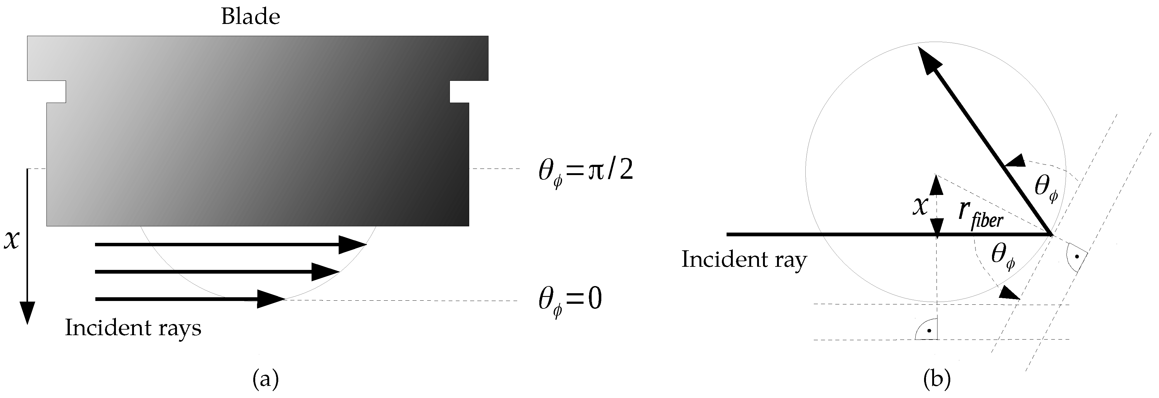
During the measurements, the skewness of the excited modes was varied by partly covering the fiber’s front surface with a movable blade as shown in Figure 5a. The skewness of a ray can be influenced by a lateral shift x, which is the distance between the incident ray and center of the fiber as indicated in Figure 5b. The blade covered at least the upper half of the front surface () and was moved downwards in 5 steps until the full front surface was covered (), with being the radius of the core of the fiber. For follows measurements, since the measurement of the completely covered front surface was unnecessary for obvious reasons. As a result, the obtained cell scatter matrices have columns with . As mentioned before, is the number of discrete angular steps of the model for and is given by the provided cell scatter matrices. During the measurements, the lower limit of the excited range was independent from the position of the blade and was always . The upper limit can be expressed depending on x or respectively:
The scatter data for the range of a specific cell was derived from the difference of two measurements with neighboring blade positions. The maximum value of the range of a cell can be obtained from Equation (14) as well. The minimum value can be expressed as:
Cell Impulse Response
The model uses cell impulse responses (), representing a power over K time intervals, to excite all matrices but the first. The minimum and maximum time covered by a particular depends on the position index n of the matrix but is independent of the particular cell of the matrix or and , respectively:
is the speed of light in vacuum. The influence of chromatic dispersion on the pulse broadening in SI-POF is negligible in comparison to the influence of modal dispersion. However, chromatic dispersion does affect the group velocity of modulated signals. Therefore, we consider the refractive group index . The temporal boundaries of () are set to the extremal values that can occur in the current matrix. As a result, a power of any ray which is scattered into a specific cell of a matrix can be recognized by (), independent of its previous path.
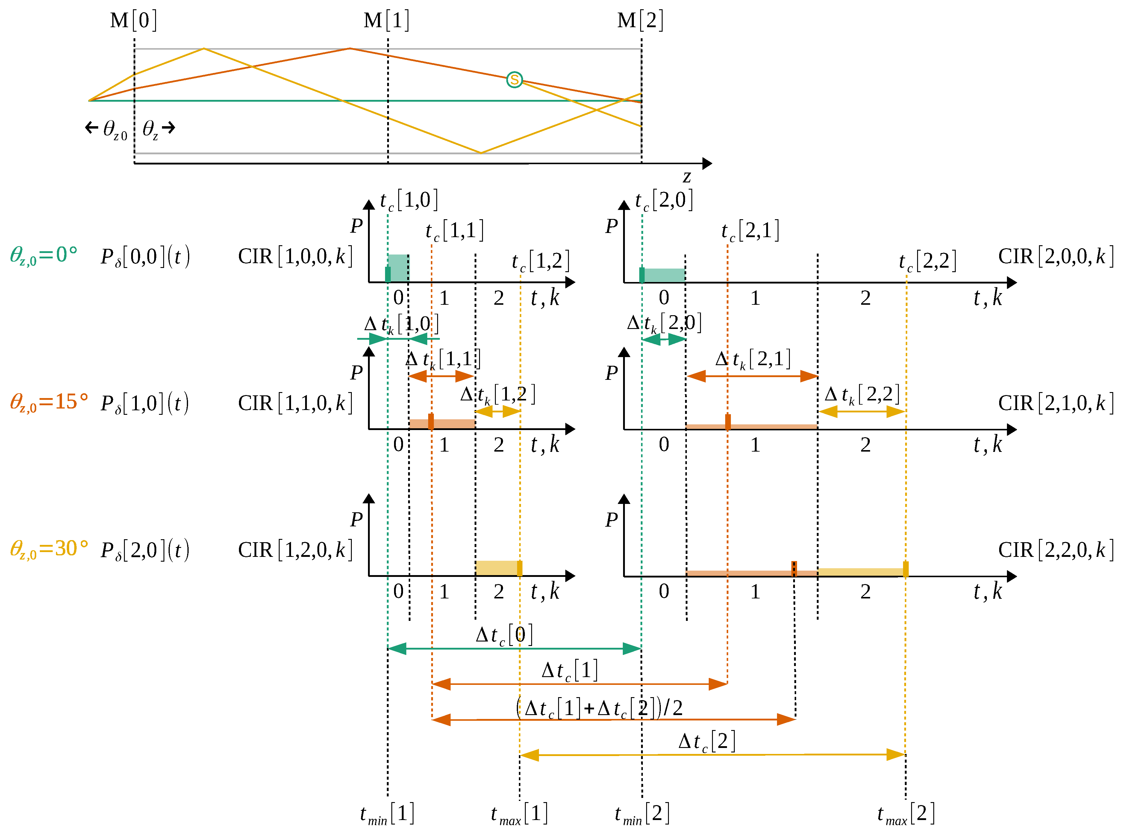
A simplified example with three matrices is shown in Figure 6 to illustrate the application of the CIRs in the model. Since this example involves CIRs of different matrix cells and of different matrices, we need to expand the corresponding notation to (. The example uses only three rays with the angles (green) , 15 (red) and 30 (yellow). Therefore, the number of discrete steps over is and . We choose the number of time intervals per CIR to be so every angular step has its own corresponding time interval. Since the skewness of a ray has no influence on its transit time, we neglect the skewness for this example and choose and , respectively.
The cells of the first matrix are excited with Dirac-shaped power pulses . As indicated in Figure 6, the angular step width between the three rays is equidistant outside the fiber (), but not inside the fiber due to the angular conversion at the entry of the fiber. Furthermore, the transit time of an ideal ray propagating under a constant is not proportional to but to . As a result, the times , at which an ideal ray arrives at a matrix has no linear dependency on :
Hence, the distances between the arrival times of the different ideal rays are not equidistant at each matrix. This can be seen from the colored dashed lines, which mark the arrival times for each ray. Consequently, our implementation of a cell impulse response supports non equidistant intervals. The ideal ray propagating under the angle of reaches at the minimum possible time and its energy contributes to the first interval . The thick green bar indicates the arrival of the ray in the CIR and the light green area marks the resulting power in the corresponding interval. The second ideal ray () arrives at and the third ideal ray reaches its corresponding CIR at . The boundaries of the temporal steps of the CIRs are centered between the arrival times , resulting in the temporal step width . As long as a ray is not scattered during its transition from one matrix to another, the ideal transit time can be calculated from the difference of the arrival times at two neighboring matrices under the same :
An ideal, unscattered ray will always arrive at a particular matrix at the time . During the transition from to , this is the case for the green and the yellow ray. The red ray is however partly scattered during the transition. While half of its energy is maintained in the original angle and therefore arrives at , the other half is scattered to . In this case, we assume that the scattering occurs in the middle of the transition and the arrival time at the next matrix is calculated from the mean transit times of the original angle and the angle to which the energy is scattered. The scattered energy contributes to the CIR of its destination angle and to the interval in which boundaries the time of arrival lies.
The temporal step widths of the impulse response intervals were derived in the absence of scattering. However, even when scattering is considered, the largest part of the scattered power will maintain its original angle . As a consequence, the non equidistant spacing of the is still justified. A minor drawback of the non equidistant impulse responses is the lack of a standard procedure for the transfer to the frequency domain. However, as we show in Appendix B, the Discrete Time Fourier Transformation (DTFT) can be adjusted to work with unevenly sampled data.
Spreading the Power of a Cell Impulse Response to the Next Matrix
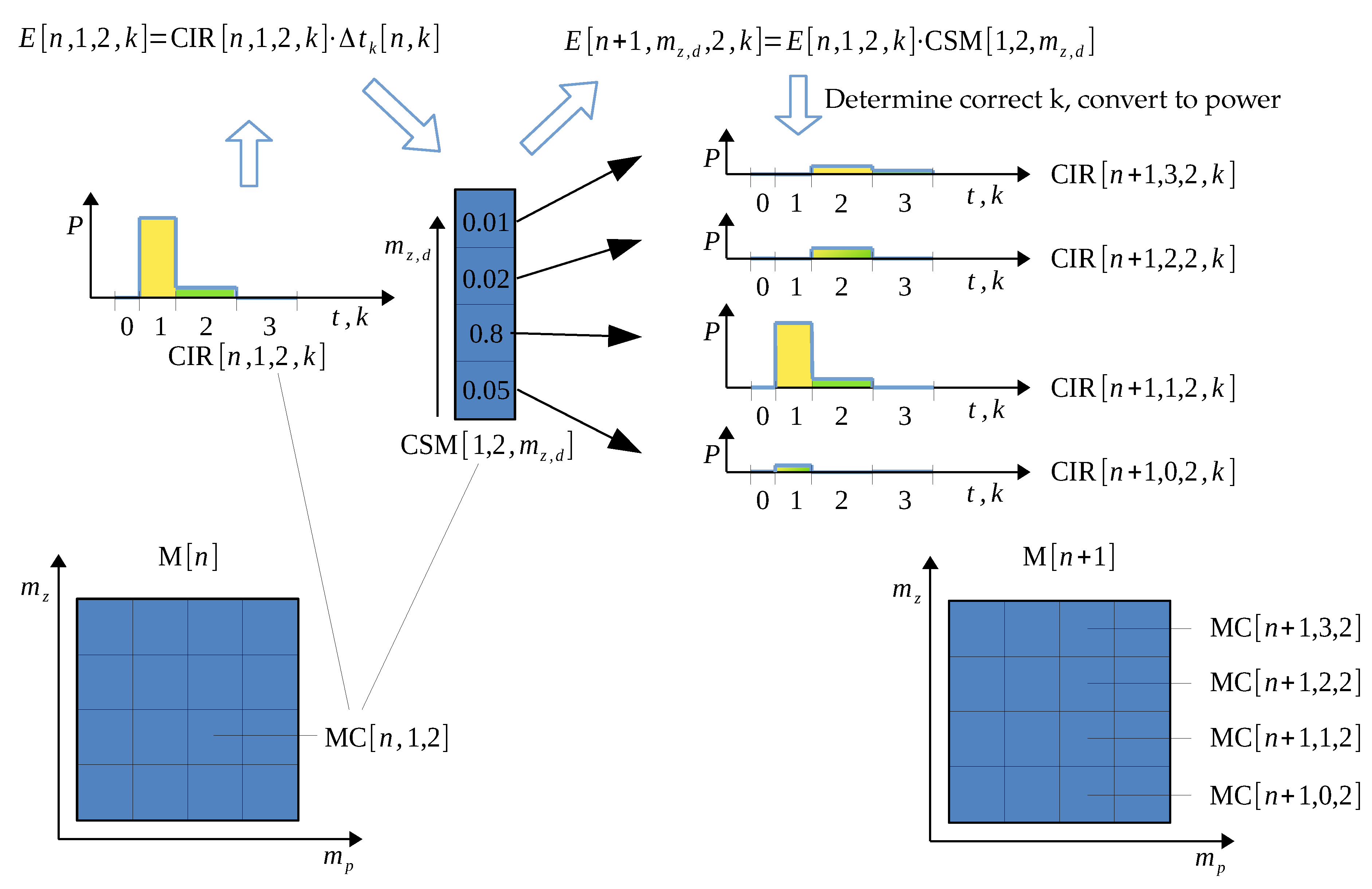
During the transition from a matrix to the next matrix , the power contained by the matrix cells of is scattered to the matrix cells of according to the scatter matrices of the originating matrix cells. Since the power of each matrix cell depends on the time and is therefore stored in a cell impulse response, the scattering process is carried out for the power of each time interval of a cell impulse response. We have discussed the determination of the arrival time of a scattered power at the destination matrix cell and the subsequent assignment of the corresponding time interval of the destination cell impulse response in the previous section. In the following, we use a simplified example to focus on the scattering process and the involved power conversions. So far, we have denoted matrix cells as . Since we discuss matrix cells of different matrices in this section, we expand the notation to to consider the position index n as well. We consider a matrix with the angular dimensions and and cell impulse responses with time intervals. As shown in Figure 7, we examine the scattering of the power contained by the time intervals of a single cell impulse response . If the example was about an ideal fiber free from scattering, would only have a power greater than 0 for , since it belongs to a matrix cell for and . Since the CIR has some power for as well, the power of this time interval must have been scattered into this CIR from a CIR with a different index during a previous matrix transition.
The first step is the derivation of the time interval energy for each time interval of which can be achieved by multiplying the power of each time interval by the corresponding temporal step width . The cell scatter matrix defines how each computed time interval energy is distributed over the destination matrix cells of the next matrix using the angular index . As of now, the model only supports scattering over which is explained in Section 2.1.4. For an ideal fiber, would have the value 1 for and 0 for all other indices. In the example, 80% of the power maintains the original angle () with only a little power being scattered to different angles. The sum of all values of is <1, which means that the total power decreases during the matrix transition due to attenuation. The next step is the calculation of the time interval energies which are scattered into particular matrix cells of the next matrix from the original time interval energy . The value of the time interval energy for each destination matrix cell can be obtained by multiplying the current time interval energy with the corresponding factor of the cell scatter matrix .
The time of arrival and subsequently the index k of the destination cell impulse response is obtained as depicted in Figure 6. The power added to the destination time interval of is computed by dividing the arriving energy by the temporal step width of the destination time interval. Due to scattering, can change during the transition, which is indicated for . In this case, power was scattered to a matrix cell with a higher . As a consequence, the index k at which the time interval energies arrive can be higher than the original index, from which the time interval energies came from. Making it easier to keep track of the index changes, the areas corresponding to the time interval energies are colored yellow (original index ) and green (original index ). The index k of the destination impulse response can also be smaller than the original index k when a time interval energy is scattered to a lower angle as it is depicted for .
Multithreading
Depending on the size of the matrices, the length of the fiber and the number of intervals of the impulse responses, the computation of the model can be demanding on both time and memory. Due to the parallel nature of the matrix cells, the model is ideally suited for multithreading. The current implementation supports up to threads. Provided a CPU with enough cores, the time necessary to compute the model can be significantly reduced. While the complete model is available as a Java implementation, the time-consuming part of the model was rewritten using the compute unified device architecture (CUDA) and integrated into the regular model. CUDA is a parallel computing platform that grants access to the graphics processing unit (GPU) of Nvidia graphics cards (Nvidia Corp., Santa Clara, CA, USA), which can offer up to a few thousand cores. While not as powerful as the cores of a regular CPU, the sheer amount of available cores makes CUDA attractive for algorithms that can be split into a large number of threads. Given that the graphics card has enough memory and depending on the regular CPU, the computation time can be further reduced.
2.1.4. Advantages and Drawbacks of the Model
The main advantage of the proposed model over existing approaches is the proper consideration of tunneling and refractive modes and their impact on the amplitude and phase response of an SI-MMF. Tunneling and refractive modes can be disabled separately in the model to investigate the impact of each mode category individually. The model can deal with light sources with arbitrary angular distributions and geometries provided their power distribution can be expressed depending on and . Equations for point sources and a two-dimensional source have already been derived [14]. Additional influences like Fresnel losses and the angular sensitivity of a given receiver can easily be considered.
A Java implementation, which was built with a focus on the modularity of the different components, exists for the model. A variety of different scenarios can be modeled and adjusted without the requirement of extensive programming skills. The implementation supports multithreading and benefits from the large number of cores of modern multicore CPUs. Working with the CUDA implementation offers the potential of an even larger performance gain, depending on the available memory and the number of cores of the GPU.
The source code of the model is open source, released under the GNU General Public License Version 3 (GPLv3) and under active development. While the features discussed in this paper are already implemented, the model is regularly expanded. Due to the licensing, everyone interested is allowed to study the code and expand it by one’s needs.
One of the drawbacks of the model is that the exact modeling of a fiber is only possible if the length is an integer multiple of . However, both amplitude and phase response change rather slowly over the length compared to , which allows good results for intermediary values by interpolation of the exact values. Another disadvantage is a consequence of the currently used scatter matrices, which were obtained from far field measurements. Even though the scatter matrices are available for all combinations of and , they only describe the power distribution over and neglect the impact on . Due to the lack of more detailed data, the model currently keeps the power distribution over constant.
2.2. Simulation of the Phase Response
We demonstrate the application of the proposed model by evaluating the impact of all influences considered by the model on an optical strain or length sensor, which is based on the phase measurement of an optical signal whose power is harmonically modulated (see Figure 3). The sensor relies on a linear relationship between the length L of a fiber and the modulation phase at the end of the fiber [10,11,16,17,18]. The requirement for this linear relation applies to every measurement technique based on phase measurements including optical frequency domain reflectometry (OFDR). The ideal phase for which this condition holds corresponds to a fiber that allows the light to propagate under the angle of only:
It can be seen that is linear to both the length of the fiber and the angular modulation frequency . However, influences like modal and chromatic dispersion, scattering, the angular power distribution of the light source and the angular receiver sensitivity influence the actual phase of the modulation at the end of the fiber. The proposed model considers all these influences when computing the impulse response of a fiber of a particular length. As described in Appendix A, the impulse response can be transferred to the frequency domain leading to the transfer function of the transmission system. The complex argument of the transfer function is the phase response which describes the modulation phase at the end of the fiber of a particular length depending on the modulation frequency. In order to evaluate the development of the modulation phase along the fiber, the model has to compute the impulse response of the fiber for each discrete position up to the maximum fiber length.
For the evaluation of the measurement error of the length sensor, which is caused by the deviation of the phase response of a particular length L from the ideal modulation phase for the same length, we use the relative error which expresses the relative deviation of a measured or simulated length from the real length L:
It is important to mention that the real phase response is neither proportional to the length L nor to angular modulation frequency . The resulting relative error is therefore not constant over or L. For demonstrative purposes, we compute the relative error of the phase based length measurement of an SI-POF with a length up to . We predict the impact of the launching condition, receiver characteristics and the modulation frequency on the relative error. Furthermore, we investigate the influence of each mode category. All simulations will be performed with the scatter and attenuation matrices obtained for an SI-POF Asahi TC-1000 (Asahi Kasei Corp., Tokyo, Japan) as described in [13]. For the refractive index and the refractive group index of the core, we use the values obtained by Beadie et al. [19] for a wavelength of : and .
2.2.1. Light Source
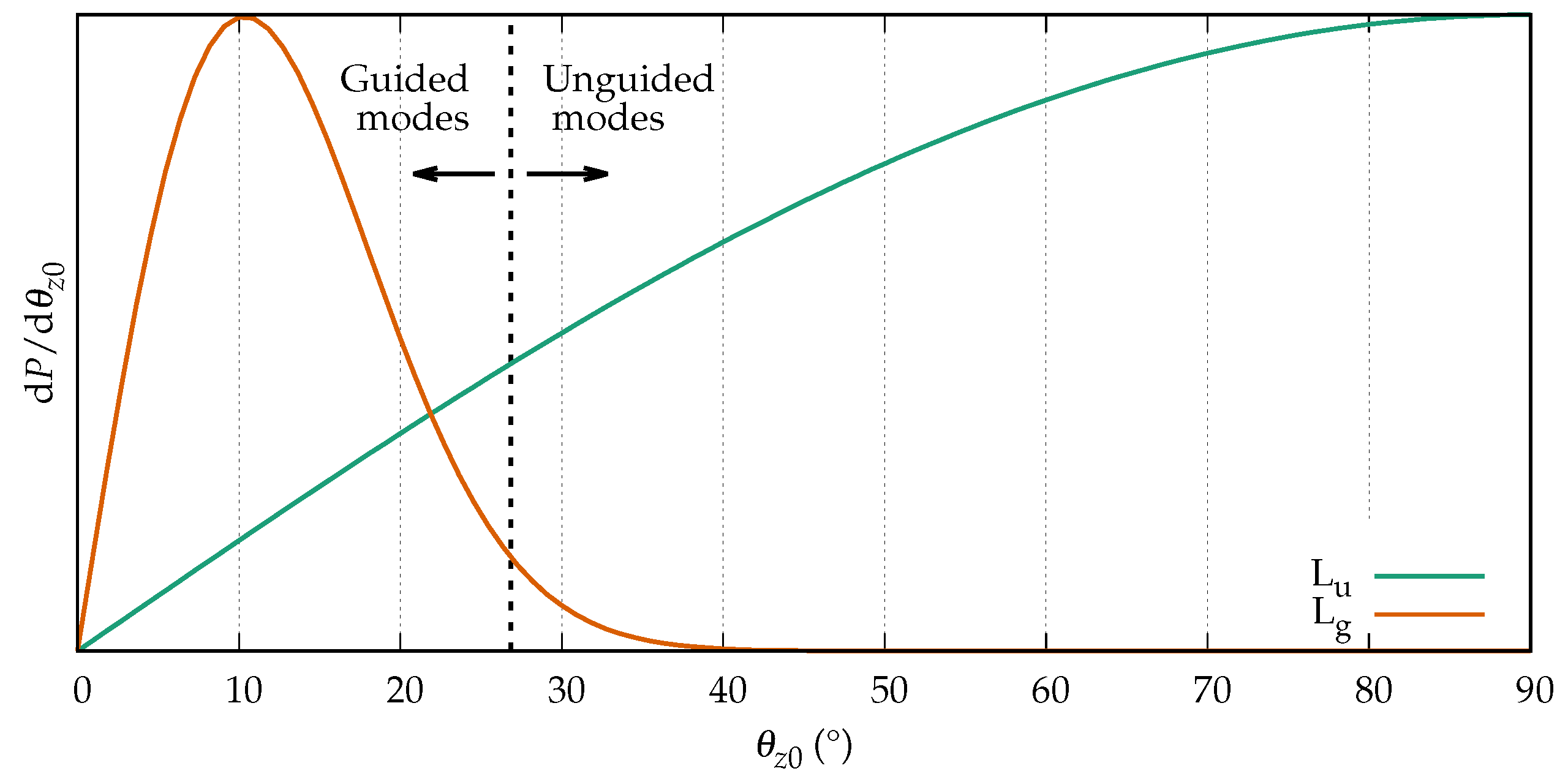
We use two different light sources for the simulations. The first one () has a uniform power distribution over a one-dimensional cross section of . Since we consider the light source to be axially symmetric around the optical axis, it has a uniform power distribution over the solid angle , which is spanned by . If is the power that would be emitted in the half space , the power P, which is emitted in the solid angle , can be expressed as
The power distribution over is
The solid angle can be expressed with respect to :
This leads to
for the derivative. The power distribution of can therefore be expressed with respect to as well:
Since we want to excite the full half space, we define a maximum angle of . Figure 8 shows the power distribution of normalized to its own maximum. While the definition of is not close to a realistic light source, it allows a uniform excitation of all possible modes, which is useful for evaluating their impact on the simulations. The source has a circular area with the same diameter as the core of the fiber and is placed right in front of the fiber. We assume that there is no gap between the light source and the front surface of the fiber. As a consequence, all rays enter the fiber at the same time. Nevertheless, we do consider Fresnel losses at the entry and the angular conversion according to Snell’s law. The power is equally distributed over the area.
The second light source has the same geometry and near field, but a non-uniform distribution over the angle and matches the angular distribution at the outputs of a Y-coupler that we used in the following experiment. The cross section of the distribution over has a Gaussian shape and can be expressed as
with . The rotational symmetric power distribution around the optical axis can be obtained by integrating over the angle around the optical axis:
The rotational symmetric power distribution of is shown in Figure 8 as well. Just like , is normalized to its own maximum in Figure 8. If we consider the maximum angle of acceptance to be
it can clearly be seen that most of the power of will excite unguided modes, whereas the majority of the power of will end up in guided modes.
2.2.2. Receiver Characteristics
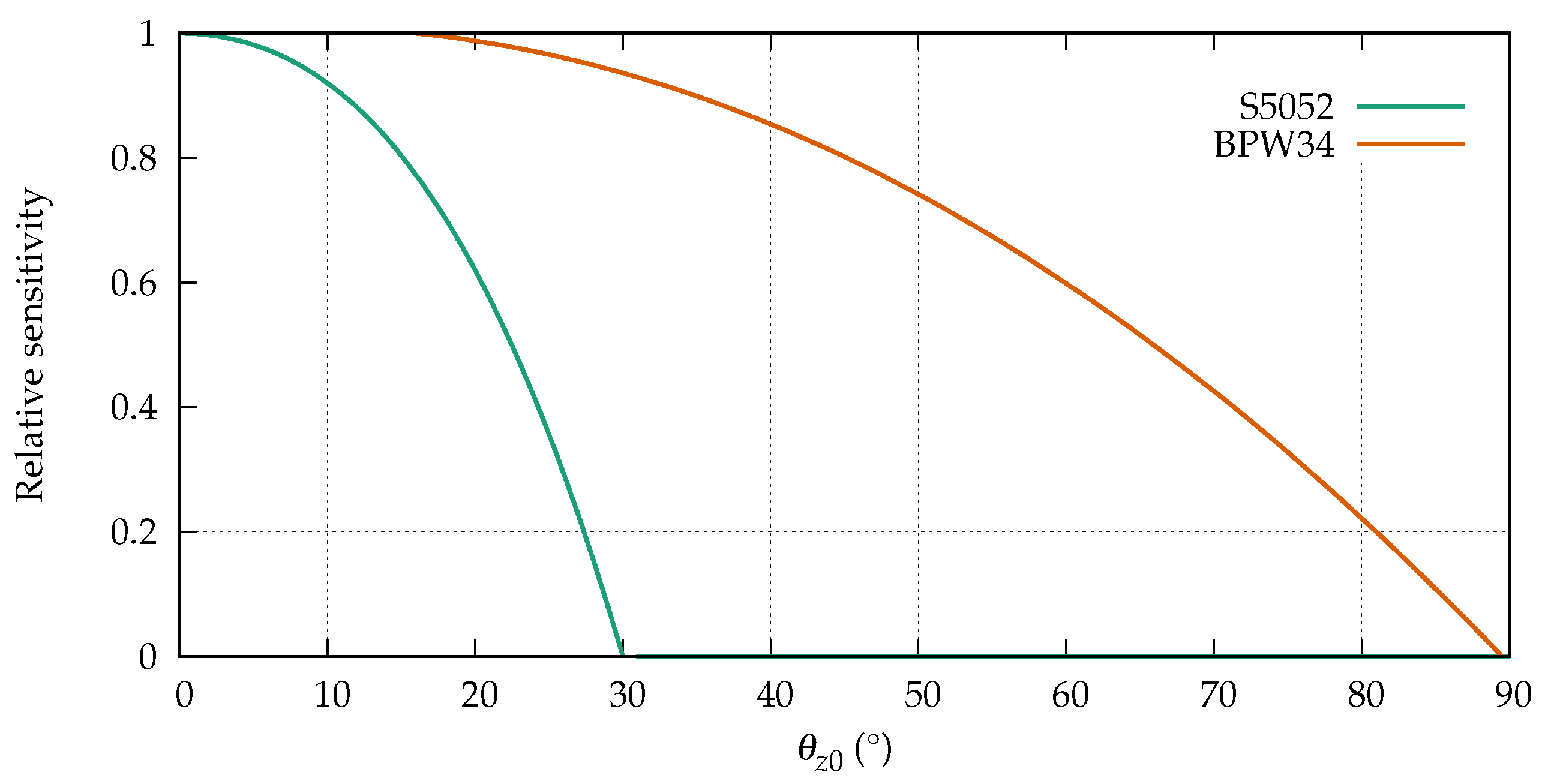
We consider two different receivers, both silicon PIN photodiodes, that will be used in the simulations and in the measurement. The first one is an S5052 [20] from Hamamatsu (Hamamatsu Photonics, Hamamatsu City, Japan) with a relatively narrow angular sensitivity. The second one is a BPW34 [21] from Vishay (Vishay Intertechnology, Inc., Malvern, PA, USA) that accepts larger angles. The angular sensitivities of both photodiodes taken from the data sheets were fitted as functions of the third order as shown in Equation (30) and are depicted in Figure 9. The corresponding coefficients are shown in Table 1:
2.2.3. Modulation Frequency of the Transmitter
Since the phase response is a function of , we will vary the frequency with which the power of the transmitter is being modulated and evaluate the impact.
2.2.4. Mode Categories
One of the features of the proposed fiber model is the inclusion of leaky modes. For the investigation of the influence of each mode category, we will perform the simulations for three different combinations:
- Guided modes,
- Guided and tunneling modes,
- Guided, tunneling and refracted modes.
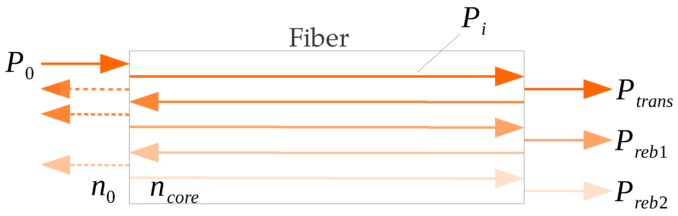
2.2.5. Influence of Reflections
Another influence on the development of the modulation phase along the fiber is optical reflection, as shown in Figure 10. When the incident light with the power enters the fiber, it is affected by Fresnel losses. The power which enters the fiber () can be expressed by the transmittance T or the reflectance R of the end surfaces of the fiber respectively:
If we assume a propagation angle of , the reflectance of the end surfaces of the fiber can be expressed as
and the transmittance as
Therefore, most of the exciting power enters the fiber and only a small part is reflected. For the same reason, the largest part of is transmitted at the end of the fiber:
However, a small part is reflected back at the end surface of the fiber. The reflected light travels back to the beginning of the fiber, is reflected again and propagates along the fiber again. The largest part of this twofold reflected light will be transmitted through the end surface, which we will call first rebound:
The first rebound superimposes the transmitted light . When the fiber is excited with a light source whose power is modulated with a fixed frequency, the first rebound can interfere with the transmitted light. It is important to mention that the interference occurs between the modulated optical powers and not between the electromagnetic fields of the light. The reflected light will travel the fiber again and lead to the second rebound
and so on. The relation between the powers of the first rebound and the transmitted light can be expressed as:
The second rebound faces four reflections:
From this consideration, one can see that the power of the second rebound is so small that its impact on the transmission behavior of a fiber is negligible. The impact of the first rebound can easily be integrated in our model by calculating a second impulse response with three times the fiber length that is attenuated by the discussed reflectivities. For the estimation of the power of the impulse rebounds, we have neglected the attenuation of the fiber. The fiber model, however, does consider absorption and scattering for the impulse rebound as well as the angular dependency of the Fresnel losses.
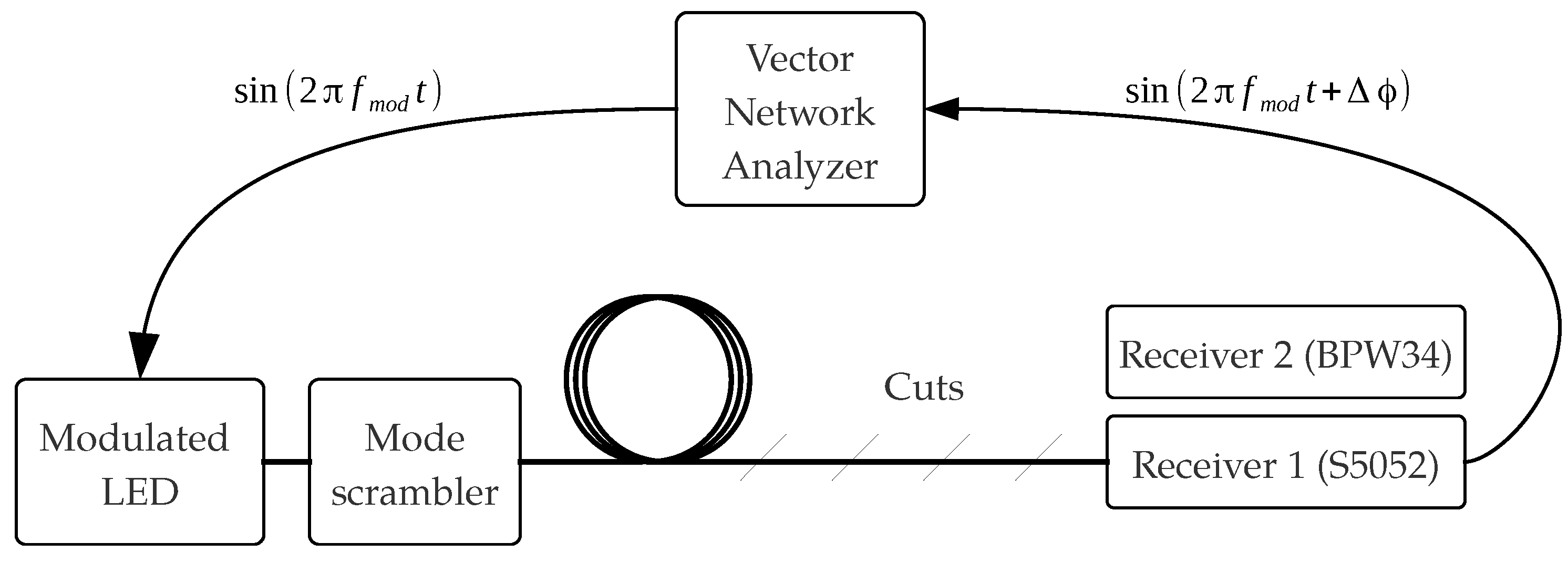
2.3. Experimental Determination of the Phase Response
To verify the results of the model, we created a cutback measurement setup which allowed us to investigate the development of the phase of a harmonically modulated signal along a fiber. This allowed us also to evaluate the error that affects a strain or length sensor that uses an SI-POF as medium. The measurement setup is depicted in Figure 11. We used the output of a vector network analyzer (VNA) to modulate the power of an LED having a wavelength of 650 with a fixed frequency. A Y-coupler acted as a mode scrambler and homogenized the slightly irregular far field of the LED, resulting in the angular power distribution of as described before at both outputs. One output was connected to the fiber under test, the other output of the Y-coupler remained unconnected. The fiber had a total length of and was coiled with a diameter of . In previous tests, the diameter had been varied between and and had been found to have a negligible impact on the development of the modulation phase. Only the last meter of the fiber was straight with a receiver attached to it. Two receivers with the described PIN photodiodes (S5052/BPW34) were used to convert the optical power into an electrical voltage which was returned to the VNA. The fiber was being cut back in 16 steps to match the step width of the model and the phase was measured with both receivers for each position. The fiber was only being cut along the straight section. When this was not possible anymore, one loop of the coiled section was unwinded. The fiber was being cut with a guided high quality blade but not polished. Polishing was avoided since it is a time-consuming process, which would have allowed the phase measurement to be affected by a possible temperature drift of the receivers. As a trade-off, the far field at the end of the fiber was affected by the relatively poor quality of the end surface which caused fluctuations in the measurement of the phase along the fiber.
The absolute modulation phase, which was measured by the receiver for each cutback step, did not only depend on the light propagation in the fiber. The electrical wiring, the transmitter and the receiver introduced a phase delay as well which influenced the measurement. Therefore, a reference measurement of the modulation phase was performed directly at the end of the mode scrambler. It was performed for each modulation frequency and for both receivers. Furthermore, the VNA could only determine the modulation phase within one modulation wavelength along the fiber. The development of the absolute phase, which was required to obtain the relative error Equation (21), was therefore reconstructed by adding up the measured phase differences between two cuts and subtracting the phase from the reference measurement.
3. Results and Discussion
3.1. Basic Validation of the Model
Before the model was used to simulate the behavior of an optical transmission system, several basic checks had been performed on the model to ensure its validity. The model offers the possibility to bypass the cell scatter matrices. In this case, the impulse response is only affected by chromatic and modal dispersion but not by attenuation and scattering. It was verified that the total energy carried by the impulse responses of the transmission system is maintained during the propagation. Furthermore, the power of each time interval k of the cell impulse response of each matrix cell is constant over the fiber length. Additionally, ray tracing simulations were set up to verify these ideal impulse responses using LightTools (version 8.4, Synopsys, Mountain View, CA, USA). The results obtained from LightTools matched the computed impulse responses of our model within the limits of accuracy given by the discrete nature of both approaches.
In order to classify the accuracy of the used scatter data, the attenuation of the Asahi TC-1000 was extrapolated from simulations performed with the model. The attenuation was found to be ≈250 dB/km, which is higher than the stated by the manufacturer [22]. However, one has to keep in mind that the used scatter data were obtained from a piece of fiber which can introduce a relatively large measurement error. Under these conditions, we consider the obtained attenuation to be in an adequate range.
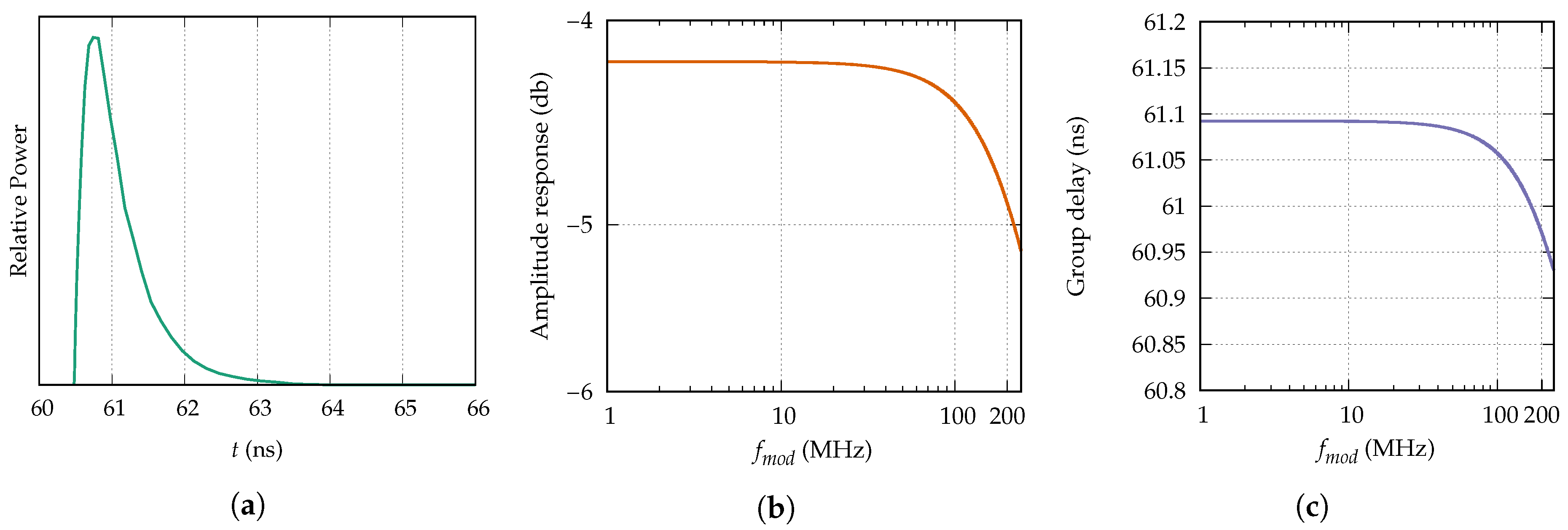
3.2. Example Simulation
For the verification of the model, we simulated the relative error of a fiber length measurement based on the phase measurement of the modulated optical power according to Equation (21). However, this required further processing of the impulse responses computed by the model. To get an impression of a simulated impulse response and the corresponding amplitude and phase response, we present the results of a example simulation in this section. Figure 12a shows an impulse response computed by the model for an SI-POF with a length of . The fiber was excited with the Gaussian power distribution and the receiver characteristics of a BPW34 photodiode were considered. Furthermore, only guided modes were excited. Figure 12b shows the corresponding amplitude response up to a maximum modulation frequency of 240 obtained by the DTFT as described in Appendix B. The computed impulse response was normalized by the energy with which the guided modes were excited. As it can be seen, the attenuation for the modulation frequency of 240 is ≈1 dB higher than for a continuous wave (CW) signal. The computed phase response is not depicted since the deviation from the ideal phase response is so small that it is not directly observable. Therefore, Figure 12c shows the group delay, which is the negative derivation of the phase response with respect to the angular modulation frequency:
As it can be seen, the group delay changes only a little within the depicted frequency range.
3.3. Results of the Simulations
We used the relative error as given by Equation (21) to determine the accuracy of the fiber length obtained from a phase measurement, when influences like modal dispersion are not considered. Therefore, the influence of impacts like modal and chromatic dispersion, the launching condition and the angular receiver sensitivity on the accuracy of a phase based length or strain sensors can be evaluated. Unless stated otherwise, all simulations were evaluated at a modulation frequency of . Since we were working with an LED, was close to the maximum achievable modulation frequency.
3.3.1. Influence of Light Source, Receiver and Mode Categories
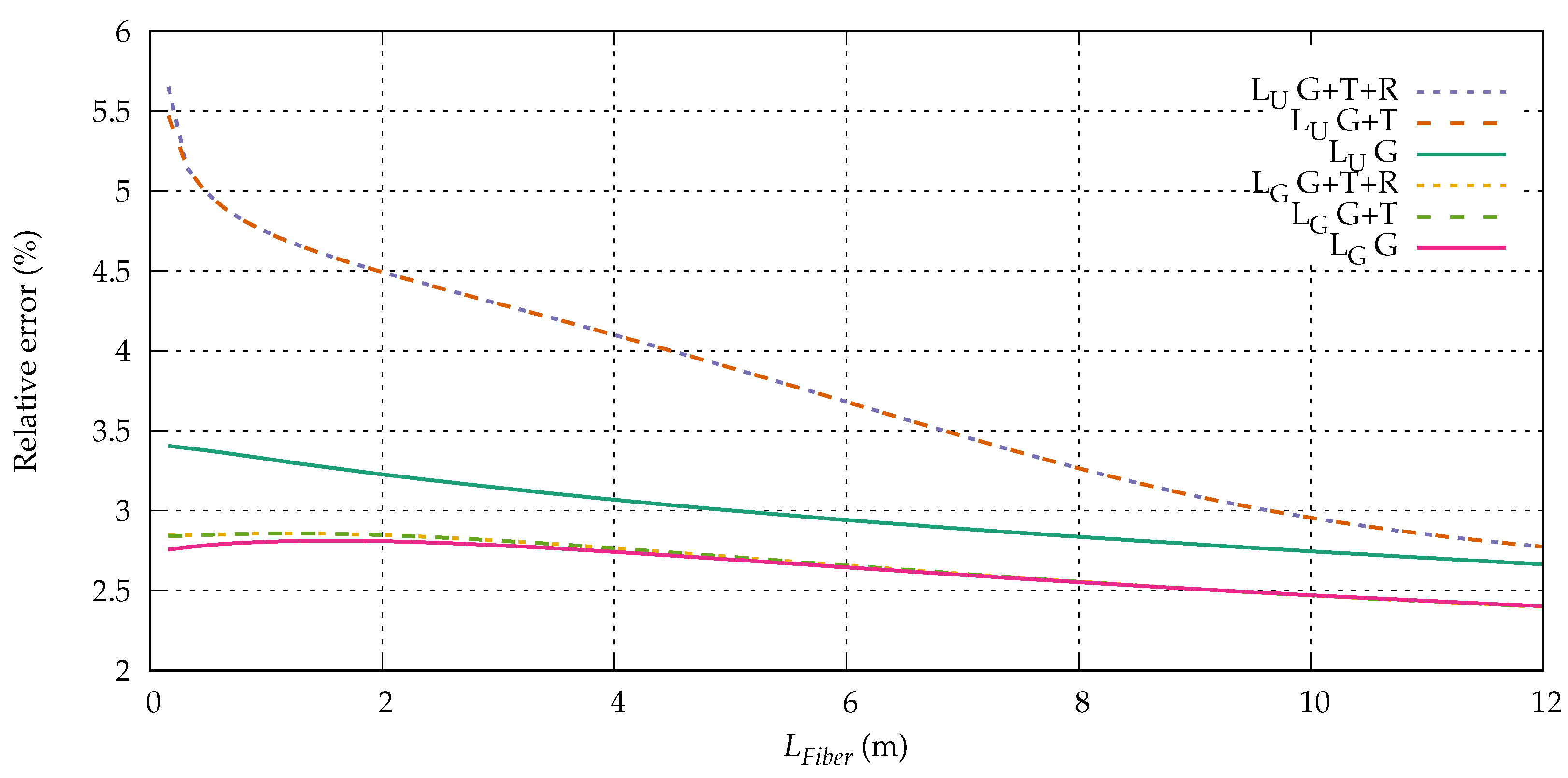
Figure 13 shows the relative error up to a length of simulated with both launching conditions (uniform distribution) and (Gaussian distribution) for the photodiode BPW34, which has a large acceptance angle. The simulation was performed with guided modes only (G), guided and tunneling modes (G + T) and finally with all possible modes including refracted modes (G + T + R). Inside the observed range, the relative error is positive in all scenarios but decreasing with the length. A positive relative error means that the measured length is longer than the real length. The light source couples more power into higher order modes than and the BPW34 detects modes up to relatively high angles (see Figure 9). Since the transit time of each ray depends on , the relative errors obtained for are larger than the ones for . If we compare the results of the three different mode categories, we can see that it does make a difference if we consider only guided modes (G) or tunneling modes additionally (G + T). The difference is more pronounced for the excitation with as for since the latter one is hardly exciting leaky rays. The further consideration of refracted modes (G + T + R) shows almost no influence on the relative error since they carry only little power, no matter which light source we choose. In fact, the influence of the refracted modes is not visible at all for the excitation with . Overall, we can see that the model predicts only small errors in the phase measurements that vary slowly with the fiber length. The optical strain or length sensor would therefore measure a strain or length that is larger than the actual strain or length. Depending on the light source, the error ranges between 2.4% and 2.8% for and 2.7% and 5.7% for .
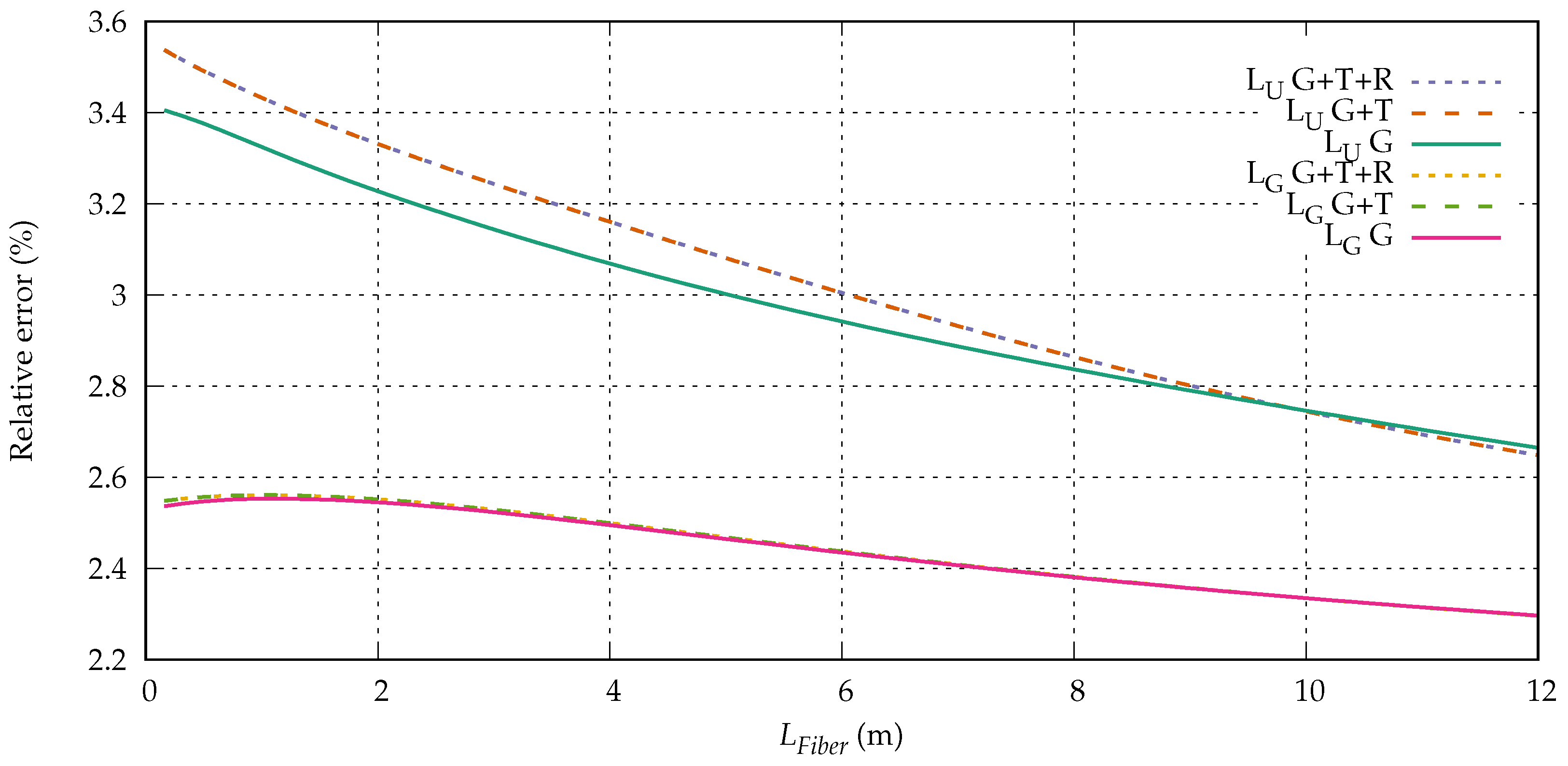
The simulations for the same conditions but for the photodiode S5052 are depicted in Figure 14. In comparison to the previous scenario, all results show a smaller relative error, which is caused by the limited angular sensitivity of this photodiode (Figure 9). The relation between the different mode categories is similar. Refracted modes play a negligible role, but this time the influence of the tunneling modes is very limited as well, since they are hardly detected by the receiver. This effect is especially pronounced for where all three mode categories can barely be distinguished, but also for the excitation with , the difference between guided and unguided modes became smaller. The error ranges between 2.3% and 2.55% for and 2.65% and 3.55% for .
It might be confusing to see that, for the excitation with , the relative error simulated for guided modes can actually get slightly larger than for the simulations that consider leaky modes as well. In the given scenario, this happens at . Since the simulation with all possible modes carries more power in higher order modes, it leads to a broader impulse response and is therefore often expected to result in a larger measurement error. However, we have to take into account that the signal is modulated with a frequency of . The phase cannot be obtained by simply considering the mean transit time of all excited modes, which would lead to a smaller relative error for the simulation of only guided modes. Instead, it is important to consider the modulation phase of each mode whose periodicity depends on its transit time and on the modulation frequency. In other words, the phase delay, which an input signal faces, does not only depend on the mean transit time of the impulse response but also on the shape of the impulse response and the modulation frequency of the input signal.
3.3.2. Influence of the Modulation Frequency
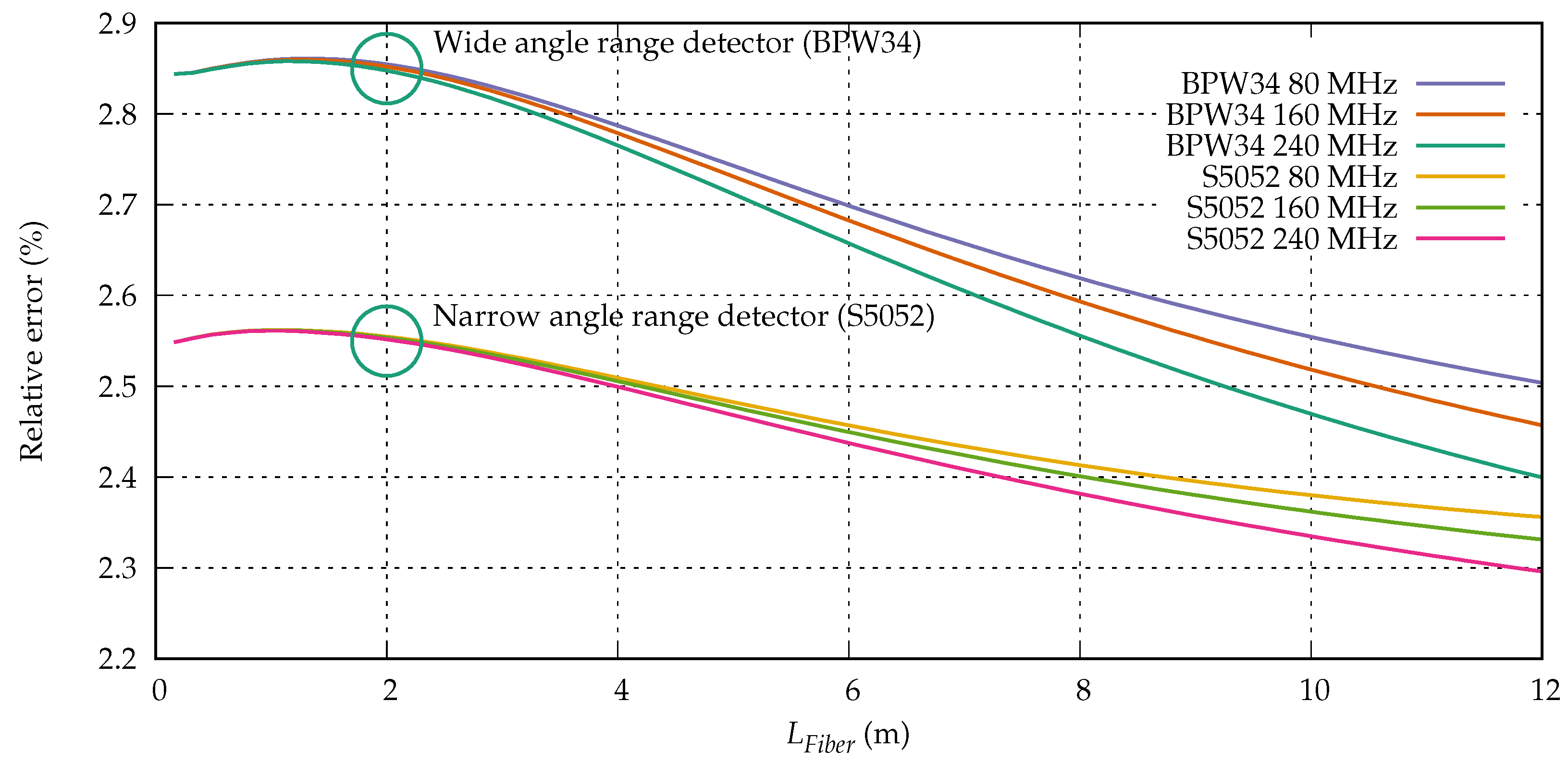
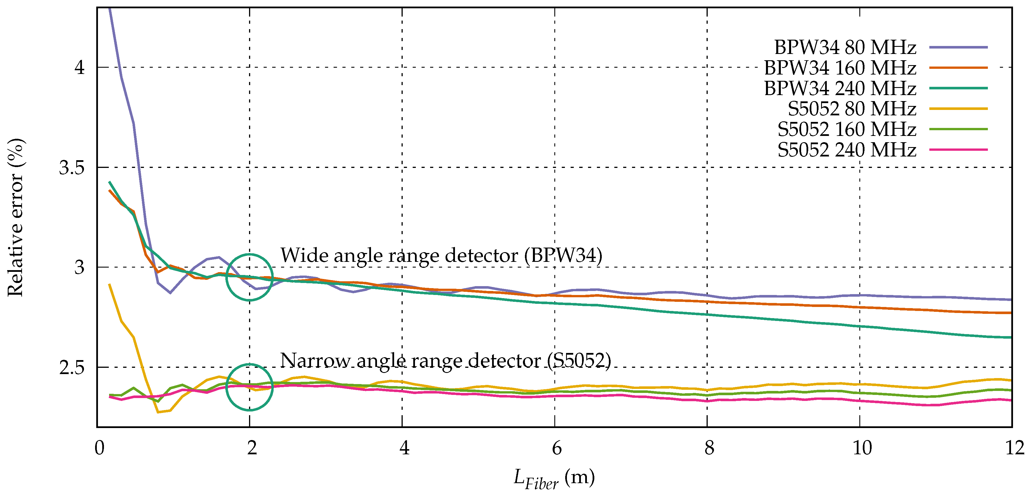
Furthermore, we evaluated the influence of the modulation frequency on the simulations. Figure 15 shows the relative error for the excitation with and both photodiodes BPW34 and S5052 for the modulation frequencies , and . The modulation frequencies were chosen from a range that could be experimentally evaluated. The simulations considered all mode categories. The relative error for was already shown in the previous diagrams. As we can see, for both photodiodes, the decrease of the relative error with the fiber length is less pronounced for lower modulation frequencies. For the BPW34, the relative error at the maximum fiber length of 12 increases from at 240 to at 80 . The effect is a little less pronounced for the S5052, where the relative error changes from (240 ) to at 80 .
3.3.3. Influence of Reflections
Figure 16 shows the same scenario but considers the first rebound as described in Section 2.2.5. For the modulation frequency of 80 , it can clearly be seen that the reflections cause an oscillating behavior of the relative error. The absolute error oscillates with a constant amplitude over the length of the fiber. Since the relative error is related to the fiber length, its amplitude has a maximum at the beginning of the fiber and decreases with the length of the fiber. The rebound has to travel two times the fiber length before it interferes with the transmitted light; therefore, the spatial oscillation period is
with being the modulation wavelength. For this leads to which can be seen in the depiction. The oscillation period for is and is harder to observe in the depiction due to the relatively large simulation step width of 16 . The oscillation at the modulation frequency of can hardly be recognized at all since the oscillation period has decreased to ≈0.42 m. For the same reason, the maximum relative error for and is less pronounced than for . Apart from the oscillations, we can see that the reflections do not influence the overall development of the relative error. For a better comparability of the different curves, we define three different errors:
- Peak error is the maximum error that occurs at the first simulated position ( ),
- Max. error is the maximum occuring error at the beginning of the fiber neglecting the peak,
- Min. error is the error at the length of 12 .
The peak error has its maximum for . The real peak value at is independent from the modulation frequency. However, since the first simulated position is and the oscillation period is shorter for higher frequencies, the peak error decreases for higher modulation frequencies.
3.4. Results of the Experiment
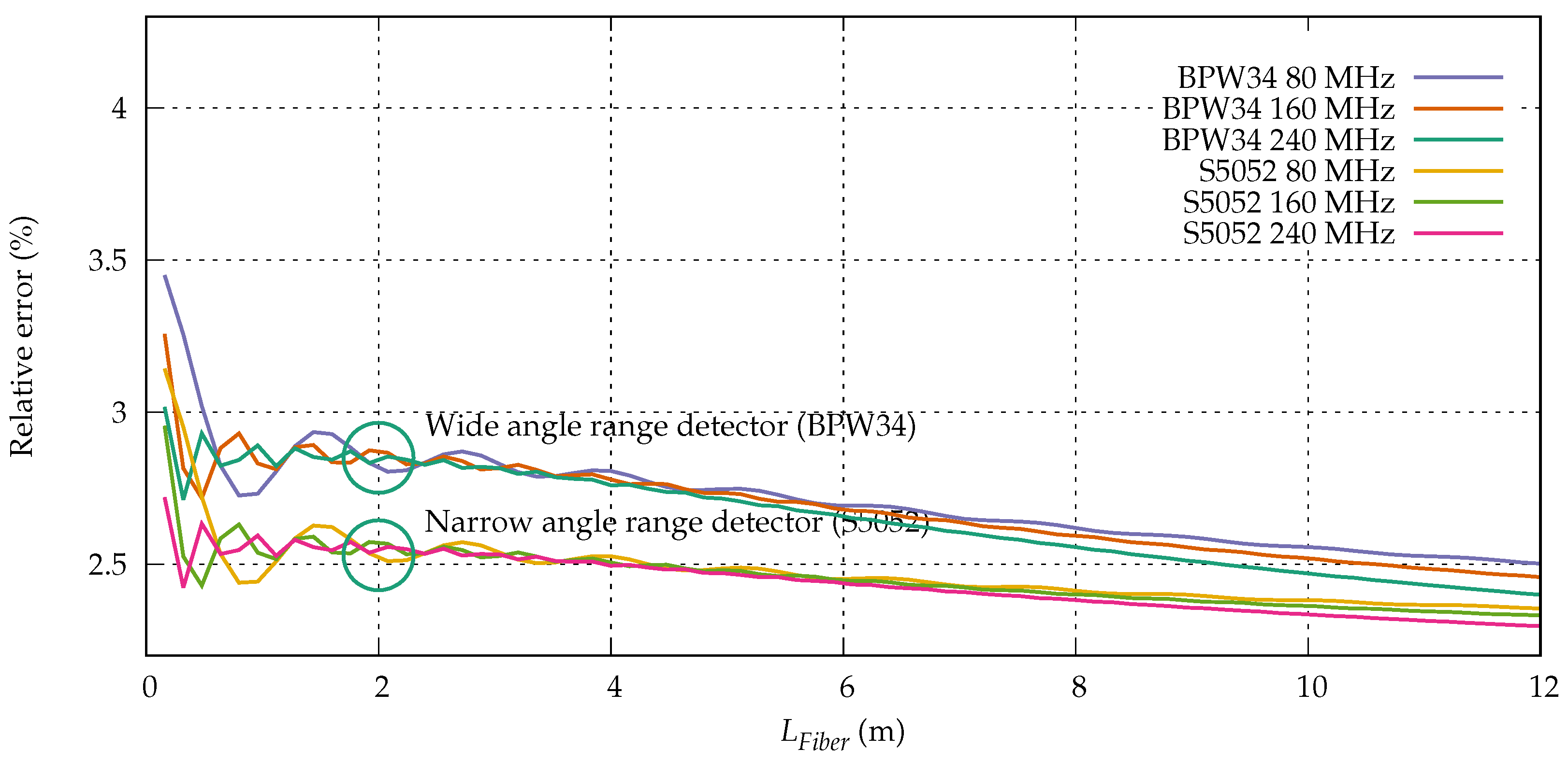
The experimental results were obtained with the measurement setup described in Section 2.3 and are shown in Figure 17. For a better comparability the depiction shows the same error range as Figure 16. Furthermore, the simulated and measured peak, maximum and minimum errors are compared in Table 2. As it can be seen, the overall development of the relative error is predicted relatively well by the model. Since the data were slightly smoothed, the oscillations for 160 and 240 are less pronounced than for the simulations. The simulated maximum error for the BPW34 is only ≈0.1% smaller than the measured maximum error. For the S5052, the predicted maximum error is ≈0.15% larger.
The reflection induced peak errors differ a little more. For the BPW34, the simulated peak error at 80 is 0.85% too small. The simulated peak errors for the other modulation frequencies are too small as well (0.15% at 160 and 0.4% at 240 ). A possible explanation is that the simulation only considers reflections at the end surfaces of the fiber. It is likely that an additional reflection occurs at the surface of the receiver, which is even stronger due to the high refractive index of silicon. The simulated peak errors for the S5052 are larger than the measured errors (0.25% at 80 , 0.6% at 160 and 0.35% at 240 ). This supports the just stated theory if we consider the fact that this photodiode has a convex lens attached to it which can reduce the amount of power that is reflected back into the fiber. Since the simulated peak errors are larger than the measured peak errors, one could conclude that the reflection at the unpolished fiber’s end surface might not be relevant at all.
The development of the relative error over the length of the fiber shows the expected dependency on the modulation frequency. The higher the frequency, the steeper the decrease of the error. In general, the decrease predicted by the model is more pronounced than for the measurements. Compared to the measurements, the minimum error predicted by the model is ≈0.35% smaller for the BPW34 and ≈0.05% smaller for the S5052. This behavior could be caused by the used scatter data, which were obtained from a 16 piece of the Asahi TC-1000. Obtaining the scatter data of such a short fiber is a complicated task since the accuracy of the results depends on a variety of different influences as described in [13]. As the decrease of the relative error happens faster in the simulation than it does in the measurement, it could be concluded that the scattering of the used data is slightly too strong.
Like in the simulation, the oscillations can best be observed at the lowest modulation frequency of 80 and their periods as well as the positions of the minima and maxima being in good agreement with the theoretical results. The curves for the S5052 are less smooth than for the BPW34, which can be explained by the smaller angular detection range. Due to the missing polishing of the end surface after each cut, the angular power distribution is partially randomized before hitting the receiver. Due to the different optical path lengths of the modes, the resulting phase depends on the sum of all detected modes. Since the receiver detects a random set of modes at each cut, the detected phase dithers within a certain range. The larger the angular detection range of the receiver, the smaller the variance of the set of detected modes. Another effect is also related to the small angular range of the S5052. Between the fiber length of 8 and 12 , the relative error varies slowly. In fact, the relative error for the S5052 increases for all frequencies between and 12 , which cannot be explained by the mode mixing at the end surface of the fiber. However, during the cutback measurement, the geometry of the fiber is altered whenever another loop is unwinded. This could have a small impact on the angular power distribution inside the fiber and therefore cause a slowly developing drift of the phase. Again, the BPW34 is not affected due to the large angular detection range.
4. Conclusions
We have presented a new propagation model for SI-MMF that enables the prediction of the transmission behavior and therefore allows the evaluation of the fiber’s behavior for both analog sensing and digital data transmission applications via the phase and amplitude response obtained from the computed impulse response. It considers the launching condition and the angular sensitivity of the receiver as well as the angle- and skewness dependent attenuation and scattering inside the fiber. The model allows the selective consideration of the different mode categories (guided, tunneling and refracted modes) to study their impact. An implementation of the model that takes full advantage of modern computer hardware is publicly available.
Simulations performed with the model lead to the conclusion that, while the influence of refracted modes on the phase response is negligible, the impact of tunneling modes depends strongly on the launching condition and on the angular sensitivity of the applied receiver. For realistic light sources, however, their impact is very limited as well.
Furthermore, we have demonstrated the application of the model by investigating the relative error that occurs in optical length or strain sensors that are based on the phase measurement of a harmonically modulated optical signal. For a fiber up to a length of 12 , the resulting length measurement error lies in the range of 2% to 3%, if the discussed influences like modal dispersion or the refractive group index are not properly considered, and changes only slowly with the length of the fiber as long as reflections are neglected. They can, however, be covered by the model as well by adding a second impulse response that is caused by the reflections. The determination of the proper reflectivities is, however, a demanding task since the reflectivity of the photodiode has to be taken into account as well.
A cutback measurement has been performed with different receivers and modulation frequencies to verify the model. The results are generally in good agreement with the simulations and the deviations can be explained. If we neglect reflections, the maximum deviation of the relative error of the measurement from the model occurs for the minimum error of the BPW34 at , where the measured error is ≈0.35% larger than predicted. While receivers with a broader angular acceptance range show a larger overall error, they are less prone to fluctuations of the modal power distribution caused by unprepared end surfaces or the geometry of the fiber.
Supplementary Materials
An implementation of the presented fiber model is included in the open source project POFToolBox, which is available at: https://github.com/POF-AC/POFToolBox.
Author Contributions
T.B. wrote the paper and is responsible for the theoretical work and the development of the fiber model. In addition, he designed and performed the experiments and analyzed the obtained data. B.S. and R.E. were involved in the design of the experiments and provided support during the development of the fiber model.
Funding
The work was supported by the European Union by means of the European Regional Development Fund (No. EU-1607-0017, Europäischer Fonds für regionale Entwicklung, EFRE).
Acknowledgments
The authors gratefully acknowledge the support of the graduate study group Fiber Optic Transmission and Sensing (FiTS).
Conflicts of Interest
The authors declare no conflict of interest.
Abbreviations
The following abbreviations are used in this manuscript:
| CP | Cell Power |
| CIR | Cell Impulse Response |
| CSM | Cell Scatter Matrix |
| CUDA | Compute Unified Device Architecture |
| DTFT | Discrete-Time Fourier Transform |
| GOF | Glass Optical Fiber |
| GPLv3 | GNU General Public License Version 3 |
| GPU | Graphics Processing Unit |
| M | Matrix |
| MC | Matrix Cell |
| MMF | Multi-Mode Fiber |
| OFDR | Optical Frequency Domain Reflectometry |
| PFE | Power Flow Equation |
| POF | Polymer Optical Fiber |
| SI-MMF | Step-Index Multi-Mode Fiber |
| SI-POF | Step-Index Polymer Optical Fiber |
| SMF | Single-Mode Fiber |
| VNA | Vector Network Analyzer |
Appendix A. Optical Transmission System in Time and Frequency Domain
Appendix A.1. Continuous Time Domain
Linear, time-invariant optical transmission systems can be described by their impulse response , which is by definition the response of the system to the excitation with a Dirac-impulse . describes how the time-dependent input signal is transferred to the time-dependent output signal by convolution:
The convolution of the two signals and can be expressed as
From Equation (A2), it is clear that the dimensions of have to be time if is supposed to have the same dimensions as . Since the proposed model is based on the optical power, the dimension of the input and output signal is power in both time and frequency domain.
For the derivation of the impulse response of the optical transmission system, we excite the system with an optical Dirac-impulse , which has the dimension power:
with being the total energy of :
Just like , has the dimension time as well. We assume a continuous impulse response of the system obtained from the model, which has the dimension power. In order to get the required dimension time, the obtained impulse response has to be normalized to the total exciting energy :
When is transferred to the frequency domain by a Fourier transform, the resulting frequency response is the angular modulation frequency-dependent complex transfer function of the transmission system:
which transfers the complex input signal to the complex output signal :
is the angular modulation frequency of the optical input power, and are the complex counterparts in the frequency domain of and in the time domain:
and include the amplitude and phase of the power modulation. The suitability of the transmission system for specific applications can be evaluated by extracting the amplitude and phase response ( and ) from the complex transfer function:
The amplitude response describes how the amplitude of an input signal of a specific modulation frequency is affected by the transmission. The phase response expresses how the modulation phase of the input signal is delayed by the transmission.
Appendix A.2. Discrete Time Domain
So far, we have discussed the processing of a continuous impulse response . Due to the discrete nature of the proposed model, we have to consider a time-discrete response with the time index k. When transferred to the frequency domain using the discrete-time Fourier transform (DTFT), which is suitable for aperiodic time signals, the resulting frequency response is continuous over the modulation frequency and can be evaluated at arbitrary modulation frequencies. However, an important difference arises when working with discrete instead of continuous impulse responses. The discrete output signal can be obtained by the discrete convolution of the discrete impulse response and the discrete input signal :
Since is supposed to have the same dimensions as , has to be dimensionless. This is an important difference to , whose dimension has to be time as we have seen in the previous section. In order to obtain the normalized discrete impulse response from the discrete impulse response calculated by the model, has to be multiplied with the temporal step width of the interval before the normalization:
Appendix B. Discrete Time Fourier Transformation for Unevenly Sampled Time Signals
The DTFT for evenly sampled data is defined as
is the equidistant input signal in the time domain with the time index k, is the temporal step width and is the resulting continuous signal in the frequency domain depending on the angular modulation frequency . Since we exclusively consider non-periodic time signals, the DTFT can be adjusted to non equidistant time signals by replacing the term by the actual time which corresponds to the interval k. The DTFT can then be expressed as
The boundaries of the DTFT are set to and ∞ since it is defined for aperiodic signals. We will adjust the boundaries to the ones of the impulse responses computed by the model. By definition, the DTFT considers to be 0 outside of these boundaries. Furthermore, the consideration of the interval-dependent temporal step width is necessary when deriving the normalized impulse response . Analogous to Equation (A13), we can write
with being the real temporal step width of each interval as explained in Cell Impulse Response.
References
- Gloge, D. Optical Power Flow in Multimode Fibers. Bell Syst. Tech. J. 1972, 51, 1767–1783. [Google Scholar] [CrossRef]
- Gloge, D. Impulse Response of Clad Optical Multimode Fibers. Bell Syst. Tech. J. 1973, 52, 801–816. [Google Scholar] [CrossRef]
- Marcuse, D. Theory of Dielectric Optical Waveguides; Academic Press: Cambridge, MA, USA, 2012. [Google Scholar]
- Saleh, B.E.A.; Abdula, R.M. Optical interference and pulse propagation in multimode fibers. Fiber Integr. Opt. 1985, 5, 161–201. [Google Scholar] [CrossRef]
- Gasulla, I.; Capmany, J. Transfer function of multimode fiber links using an electric field propagation model: Application to Radio over Fibre Systems. Opt. Express 2006, 14, 9051. [Google Scholar] [CrossRef] [PubMed]
- Zubia, J.; Arrue, J. Plastic Optical Fibers: An Introduction to Their Technological Processes and Applications. Opt. Fiber Technol. 2001, 7, 101–140. [Google Scholar] [CrossRef]
- Yabre, G. Comprehensive theory of dispersion in graded-index optical fibers. J. Lightwave Technol. 2000, 18, 166–177. [Google Scholar] [CrossRef] [Green Version]
- Zubia, J.; Durana, G.; Aldabaldetreku, G.; Arrue, J.; Losada, M.; Lopez-Higuera, M. New method to calculate mode conversion coefficients in si multimode optical fibers. J. Lightwave Technol. 2003, 21, 776–781. [Google Scholar] [CrossRef]
- Snyder, A.W.; Love, J.D. Optical Waveguide Theory; Springer: Berlin, Germany, 2000. [Google Scholar]
- Diez, J.; Luber, M.; Poisel, H.; Ziemann, O. Stretching Sensor Based on Polymer Optical Fibers. In Proceedings of the Optical Sensors 2010, Karlsruhe, Germany, 21–24 June 2010. [Google Scholar] [CrossRef]
- Durana, G.; Kirchhof, M.; Luber, M.; de Ocariz, I.S.; Poisel, H.; Zubia, J.; Vazquez, C. Use of a Novel Fiber Optical Strain Sensor for Monitoring the Vertical Deflection of an Aircraft Flap. IEEE Sens. J. 2009, 9, 1219–1225. [Google Scholar] [CrossRef] [Green Version]
- Becker, T.; Ziemann, O.; Engelbrecht, R.; Schmauss, B. Optical Strain Measurement with Step-Index Polymer Optical Fiber Based on the Phase Measurement of an Intensity-Modulated Signal. Sensors 2018, 18, 2319. [Google Scholar] [CrossRef] [PubMed]
- Becker, T.; Schmauss, B.; Gehrke, M.; Nkiwane, E.; Engelbrecht, R.; Ziemann, O. Angle and Skewness dependent Scattering and Attenuation Measurement of Step-Index Polymer Optical Fibers. In Proceedings of the 26th International Conference on Plastic Optical Fibers, Aveiro, Portugal, 13–15 September 2017. [Google Scholar]
- Becker, T.; Schmauss, B.; Gehrke, M.; Nkiwane, E.; Ziemann, O. Analytical model for the angle-dependent power distribution in optical multimode fibers. In Proceedings of the 25th International Conference on Plastic Optical Fibers, Birmingham, UK, 13–16 September 2016. [Google Scholar]
- Becker, T. POFToolBox. Toolset for Modeling the Transmission Behavior of SI-POF. Available online: https://github.com/POF-AC/POFToolBox (accessed on 27 March 2018).
- Silva-López, M.; Fender, A.; MacPherson, W.N.; Barton, J.S.; Jones, J.D.; Zhao, D.; Dobb, H.; Webb, D.J.; Zhang, L.; Bennion, I. Strain and temperature sensitivity of a single-mode polymer optical fiber. Opt. Lett. 2005, 30, 3129–3131. [Google Scholar] [CrossRef] [PubMed] [Green Version]
- Kiesel, S.; Peters, K.; Hassan, T.; Kowalsky, M. Single-Mode Polymer Optical Fiber Sensors for High-Strain Applications. In Proceedings of the 19th International Conference on Optical Fibre Sensors, Perth, WA, Australia, 14–18 April 2008. [Google Scholar] [CrossRef]
- Kiesel, S.; Peters, K.; Hassan, T.; Kowalsky, M. Behaviour of intrinsic polymer optical fibre sensor for large-strain applications. Meas. Sci. Technol. 2007, 18, 3144–3154. [Google Scholar] [CrossRef]
- Beadie, G.; Brindza, M.; Flynn, R.A.; Rosenberg, A.; Shirk, J.S. Refractive index measurements of poly(methyl methacrylate) (PMMA) from 0.4–1.6 μm. Appl. Opt. 2015, 54, F139. [Google Scholar] [CrossRef] [PubMed]
- Hamamatsu Corporation. Si PIN Photodiode S7797, S5052, S8255, S5573. Available online: http://www.htmldatasheet.com/hamamatsu/s5052.htm (accessed on 22 March 2018).
- Vishay Semiconductors. Silicon PIN Photodiode BPW34, BPW34S. Available online: https://www.vishay.com/docs/81521/bpw34.pdf (accessed on 22 March 2018).
- Asahi Kasei Corporation Products–Bare Fibers. Available online: http://www.asahi-kasei.co.jp/ake-mate/pof/en/product/data-communication.html (accessed on 1 March 2018).
Figure 1.
Meridional and skew modes of the same differ by their optical path (a) and their skewness (b).
Figure 1.
Meridional and skew modes of the same differ by their optical path (a) and their skewness (b).

Figure 2.
Mode categories of a step-index multi-mode fiber (SI-MMF).

Figure 3.
Change of the modulation phase due to strain.

Figure 4.
Schematic overview of the model.

Figure 5.
Covering the front surface of a fiber (a) to influence the possible range (b).

Figure 6.
Cell impulse responses of the model.

Figure 7.
Transition of a cell impulse response to the next matrix.

Figure 8.
Normalized power distributions of the light sources.

Figure 9.
Angular receiver sensitivities.

Figure 10.
Reflections in the fiber.

Figure 11.
Measurement setup.

Figure 12.
Simulated impulse response (a), amplitude response (b) and group delay (c).

Figure 13.
Simulated relative error considering the BPW34.

Figure 14.
Simulated relative error considering the S5052.

Figure 15.
Simulated relative error considering different modulation frequencies.

Figure 16.
Simulated relative error considering reflections.

Figure 17.
Relative error of the fiber length obtained from the measured phase.


Table 1.
Parameters of the angular receiver sensitivity.
| Receiver | a () | b () | c () | d | |
| S5052 | 1 | 30 | |||
| BPW34 | 0 | 1 | 90 |
Table 2.
Measured and simulated relative error.
| Receiver | Modulation Frequency | Peak Error Measured/Simulated | Max. Error Measured/Simulated | Min. Error Measured/Simulated |
|---|---|---|---|---|
| BPW34 | 80 | 4.3%/3.45% | 2.95%/2.85% | 2.85%/2.5% |
| BPW34 | 160 | 3.4%/3.25% | 2.95%/2.85% | 2.8%/2.45% |
| BPW34 | 240 | 3.4%/3.0% | 2.95%/2.85% | 2.65%/2.4% |
| S5052 | 80 | 2.9%/3.15% | 2.4%/2.55% | 2.45%/2.35% |
| S5052 | 160 | 2.35%/2.95% | 2.4%/2.55% | 2.4%/2.35% |
| S5052 | 240 | 2.35%/2.7% | 2.4%/2.55% | 2.35%/2.3% |
© 2018 by the authors. Licensee MDPI, Basel, Switzerland. This article is an open access article distributed under the terms and conditions of the Creative Commons Attribution (CC BY) license (http://creativecommons.org/licenses/by/4.0/).
Share and Cite
MDPI and ACS Style
Becker, T.; Engelbrecht, R.; Schmauss, B. Novel Model for the Angle and Skewness Dependent Transmission Behavior of Step-Index Polymer Optical Fiber. Fibers 2018, 6, 65. https://0-doi-org.brum.beds.ac.uk/10.3390/fib6030065
AMA Style
Becker T, Engelbrecht R, Schmauss B. Novel Model for the Angle and Skewness Dependent Transmission Behavior of Step-Index Polymer Optical Fiber. Fibers. 2018; 6(3):65. https://0-doi-org.brum.beds.ac.uk/10.3390/fib6030065
Chicago/Turabian StyleBecker, Thomas, Rainer Engelbrecht, and Bernhard Schmauss. 2018. "Novel Model for the Angle and Skewness Dependent Transmission Behavior of Step-Index Polymer Optical Fiber" Fibers 6, no. 3: 65. https://0-doi-org.brum.beds.ac.uk/10.3390/fib6030065
Note that from the first issue of 2016, this journal uses article numbers instead of page numbers. See further details here.