Article

Statistical Analysis of Mechanical Stressing in Short Fiber Reinforced Composites by Means of Statistical and Representative Volume Elements

Leibniz-Institut für Polymerforschung Dresden e.V. (IPF), Hohe Straße 6, 01069 Dresden, Germany
*
Author to whom correspondence should be addressed.
Submission received: 6 February 2021 / Revised: 24 February 2021 / Accepted: 26 April 2021 / Published: 6 May 2021
(This article belongs to the Special Issue Simulation of Short-Fiber-Reinforced Polymers)

Abstract

:
Analyzing representative volume elements with the finite element method is one method to calculate the local stress at the microscale of short fiber reinforced plastics. It can be shown with Monte-Carlo simulations that the stress distribution depends on the local arrangement of the fibers and is therefore unique for each fiber constellation. In this contribution the stress distribution and the effective composite properties are examined as a function of the considered volume of the representative volume elements. Moreover, the influence of locally varying fiber volume fraction is examined, using statistical volume elements. The results show that the average stress probability distribution is independent of the number of fibers and independent of local fluctuation of the fiber volume fraction. Furthermore, it is derived from the stress distributions that the statistical deviation of the effective composite properties should not be neglected in the case of injection molded components. A finite element analysis indicates that the macroscopic stresses and strains on component level are significantly influenced by local, statistical fluctuation of the composite properties.

Graphical Abstract

1. Introduction

For an accurate numerical design of a component made of short fiber reinforced plastics, knowledge of the local and especially the fiber orientation-dependent effective composite properties are necessary. Several modelling techniques are discussed in the known literature. Besides the Meanfield approaches [1,2,3,4], which are based on the work of Eshelby [5], the Fullfield analysis of the composite is also known [6,7,8,9,10,11,12,13,14]. In this method a certain volume of the composite is modelled and usually numerically analyzed. The modelling includes the geometric representation of the composite, the use of appropriate constitutive equations for the individual phases of the composite and the application of suitable boundary conditions. The resulting boundary value problem can then be solved with various methods, for example with the finite element method (FEM) [6] or a Fast Fourier approach [15].
In the literature, the influences of different modelling of the finite volume on the effective composite properties can be found [16,17,18,19,20,21,22,23,24,25,26,27]. This includes the definition of the finite volume itself, which is usually referred to as a Representative Volume Element (RVE). Different approaches for RVEs have been discussed so far. Hill [12] coined the term RVE. By his definition, an RVE is a section of a composite that must be statistically representative of the entire composite. Additionally, he demands a sufficiently high number of inclusions to neglect boundary effects. Another definition of the term RVE is provided by Drugan and Willis [13]. They define a RVE as the smallest volume that can be used to calculate an effective average of a composite property. Using two-dimensional RVEs with circular inclusions, Gitman et al. [14] work out the existence or non-existence of RVEs depending on the constitutive equations used and the influence of size and periodicity on the effective composite properties. Moreover, it is known that each (different) realization of a RVE can provide a different value of the effective composite properties, so that a statistical consideration must be made, for which Monte-Carlo simulations are particularly suitable [9]. It has been shown that an effective mean value can be calculated over several small RVEs instead of one large one [28,29,30]. Thereby, the probability of a large deviation from the mean value is less for larger volumes. Accordingly, the Hill and the Drugan and Willis approaches must provide the same mean value but a different standard deviation of the effective composite properties.
The question that arises from this is whether such a standard deviation has a physical significance for applications of short fiber reinforced plastics and must be computed correctly or whether it can be neglected. To answer this research question, this paper calculates the standard deviation of the effective composite stiffness of a short fiber reinforced plastic as a function of the volume under consideration. Therefore, two different approaches for the definition of the finite volume are used. This is followed by a subsequent critical evaluation, especially against the background of a locally different fiber orientation of real components. This is accomplished with a finite element analysis (FEA) at the macroscopic component level, considering the local distribution of composite properties.

2. Materials and Methods

The standard deviation of the effective composite stiffness of a short fiber reinforced plastic is calculated by running a Monte-Carlo simulation of RVEs. The modelling and subsequent homogenization for the calculation of the effective composite properties is largely taken from a previous study [25] and briefly presented in the following.
The microstructure investigated in this paper is defined by a fiber geometry, a fiber lengths distribution (LDF), a fiber volume fraction, a fiber orientation distribution (ODF), a fiber arrangement and the phase properties. For a realization of the microstructure within the Monte-Carlo simulation it is first necessary to determine how many fibers are used. The length l of the fibers is defined according to a given fiber length distribution. Analogously, the spatial orientation of the fibers is defined based on a fiber orientation density function. The volume of the matrix phase is determined in relation to the realized fibers and the prescribed fiber volume fraction. Subsequently, the fibers are randomly placed in the volume so that the microstructure is periodic and none of the fibers are overlapping with each other. The described procedure for the creation of a fiber ensemble is illustrated in Figure 1.
In addition to the procedure described above, another variant is also examined in this paper. Here, the volume is not determined based on the defined fibers but based on the total fiber length distribution and fiber orientation. In each realization the total volume is therefore constant. Thus, the fiber volume fraction for a single realization allows a deviation, but on average over many realizations the fiber volume fraction equals the defined value. In the following, this variant will be referred to as Statistical Volume Element (SVE), while the variant with the constant fiber volume fraction will be referred to as Representative Volume Element (RVE).
It is assumed that the mean value of the effective composite properties, calculated from many realizations, is identical for both variants. This assumption is to be checked by the findings of this study. However, the standard deviation should be different depending on the size of the finite volume.
Figure 2 further illustrates the difference between the SVE and RVE approach. For this purpose, a composite is shown in a two-dimensional way. The SVE approach can be interpreted as a section of constant size, where the fiber volume content v F can vary accordingly. The RVE, on the other hand, must be adjusted in size to maintain the same fiber volume content. Table 1 summarizes the different definitions of SVE and RVE.
In this paper, the effective stiffness of the composite in the fiber direction is investigated. For this purpose, the local stress fields for an applied periodic displacement are calculated by the FEM using the commercial software ABAQUS from DASSAULT SYSTEMS. Since in this study the resulting volume averaged stress σ ^ r is uniaxial, the effective stiffness E ^ r of a fiber ensemble r is determined by
E ^ r = σ ^ r ε ^ r ,
with the volume averaged strain ε ^ r . Note that, for simplicity, the directional indexing of the tensorial variables is not shown. Stresses and strains used are in the direction of the applied displacement. For the exact application of the periodic displacement boundary conditions in a non-periodic network, as well as the exact procedure of homogenization, reference is made to a previous investigation [25]. Figure 3 summarizes the calculation of the effective stiffness with a Monte-Carlo simulation. First, a microstructure is realized and the local stress and strain fields are determined by means of a FEA. Consequently, the volume averaged stress and strain is calculated by homogenization. From this the effective stiffness of the individual realization can be derived. This procedure is repeated n-times with further fiber ensembles.
The investigation in this paper is performed using a polybutylene terephthalate based (PBT) composite with 20.0 percent by weight (11.6 percent by volume) of glass fibers (PBT-GF20). The composite material is of type 2300 GV1/20 from Celanex [31]. In this section, a mechanical characterization of the composite and the non-reinforced matrix material is given. The characterization is performed from test specimens cut out of 2 mm thick injection-molded plates (90 mm × 90 mm × 2 mm). The shape of the test specimen corresponds to DIN EN ISO 527 1BA. The injection-molded plates and the orientation of the specimens on the plates are shown in Figure 4. Furthermore, the used coordination system is given. The specimens are prepared in such a way that the tensile direction corresponds to the flow direction of the injection molding process. This direction is labelled as 2-direction, the 1-direction is perpendicular to the flow direction and the 3-direction points in the thickness direction of the plate. Moreover, Figure 4 shows the true stress and strain of the experimental tests. Shown are the mean value and the standard deviation of 5 repetitions of the measurement. Furthermore, a fit of linear–elastic material models to the mean value of the characterization tests is shown, as used in the simulations. At approx. 35 MPa and 45 MPa, respectively, a substantial deviation of the measured stress curves from the linear model can be recognized. As a second parameter for the isotropic, linear–elastic material model, the poisons ratio is taken from [32]. Values for the glass fibers, which are also modelled as isotropic, linear–elastic material, are taken from [32,33]. The used parameters are shown in Table 2.
Microcomputed tomography (µCT) can be used to determine the fiber orientation of short fiber reinforced plastics. Therefore, a cylindrical specimen with a diameter of 2 mm is taken from the center of a plate. The specimen is examined with a resolution of 1.80 μm voxel edge length and evaluated in 20 equidistant slices. For each slice, the fiber orientation tensor of second order a determined by
a = a i j = 1 k N Δ z k · r k 2 · k N Δ z k · r k 2 · ( n k ) i · ( n k ) j
where Δ z k is the length, Δ r k the radius and n k is the direction of a fiber k . Figure 5 shows the components of the experimentally determined fiber orientation tensor a over the thickness of the injection molded PBT-GF20 plates.
According to Figure 5, the fiber orientation can be divided into two outer boundary layers and one middle layer. The middle layer can be identified between 0.9 mm and 1.2 mm. In the boundary layers the largest value of the fiber orientation tensor is a 22 , in the middle layer it is a 11 .
The ODF is reconstructed by the method of maximum entropy [34] from the averaged fiber orientation tensor of the boundary layers, neglecting the core layer between 0.9 mm and 1.2 mm. Figure 6 shows the procedure with the used fiber orientation tensor a and the resulting ODF. The color of the ODF shows the probability that a fiber points in this specific direction.
The fiber length distribution and fiber diameter is determined by incinerating a sample of PBT-GF20 and measuring the fibers exposed with an optical microscope of type DSX500 from OLYMPUS. The exposed fibers are separated from each other for the measurement process with the help of an alcohol suspension. Figure 7 shows a histogram with the probabilities of the fiber lengths. The fiber diameter d is 11.6 µm, resulting in a mean aspect ratio l / d of the fiber length distribution of 15.4.

3. Results

In this section the numerical results of the Monte-Carlo simulations are presented. First the comparison between the SVE and the RVE approach is discussed followed by an analysis of the standard deviation of the composite stiffness as a function of volume.

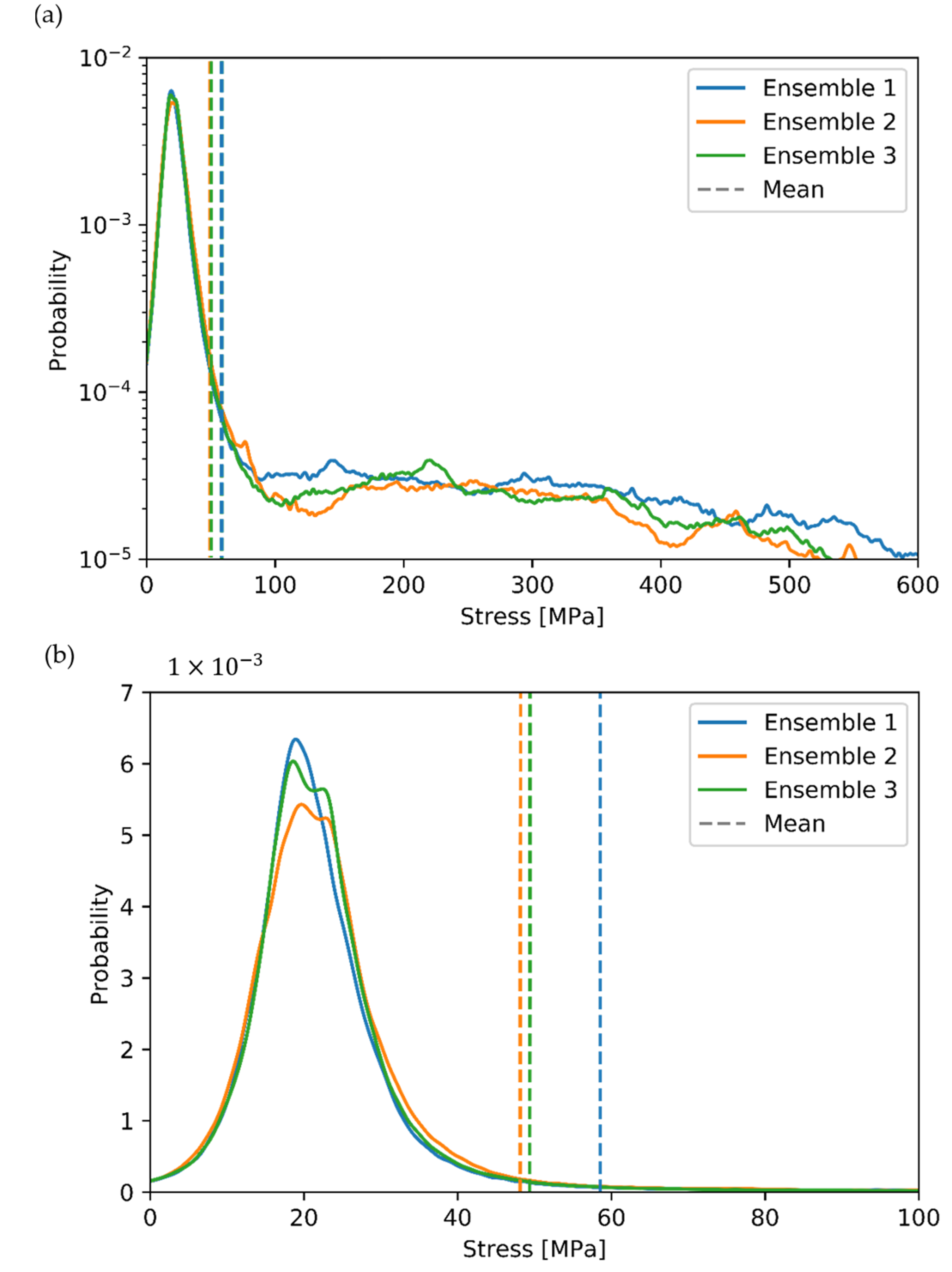
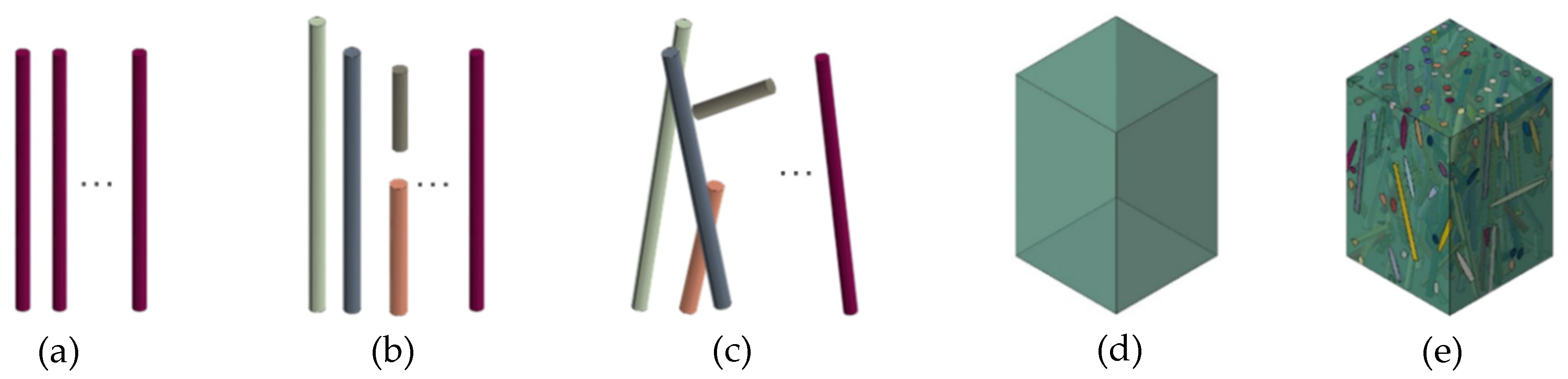
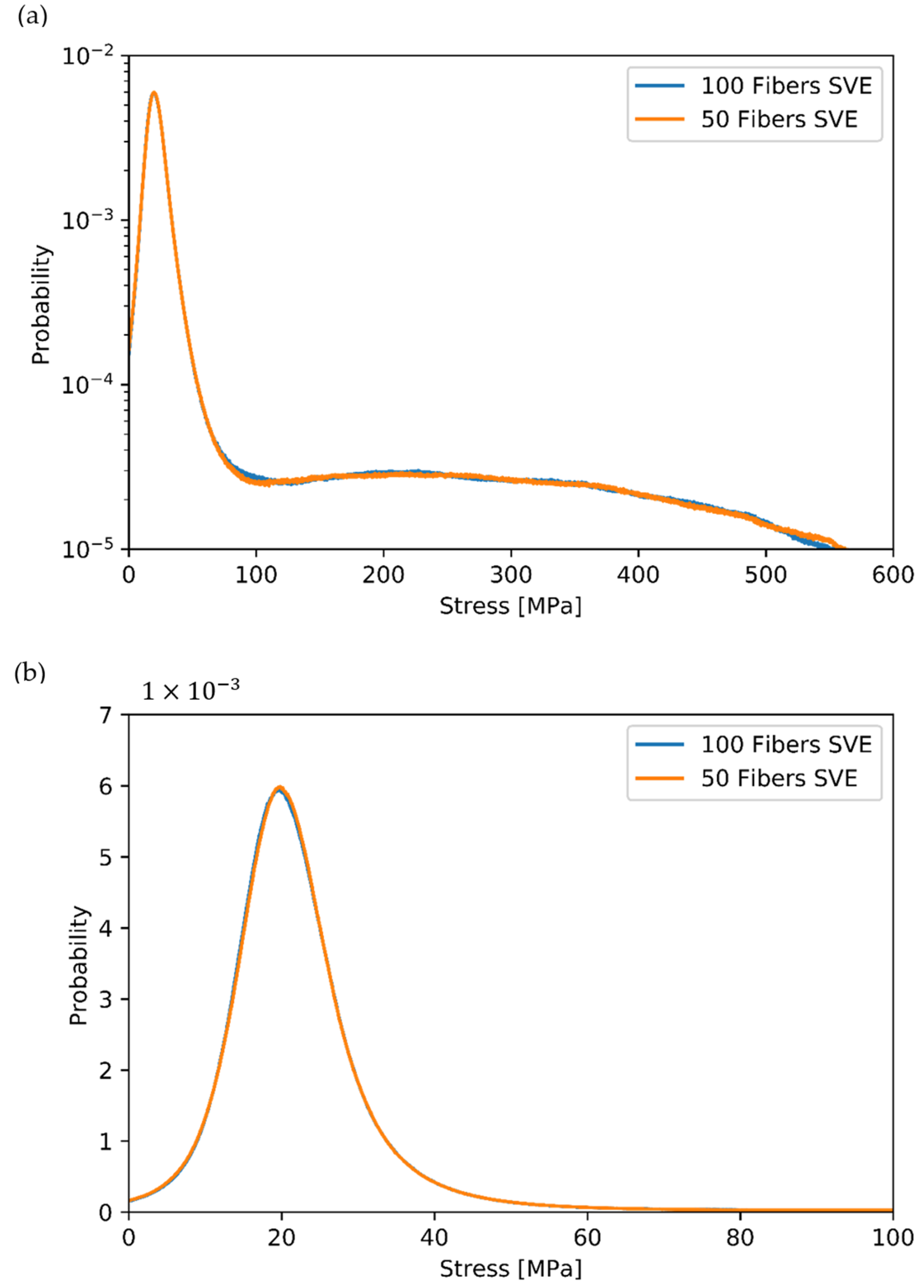
3.1. Influence of Finite Volume Approaches

The two approaches, SVE and RVE, respectively, are each investigated using 100 fibers in 60 different fiber ensembles. The evaluation is presented as histograms of the effective composite stiffness in Figure 8. A normal distribution is here assumed as null hypothesis, not rejected by the D’Agostino–Pearson test [35,36] with p-values of 0.365 (SVE) and 0.629 (RVE) being each greater than a selected significance level α = 0.05. In addition to the histograms Figure 8 shows the normal distributions and their mean values and the experimentally determined value of the mechanical characterization of the PBT-GF20.
The mean values of both approaches differ from each other with 5.269 MPa (SVE) and 5.300 MPa (RVE) only by 0.6%. The fact that both mean values deviate only slightly validates the assumption made in Section 2. The reason for this is that the average fiber volume fraction r = 1 n v f , r n of the SVE approach is equal to the given fiber volume fraction, which is realized in each RVE ensemble. However, more interesting at this point is the different standard deviation of the effective composite stiffness. The absolute value of the standard deviation is 235 MPa for the SVE approach and 151 MPa for the RVE approach, respectively. As the standard errors are sufficiently small at 30.0 MPa (SVE) and 19.5 MPa (RVE), the standard deviation is determined in sufficient accuracy by the 60 samples.

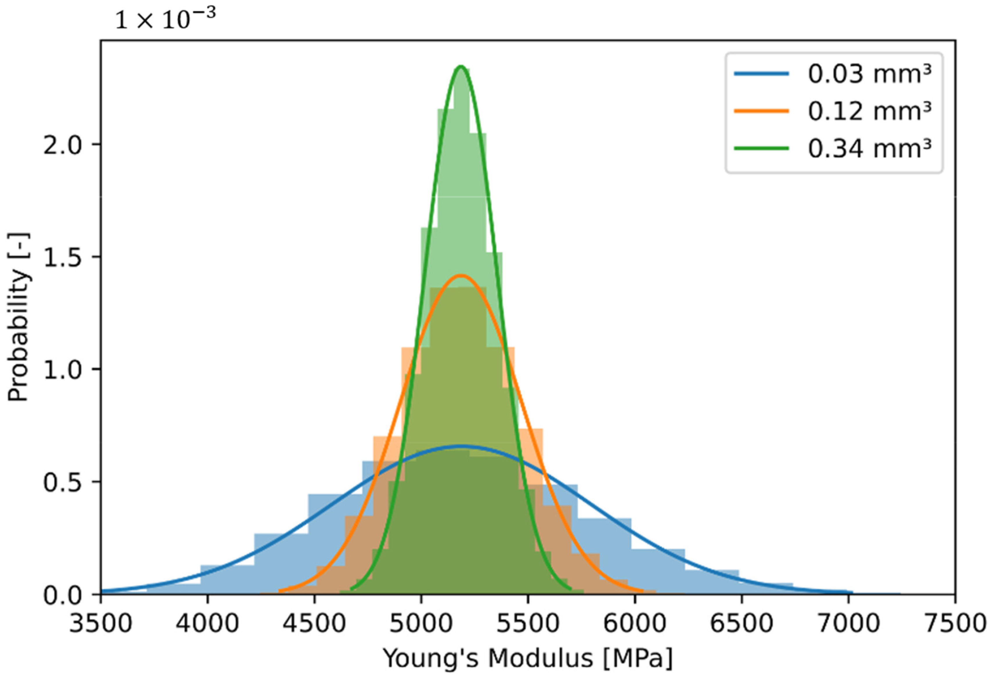
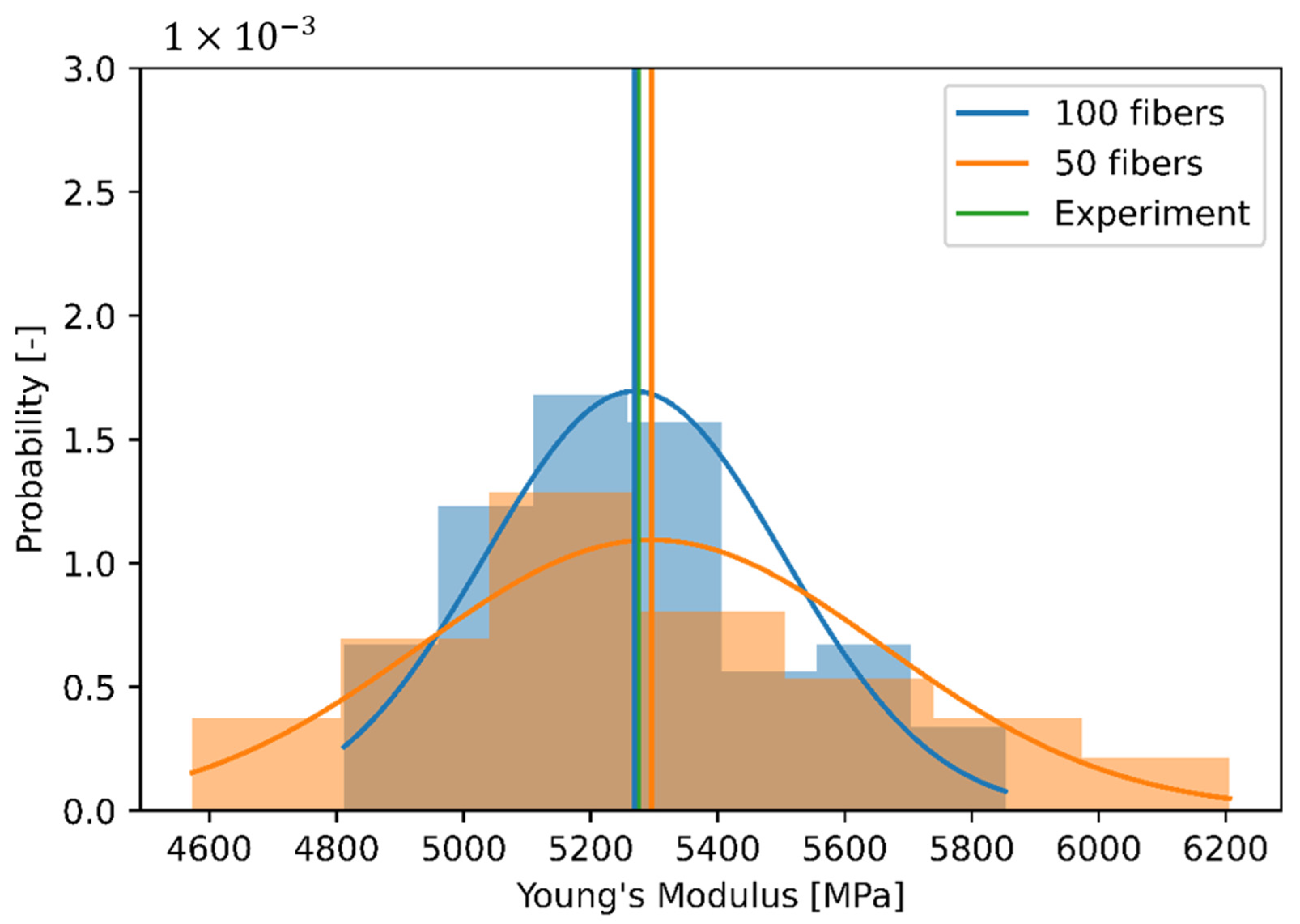
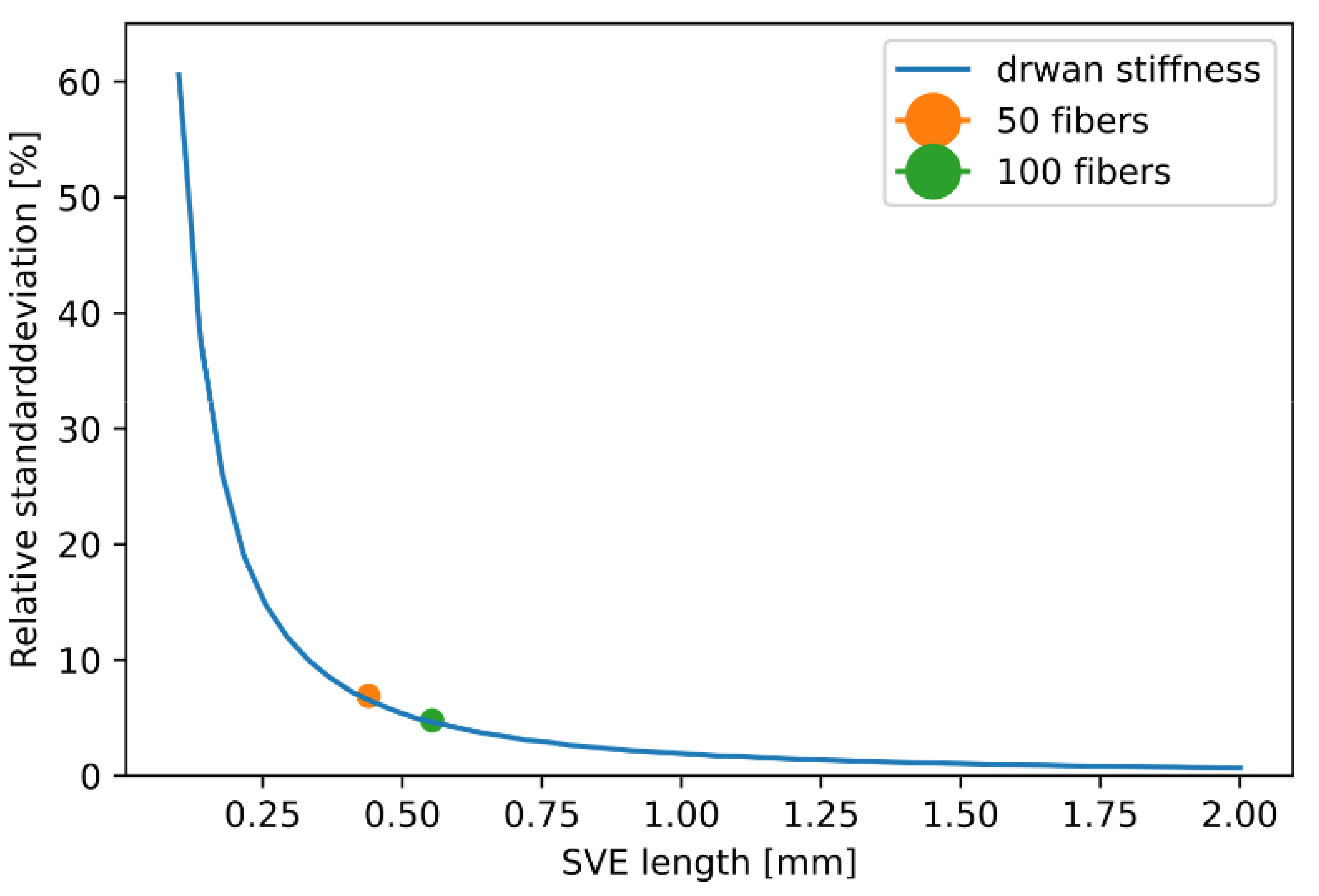
3.2. Influence of Finite Volume Size

Next, the influence of volume size on the standard deviation of the effective composite stiffness is investigated. The aim of this section is to prove that the standard deviation is a function of the volume under consideration. For this purpose, the SVE approach is used since the volume is constant in every realization. The investigation is carried out with 50 and 100 fibers, again with 60 fiber ensembles each. The number of fibers is of course proportional to the volume. Figure 9 shows the result of the Monte-Carlo simulation, analogous to Figure 8.
The p -values of the distributions are 0.365 (100 fibers) and 0.255 (50 fibers), not rejecting the null hypothesis of a normal distribution. The mean values are 5269 MPa with 100 considered fibers and 5296 MPa with 50 fibers. Thus, both mean values differ only very slightly with 0.5% from each other. However, the scattering is significantly more pronounced with 50 fibers than with 100 fibers. Correspondingly, the standard deviation is larger with 364 MPa to 235 MPa. The standard errors are 47 MPa (50 fibers) and 30 MPa (100 fibers), respectively, which shows that enough samples are considered.
The Monte-Carlo simulations with 50 and 100 fibers could be repeated in principal for any fiber numbers to work out the influence of the considered volume on the standard deviation. However, this is not very effective, as it would require a lot of computing costs, especially at a higher number of fibers. Therefore, the influence of the considered volume is worked out by a statistical analysis of the already available simulations results using 50 and 100 fibers. This procedure requires the stress probability within the fiber ensembles. Exemplarily, the stress probability of three randomly selected fiber ensembles, at a volume averaged strain of 0.01, is shown in Figure 10a. The probability plotted is defined as the normalized probability of stress at each node of the finite element model, weighted by the integration weight of the corresponding node. The volume averaged stress of the entire composite is also shown as a dashed line. The first peak of the probability plot is caused by the matrix phase, which is shown separately in Figure 10b. Note that the mean value shown in Figure 10b is also the mean value of the composite, not of the matrix phase.
An interesting side aspect for this study can also be derived from Figure 10b. A high volume-averaged mean stress of the composite (Ensemble 1) does not necessarily indicate a high matrix stressing. In fact, the probability of critical stresses above 35 MPa (cf. tensile tests in Section 3) is lowest for Ensemble 1 and highest for Ensemble 2, which has the lowest volume-averaged mean stress of the composite. If an initial local matrix failure is assumed as the main failure criterion for a composite, Ensemble 2 has the highest probability of failure. Consequently, a volume-averaged mean stress of the composite does not seem to be an appropriate failure criterion since the volume-averaged stress of the composite corresponds not necessarily to a high probability of high matrix stress above a critical value.
Figure 11 shows the average stress distribution of all 60 fiber ensembles for 50 and 100 fibers each. Figure 11a shows the entire composite and Figure 11b the matrix phase for a better differentiation. In both figures it is evident that the stress distributions are almost identical. This implies that this representation is independent of volume and can therefore be assumed as a statistical population. Additional samples do not further change the stress distribution. The assumption of the statistical population means that all possible stresses within the composite are covered and their statistical probability of occurrence is known. It should be noted that there must be a minimum number of fibers per ensemble so that a statistical population can be determined. This becomes evident from the scenario of an ensemble with a single fiber, which shows no variation in fiber arrangement and therefore no variation in the stressing of the fibers.
The assumption of the average stress distribution of all fiber ensemble as a statistical population allows a procedure to determine the volume-dependent distribution of the composite stiffness. The procedure is structured as follows:
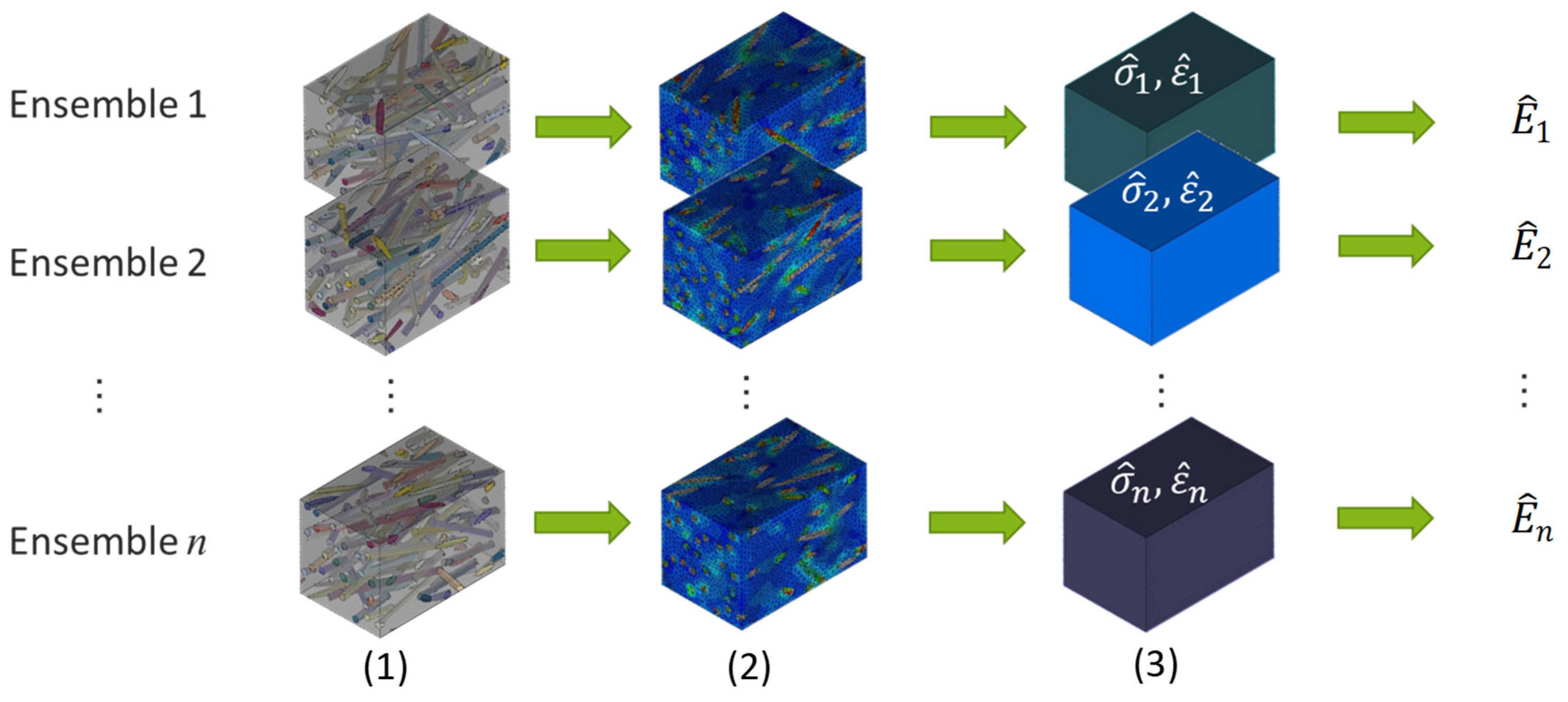
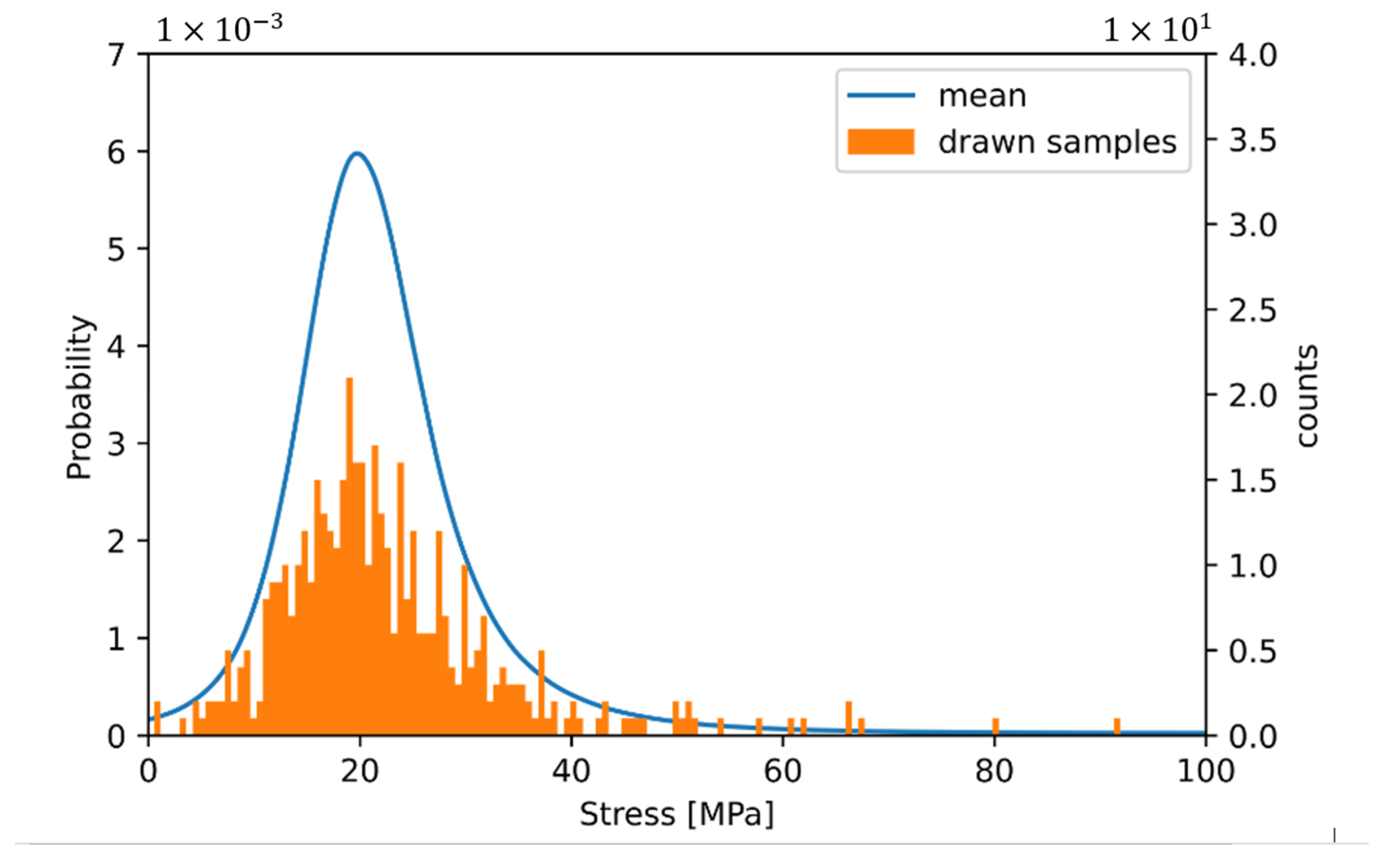
  • Sampling stress values from a statistical population;
  • Calculating mean value of samples;
  • Calculating stiffness out of mean of samples with global strain;
  • Repeating steps 1–3 several times to achieve stiffness distribution;
  • Repeating steps 1–4 for different volumes.
In step one, stress samples are generated from the statistical population according to their probability. Hereby, the number n d of values drawn is proportional to a volume V S being considered. The relationship is
V S = n d n S T ,
where n S T is the total number of discretization grid points of the statistical population. Here, it should be recalled that the stress probability is normalized. The physical unit of the volume V S is defined by the unit system used in FEA—in this investigation it is µm.
Figure 12 illustrates the sampling procedure using the matrix phase. It shows the statistical population for the matrix stress as well as 500 samples drawn from the population. The samples are shown as a histogram.
The sampling can be carried out separately for matrix and fiber phase, or directly combined for the composite. Thus, the sampling can be conducted within the SVE (combined) or RVE (separated) approach. In the case of the RVE approach, the exact ratio of the samples of the matrix and the fibers must be ensured so that the volume ratio corresponds to that used for the Monte-Carlo simulation. For further investigation in this paper, the samples are taken from the stress distribution of the composite, i.e., the SVE approach is used.
To calculate the effective composite stiffness from the drawn stress values, the arithmetic mean value of the drawn stress values is first calculated. Then, the stiffness is determined according to Equation (1) (here: 1% volume averaged strain).
A distribution of the stiffness can be generated by a repeated procedure, which is performed here as an example with three selected volumes. The selected volumes are calculated by V = l 3 with l = 300 µm, 500 µm and 700 µm. For these volume numbers, 10,000 repetitions of the drawing of stiffness values are made and the result is shown in Figure 13 as histogram and normal distribution. To avoid large numbers, the unit is converted to mm3 in the legend. The identical mean value of the three stiffness distributions and the different scattering are clearly visible. The largest scattering is the sampling with the smallest volume and vice versa.
The standard deviation determined from the drawn stiffness distributions can be further represented as a function of size and is shown in Figure 14. The representation over one edge length, with l = V 3 , is chosen for better understanding in the context of a component design. Furthermore, the standard deviation is shown relative to the mean value of the composite stiffness. The values are directly taken from the Monte-Carlo simulations of 50 and 100 fibers and are used as validation of the sampling method. The values of the Monte-Carlo simulation and the sampling procedure match very well. This validates the sampling procedure for determining the size-dependent standard deviation from a statistical population.
A main result of this study is the exact relationship between standard deviation and edge length: with increasing edge length, the relative standard deviation of the effective composite stiffness decreases rapidly and is negligible for large edge lengths. For smaller edge length, however, the deviation is not negligibly small. This seems particularly important against the background of a fiber orientation (Figure 5), which is only constant for a small length, especially in thickness direction of shell-like components.

4. Discussion

According to the current state of the art, mean values of effective composite stiffness are usually considered when designing components made of short fiber reinforced plastics [37]. This is based on the assumption that the volume of interest in a component design is very large and the scatter of the mean properties is therefore small. This assumption is to be discussable against the background of the results of the study shown (cf. Figure 14).
The influence of a local scattering of the composite stiffness on the component level will be shown. For this purpose, a tensile test specimen is numerically analyzed in the following with consideration of the local scattering of the composite stiffness. The composite is modelled as a liner–elastic material. A tensile specimen according to DIN EN ISO 527, type 1BA (Figure 4) is used for this purpose. For simplification, only the boundary layer with a homogeneous fiber orientation is considered in the analysis. With this simplification, the effect of scattering by the fiber ensembles can be separated from the effect of scattering by the fiber orientation.
The numerical analyzation is carried out with two selected mesh sizes, 1.0 mm edge length in the first case and 0.25 mm in the second case. The used elements are quadratic brick elements (C3D20). For each node of the finite element model the modulus of elasticity is drawn according to the values of a normal distribution calculated in Section 4 with respect to the selected mesh size. The mean value of this normal distribution in both cases is 5300 MPa and the standard deviations are 1060 MPa (0.25 mm) and 132.5 MPa (1.0 mm).
As a boundary condition for the FEA of the test specimen, one end of the specimen is fixed, and a displacement of 1 mm is applied to the opposite end. As a result, the von-Mises stress is shown in Figure 15.
The FEA with 1.0 mm mesh size yields a nearly constant stress of approximately 83 MPa with a maximum scattering of ±1.0 MPa. However, with the finer mesh an inhomogeneous stress distribution of the tensile test specimen due to the scattering of the composite stiffness is clearly visible. In an enlarged section of the surface, stress values between about 75 and 95 MPa occur. From the results two main points can be derived. First, the stresses on macroscopic scale can differ from those calculated by a purely mean-based model. A design based on constant value would therefore not be able to take the locally occurring higher stresses into account. This involves the potential risk that the design of the components is not sufficiently safe against mechanical failure. Second, the scattering of stress values is mesh-dependent, with a greater deviation at a finer mesh size. Obviously, it does not make sense to reduce the mesh size more and more until the limit of the assumption of the composite as a continuum is reached, or rather to model induvial fibers in component analysis. Instead, it seems to be more useful to develop a material model that can determine the scattering of stress on a statistical basis. Especially in a critical section of a component, this would provide import information for the design process of short fiber reinforced plastics.

5. Conclusions

In this research the statistical deviation of the effective stiffness of a short fiber reinforced composite is investigated. For this purpose, a Monte-Carlo simulation of finite volume models is performed. The finite volume model is defined by two different approaches. One is the RVE approach, where the fiber volume fraction is fixed for each realization of the finite volume. On the other hand, the SVE approach, where the fiber volume fraction may differ for each realization, is used. With both approaches the mean value of the effective composite stiffness calculated from the Monte-Carlo simulations is identical, but the scattering is different. With the SVE approach, the standard deviation is larger due to the fluctuating fiber volume content. Therefore, if the standard deviation is of interest, the SVE approach should be used. If only the mean properties are to be calculated, the RVE can be more efficient since fewer realizations are required to reach a certain confidence level.
Besides the influence of a locally varying fiber volume content, the influence of the finite volume size is considered. For this purpose, the volume-dependent standard deviation of the effective composite stiffness is calculated in this investigation using sampling of the statistical population. With this procedure it becomes evident that the smaller the volume, the greater the standard deviation. If the volume of interest is small enough, for example edge length < 0.25 mm, the standard deviation can become meaningful. In the context of dimensioning technical plastic parts this means that stresses and strains on a macroscopic level, caused by an applied external load, can be significantly affected by statistical fluctuations on the fiber scale. These fluctuations occur not only within one component, but also over different components. Modelling techniques based solely on mean values cannot take these fluctuations into account and can lead to inaccurate component design.

Author Contributions

Methodology, K.B., M.S., A.S.; software, K.B.; writing—original draft preparation, K.B.; writing—review and editing, M.S, A.S. supervision, M.S. All authors have read and agreed to the published version of the manuscript.

Funding

This research project was funded by the Deutsche Forschungsgemeinschaft (DFG, German Research Foundation) STO 910/13-1.

Institutional Review Board Statement

Not applicable.

Informed Consent Statement

Not applicable.

Data Availability Statement

The data is not publicly available.

Conflicts of Interest

The authors declare no conflict of interest. The funders had no role in the design of the study; in the collection, analyses, or interpretation of data; in the writing of the manuscript, or in the decision to publish the results.

References

  1. Duschlbauer, D.; Pettermann, H.E.; Böhm, H.J. Mori–Tanaka based evaluation of inclusion stresses in composites with nonaligned reinforcements. Scr. Mater. 2003, 48, 223–228. [Google Scholar] [CrossRef]
  2. Mori, T.; Tanaka, K. Average stress in matrix and average elastic energy of materials with misfitting inclusions. Acta Metall. 1973, 21, 571–574. [Google Scholar] [CrossRef]
  3. Benveniste, Y. A new approach to the application of Mori-Tanaka’s theory in composite materials. Mech. Mater. 1987, 6, 147–157. [Google Scholar] [CrossRef]
  4. Doghri, I.; Quar, A. Homogenization of two-phase elasto-plastic composite materials and structures: Study of tangent operators, cyclic plasticity and numerical algorithms. Int. J. Solids Struct. 2003, 40, 1681–1712. [Google Scholar] [CrossRef]
  5. Eshelby, J.D. The Determination of the Elastic Field of an Ellipsoidal Inclusion, and Related Problems. Proc. R. Soc. Lon. Ser. A 1957, 241, 376–396. [Google Scholar]
  6. Sun, C.T.; Vaidya, R.S. Prediction of composite properties from a representative volume element. Compos. Sci. Technol. 1996, 56, 171–179. [Google Scholar] [CrossRef]
  7. Sab, K. On the homogenization and the simulation of random materials. Eur. J. Mech. A Solids 1992, 11, 585–607. [Google Scholar]
  8. Akpoyomare, A.I.; Okereke, M.I.; Bingley, M.S. Virtual testing of composites: Imposing periodic boundary conditions on general finite element meshes. Compos. Struct. 2017, 160, 983–994. [Google Scholar] [CrossRef]
  9. Gusev, A.A. Representative volume element size for elastic composites: A numerical study. J. Mech. Phys. Solids 1997, 45, 1449–1459. [Google Scholar] [CrossRef]
  10. Okereke, M.I.; Akpoyomare, A.I. A virtual framework for prediction of full-field elastic response of unidirectional composites. Comput. Mater. Sci. 2013, 70, 82–99. [Google Scholar] [CrossRef]
  11. Schneider, M.; Ospald, F.; Kabel, M. Computational homogenization of elasticity on a staggered grid. Int. J. Numer. Methods Eng. 2016, 105, 693–720. [Google Scholar] [CrossRef]
  12. Hill, R. Elastic properties of reinforced solids: Some theoretical principles. J. Mech. Phys. Solids 1963, 11, 357–372. [Google Scholar] [CrossRef]
  13. Drugan, W.J.; Willis, J.R. A micromechanics-based nonlocal constitutive equation and estimates of representative volume element size for elastic composites. J. Mech. Phys. Solids 1996, 44, 497–524. [Google Scholar] [CrossRef]
  14. Gitman, I.M.; Askes, H.; Sluys, L.J. Representative volume: Existence and size determination. Eng. Fract. Mech. 2007, 74, 2518–2534. [Google Scholar] [CrossRef]
  15. Brisard, S.; Dormieux, L. FFT-based methods for the mechanics of composites: A general variational framework. Comput. Mater. Sci. 2010, 49, 663–671. [Google Scholar] [CrossRef] [Green Version]
  16. Wang, Z.; Smith, D.E. Numerical analysis on viscoelastic creep responses of aligned short fiber reinforced composites. Compos. Struct. 2019, 229, 111394. [Google Scholar] [CrossRef]
  17. Babu, K.P.; Mohite, P.M.; Upadhyay, C.S. Development of an RVE and its stiffness predictions based on mathematical homogenization theory for short fibre composites. Int. J. Solids Struct. 2018, 130–131, 80–104. [Google Scholar] [CrossRef]
  18. Berger, H.; Kari, S.; Gabbert, U.; Rodríguez-Ramos, R.; Bravo-Castillero, J.; Guinovart-Díaz, R. Evaluation of effective material properties of randomly distributed short cylindrical fiber composites using a numerical homogenization technique. J. Mech. Mater. Struct. 2007, 2, 1561–1570. [Google Scholar] [CrossRef] [Green Version]
  19. Chen, L.; Gu, B.; Tao, J.; Zhou, J. The average response and isotropy of 3D representative volume elements for random distributed short fibers reinforced elastomer. Compos. Struct. 2019, 216, 279–289. [Google Scholar] [CrossRef]
  20. Pan, Y.; Iorga, L.; Pelegri, A.A. Analysis of 3D random chopped fiber reinforced composites using FEM and random sequential adsorption. Comput. Mater. Sci. 2008, 43, 450–461. [Google Scholar] [CrossRef]
  21. Chen, L.; Gu, B.; Zhou, J.; Tao, J. Study of the Effectiveness of the RVEs for Random Short Fiber Reinforced Elastomer Composites. Fibers Polym. 2019, 20, 1467–1479. [Google Scholar] [CrossRef]
  22. Pan, Y.; Iorga, L.; Pelegri, A.A. Numerical generation of a random chopped fiber composite RVE and its elastic properties. Compos. Sci. Technol. 2008, 68, 2792–2798. [Google Scholar] [CrossRef]
  23. Burgarella, B.; Maurel-Pantel, A.; Lahellec, N.; Bouvard, J.-L.; Billon, N.; Moulinec, H.; Lebon, F. Effective viscoelastic behavior of short fibers composites using virtual DMA experiments. Mech. Time-Depend. Mater. 2019, 23, 337–360. [Google Scholar] [CrossRef]
  24. Wang, L.; Nygren, G.; Karkkainen, R.L.; Yang, Q. A multiscale approach for virtual testing of highly aligned short carbon fiber composites. Compos. Struct. 2019, 230, 111462. [Google Scholar] [CrossRef]
  25. Breuer, K.; Stommel, M. RVE modelling of short fiber reinforced thermoplastics with discrete fiber orientation and fiber length distribution. SN Appl. Sci. 2019, 2, 91. [Google Scholar] [CrossRef] [Green Version]
  26. Görthofer, J.; Schneider, M.; Ospald, F.; Hrymak, A.; Böhlke, T. Computational homogenization of sheet molding compound composites based on high fidelity representative volume elements. Comput. Mater. Sci. 2020, 174, 109456. [Google Scholar] [CrossRef]
  27. Greco, A. FEM analysis of the elastic behavior of composites and nanocomposites with arbitrarily oriented reinforcements. Compos. Struct. 2020, 241, 112095. [Google Scholar] [CrossRef]
  28. Huet, C. Application of variational concepts to size effects in elastic heterogeneous bodies. J. Mech. Phys. Solids 1990, 38, 813–841. [Google Scholar] [CrossRef]
  29. Hazanov, S.; Huet, C. Order relationships for boundary conditions effect in heterogeneous bodies smaller than the representative volume. J. Mech. Phys. Solids 1994, 42, 1995–2011. [Google Scholar] [CrossRef]
  30. Kanit, T.; Forest, S.; Galliet, I.; Mounoury, V.; Jeulin, D. Determination of the size of the representative volume element for random composites: Statistical and numerical approach. Int. J. Solids Struct. 2003, 40, 3647–3679. [Google Scholar] [CrossRef]
  31. Celanese. Celanex 2300 GV1/20 Datasheet. Available online: http://catalog.ides.com/Datasheet.aspx?I=26793&E=73487 (accessed on 28 April 2021).
  32. Kaiser, J.-M.; Stommel, M. Modified mean-field formulations for the improved simulation of short fiber reinforced thermoplastics. Compos. Sci. Technol. 2014, 99, 75–81. [Google Scholar] [CrossRef]
  33. Parra-Venegas, E.J.; Campos-Venegas, K.; Martinez-Sanchez, R.; Herrera-Ramirez, J.M.; Rodriguez-Miranda, A. The Tensile Behavior of E-glass fibers. Microsc. Microanal. 2012, 18, 784–785. [Google Scholar] [CrossRef]
  34. Breuer, K.; Stommel, M.; Korte, W. Analysis and Evaluation of Fiber Orientation Reconstruction Methods. J. Compos. Sci. 2019, 3, 67. [Google Scholar] [CrossRef] [Green Version]
  35. D’Agostino, R.B. An omnibus test of normality for moderate and large sample size. Biometrika 1971, 58, 341–348. [Google Scholar] [CrossRef]
  36. D’Agostino, R.B.; Pearson, E.S. Tests for departure from normality. Biometrika 1973, 60, 613–622. [Google Scholar]
  37. Gandhi, U.N.; Goris, S.; Osswald, T.A.; Song, Y.-Y. Discontinuous Fiber-Reinforced Composites, 1st ed.; Hanser: Munich, Germany, 2020. [Google Scholar]
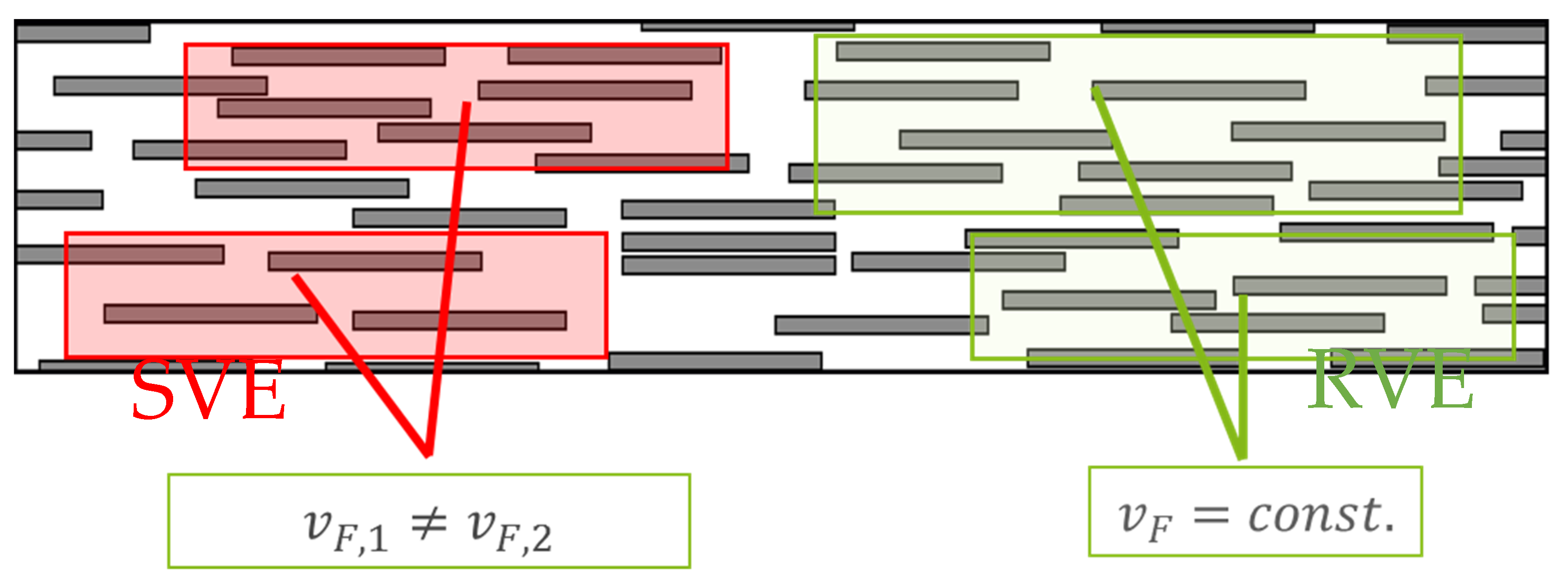
Figure 1. Procedure of the creation of a model with a unique fiber ensemble. (a): Considering the number of fibers. (b): Fiber length according to LDF. (c): Spatial orientation of fibers according to ODF. (d): Determining volume. (e): Placing fibers to achieve periodic microstructure.
Fibers 09 00032 g001
Figure 2. Two different approaches to define the finite volume: Statistical Volume Element (SVE) with constant dimensions and Representative Volume Element (RVE) with constant fiber volume fraction.
Fibers 09 00032 g002
Figure 3. Method of homogenization: creation of the microstructure (1), use of FEM to determine local stresses and strains (2), volume averaging (3) and calculation of effective modulus (4).
Fibers 09 00032 g003
Figure 4. Mechanical characterization of PBT-GF20 and PBT by tensile testing of specimens milled out of injection molded plates. The tensile direction with the PBT-GF20 corresponds to the flow direction of the injection molding process (2-direction).
Fibers 09 00032 g004
Figure 5. Measured components of fiber orientation tensor through thickness of the plates.
Fibers 09 00032 g005
Figure 6. Reconstructed ODF by the maximum entropy method of the shown fiber orientation tensor of second order. The color shows the probability that a fiber points in this direction.
Fibers 09 00032 g006
Figure 7. Normalized histogram of experimentally measured fiber lengths. Mean aspect ratio of fiber length distribution is 15.4.
Fibers 09 00032 g007
Figure 8. Histograms, normal distributions and mean values of the effective stiffnesses, calculated with the RVE and SVE approach as well as mean value of experimentally measured stiffness. We used 100 fibers in 60 different fiber ensembles for both approaches.
Fibers 09 00032 g008
Figure 9. Histogram and normal distribution of the effective stiffness, calculated with 50 and 100 fibers using the SVE approach.
Fibers 09 00032 g009
Figure 10. (a) Stress distribution of three unique fiber ensembles (top), (b) Stress distribution of the matrix phase of the same ensembles (bottom).
Fibers 09 00032 g010
Figure 11. (a) Average stress distribution of the composite with 50 and 100 fibers (top). (b) Average stress distribution in the matrix phase with 50 and 100 fibers (bottom).
Fibers 09 00032 g011
Figure 12. Average stress distribution and illustration of drawn samples.
Fibers 09 00032 g012
Figure 13. Histogram of drawn effective stiffness in dependency of considered volume.
Fibers 09 00032 g013
Figure 14. Relative standard deviation of drawn effective stiffness in dependency of considered volume and relative standard deviation of Monte-Carlo simulations with 50 and 100 fibers.
Fibers 09 00032 g014
Figure 15. FEA with two different mesh sizes (top: 1.0 mm, bottom: 0.25 mm) of a test specimen with uniform fiber orientation under consideration of the statistical deviation of the effective Young’s modulus due to the effect of different fiber ensembles.
Fibers 09 00032 g015
Table 1. Comparison of the definition of parameters with the SVE and RVE approach.
ParameterSVERVE
number of fibersconstantconstant
fiber geometryconstantconstant
fiber lengthdefined by LDFdefined by LDF
fiber volume fractiondefined by fibers and total volumeconstant
total volumeconstantdefined by fibers and fiber volume fraction
fiber orientationdefined by ODFdefined by ODF
fiber arrangementrandomrandom
phase propertiesconstantconstant
Table 2. Parameters of the isotropic, linear–elastic material model used for the individual phases and parameter of linear elastic fit of the PBT-GF20 composite for comparison.
PhaseYoung’s-Modulus [MPa]Poisson’s Ratio
composite5275-
matrix20000.42 [32]
fibers73,000 [32,33]0.22 [32]
Publisher’s Note: MDPI stays neutral with regard to jurisdictional claims in published maps and institutional affiliations.

