

Depolarization of Light in Optical Fibers: Effects of Diffraction and Spin-Orbit Interaction


Scientific and Technological Center of Unique Instrumentation of the Russian Academy of Sciences, 117342 Moscow, Russia
Fibers 2021, 9(6), 34; https://0-doi-org.brum.beds.ac.uk/10.3390/fib9060034
Submission received: 25 March 2021
/
Revised: 24 April 2021
/
Accepted: 28 May 2021
/
Published: 1 June 2021
Abstract
:Polarization is measured very often to study the interaction of light and matter, so the description of the polarization of light beams is of both practical and fundamental interest. This review discusses the polarization properties of structured light in multimode graded-index optical fibers, with an emphasis on the recent advances in the area of spin-orbit interactions. The basic physical principles and properties of twisted light propagating in a graded index fiber are described: rotation of the polarization plane, Laguerre–Gauss vector beams with polarization-orbital angular momentum entanglement, splitting of degenerate modes due to spin-orbit interaction, depolarization of light beams, Berry phase and 2D and 3D degrees of polarizations, etc. Special attention is paid to analytical methods for solving the Maxwell equations of a three-component field using perturbation analysis and quantum mechanical approaches. Vector and tensor polarization degrees for the description of strongly focused light beams and their geometrical interpretation are also discussed.

1. Introduction
The polarization of light must be taken into account in many tasks of fiber optics communication and devices for coupling light in and from optical fibers. The polarization state of light does not change during propagation in a homogeneous, isotropic, non-dispersed medium [1,2]. Significant changes in the state and degree of polarization occur during propagation in an inhomogeneous medium and through optical fibers.
Multimode optical fibers have attracted considerable interest in recent years for telecommunications, imaging, fiber lasers and amplifiers, ultrafast photonics, etc. They can operate over a wide range of wavelengths and have high coupling efficiency. Besides this, they degrade weakly under the influence of nonlinear effects. However, imperfections and external perturbations cause mode mixing and random polarization, leading to a strong change in the polarization state. Consequently, it is important to analyze the dynamics of the modes propagating in multimode fibers (MMFs).
Many works have been devoted to the study of depolarization of light in various media. In [3,4] the depolarization of light in randomly inhomogeneous media was considered. Two depolarization mechanisms were shown: geometric and diffraction, due to the Rytov rotation [5,6] of the polarization plane and diffraction, respectively. In single mode optical fibers, the change in the input polarization is usually due to nonlinearity and birefringence of the medium [7,8,9]. Depolarization also occurs in optical fibers without birefringence. The degree of linear polarization of radiation in multimode graded-index fibers decreases with distance [10]. In [11] it is shown that the degree of linear polarization in multimode graded-index fiber decreases with distance according to the quadratic law due to the Rytov rotation of the polarization vector, and the degree of circular polarization is preserved. However, in the experiments [12], the conservation of the degree of polarization in the optical fiber was not observed. In [13], the rotation of the plane of polarization of sagittal rays during propagation in a multimode fiber was experimentally observed. In [14], the rotation of the speckle pattern created by circularly polarized light at the fiber output was calculated, corresponding to the reversal of the sign of circular polarization. In [15], it was experimentally shown that the angle of rotation of the speckle pattern depends on the angle at which the circularly polarized light beam is coupled to the fiber. These effects can be considered as a manifestation of the optical Magnus effect [14,15] and the optical spin-Hall effect resulting from spin-orbit coupling.
In [16,17], the quantum-mechanical formalism of coherent states was used to study the evolution of polarization in a multimode isotropic graded-index medium. It is shown that depolarization of light in an isotropic graded-index medium occurs due to the effects of diffraction and spin-orbit interaction, and this mechanism manifests itself for radiation with linear and circular polarization. The rotation of the polarization vector during propagation in a two-dimensional medium is considered. It is shown that the rotation of the polarization plane depends on the axial displacement and the angle of tilt of the incident beam to the fiber axis. The change in the degree of polarization is closely related to change in the degree of coherence of the radiation. Changes in the degree of polarization of partially coherent beams propagating in optical fibers were considered in [18,19,20].
One of the goals of this review is to present a general picture of the polarization-dependent light transmission through optical fibers associated with the spin-orbit interaction. Recently, the effects of spin-orbit interaction in graded-index (GRIN) media have been of great interest [16,17,21,22,23,24]. In [25,26,27,28], the propagation of polarized twisted light beams in a cylindrical graded-index optical fiber is investigated by solving the three-component field Maxwell equations. An operator approach to calculating the average values describing propagation of light beams is developed. Spin-dependent effects on twisted light beams propagating in an optical fiber are demonstrated by solving the full three-component field Maxwell equations using perturbation analysis. Polarization and nonparaxial effects are considered in conjunction. Mode splitting in a cylindrical graded-index optical fiber is shown using the perturbation analysis to solve the full Maxwell equations [26].
A detailed description of quantum mechanical methods, such as the coherent states method and the density matrix formalism, for considering the propagation of light in graded-index waveguides, taking into account polarization effects, is given. An operator method for studying the evolution of polarization in a graded-index optical fiber is discussed.
In addition, we emphasize that 2D and 3D degrees of polarization should be used to describe the polarization effects associated with the spin-orbit interaction, depending on whether paraxial or nonparaxial light beams are considered.
2. 2D Polarization
Conventional laser sources emit paraxial light rays that propagate almost parallel to each other. This means that the polarization of the light beam is bounded by a plane perpendicular to the propagation direction, so for circularly polarized light, any resulting spin must be aligned longitudinally along the propagation direction. In conventional optics, the fields are transversal, so the polarization can be well described by a set of Stokes parameters defined from 2 × 2 coherence matrix [1]. In [2], a unified theory of coherence and polarization of random electromagnetic fields is proposed, which can be used to investigate changes in polarization during the propagation of light beams.
The Maxwell equations for the electric field in an inhomogeneous medium are reduced to:
or
where is the wavenumber and is the dielectric permittivity of the medium.
In the paraxial approximation the Maxwell equations can be reduced to the equivalent time-independent Schrodinger equation [29]. In [16,17], a similar approach is used to obtain a parabolic equation for a two-component vector field. Since the paraxial beam propagates in a direction close to the z-axis, the conditions are valid. We have the following equation for the two-component wave function of the field, neglecting the term in Equation (2) [16,17]:
where ,
is the unperturbed Hamiltonian corresponding to the first two terms in Equation (2) and
is the Hamiltonian corresponding to the third term in the Equation (2).
The Hamiltonian can be rewritten in terms of annihilation and creation operators using the relations
Thus, we have
Here
, is the unit matrix and are the Pauli matrices.
The Pauli matrices satisfy the following relations:
The solution to Equation (7) can be expressed as
where is the evolution operator.
The polarization properties of the light are determined by the elements of the coherency matrix [1,2]:
where the angle brackets denote the average values over the statistical ensemble representing the fluctuating field. The degree of polarization is defined by the expression [1,2]
The evolution of the coherency matrix is determined by the expression [16,17]:
or the equation
where is the coherency matrix operator in the initial plane z = 0.
2.1. Rotation of Polarization Plane in a Graded Index Fiber
The polarization plane rotates on propagation of light on the helical trajectory [5,6]. In a single mode optical fiber wound on a cylinder, such rotation was observed experimentally [30] and interpreted in terms of Berry’s geometrical phase [31]. The rotation of the polarization plane was observed also in a straight multimode fiber with a step-index type profile [13]. It is also interesting to consider the reverse effect, i.e., the effect of polarization on the trajectory and width of the beam. When a light beam is reflected from an interface, the longitudinal shift of the gravity center of the beam is different for s- and p-polarized beams [32], while the transverse shift has reverse signs in the case of a right- and left-hand circularly polarized light beam [33]. In [34], lateral and angular shifts were shown for strongly focused azimuthally and radially polarized beams at the interface of dielectrics. In [14], the rotation of the speckle pattern created by circularly polarized light at the fiber output was shown, corresponding to the reversal of the sign of circular polarization. The dependence of the angle of rotation of the speckle pattern on the angle at which a circularly polarized light beam falls on the fiber input was experimentally demonstrated in [15].
It was shown in [35] that when light propagates along a helical trajectory in a graded-index fiber, a spin-dependent relative shift occurs between right-hand and left-hand circularly polarized light beams. This effect was observed for a laser beam propagating in a glass cylinder along a smooth helical trajectory [36]. Note that this shift is a manifestation of the optical Magnus effect [37] and the optical spin-Hall effect [38,39], which occurs due to the spin-orbit interaction. Beam and wave optics are used to analyze the propagation of light in graded-index media [40]. The effect of polarization on modes in lens-like media was analyzed in [41]. In [42], the polarization-dependent GH beam shift at the graded-index interface of dielectrics is studied. In [43], the beam shifts with respect to geometric optics caused by spin-orbit interaction and nonparaxiality in a graded-index optical fiber are investigated.
The methods of coherent states can be used to study the evolution of the parameters of a light beam. The operator approach is used to calculate the average values describing the light beam. These methods were used in [16,17] for investigation into the depolarization of light in a graded-index waveguide. A two-dimensional graded-index waveguide was considered:
where is the gradient parameter, is the refractive index along the axis of the waveguide, and x and y are the transverse coordinates of the waveguide.
In the input plane z = 0, we introduce coherent states represented by Gaussian wave packets:
where and define the initial coordinates of the center of gravity of the light beam and the tilt angles of the beam with respect to the axis of the medium.
Coherent states were first introduced by Glauber [44] in 1963 from the consideration of the states of the electromagnetic field oscillators and the study of its statistical properties. In essence, these states are analogous to the Gaussian wave packets, which were constructed and studied by Schrodinger [45] for the quantum harmonic oscillator as part of his study of the connection between the quantum and classical descriptions.
In [46,47], the coherent states method, the integral of motion and the density matrix formalism are used to describe the propagation of a paraxial optical beam and partially coherent radiation in a weakly inhomogeneous medium. The coherent states method is also valuable for considering the diffraction of partially coherent light beams by microlens arrays [48].
Coherent states (10) have the minimal width and diffraction-limited angular divergence on the propagation in a square-law-index medium. The center of such a wave packet propagates along the trajectory of the geometric ray corresponding to the ray optics. Besides, the coherent states (10) are generating functions for the waveguide modes and they form a complete set of functions. This property can be used to decompose an arbitrary beam field into a series of coherent states:
The trajectory and width of the beam are defined in terms of the matrix elements:
The wave functions of the light field linearly polarized along the x- and y-axes can be expressed as
The wave functions of right- and left-hand circularly polarized light have the form
or
The evolution of the operator is determined by the equation
where is the Hamiltonian of the system.
For a light beam linearly polarized along the x-axis with initial parameters x0 ≠ 0, y0 = 0, px0 = 0, and py0 = 0, we obtain the following expressions for the beam trajectory and beam width [35]:
For a light beam polarized along the y-axis, we have
It follows from Expressions (16) and (17) that the polarization of the radiation does not affect the path of the beam. However, the polarization effects affect the beam width, which fluctuates with a period equal to the beam oscillation period.
Additional fluctuations in the beam width in the direction of field polarization are shown in Equations (16) and (17). This effect is a first-order correction to the paraxial approximation. In [49,50] the dynamics of beam self-imaging by means of femtosecond laser pulse propagation in nonlinear GRIN multimode optical fibers was studied experimentally. It was shown that the periodical beam self-imaging acts symmetrically on both the x and y axis. The amplitude of the oscillations for the parameters of the graded-index fiber used in [49,50] is only 0.3% of the initial beam width, so it is likely that the effect was not observed in experiments.
For a circularly polarized light beam, the expressions for the trajectory and beam width with the initial parameters x0 ≠ 0, y0 = 0, px0 = 0, and py0 ≠ 0 have the form [35]:
where σ = +1 corresponds to right-hand circularly polarized radiation and σ = −1 corresponds to the left-hand circularly polarized light beam.
For circularly polarized light, the plane of propagation of the meridional beam (py0 = 0) rotates in the direction of circulation of the polarization vector. A similar rotation takes place for the sagittal rays (py0 ≠ 0). The rotation of the meridional ray and the additional rotation of the sagittal rays increase linearly with distance:
The following is a comparison between the Rytov rotation angle or the Berry phase of the polarization plane due to the twisting of the propagation path [17]:
the rotation angle of the plane of the meridional ray (19) is due to the circular nature of the polarization of light.
It follows from (19) and (20) that the values of these angles are equal to each other for , i.e., in the case when the axial shift of the incident beam is equal to the width of the fundamental waveguide mode .
In Figure 1, the angular shift dependence on the beam’s angular aperture (diffraction angular divergence) for the distance corresponding to the period of the beam twisting is presented. The angular GH shift increases in proportion to the square of the angular aperture of the beam. A similar effect was experimentally observed for a wave beam when a Gaussian beam falls on the air–glass interface [51]. Substantial positive and negative Goos-Hänchen shifts near the surface plasmon resonance were also shown in subwavelength gratings [52].
The polarization affects the width of the beam propagating in the waveguide. Below, we consider the paraxial propagation of a beam whose initial width is not matched with the fundamental mode of the waveguide. The analysis of the propagation of a strongly focused light beam in a graded-index waveguide is presented in [53,54].
For a linearly polarized axis beam (α = 0) with a field radius a0, the evolution of the beam width is defined by the expressions [43]:
where , , and is the gradient parameter, w0 is the radius of the fundamental mode.
At z = n0π/(2ω), the beam width takes the minimum value:
The minimum beam width of a circularly polarized beam is given by
It follows that the values of the minimum beam width decrease if the width of the incident beam is greater than the radius of the fundamental mode of the waveguide ().
Thus, the polarization effects cause an increase in the size of the focal spot. For linearly polarized light, the beam shows a broadening only in the direction of the plane of polarization, and the initially symmetric beam becomes elliptical. Such a broadening of the beam in the direction of the polarization plane was observed in experiments devoted to measuring the size of latex spheres [55].
The effect of polarization effects on the beam parameters is negligible in the case when the ratio of the gradient parameter to the wave number is small. However, when the beam is focused to a region smaller than the radiation wavelength, these effects become significant. This should be taken into account when analyzing experimental data, in particular the results of measurements using near-field microscopes.
Circular polarization leads to rotation of the plane of propagation of the meridional beam, as well as to additional rotation of the sagittal rays, and this rotation depends on the axial displacement of the incident beam. Both circular and linear polarizations lead to fluctuations in the beam width during propagation in a graded-index waveguide. Polarization affects the focus of the light beam in a graded index medium and is a limiting factor. In the case of linear polarization, the cross-section of the light beam in the plane of focus becomes elliptical, elongated in the direction of the plane of polarization.
2.2. Depolarization of Light
Depolarization of light propagating in a graded-index fiber was considered in [16,17]. It is shown that the spin-orbit interaction causes an asymmetry effect for the depolarization of right-hand and left-hand circularly polarized light. Depolarization is stronger if the helicity of the trajectory and the photons have the same signs, and weaker if they are not the same.
2.2.1. Linear Polarization
The fields of the linearly polarized beams are given in Equation (13). The coherency matrix is determined by the following matrix elements:
The coherence matrix operator in the plane z = 0 is defined by the source. For radiation linearly polarized along the x-axis, we have [1]
where I0 is the total intensity of the incident beam.
To solve Equation (8) and calculate the matrix elements (24), the commutation relations (i, j = 1, 2), the relationships (5) and the relations
can be used.
Solving Equation (8) up to a parameter η2 and substituting the solutions in Equation (7), we obtain the following expression for the value, determining the depolarization [16,17]:
Equation (28) includes a contribution of both sagittal and meridional rays with initial coordinates in the plane z = 0: x0 ≠ 0, y0 = 0, px0 = 0, py0 ≠ 0.
It follows that the depolarization depends on the wavenumber and disappears at λ → 0. For an axial beam (x0 = 0, py0 = 0), we obtain oscillations in the degree of polarization that are purely diffractive in origin. The effect of periodic retrieval of the initial degree of polarization should be observed in a single-mode isotropic optical fiber, when the fundamental mode of the optical waveguide is considered.
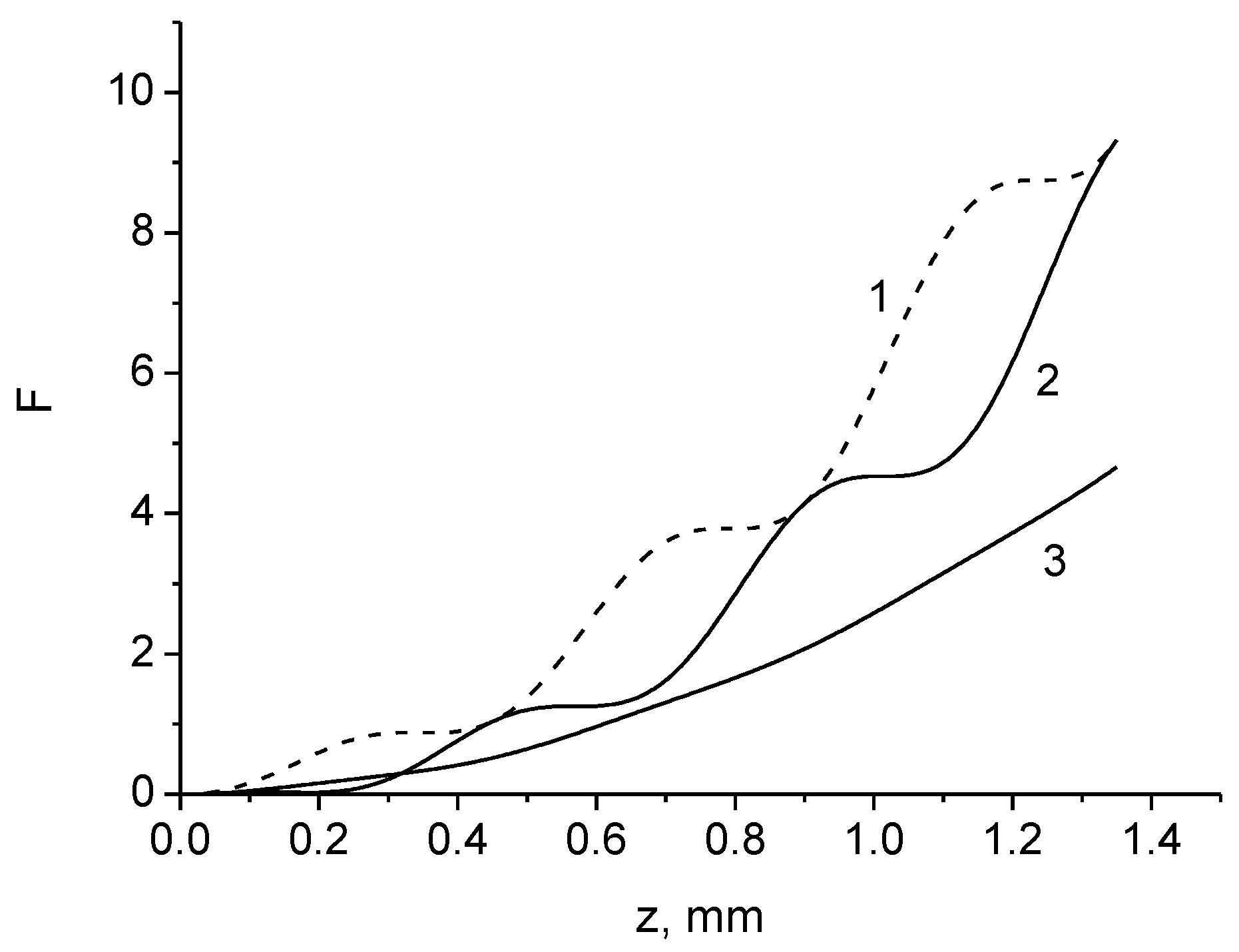
The dependence of the degree of polarization of linearly polarized light on the distance z is represented by the curves in Figure 2 for various offsets x0, including the meridional rays and the radius-preserving () spirally twisted sagittal rays. It is clear that the degree of polarization decreases inversely with the square of the distance. The decrease in the degree of polarization becomes more pronounced as the displacement or inclination of the beam relative to the fiber axis increases. The depolarization length of the meridional rays is 1.4 times longer than the depolarization length of the sagittal rays.
In Figure 3 the values as a function of the distance z are presented for meridional and sagittal rays. It can be seen that the increase in this value is accompanied by small fluctuations. The degree of polarization decreases quadratically with the increasing distance. Depolarization increases with an increase in the displacement of the axis or the inclination of the beam to the axis of the waveguide. The decrease in the degree of polarization is accompanied by small fluctuations. Note that Equation (28) is valid only for distances z ≤ z0, where the distance z0 is determined by the accuracy of the solution of Equation (8). In our case, this distance is equal to
The degree of polarization can be obtained by substituting Equation (28) into Equation (7):
The degree of polarization decreases with increasing distance, and depolarization disappears at λ → 0. There are fluctuations in the degree of polarization of purely diffractive origin in the case of the axial beam (x0 = 0, py0 = 0):
It follows that the degree of polarization of the axial beam takes its initial value at ωz = mπ (m = 1, 2, 3 …). The depolarization characteristics of the imaging probe with the multi-mode fiber with a length of 6.2 mm were studied in [56]. It is shown that the depolarization coefficient for the modal fields LP01 and LP21 can be estimated at 0.7.
2.2.2. Circular Polarization
The fields for right-handed and left-handed circularly polarized light are defined in Equation (14). The coherency matrix in the initial plane has the form [1]
The Jones vector describing linearly polarized light can be defined in terms of the Jones vector of circularly polarized radiation:
where is the transformation matrix.
The following expression describing the depolarization can be obtained by solving Equation (8) up to a small parameter η2 [16,17]:
The signs ± correspond to right-handed and left-handed circularly polarized light. The effect of asymmetry occurs with respect to the sign of twisting of the trajectory of sagittal rays (Figure 4). Depolarization is stronger if the helicity of the trajectory of rays and “photons” has the same signs, and less if they do not coincide. The depolarization of the meridional rays is less than that of the sagittal rays.
The following relations
are used to calculate the coherency matrix elements.
Substituting Equation (33) into (7), we obtain an expression for the degree of polarization
The degree of polarization at the distances z >> ω−1 may be defined as
The sagittal rays with constant radius of twisting (py0 = x0ω) are considered here. The degree of polarization decreases with increasing distance, similar to the degree of polarization of a linearly polarized beam. A similar result occurs in the case of left-handed polarized light.
2.3. Berry Phase and Degree of Polarization
The plane of polarization of a light beam rotates when it propagates along a curved trajectory in an inhomogeneous medium [5,6]. This rotation was experimentally demonstrated [30] in a single-mode fiber wound along a cylinder and interpreted as a geometric Berry phase effect [31]. The effect of a spin-dependent relative shift between right-and left-handed circularly polarized light beams propagating in a glass cylinder along a smooth helical trajectory was also observed [36]. A similar beam shift was shown in a graded index optical fiber [43]. This shift can be considered as a manifestation of the optical Magnus effect [14] and the optical spin-Hall effect [38,39], which occurs due to the spin-orbit interaction.
In [57], the evolution of the polarization plane and the Berry phase in a graded index waveguide was investigated using the quantum mechanical formation of coherent states.
The rotation angle of the polarization vector of a beam linearly polarized along the x-axis propagating along a helical trajectory is determined by the expression [57]:
The Expression (38) is valid for sagittal rays with initial coordinates .
For small values of the axial displacement of the beam, the Expression (38) has the form [57]:
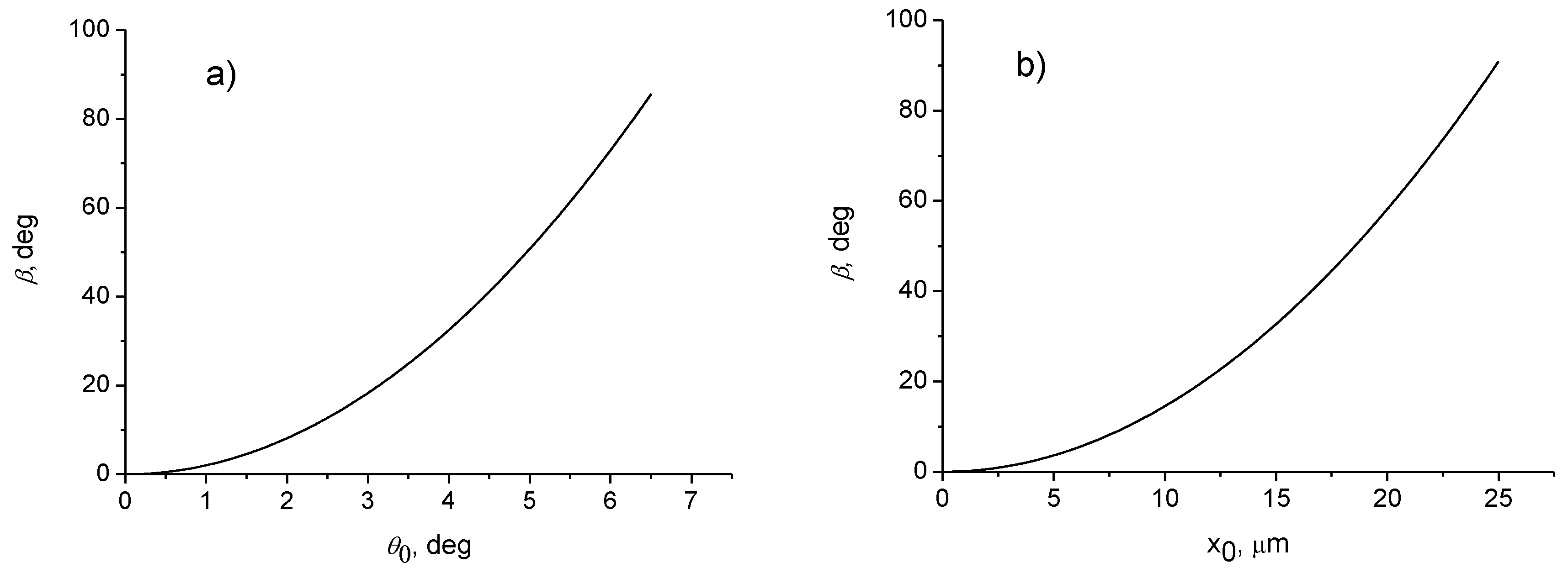
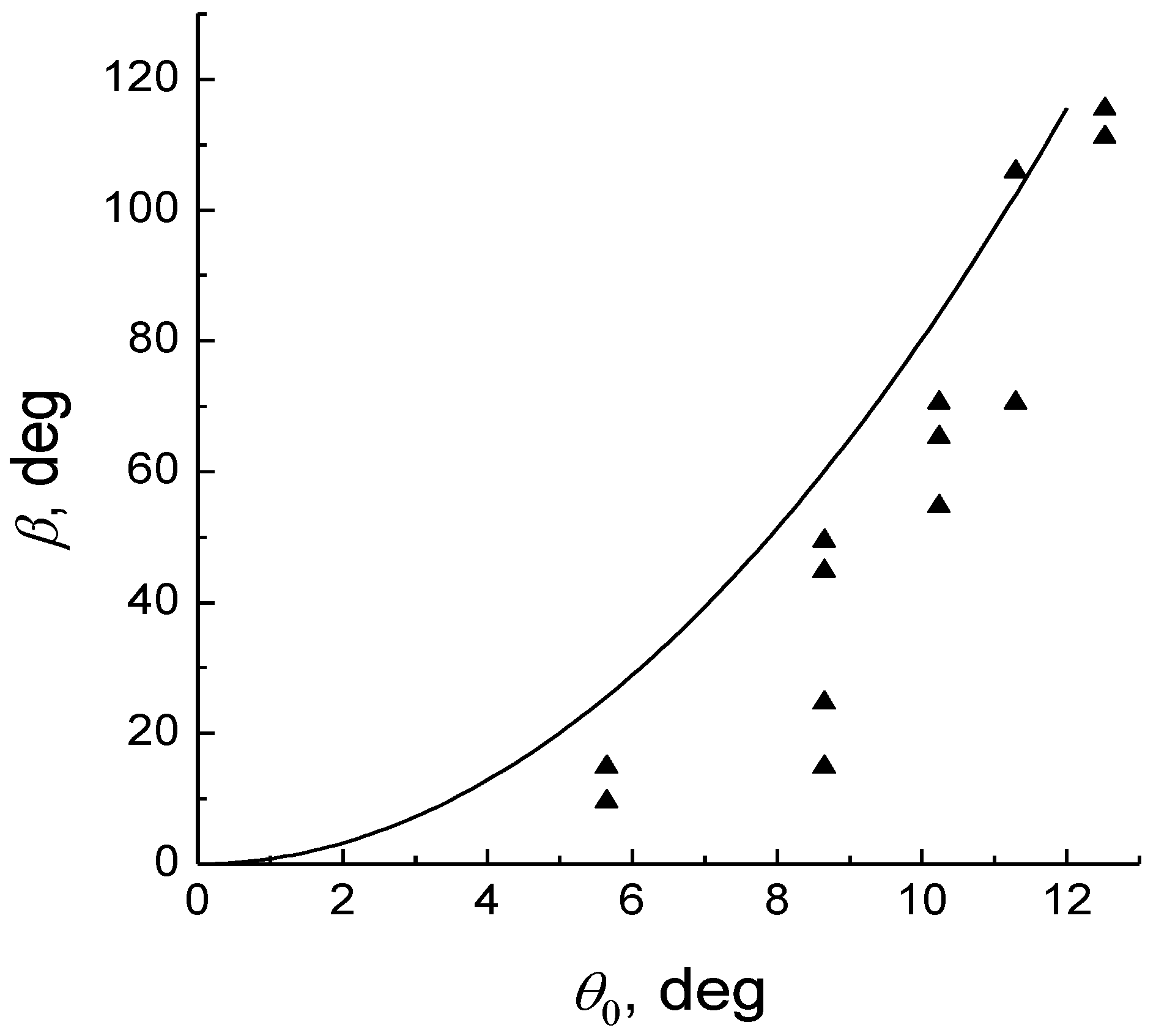
It can be seen from (39) that the rotation angle of the polarization plane increases quadratically with the angle of tilt θ (py0 = n0sinθ) of the beam to the waveguide axis or with the axis displacement x0 for sagittal rays with constant radius of twisting () (Figure 5a,b). The calculated results for the angle of rotation of the polarization plane are in good agreement with the experimental data [13]. Note that the cubic dependence of the rotation angle of the polarization vector on the angle between the propagation direction and the axis of the fiber with a step profile of the refractive index was obtained in [37].
The rotation speed of the polarization vector is defined by the expression
It follows that the rotation of the polarization vector is of irregular character. The rotation speed is zero at the points where the polarization vector is parallel to the main normal. Note that the Rytov’s rotation [5] or the Berry’s phase [31] have a geometrical origin and do not depend on the wavelength of the radiation. However, the variance of the Berry’s phase is of wave nature and disappears at λ → 0. Thus the variance of the Berry’s phase is equal to [57]
It can be seen that the dispersion of the Berry’s phase increases nonlinearly at small values of the axis displacement. The Berry’s phase dispersion for μm of the order of <δβ> ≈ 1° occurs at a distance of z ≈ 3.7 mm. This corresponds to the rotation of the polarization plane by an angle of <β> ≈ 4.4°.
It follows that the dispersion of the Berry’s phase is determined by the degree of polarization P. As noted in [29], the depolarization in an optical fiber with a length of z ≈ 7.5 cm is 10–30%, which is consistent with the results obtained (Figure 6). It can be seen that fluctuations in the Berry’s phase dispersion for the axial beam exist, although the phase is zero. In addition, the Berry’s phase fluctuations for the meridional rays increase with distance, although the Berry’s phase value is zero. Thus, measurements of the degree of polarization will verify experimentally the wave nature of the Berry’s phase.
The dispersion of the rotation angle of the polarization plane increases with distance and can be determined by measuring the degree of polarization of light. The dispersion of the Berry’s phase or the angle of rotation of the polarization plane increases with distance, and there are fluctuations in the Berry’s phase dispersion for the axial beam (fundamental mode), which have a wave nature.
3. 3D Polarization
In conventional optics, the fields are transverse, so the polarization can be well described by a set of Stokes parameters determined from the 2 × 2 coherence matrix [1,2]. However, the electromagnetic field in the far zone is transverse and for waves propagating along the z axis, Ez = 0, many problems of near-field optics, optical microscopy, data storage, and scattering need to be analyzed, taking into account the longitudinal component of the field Ez. Strongly focused beams contain a non-zero longitudinal component of the field , so we should consider 3 × 3 coherence matrices to describe them. The Stokes 2 × 2 formalism was extended to 3 × 3 coherence matrices, and the degree of polarization for arbitrary electromagnetic fields was introduced in [58,59,60,61]. The evolution of three-dimensional electromagnetic fields in a graded index medium is studied in [25,26,27,28,62]. The coherence matrix is represented in terms of spherical or rectangular tensors, similar to the Gell-Mann matrices. The evolution of the coherence matrix is defined in terms of the Hamiltonian obtained from the three-component Maxwell field equations.
The polarization state of the most general two-dimensional field can be completely described by three parameters. This is referred to as vector polarization. For a three-dimensional field, except for three components of the vector polarization, there are five components of tensor polarization. The complexity of the 3D electromagnetic field arises from the tensor polarization [59,60]. In contrast to the 2D case, where any beam of light can be represented as the superposition of totally polarized and unpolarized light, in the 3D case, an arbitrary beam cannot be represented as a mixture of an unpolarized beam (one parameter) and a polarized beam (five parameters) because nine independent parameters are needed to characterize the coherence matrix.
Maxwell’s equations for the electric field in a general inhomogeneous medium with dielectric constant are reduced to:
where is the wavenumber and is the dielectric constant of the medium, is the propagation constant.
Formally, taking the square root of both sides, we obtain an equation equivalent to the stationary Schrodinger equation for the reduced field :
where and are the eigenvalue and eigenfunction of the Hamiltonian, accordingly,
is the nonparaxial correction to the operator of paraxial propagation, which has the form
The Hamiltonian can be rewritten in terms of annihilation and creation operators in cylindrical coordinates [17,27,62]. This allows the averaged values describing the light beams to be calculated analytically.
3.1. Vector Laguerre–Gauss (LG) Beams in a Graded-Index Fiber
Diffraction and refraction forces govern a light beam propagating in an inhomogeneous medium in the scalar approximation. However, the vector Maxwell equations are the basis of a consistent electromagnetic theory of light propagation. To analyze the vector wave fields, the influence of additional effective forces associated with polarization (spin angular momentum (SAM)) and orbital angular momentum (OAM) should be taken into account. It is known that when the linearly polarized optical beam propagates along a spiral trajectory, the polarization vector undergoes a Rytov rotation [5,6].
In [28], the full three-component field Maxwell equations are solved to investigate the effect of polarization (spin) and OAM on the shape of a vortex light beam with a nonzero radial number propagating through a cylindrical graded-index fiber. Remote focusing and highly efficient transfer of a strongly focused spot in a graded-index waveguide are demonstrated in [54]. It is known that different paraxial modes or rays are periodically in phase as they propagate in graded-index optical waveguides, and periodic focusing can be observed [63]. However, nonparaxial effects destroy this periodic focusing. Surprisingly, the restoration of the initial beam shape and strong focusing occur at extremely large distances due to the revival effect caused by interference between propagating modes [28,54]. Expressions of the path and beam width describing nonparaxial propagation in graded-index (GRIN) media were obtained earlier in [64]. However, the resulting expressions do not include the revival effect. In [65,66], the correct expressions for the beam trajectories and widths are obtained, which contain the long-term period oscillations of the beam trajectory and its width. In [67], the revival effect in GRIN media was considered up to a second-order approximation. In [53,54,68,69,70], exact analytical expressions for the trajectory and width of nonparaxial wave beams are obtained. It should be noted that the revival effect in a cylindrical GRIN rod, which occurs during nonparaxial propagation, was also recently studied in [71]. However, the problem was considered in the framework of the scalar Helmholtz equation, which is not the case of nonparaxial propagation of a light beam in a cylindrical waveguide. In addition, Hermite–Gauss beams were considered as modal solutions, whereas for a cylindrical GRIN waveguide they may not be modal solutions.
Analytical solutions can be obtained for a rotationally symmetric graded-index optical fiber:
where is the refractive index on the waveguide axis, ω is the gradient parameter, , a is the waveguide radius.
The unperturbed Equation (44) has the form
where the Hamiltonian is given in (45).
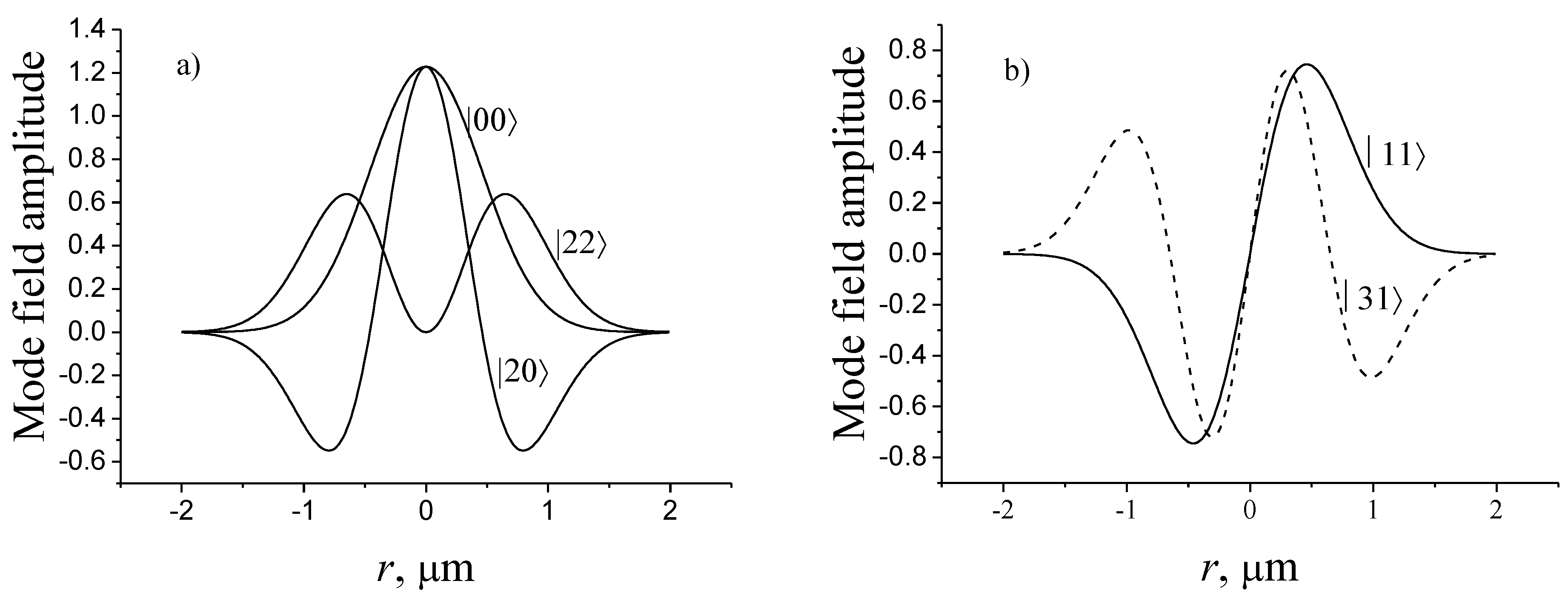
The solution of the unperturbed equation is described by the radially symmetric Laguerre–Gauss functions (LG) (Figure 7) [62]:
where is the principal quantum number, p and are the radial and azimuthal indices, accordingly, and or 0, , is the radius of the fundamental mode. The numbers and express the eigenvalues of the unperturbed Hamiltonian , and eigenvalues of the angular momentum operator .
The hybrid wave functions consisting of transverse and longitudinal components are solutions of Equation (43):
where and correspond to right-handed and left-handed circularly polarized beams, accordingly, and corresponds to the linear polarization.
There is no mode conversion at propagation if the incident beam is expressed by (48). Note that the hybrid wave function (48) cannot be factorized into the product of spin and orbital parts since the mixing of OAM and SAM exists. Thus, the modal solutions of the Maxwell equations in a GRIN media are the hybrid vector Laguerre–Gauss modes with the spin-orbit entanglement. The longitudinal field component can be expressed through the transverse field components, i.e., . Note that besides SAM and OAM, the LG beams possess the radial number associated to the intensity distribution in the transverse plane [72,73,74].
The propagation constant that is correct to the first-order nonparaxial term has the form [23]:
where , .
It follows from (49) that the group velocity depends on the OAM and SAM of the propagating pulsed beam [26]. Analogically, the speed of the vortex light beam in the free space also depends on the OAM value [75].
Below, we consider the vector vortex beams with right-circular and left-circular polarizations, accordingly: and , where is given by (47), and , is the radius of a beam, which is different from the radius of the fundamental mode of the medium .
The incident beam can be decomposed into modal solutions, so the evolution of the beam in the medium (46) can be represented as [27]:
where are the coupling coefficients.
Only propagating modes are considered below, i.e., all the propagating power is inside a waveguide, the evanescent waves do not reach the far-field zone [76].
For the incident beam described by the Laguerre–Gauss function , the coupling coefficients can be calculated analytically [28]:
where , are the Jacobi polynomials, , .
Simulation Results
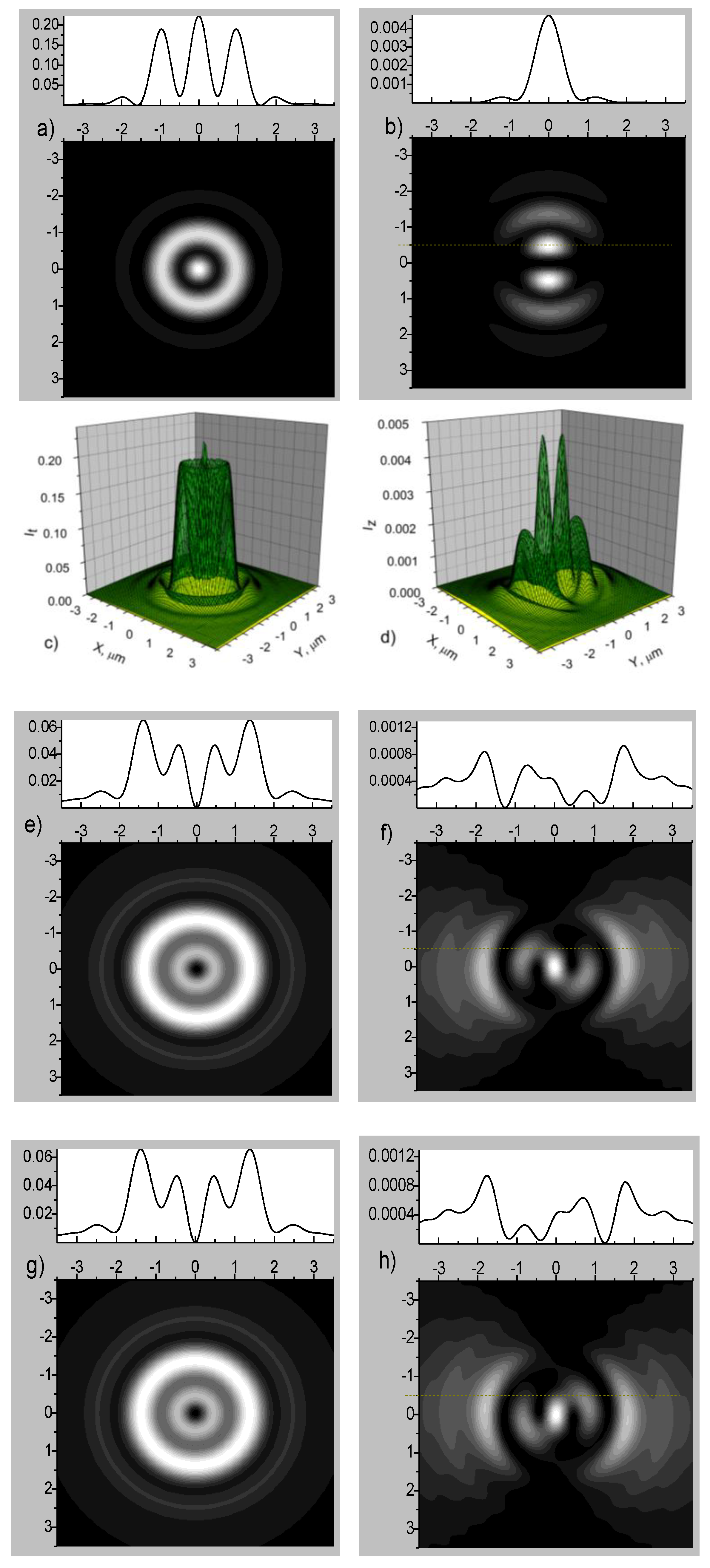
The intensity distribution changes with distance are determined by the functions and . Figure 8 shows the intensity distributions of the linearly polarized beams with the radial number and different OAMs in the focal plane. The gradient parameter of the medium (46) and the refractive index are considered. The beams with wavelength are considered. The numerical aperture is determined by , where a is the waveguide radius and . The initial beam width is . As can be seen, the intensity distributions depend on the SAM and OAM of the incident beam.
The focused spot in the longitudinal field is split into two equal parts if (Figure 8b). An asymmetry occurs between the intensity distributions of the longitudinal field component for incident beams with opposite OAM (Figure 8f,h). There is no such asymmetry for the transverse field components.
Note that the modes exhibiting hybrid entanglement between SAM and OAM may be useful for classical implementations of quantum communication and computational tasks [77].
3.2. The Splitting of the Degenerate Modes
In [23], the splitting of modes in a graded-index optical fiber due to the spin-orbit interaction is shown by solving the Maxwell equations using perturbation analysis. Due to the axial symmetry of the fiber, the modes are -fold degenerated, and for a given value of principal number , where and are the radial and azimuthal indices, the modes are degenerate by . The modes are -fold degenerated if the polarization degeneracy of the modes is taken into account.
The polarization degeneracy is eliminated by an additional term in the Hamiltonian describing the spin-orbit interaction. It is shown in [26] that the first order correction to the eigenvalue depends on the sign of the helicity and the total angular momentum
where , is the small parameter, is the total angular momentum, is the helicity, s is the spin angular momentum, and the longitudinal field component can be expressed through the transverse field components, i.e., .
The last term in (52) refers to the spin-orbit interaction and is analogous to the correction obtained for the modes of a ring resonator from a circular dielectric waveguide [78]. However, in their calculation results, the terms corresponding to the nonparaxiality were omitted. In fact, the first two terms in Equation (52) do not contribute to splitting a level with the same principal number and total angular momentum.
Using (49) the group delays of the modes are expressed by
where z is the length of the fiber, is the velocity of light in free space.
The group velocities of the vortex modes with right- and left-handed polarizations differ from each other, so the effective anisotropy is induced due to the spin-orbit interaction. In the case of zero orbital momentum, there is no such asymmetry.
3.3. Simulation of Delay Time and Group Delay Splitting
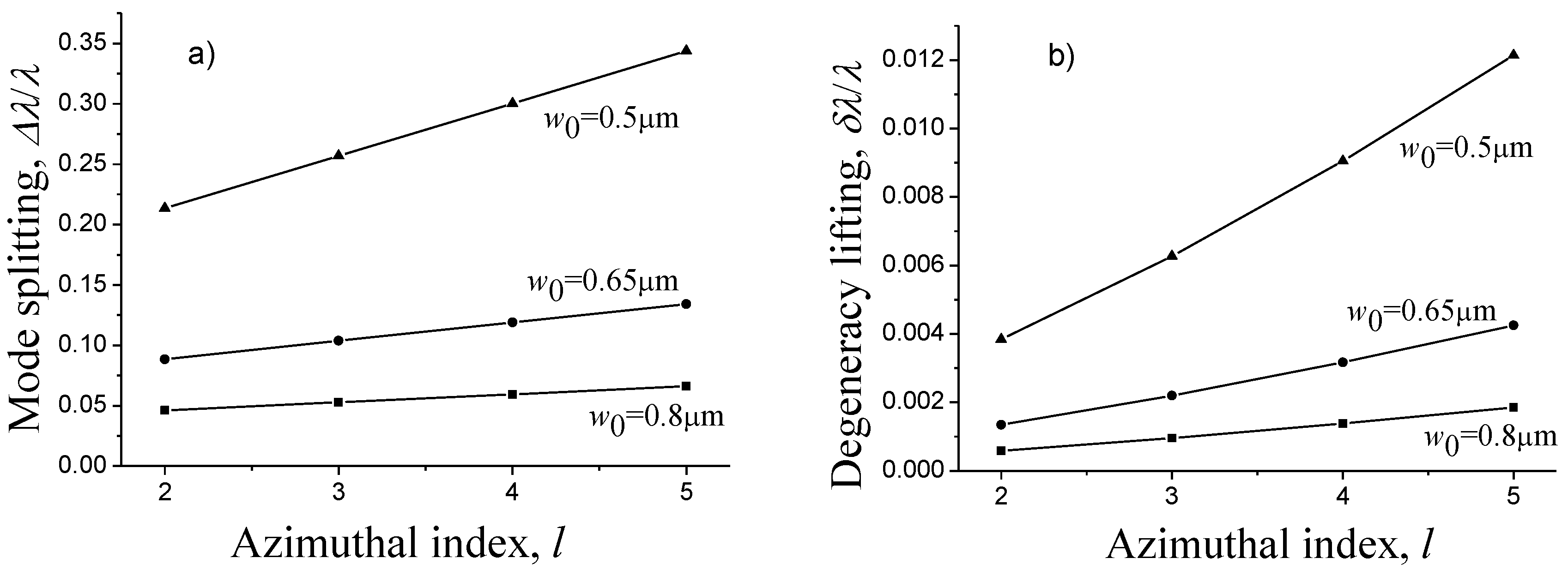
In Figure 9a the dependences of the propagation delay time of modes in comparison with the fundamental mode on the radial mode number for different fundamental mode radii are presented. In Figure 9b the group delay splitting of the azimuthal modes of fixed radial indices () is presented. It follows that the group delay splitting is an order of magnitude smaller than the relative propagation delay of modes.
Laguerre–Gauss beams are also modes of the Fabry–Perot resonator and fiber ring resonators made of a graded-index fiber. It follows from the resonance condition that the frequency shift and the corresponding wavelength shift are expressed by [26]:
where .
Note that the frequency shift of the same order of magnitude was obtained in [79,80]. In Figure 10a the wavelength shifts as a function of the azimuthal mode number for different beam radii are presented. The splitting is very sensitive to the size of the fundamental mode and increases with the azimuthal index. A similar result was obtained in almost hemispherical micro-cavities experimentally [81].
In addition to the polarization degeneracy, there is the degeneracy of modes with different orbital angular momentum and polarization, but with the same total angular momentum. In this case, corrections to the eigenvalues cannot be obtained from (52). The eigenvalues of the modes can be obtained analytically using the degenerate perturbation theory [26]:
There is a degeneracy lifting of the levels with the same total angular momentum j. The hybrid modes, which are solutions of Equation (44), correspond to these levels
The vector modes of a graded-index fiber are hybrid polarization-OAM-entangled states. Note that a similar OAM mixing of LG modes was also found in micro-cavities [82]. Because of the fact that the shift also takes place for the level with zero OAM, its mechanism is not only connected with the spin-orbit interaction, but also with nonparaxiality and tensor interaction [61]. The degeneracy lifting can be considered as an optical analogue of the Lamb shift, in which there is a separation of levels between degenerate states with the same total angular momentum.
The relative degeneracy lifting for different beam radii is shown in Figure 10b. The degeneracy lifting affects the quality Q-factor, which characterizes the resonant bandwidth of the modes. For resonators with the radius of the fundamental mode of the order of the wavelength of light, this splitting is about 1 nm, which can be observed experimentally.
3.4. Vector and Tensor Polarization Degrees of Light
The polarization state of the most general two-dimensional field can be fully described by three parameters. This is related to as vector polarization. For a three-dimensional field, in addition to the three components of the vector polarization, there are five components of tensor polarization.
Many works have been devoted to the description of the polarization of a three-dimensional field, in particular, several measures of the 3D degree of the polarization P have recently been proposed [83,84,85,86,87,88,89,90]. There is no unambiguous mathematical definition of the degree of polarization, that is, different measures of P are not equivalent, which indicates that a single parameter is not enough to fully describe all the properties of a three-dimensional field. The problem is that all measures of the 3D degree of polarization cannot distinguish between the two fields with different polarization matrices [84,85]. It is shown in [59] that two measures of the degrees of polarization (vector and tensor) are sufficient for a complete description of three-dimensional polarization, i.e., for distinguishing two fields with different polarization matrices. Examples illustrating various possible polarizing states are considered.
The elements of the Stokes vector are the intensity, vector and tensor polarizations which are defined in terms of the density matrix [61,62] (coherence matrix) ρ:
where are the spherical tensor operators, K = 1, 2; Q = 0, ±1, ±2.
Using the Equation (56) the density matrix may be written in terms of the expectation values tKQ:
where the scalar, vector and tensor components corresponding to monopole, dipole and quadrupole radiations are separately presented.
The spherical tensor operators in terms of components of the spin operator are [61,62]:
where , , , is the unit matrix and , .
The advantages of this representation are that these irreducible operators are transformed in the polarization space in the same way that spherical harmonics are transformed in the coordinate space [91], and that the measured light beam intensities can simply be expressed in terms of their mathematical expectations. The correspondence of the tensor elements to the field correlation components is easy to find from the expansion (57). Note that spherical operators can also be defined in terms of the Gell-Mann operators [58,59,83]. However, unlike the decomposition of three-dimensional fields onto Gell–Mann matrices, this decomposition has a physically clear interpretation.
The degree of polarization is described by the expression
It is reasonable to consider the vector and tensor polarization components in (59) separately, i.e., representing the total degree of polarization as [61]
where and are the vector and tensor polarization degrees, accordingly.
Vector polarization is defined by three parameters , , and the tensor polarization is defined by five parameters , , , and the normalization Trρ is not considered as a parameter. The values of Dv and Dt are determined by the possible values of the components t1Q and t2Q, which can be determined from the condition of positivity property of the diagonal elements of the density matrix (, , ), and the normalization condition for the total intensity.
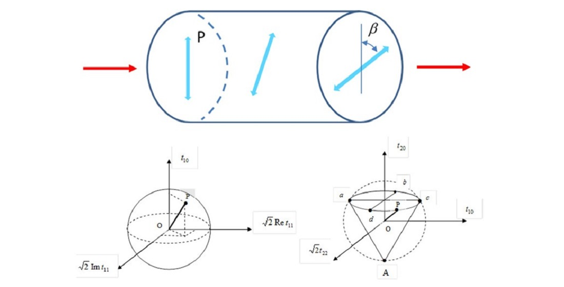
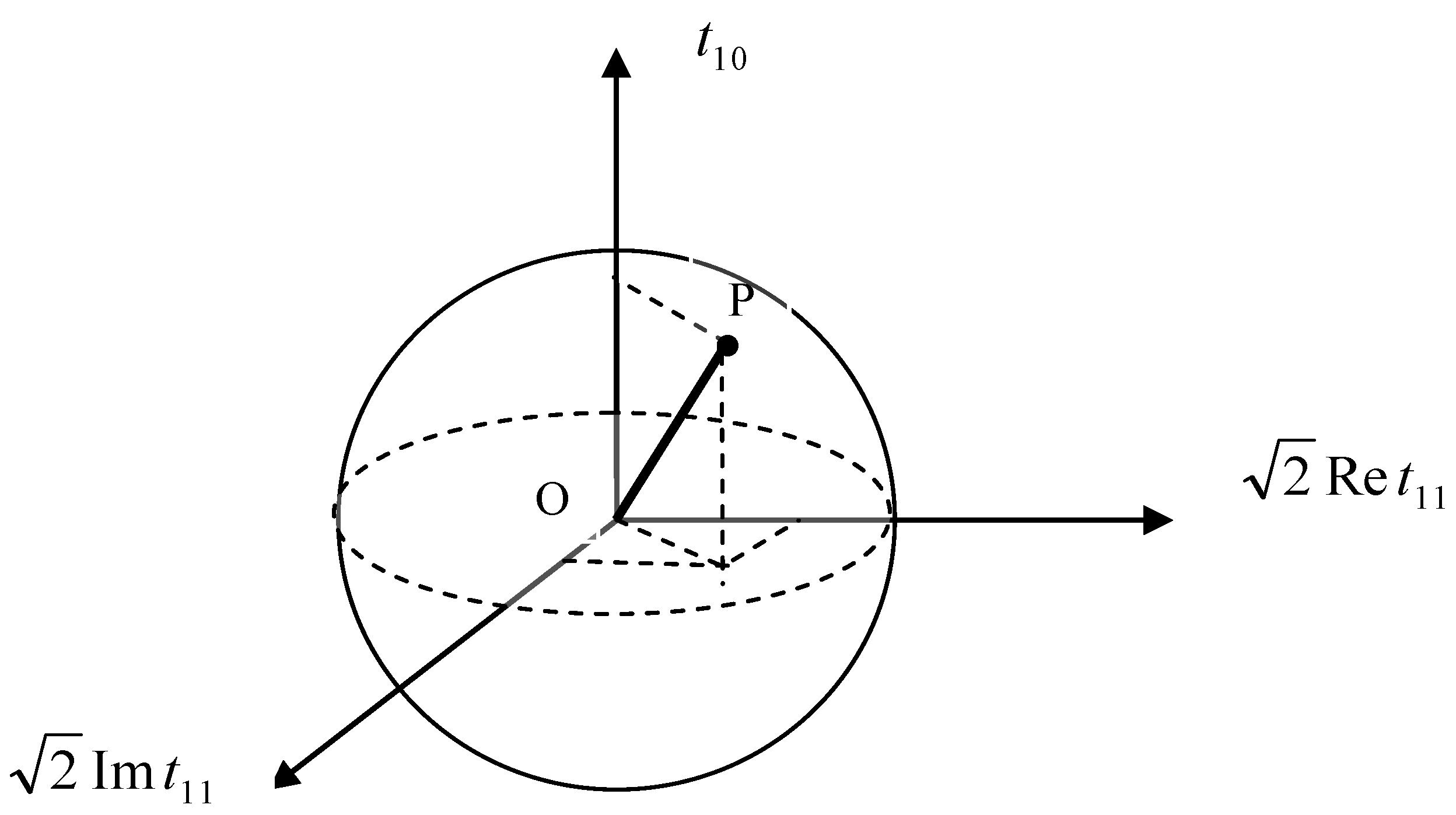
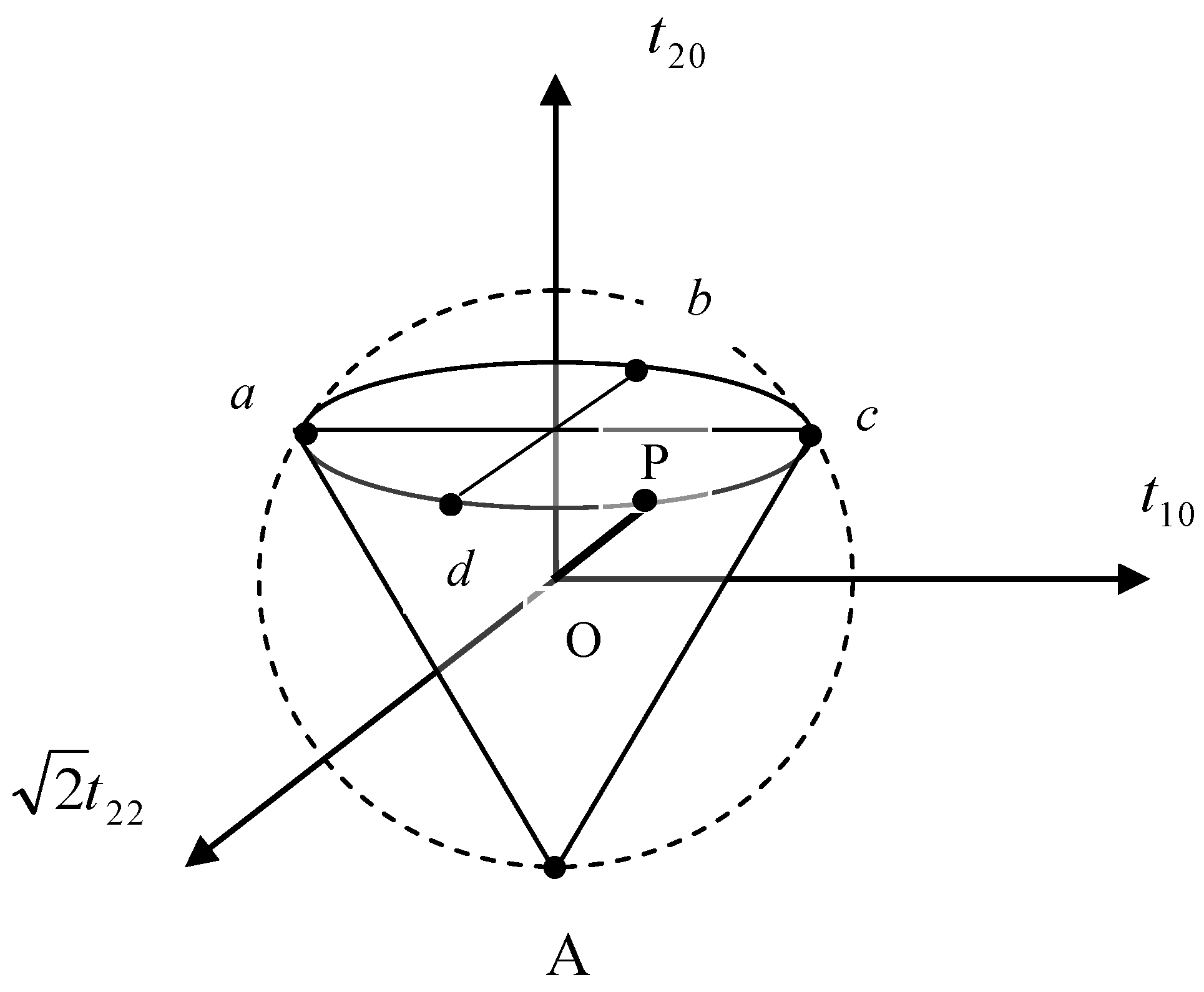
Geometrically, each possible vector polarization state can be represented by a point P in a sphere with radius of whose coordinates are , , and , respectively (Figure 11).
Acceptable values of the degree of vector polarization are , where Rv is the length of the vector OP (Figure 11). If we determine the vector polarization in the direction of the z-axis, the components disappear. In the case of the direction of the polarization vector along the principal axis of the symmetric second-rank tensor formed by , the components also disappear. The possible states of tensor polarization cannot be represented by a spherical area; these points form a cone inside a sphere with a radius of , and the permissible values of the degree of tensor polarization are (Figure 12).
The degree of polarization is determined by the length of the vector OP: , R = OP. Thus, the degree of polarization D < 1 for a pure vector polarized beam (Dt = 0), i.e., the vector polarized beam is only partially polarized (Figure 11). This indicates that it cannot be represented by a pure polarization state. However, there is a completely polarized beam that does not have a preferred direction of the polarization vector (), and this light beam is a pure tensor polarized beam (D = Dt = 1). This corresponds to the point at the top of the cone (point A in Figure 12). As can be seen from Figure 12, there are completely polarized states consisting of vector and tensor components of polarization on the circle abcd of the cone basis (for example, points a and c with and ). The points on the circle abcd correspond to circularly and linearly polarized beams and elliptically polarized states.
The unpolarized state of the beam is located in the center of the sphere. Note that in the 2D case, an unpolarized beam can be represented as the sum of two orthogonally (linearly or circularly) polarized beams, or as an incoherent mixture of equal amounts of two oppositely polarized beams. In the 3D case, an incoherent mixture of opposite polarization states and does not give a density matrix equal to the density matrix for an unpolarized beam [61]. The degree of polarization of this mixture is equal to . Moreover, the degrees of vector polarization for the pure state and the incoherent mixture of beams in the states and are equal to zero [61]. This means that vector polarization is not sufficient to completely determine the polarization state of a 3D light beam. Additional parameters (tensor polarization components) should be taken into account.
In the classical domain, there are nonzero intrinsic fluctuations of the Stokes parameters associated with tensor polarization components. Here, and . For an unpolarized light beam with the density matrix , the total fluctuations are equal to .
It can be shown that two parameters corresponding to the vector and tensor degrees of polarization are sufficient for a complete description of the characteristics of the electromagnetic field, i.e., to distinguish between the two fields with different polarization matrices. Let us consider two diagonalized polarization matrices ρ and with different eigenvalues () and (), respectively, having the same degrees of polarization . It is easy to demonstrate that and if only the matrices ρ and are identical, i.e., , , and . Indeed, the degrees of polarization for these fields are determined by the expressions [61]:
The condition of equality of the vector and tensor polarizations (, , ) leads to the equalities and . It can be seen that these equations are valid only in the case of , , and , i.e., two different density matrices cannot obey the condition , and , simultaneously. Thus, an unambiguous description of the polarization state of a light beam can be carried out using two parameters corresponding to the vector and tensor polarization degrees. Indeed, for the polarization matrices considered in [85], we have different vector and tensor polarization degrees for two different fields. For example, two density matrices with the eigenvalues λ1 = 0.7, λ2 = 0.2, λ3 = 0.1 and have the same values of the total degree of polarization D = 0.56. However, these matrices have different degrees of vector and tensor polarization: Dv = 0.52, Dt = 0.2, and 0.56, 0.0145, respectively.
To obtain a simple physical interpretation of the tensor polarization, it is useful to use the analogy between the polarization tensors and the multipole moments of the electrostatic potential generated by the distributed charge. It can be noted that the decomposition into irreducible representations of the rotation group SO(3) used above is actually a multipole decomposition [91]. The total intensity corresponds to an electric monopole, the vector polarization to an electric dipole, and the tensor polarization components to an electric quadrupole. However, there are limitations to the analogy with electric moments. If the electric dipole is a polar vector, then the polarization vector is an axial vector. Geometrically, tensor polarization can be represented by an ellipsoid of charge or an ellipsoid surface. In the case where one of the expectation values , , and disappears, the polarization tensor is represented by a degenerate ellipsoid, namely, a cylinder.
Note that the polarization ellipsoid associated with the polarization tensor is also analogous to the moment of inertia ellipsoid. The geometrical interpretation of the 3D polarization matrix in terms of the inertia ellipsoid and the orientation vector was considered in [88].
Since all the polarization components are associated with field correlations, the vector and tensor degrees of coherence corresponding to the vector and tensor parts of the density matrix decomposition can be introduced. In the far zone Ez → 0, and all tensor components of the second-rank are transformed into vector components. This means that the 2D formalism can be applied to describe the field in the far zone.
Thus, to describe an arbitrarily polarized light beam, the vector and tensor polarization degrees can be introduced. The representation in terms of vector and tensor operators allows us to obtain a simple physical insight into the proposed parameters for the polarization of an arbitrary field. It is shown that the tensor polarization components can be associated with the intrinsic fluctuations of the Stokes parameters. It is shown that for a complete description of three-dimensional polarization, two measures of the degrees of polarization (vector and tensor) are sufficient, i.e., to distinguish two different polarized fields. The proposed definition of polarization can be useful for describing electromagnetic fields in near field optics and analyzing propagation of a focused light beam.
4. Discussion
The polarization of electromagnetic waves play an important role in the interaction of light and matter, optical transmission, photonics, nanoplasmonics, high-power lasers and amplifiers, optical coherence tomography and imaging.
Multimode fibers are becoming important for improving the capabilities of next-generation telecommunication systems due to the spatial division multiplexing technique [92]. In recent years, they have attracted considerable attention in optical communication [93,94], soliton dynamics [95,96], ultrafast photonics [97,98], and other areas. In [99], the formation and manipulation of breathing solitons in graded-index multi-mode fibers was numerically demonstrated. Multimode fibers and nonlinear propagation within them can also be used to improve the efficiency of all optical data processing devices [100].
It was shown in [70] that classical beam propagation in optical waveguides can simulate quantum phenomena such as squeezing, Schrodinger cat states, collapse and revival. The possibility of measuring extremely small displacements, which can be used in laser gravitational-wave experiments and in ultra-high resolution spectroscopy, is shown. The results obtained can be useful in various fields, such as gravitational wave experiments, high-precision spectroscopy, and quantum information processing and metrology.
Due to the high mode dispersion, it is important to continuously analyze and monitor the dynamics of the modes propagating in multimode fibers. In [101], the complete polarization control of coherent light transmitted through an MMF with a strong mode and polarization coupling is experimentally demonstrated. It is necessary to propose a new measure of the degree of depolarization for simultaneous monitoring of the evolution of polarization. Recently, a new definition of the depolarization degree of partially polarized beams—the dispersion degree of polarization—has been proposed to measure the performance of fiber depolarizers [102].
It is of interest to determine the length of depolarization of light in real optical fibers. It is known [8,9,12] that when coherent light propagates in optical fibers, significant changes in the state and degree of polarization occur. As can be seen from Formulas (30) and (37), the degree of polarization depends on the gradient parameter of the fiber, the axial displacement x0 of the beam and the wavelength . From Equations (30) and (37), it is possible to determine that the depolarization length corresponds to a 50% decrease in the degree of polarization:
Substituting here the values for the gradient parameter µm−1 (a fiber with a radius r0 = x0 = 25 µm and a relative difference in the refractive index ) and the wavelength = 0.63 µm, we get the resulting distance cm. Such depolarization was experimentally observed in an isotropic multimode optical fiber [12]. Depolarization is enhanced by increasing the axial displacement of the incident beam or the angle of its inclination to the waveguide axis. Since rays with a large axial displacement x0 correspond to high-order fiber modes, the depolarization of modes with large numbers will be stronger compared to low-order modes. Therefore, in coherent communication systems, it is better to use single-mode fibers without birefringence, where the degree of polarization is retrieved with a period on propagation. This length in graded-index optical fibers is equal to 0.5 mm.
Note that the depolarization of light has a diffraction origin and the consideration of the Rytov rotation as a “geometric” depolarization mechanism is not correct. The Rytov rotation leads only to the rotation of the plane of polarization and not to a change in the degree of polarization. In addition, the angle of rotation of the polarization plane does not decrease with decreasing wavelength, whereas depolarization disappears at λ → 0. As shown above, depolarization also occurs for meridional rays for which there is no Rytov rotation.
Physically, depolarization corresponds to a decrease in the degree of correlation between different components of the field or to the appearance of a field component that is not correlated with the original component. In real situations, depolarization is most often caused by the scattering of light on small-scale inhomogeneities of the medium. The physical cause of depolarization in our case is the scattering of light on large-scale inhomogeneities of the medium. Since the influence of large-scale inhomogeneities on the polarization characteristics is small, it is usually neglected. However, in waveguide problems, small corrections accumulate with distance and can lead to noticeable effects.
Thus, the decrease in the degree of polarization in multimode optical fibers has a diffraction origin and can only be explained using the wave approach. Since depolarization disappears at both λ → 0 and x0 → 0, it can be interpreted as the result of the interaction of polarization (spin) and trajectory (orbital angular momentum). The degree of polarization of both linearly and circularly polarized beams decreases with distance according to the quadratic law. The depolarization of the meridional rays is less than that of the sagittal rays. For right- and left-handed circularly polarized light, the effect of asymmetry with respect to the sign of the twist of the sagittal ray trajectory is observed. Depolarization is enhanced by increasing the axial displacement of the beam, the gradient parameter of the fiber and the radiation wavelength.
For three-dimensional polarization, the coherence matrix of three-dimensional electromagnetic fields is represented as spherical or rectangular tensors, similar to the Gell–Mann matrices. The evolution of the coherency matrix can be defined in terms of the Hamiltonian obtained from the three-component field Maxwell equations. It is shown that two measures of the degrees of polarization (vector and tensor) are sufficient for a complete description of the three-dimensional polarization, that is, for distinguishing two fields with different polarization matrices [61]. The paper [59] shows the possibility of an unambiguous description of three-dimensional polarization using two measures, namely, the vector and tensor degrees of polarization. Note that the polarization matrix of any three-dimensional field can be directly measured using nanoprobe scatterers [103,104], which enables an experimental determination of the vector and tensor degrees of polarization of the light under consideration.
Finally, we present the fundamental effect of spin symmetry breaking via spin-orbit and tensor interactions, which occurs even in rotationally symmetric fibers. Due to this effect, the conversion of the incident linear polarized light into a particularly left- or right-handed circularly polarized light can be achieved. Although the effect manifests itself in a graded-index fiber, it manifests itself in general cylindrical potentials, in particular the Coulomb cylindrical potential. The phenomenon can be used in polarization control applications, such as new circular polarizers, polarization transformers and modulators.
Recently, new developments in the phenomenon known as transverse spin, which occurs in laterally confined electromagnetic waves, have been of great interest [105]. The spin-pulse blocking effect associated with transverse spin has already found promising applications for efficient spin-directed couplers [106,107].
More recently, interesting optical phenomena related to the angular momentum of light have been demonstrated theoretically and experimentally [108,109,110]. In [109], vectorial optomechanical effects mediated by the anisotropy of a nematic liquid crystal material and the longitudinal field component were discovered. It was shown in [108] that transverse spin is essentially a polarization-independent phenomenon that persists even in fields generated by completely unpolarized sources. The transverse spin appears in any paraxial-to-nonparaxial transformation, even without a change in the degree of polarization. This result establishes an important connection between three-dimensional polarization in the transverse spin [103,111] and non-paraxial fields [58,59,60,61,112,113]. The origin of this phenomenon lies in the intrinsic spin-orbit interaction of light. These results provide a new opportunity to use polarization-independent spin from unpolarized sources, such as in nanoelectronics, telecommunications, photovoltaics, optical imaging, etc. Transverse spin can also be useful for unidirectional coupling of light in and from optical fibers or waveguides, which may have implications for future quantum networks [114,115].
5. Conclusions
In this review, we focused on studying the effects of spin-orbit interactions in the propagation of vortex light through multimode graded-index fibers. Several detailed examples discussed in this review demonstrate that optical fibers supporting vortex beams can be considered using an operator approach well-developed in quantum mechanics. With this approach, all the dynamics of the system are transferred to the operators. This makes it possible to study the evolution of the beam parameters using purely algebraic procedures, i.e., without using explicit expressions for the wave functions of the field and without calculating the corresponding integrals. This model is simple and provides a physical clarification of the phenomenon. Note that the operator approach can be used to study the evolution of polarization in optical fibers with birefringence, absorption, or amplification, as well as with random inhomogeneities.
Understanding the relationship between the degree of polarization, the spin-orbit interaction and the Berry phase is important for the design of optical devices, such as new polarizers, polarization transformers, and modulators. Fluctuations of the Berry’s phase, which have a wave nature, during the propagation of light in an optical fiber were found in [57]. It was shown that the variance of the rotation angle of the polarization plane increases with distance and can be determined by measuring the degree of polarization.
Spin-dependent effects on vortex light beams propagating in an optical fiber are demonstrated by solving the full three-component field Maxwell equations using perturbation analysis. The splitting of degenerate modes due to the spin-orbit interaction is shown. Vector and tensor polarization degrees are introduced to characterize the polarized beam. It is shown that the degree of the pure vector polarized light beam is less than 1, that is, the vector polarized light beam is only partially polarized. The geometric interpretation of vector and tensor polarizations is presented.
Funding
The reported study was funded by the Russian Foundation for Basic Research, project number 19-29-11026 and the Ministry of Science and Higher Education of the Russian Federation under the State contract No. 0069-2019-0006.
Institutional Review Board Statement
Not applicable.
Informed Consent Statement
Not applicable.
Data Availability Statement
Not applicable.
Conflicts of Interest
The author declares no conflict of interest.
References
- Azzam, R.M.A.; Bashara, N.M. Ellipsometry and Polarized Light; North-Holland: Amsterdam, The Netherlands, 1977. [Google Scholar]
- Wolf, E. Introduction to the Theory of Coherence and Polarization of Light; Cambridge University Press: Cambridge, UK, 2007. [Google Scholar]
- Tatarskii, V.I. Estimation of light depolarization by turbulent inhomogeneities of the atmosphere. Izv. VUZov Radiofiz. 1967, 10, 1762–1765. [Google Scholar]
- Kravtzov, Y.A. Geometrical depolarization of light in a turbulent atmosphere. Izv. VUZov Radiofiz. 1970, 13, 281–284. [Google Scholar]
- Rytov, S.M. On transition from wave to geometrical optics. Dokl. Akad. Nauk USSR 1938, 18, 263–266. [Google Scholar]
- Vladimirsky, V.V. On rotation of polarization plane in twisted ray of light. Dokl. Akad. Nauk USSR 1941, 31, 222–225. [Google Scholar]
- Cohen, L.G. Measured attenuation and depolarization of light transmitted along glass fibers. Bell Syst. Tech. J. 1971, 50, 23–42. [Google Scholar] [CrossRef]
- Smith, A.M. Polarization and magnetooptic properties of single-mode optical fiber. Appl. Opt. 1978, 17, 52–56. [Google Scholar] [CrossRef] [PubMed]
- Kaminov, I.P. Polarization in optical fibers. IEEE J. Quant. Electron. 1981, 17, 15–22. [Google Scholar] [CrossRef]
- Shatrov, A.D. Polarization effects in multimode graded-index fibers. Radiotekh. Elektr. 1988, 26, 505–512. [Google Scholar]
- Esayan, A.A.; Zel’dovich, B.Y. Depolarization of radiation in an ideal multimode graded-index optical fiber. Soviet J. Quantum Electron. 1988, 18, 149–150. [Google Scholar] [CrossRef]
- Kotov, O.I.; Marusov, O.L.; Nikolaev, O.L.; Filippov, V.N. Polarization properties of optical fibers. Modal approach. Opt. Spectr. 1991, 70, 924–927. [Google Scholar]
- Zel’dovich, B.Y.; Kundikova, N.D. Intrafibre rotation of the plane of polarization. Quantum Electron. 1995, 25, 172–174. [Google Scholar] [CrossRef]
- Zel’dovich, B.Y.; Liberman, V.S. Rotation of the plane of a meridional beam in a graded-index waveguide due to the circular nature of the polarization. Soviet J. Quantum Electron. 1990, 20, 427–428. [Google Scholar] [CrossRef]
- Zel’dovich, B.Y.; Kitaevskaya, I.V.; Kundikova, I.D. Inhomogeneity of the optical Magnus effect. Quantum Electron. 1996, 26, 87–88. [Google Scholar] [CrossRef]
- Petrov, N.I. Depolarization of light in a graded-index isotropic medium. J. Mod. Opt. 1996, 43, 2239–2249. [Google Scholar] [CrossRef]
- Petrov, N.I. Evolution of polarization in an inhomogeneous isotropic medium. JETP 1997, 85, 1085–1093. [Google Scholar] [CrossRef]
- Matthews, S.C.; Rockwell, D.A. Correction of phase and depolarization distortions in a multimode fiber at 1.064 μm with stimulated-Brillouin-scattering phase conjugation. Opt. Lett. 1994, 19, 1729–1731. [Google Scholar] [CrossRef] [PubMed]
- Roychowdhury, H.; Agrawal, G.P.; Wolf, E. Changes in the spectrum, in the spectral degree of polarization, and in the spectral degree of coherence of a partially coherent beam propagating through a gradient-index fiber. J. Opt. Soc. Am. A 2006, 23, 940–948. [Google Scholar] [CrossRef] [PubMed]
- Huang, W.; Ponomarenko, S.A.; Cada, M.; Agrawal, G.P. Polarization changes of partially coherent pulses propagating in optical fibers. JOSA A 2007, 24, 3063–3068. [Google Scholar] [CrossRef] [PubMed]
- Bliokh, K.Y.; Desyatnikov, A.S. Spin and orbital Hall effects for diffracting optical beams in gradient-index media. Phys. Rev. A 2009, 79, 011807. [Google Scholar] [CrossRef] [Green Version]
- Bliokh, K.Y. Geometrodynamics of polarized light: Berry phase and spin Hall effect in a gradient-index medium. J. Opt. A Pure Appl. Opt. 2009, 11, 094009. [Google Scholar] [CrossRef] [Green Version]
- Chakravarthy, T.P.; Viswanatham, N.K. Direct and reciprocal spin-orbit interaction effects in a graded-index medium. OSA Contin. 2019, 2, 1576–1589. [Google Scholar] [CrossRef]
- Dugin, A.; Zel’dovich, B.; Kundikova, N.; Liberman, V. Effect of circular polarization on the propagation of light through an optical fiber. J. Exp. Theor. Phys. Lett. 1991, 53, 197–199. [Google Scholar]
- Petrov, N.I. Evolution of 3D Polarization in Inhomogeneous Medium. In Proceedings of the Frontiers in Optics 2007, San Jose, CA, USA, 16–20 September 2007. [Google Scholar] [CrossRef]
- Petrov, N.I. Splitting of levels in a cylindrical dielectric waveguide. Opt. Lett. 2013, 38, 2020–2022. [Google Scholar] [CrossRef] [PubMed] [Green Version]
- Petrov, N.I. Spin-dependent transverse force on a vortex light beam in an inhomogeneous medium. JETP Lett. 2016, 103, 443–448. [Google Scholar] [CrossRef]
- Petrov, N.I. Vector Laguerre–Gauss beams with polarization-orbital angular momentum entanglement in a graded-index medium. J. Opt. Soc. Am. A 2016, 33, 1363–1369. [Google Scholar] [CrossRef] [PubMed] [Green Version]
- Arnaud, J.A. Beam and Fiber Optics; Academic Press: New York, NY, USA, 1976. [Google Scholar]
- Tomita, A.; Chiao, R.Y. Observation of Berry’s Topological Phase by Use of an Optical Fiber. Phys. Rev. Lett. 1986, 57, 937–940. [Google Scholar] [CrossRef] [PubMed] [Green Version]
- Berry, M.V. Quantal phase factors accompanying adiabatic changes. Proc. R. Soc. Lond. A 1984, 392, 45–57. [Google Scholar]
- Imbert, C. Calculation and experimental proof of the transverse shift induced by total internal reflection of a circularly polarized light beam. Phys. Rev. D 1972, 5, 787–796. [Google Scholar] [CrossRef]
- Goos, F.; Hanchen, H. Ein neuer und fundamentaler versuch zur total reflexion. Ann. Phys. 1947, 1, 333–345. [Google Scholar] [CrossRef] [Green Version]
- Petrov, N.I. Reflection and transmission of strongly focused light beams at a dielectric interface. J. Mod. Opt. 2005, 52, 1545–1556. [Google Scholar] [CrossRef]
- Petrov, N.I. The influence of polarization on the trajectory and the width of a radiation beam in an inhomogeneous medium. Las. Phys. 2000, 10, 619–621. [Google Scholar]
- Bliokh, K.Y.; Niv, A.; Kleiner, V.; Hasman, E. Geometrodynamics of spinning light. Nat. Photon. 2008, 2, 748–753. [Google Scholar] [CrossRef]
- Liberman, V.S.; Zel’dovich, B.Y. Spin-orbit interaction of a photon in an inhomogeneous medium. Phys. Rev. A 1992, 46, 5199–5207. [Google Scholar] [CrossRef] [PubMed]
- Onoda, M.; Murakami, S.; Nagaosa, N. Hall Effect of Light. Phys. Rev. Lett. 2004, 93, 083901. [Google Scholar] [CrossRef] [PubMed] [Green Version]
- Kavokin, A.; Malpuech, G.; Glazov, M. Optical Spin Hall Effect. Phys. Rev. Lett. 2005, 95, 136601. [Google Scholar] [CrossRef] [PubMed] [Green Version]
- Snyder, A.W.; Love, J.D. Optical Waveguide Theory; Chapman and Hall: London, UK, 1983. [Google Scholar]
- Sodha, M.S.; Ghatak, A.K. Inhomogeneous Optical Waveguides; Plenum Press: New York, NY, USA, 1977. [Google Scholar]
- Loffler, W.; Van Exter, M.P.; Hooft, G.W.; Eliel, E.R.; Hermans, K.; Broer, D.J.; Woerdman, J.P. Polarization-dependent Goos–Hänchen shift at a graded dielectric interface. Opt. Commun. 2010, 283, 3367–3370. [Google Scholar] [CrossRef]
- Petrov, N.I. Beam shift in a graded-index optical fiber. J. Opt. 2013, 15, 014011. [Google Scholar] [CrossRef]
- Glauber, R.J. Coherent and Incoherent States of the Radiation Field. Phys. Rev. 1963, 131, 2766–2788. [Google Scholar] [CrossRef]
- Schrodinger, E. Der stetige Übergang von der Mikro-zur Makromechanik. Naturwissenschaften 1926, 14, 664–666. [Google Scholar] [CrossRef]
- Krivoshlykov, S.G.; Sissakian, I.N. Coherent states and light propagation in inhomogeneous media. Soviet J. Quantum Electron. 1980, 10, 312–318. [Google Scholar] [CrossRef]
- Krivoshlykov, S.G.; Petrov, N.I.; Sisakyan, I.N. Density-matrix formalism for partially coherent optical fields propagating in slightly inhomogeneous media. Opt. Quant. Electr. 1986, 18, 253–264. [Google Scholar] [CrossRef]
- Petrov, N.I.; Petrova, G.N. Diffraction of partially-coherent light beams by microlens arrays. Opt. Exp. 2017, 25, 22545–22564. [Google Scholar] [CrossRef] [PubMed]
- Hansson, T.; Tonello, A.; Mansuryan, T.; Mangini, F.; Zitelli, M.; Ferraro, M.; Niang, A.; Crescenzi, R.; Wabnitz, S.; Couderc, V. Nonlinear beam self-imaging and self-focusing dynamics in a GRIN multimode optical fiber: Theory and experiments. Opt. Exp. 2020, 16, 24005–24021. [Google Scholar] [CrossRef] [PubMed]
- Mangini, F.; Ferraro, M.; Zitelli, M.; Niang, A.; Tonello, A.; Couderc, V.; Sidelnikov, O.; Frezza, F.; Wabnitz, S. Experimental observation of self-imaging in SMF-28 optical fibers. Opt. Exp. 2021, 8, 12625–12633. [Google Scholar] [CrossRef] [PubMed]
- Merano, M.; Hermosa, N.; Aiello, A.; Woerdman, J.P. Demonstration of a quasi-scalar angular Goos–Hänchen effect. Opt. Lett. 2010, 35, 3562–3564. [Google Scholar] [CrossRef] [PubMed]
- Petrov, N.I.; Danilov, V.A.; Popov, V.V.; Usievich, B.A. Large positive and negative Goos-Hänchen shifts near the surface plasmon resonance in subwavelength grating. Opt. Exp. 2020, 28, 7552–7564. [Google Scholar] [CrossRef] [PubMed]
- Petrov, N.I. Focusing of beams into subwavelength area in an inhomogeneous medium. Opt. Exp. 2001, 9, 658–673. [Google Scholar] [CrossRef] [PubMed]
- Petrov, N.I. Remote focusing of a light beam. Las. Phys. Lett. 2016, 13, 015101. [Google Scholar] [CrossRef] [Green Version]
- Tychinskii, V.P. Microscopy of subwavelength structures. Phys. Uspekhi 1996, 39, 1157–1167. [Google Scholar] [CrossRef]
- Sato, M.; Eto, K.; Masuta, J.; Nishidate, I. Depolarization characteristics of spatial modes in imaging probe using short multimode fiber. Appl. Opt. 2018, 57, 10083–10091. [Google Scholar] [CrossRef] [PubMed]
- Petrov, N.I. Evolution of Berry’s phase in a graded-index medium. Phys. Lett. A 1997, 234, 239–250. [Google Scholar] [CrossRef]
- Carozzi, T.; Karlsson, R.; Bergman, J. Parameters characterizing electromagnetic wave polarization. Phys. Rev. E 2000, 61, 2024–2028. [Google Scholar] [CrossRef] [PubMed] [Green Version]
- Setala, T.; Shevchenko, A.; Kaivola, M.; Friberg, A.T. Degree of polarization for optical near fields. Phys. Rev. E 2002, 66, 016615. [Google Scholar] [CrossRef] [PubMed] [Green Version]
- Dennis, M.R. Geometric interpretation of the three-dimensional coherence matrix for nonparaxial polarization. Pure Appl. Opt. 2004, 6, S26–S31. [Google Scholar] [CrossRef]
- Petrov, N.I. Vector and tensor polarizations of light beams. Laser Phys. 2008, 18, 522–525. [Google Scholar] [CrossRef]
- Petrov, N.I. Spin-orbit and tensor interactions of light in inhomogeneous isotropic media. Phys. Rev. A 2013, 88, 023815. [Google Scholar] [CrossRef]
- Feit, M.D.; Fleck, J.A. Light propagation in graded-index optical fibers. Appl. Opt. 1978, 17, 3990–3998. [Google Scholar] [CrossRef] [PubMed]
- Krivoshlykov, S.G.; Sisakyan, I.N. Coherent states and nonparaxial propagation of light in graded-index media. Soviet J. Quantum Electron. 1983, 13, 455–458. [Google Scholar] [CrossRef]
- Petrov, N.I. Physico-Mathematical Sciences. Ph.D. Thesis, General Physics Institute, Russian Academy of Sciences, Moscow, Russia, 1985. [Google Scholar]
- Krivoshlykov, S.G.; Petrov, N.I.; Sissakian, I.N. Correlated coherent states and propagation of arbitrary Gaussian beams in longitudinally homogeneous quadratic media exhibiting absorption or amplification. Soviet J. Quantum Electron. 1986, 16, 933–941. [Google Scholar] [CrossRef]
- Krivoshlykov, S.G. Non-paraxial propagation of Gaussian beam rays in graded-index waveguides and effect of large-scale initial field revival. J. Mod. Opt. 1992, 39, 723–736. [Google Scholar] [CrossRef]
- Petrov, N.I. Mode structure formation length in an inhomogeneous medium. Laser Phys. 1998, 8, 1245–1248. [Google Scholar]
- Petrov, N.I. Nonparaxial focusing of wave beams in a graded-index medium. Quantum Electron. 1999, 29, 249–255. [Google Scholar] [CrossRef]
- Petrov, N.I. Macroscopic quantum effects for classical light. Phys. Rev. A 2014, 90, 043814. [Google Scholar] [CrossRef] [Green Version]
- Arrizon, V.; Soto-Eguibar, F.; Zuniga-Segundo, A.; Moya-Cessa, H.M. Revival and splitting of a Gaussian beam in gradient index media. JOSA A 2015, 32, 1140. [Google Scholar] [CrossRef] [PubMed] [Green Version]
- Karimi, E.; Santamoto, E. Radial coherent and intelligent states of paraxial wave equation. Opt. Lett. 2012, 37, 2484. [Google Scholar] [CrossRef] [PubMed] [Green Version]
- Hermoza, N.; Aiello, A.; Woerdman, J.P. Radial mode dependence of optical beam shifts. Opt. Lett. 2012, 37, 1044. [Google Scholar] [CrossRef] [Green Version]
- Plick, W.N.; Lapkiewicz, R.; Ramelow, S.; Zeilinger, A. The Forgotten Quantum Number: A short note on the radial modes of Laguerre-Gauss beams. arXiv 2013, arXiv:1306.6517. [Google Scholar]
- Petrov, N.I. Speed of structured light pulses in free space. Sci. Rep. 2019, 9, 18332. [Google Scholar] [CrossRef] [PubMed]
- Petrov, N.I. Evanescent and propagating fields of strongly focused beams. JOSA A 2003, 20, 2385–2389. [Google Scholar] [CrossRef] [PubMed]
- Barreiro, J.T.; Wei, T.C.; Kwiat, P.G. Remote Preparation of Single-Photon “Hybrid” Entangled and Vector-Polarization States. Phys. Rev. Lett. 2010, 105, 030407. [Google Scholar] [CrossRef] [PubMed] [Green Version]
- Bliokh, K.Y.; Frolov, D.Y. Spin-orbit interaction of photons and fine splitting of levels in ring dielectric resonator. Opt. Commun. 2005, 250, 321–327. [Google Scholar] [CrossRef] [Green Version]
- Erickson, C.W. High order modes in a spherical Fabry-Perot resonator. IEEE Trans. Microw. Theory Tech. 1975, 23, 218–223. [Google Scholar] [CrossRef]
- Yu, P.K.; Luk, K. Field patterns and resonant frequencies of high-order modes in an open resonator. IEEE Trans. Microw. Theory Tech. 1984, 32, 641–645. [Google Scholar]
- Pennington, R.C.; Alessandro, G.D.; Baumberg, J.J.; Kaczmarek, M. Tracking spatial modes in nearly hemispherical microcavities. Opt. Lett. 2007, 32, 3131–3133. [Google Scholar] [CrossRef] [PubMed]
- Foster, D.H.; Nockel, J.U. Bragg-induced orbital angular-momentum mixing in paraxial high-finesse cavities. Opt. Lett. 2004, 29, 2788–2790. [Google Scholar] [CrossRef] [PubMed] [Green Version]
- Brosseau, C. Entropy and Polarization of a Stochastic Radiation Field. Prog. Quantum Electron. 1997, 21, 421–461. [Google Scholar] [CrossRef]
- Ellis, J.; Dogariu, A.; Ponomarenko, S.; Wolf, E. Degree of polarization of statistically stationary electromagnetic fields. Opt. Commun. 2005, 248, 333–337. [Google Scholar] [CrossRef]
- Ellis, J.; Dogariu, A. On the degree of polarization of random electromagnetic fields. Opt. Commun. 2005, 253, 257–265. [Google Scholar] [CrossRef]
- Dennis, M.R. A three-dimensional degree of polarization based on Rayleigh scattering. J. Opt. Soc. Am. A 2007, 24, 2065–2069. [Google Scholar] [CrossRef] [PubMed] [Green Version]
- Petruccelli, J.C.; Moore, N.J.; Alonso, M.A. Two methods for modeling the propagation of the coherence and polarization properties of nonparaxial fields. Opt. Commun. 2010, 283, 4457–4466. [Google Scholar] [CrossRef]
- Sheppard, C.J.R. Jones and Stokes parameters for polarization in three dimensions. Phys. Rev. A 2014, 90, 023809. [Google Scholar] [CrossRef]
- Gil, J.J. Intrinsic Stokes parameters for 3D and 2D polarization states. J. Eur. Opt. Soc. Rapid 2015, 10, 15054. [Google Scholar] [CrossRef] [Green Version]
- Gil, J.J.; Norman, A.; Friberg, A.T.; Setala, T. Polarimetric purity and the concept of degree of polarization. Phys. Rev. A 2018, 97, 023838. [Google Scholar] [CrossRef] [Green Version]
- Arfken, G.B.; Weber, H.J. Mathematical Methods for Physicists; Elsevier: Amsterdam, The Netherlands, 2005. [Google Scholar]
- Richardson, D.J.; Fini, J.M.; Nelson, L.E. Space-division multiplexing in optical fibres. Nat. Photon. 2013, 7, 354–362. [Google Scholar] [CrossRef] [Green Version]
- Stuart, H.R. Dispersive multiplexing in multimode optical fiber. Science 2000, 289, 281–283. [Google Scholar] [CrossRef] [PubMed]
- Tzang, O.; Caravaca-Aguirre, A.M.; Wagner, K.; Piestun, R. Adaptive wavefront shaping for controlling nonlinear multimode interactions in optical fibres. Nat. Photon. 2018, 12, 368–374. [Google Scholar] [CrossRef]
- Wright, L.G.; Renninger, W.H.; Christodoulides, D.N.; Wise, F.W. Spatiotemporal dynamics of multimode optical solitons. Opt. Exp. 2015, 23, 3492–3506. [Google Scholar] [CrossRef] [PubMed]
- Wright, L.G.; Christodoulides, D.N.; Wise, F.W. Controllable spatiotemporal nonlinear effects in multimode fibres. Nat. Photon. 2015, 9, 306–310. [Google Scholar] [CrossRef]
- Fu, W.; Wright, L.G.; Sidorenko, P.; Backus, S.; Wise, F.W. Several new directions for ultrafast fiber lasers [Invited]. Opt. Express 2018, 26, 9432–9463. [Google Scholar] [CrossRef] [PubMed]
- Wright, L.G.; Christodoulides, D.N.; Wise, F.W. Spatiotemporal mode-locking in multimode fiber lasers. Science 2017, 358, 94–97. [Google Scholar] [CrossRef] [PubMed] [Green Version]
- Deng, Z.; Chen, Y.; Liu, J.; Zhao, C.; Fan, D. Graded-index breathing solitons from Airy pulses in multimode fibers. Opt. Exp. 2019, 27, 483–493. [Google Scholar] [CrossRef] [PubMed]
- Krupa, K.; Tonello, A.; Barthélémy, A.; Mansuryan, T.; Couderc, V.; Millot, G.; Grelu, P.; Modotto, D.; Babin, S.A.; Wabnitz, S. Multimode nonlinear fiber optics, a spatiotemporal avenue. APL Photon. 2019, 4, 110901. [Google Scholar] [CrossRef]
- Xiong, W.; Hsu, C.W.; Bromberg, Y.; Antonio-Lopez, J.E.; Correa, R.A.; Cao, H. Complete polarization control in multimode fibers with polarization and mode coupling. Light Sci. Appl. 2018, 7, 54. [Google Scholar] [CrossRef] [PubMed] [Green Version]
- Zou, K.; Miao, L.; Wang, G.; Bi, R.; Chen, K.; She, X.; Shu, X. Light depolarization based on dispersion degree of polarization. Appl. Opt. 2020, 59, 11301–11309. [Google Scholar] [CrossRef] [PubMed]
- Ellis, J.; Dogariu, A. Optical Polarimetry of Random Fields. Phys. Rev. Lett. 2005, 95, 203905. [Google Scholar] [CrossRef] [PubMed]
- Leppänen, A.L.P.; Friberg, T.; Setälä, T. Partial polarization of optical beams and near fields probed with a nanoscatterer. J. Opt. Soc. Am. A 2014, 31, 1627–1635. [Google Scholar] [CrossRef] [PubMed]
- Bliokh, K.Y.; Nori, F. Transverse and longitudinal angular momenta of light. Phys. Rep. 2015, 592, 1–38. [Google Scholar] [CrossRef] [Green Version]
- Petersen, J.V.; Rauschenbeutel, A. Chiral nano-photonic waveguide interface based on spin-orbit interaction of light. Science 2014, 346, 67–71. [Google Scholar] [CrossRef] [PubMed] [Green Version]
- Lefier, Y.; Grosjean, T. Unidirectional sub-diffraction waveguiding based on optical spin-orbit coupling in subwavelength plasmonic waveguides. Opt. Lett. 2015, 40, 2890–2893. [Google Scholar] [CrossRef]
- Eismann, J.S.; Nicholls, L.H.; Roth, D.J.; Alonso, M.A.; Banzer, P.; Rodríguez-Fortuño, F.J.; Zayats, A.V.; Nori, F.; Bliokh, K.Y. Transverse spinning of unpolarized light. Nat. Photon. 2020, 15, 156–161. [Google Scholar] [CrossRef]
- Ketara, M.L.; Kobayashi, H.; Brasselet, E. Sensitive vectorial optomechanical footprint of light in soft condensed matter. Nat. Photon. 2021, 15, 121–124. [Google Scholar] [CrossRef]
- Cardano, F.; Marrucci, L. Longitudinal fields and transverse rotations. Nat. Photon. 2021, 15, 72–74. [Google Scholar] [CrossRef]
- Golat, S.; Lim, E.A.; Rodríguez-Fortuño, F.J. Evanescent Gravitational Waves. arXiv 2020, arXiv:1903.09690. [Google Scholar] [CrossRef]
- Lindfors, K.; Setälä, T.; Kaivola, M.; Friberg, A.T. Degree of polarization in tightly focused optical fields. J. Opt. Soc. Am. A 2005, 22, 561–568. [Google Scholar] [CrossRef] [PubMed] [Green Version]
- Lindfors, K.; Priimagi, A.; Setälä, T.; Shevchenko, A.; Friberg, A.T.; Kaivola, M. Local polarization of tightly focused unpolarized light. Nat. Photon. 2007, 1, 228–231. [Google Scholar] [CrossRef]
- Marrucci, L. Spin gives direction. Nat. Photon. 2014, 11, 9–10. [Google Scholar] [CrossRef] [Green Version]
- Wang, J.; Sciarrino, F.; Laing, A.; Thomson, M.G. Integrated photonic quantum technologies. Nat. Photon. 2020, 14, 273–284. [Google Scholar] [CrossRef]
Figure 1.
Dependence of the angular GH shift on the diffraction angular divergence of the beam.
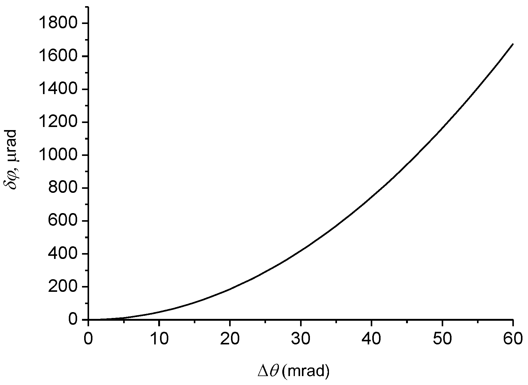
Figure 2.
The degree of linear polarization as a function of distance for both meridional and sagittal rays (solid curves) and only for meridional rays (dashed curves). (1) x0 = 15 μm; (2) x0 = 5 μm.
Figure 2.
The degree of linear polarization as a function of distance for both meridional and sagittal rays (solid curves) and only for meridional rays (dashed curves). (1) x0 = 15 μm; (2) x0 = 5 μm.
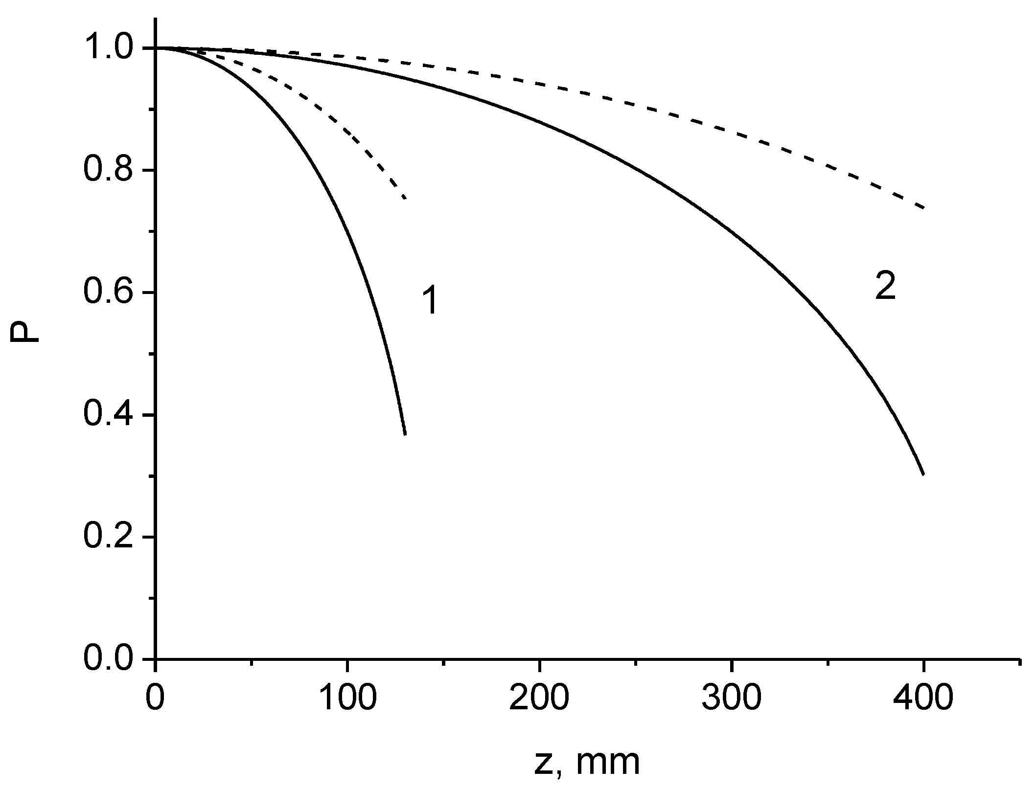
Figure 3.
The values as a function of the distance at x0 = 15 μm for both meridional and sagittal rays (solid curve 1) and only for meridional rays (dashed curve 2).
Figure 3.
The values as a function of the distance at x0 = 15 μm for both meridional and sagittal rays (solid curve 1) and only for meridional rays (dashed curve 2).
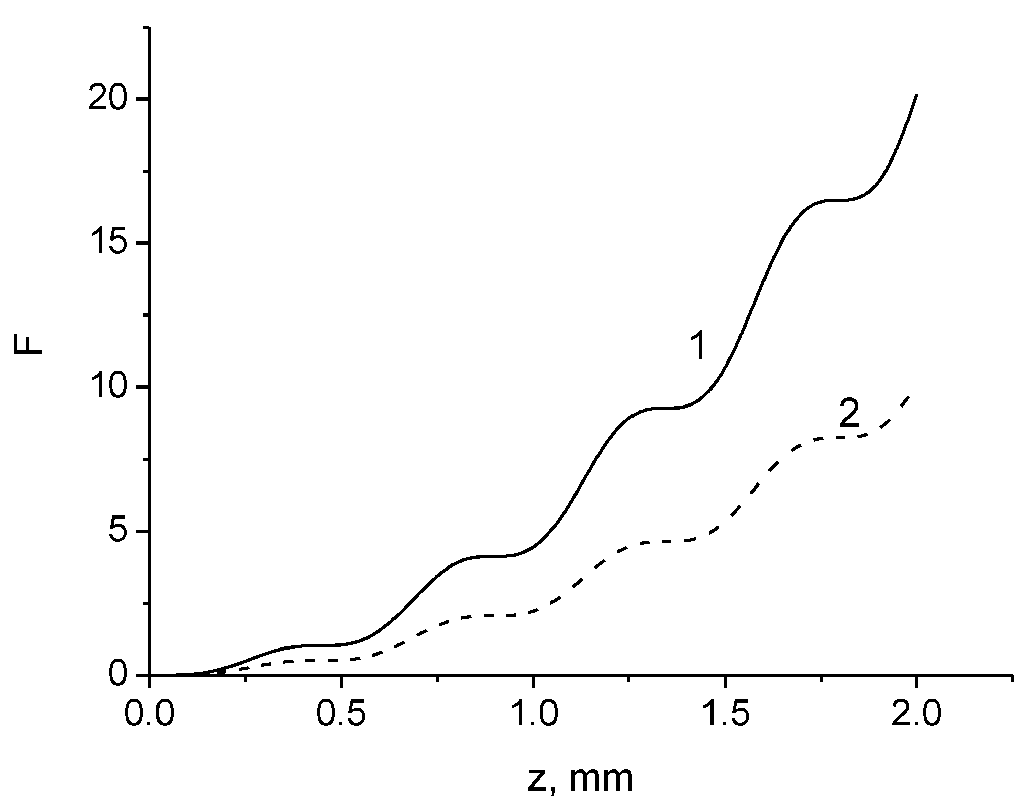
Figure 4.
The values as a function of distance for x0 = 15 μm; curve 1—sagittal ray with positive helicity (); curve 2—sagittal ray with negative helicity (); curve 3—meridional ray.
Figure 4.
The values as a function of distance for x0 = 15 μm; curve 1—sagittal ray with positive helicity (); curve 2—sagittal ray with negative helicity (); curve 3—meridional ray.

Figure 5.
The dependence of the angle of rotation of the polarization plane on (a) tilt angle of the beam relative to the fiber axis; (b) offset in a graded-index optical fiber with the parameters μm−1, n0 = 1.5, and the length z = 5 cm.
Figure 5.
The dependence of the angle of rotation of the polarization plane on (a) tilt angle of the beam relative to the fiber axis; (b) offset in a graded-index optical fiber with the parameters μm−1, n0 = 1.5, and the length z = 5 cm.

Figure 6.
Dependence of the rotation angle of the polarization plane on the tilt angle of the beam relative to the axis of an optical fiber of length 7.5 cm; theoretical (solid curve) and experimental [13] values (triangles).
Figure 6.
Dependence of the rotation angle of the polarization plane on the tilt angle of the beam relative to the axis of an optical fiber of length 7.5 cm; theoretical (solid curve) and experimental [13] values (triangles).

Figure 7.
Field amplitudes of even modes (a) and odd modes (b).

Figure 8.
Intensity distributions of the transverse electric field component (left column) and the longitudinal electric field component (right column) in the focal planes (a–d) and (e–h): (a,b) ; (c,d) —3D intensity patterns; (e,f) ; (g,h) .
Figure 8.
Intensity distributions of the transverse electric field component (left column) and the longitudinal electric field component (right column) in the focal planes (a–d) and (e–h): (a,b) ; (c,d) —3D intensity patterns; (e,f) ; (g,h) .

Figure 9.
Dependence of the delay time (a) and group delay splitting (b) on the radial and azimuthal indices, accordingly, z = 1 km, .
Figure 9.
Dependence of the delay time (a) and group delay splitting (b) on the radial and azimuthal indices, accordingly, z = 1 km, .
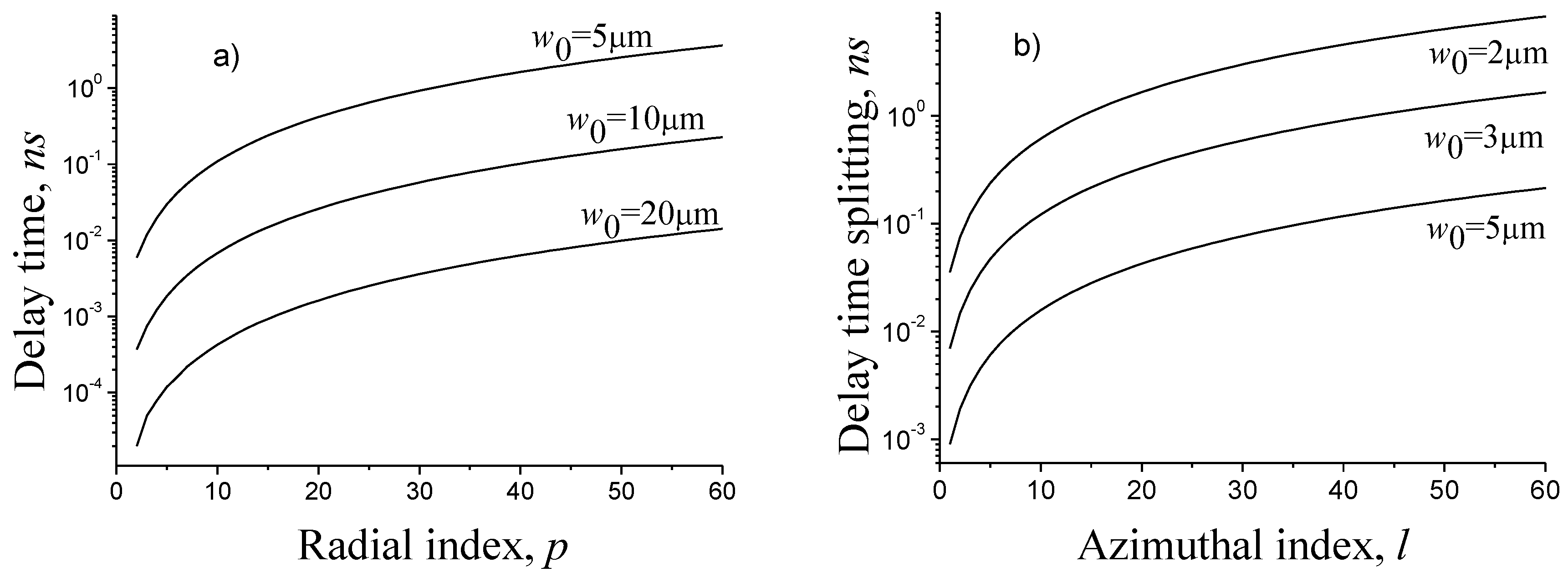
Figure 10.
Dependence of the mode splitting (a) and degeneracy lifting (b) on the azimuthal index. .
Figure 10.
Dependence of the mode splitting (a) and degeneracy lifting (b) on the azimuthal index. .

Figure 11.
Geometrical representation of possible vector polarization states. The vector polarization state is determined by the point P in the sphere and the degree of vector polarization by the length of vector OP: , Rv = OP. The maximum radius of the sphere is .
Figure 11.
Geometrical representation of possible vector polarization states. The vector polarization state is determined by the point P in the sphere and the degree of vector polarization by the length of vector OP: , Rv = OP. The maximum radius of the sphere is .

Figure 12.
Admissible values of combined vector and tensor polarization states are defined by the point P in a cone inserted into a sphere with the radius . The cross-section aAc of the cone is the equilateral triangle.
Figure 12.
Admissible values of combined vector and tensor polarization states are defined by the point P in a cone inserted into a sphere with the radius . The cross-section aAc of the cone is the equilateral triangle.

Publisher’s Note: MDPI stays neutral with regard to jurisdictional claims in published maps and institutional affiliations. |
© 2021 by the author. Licensee MDPI, Basel, Switzerland. This article is an open access article distributed under the terms and conditions of the Creative Commons Attribution (CC BY) license (https://creativecommons.org/licenses/by/4.0/).
Share and Cite
MDPI and ACS Style
Petrov, N.I. Depolarization of Light in Optical Fibers: Effects of Diffraction and Spin-Orbit Interaction. Fibers 2021, 9, 34. https://0-doi-org.brum.beds.ac.uk/10.3390/fib9060034
AMA Style
Petrov NI. Depolarization of Light in Optical Fibers: Effects of Diffraction and Spin-Orbit Interaction. Fibers. 2021; 9(6):34. https://0-doi-org.brum.beds.ac.uk/10.3390/fib9060034
Chicago/Turabian StylePetrov, Nikolai I. 2021. "Depolarization of Light in Optical Fibers: Effects of Diffraction and Spin-Orbit Interaction" Fibers 9, no. 6: 34. https://0-doi-org.brum.beds.ac.uk/10.3390/fib9060034
Note that from the first issue of 2016, this journal uses article numbers instead of page numbers. See further details here.