Coupled Projection Transfer Metric Learning for Cross-Session Emotion Recognition from EEG

Abstract

Distribution discrepancies between different sessions greatly degenerate the performance of video-evoked electroencephalogram (EEG) emotion recognition. There are discrepancies since the EEG signal is weak and non-stationary and these discrepancies are manifested in different trails in each session and even in some trails which belong to the same emotion. To this end, we propose a Coupled Projection Transfer Metric Learning (CPTML) model to jointly complete domain alignment and graph-based metric learning, which is a unified framework to simultaneously minimize cross-session and cross-trial divergences. By experimenting on the SEED_IV emotional dataset, we show that (1) CPTML exhibits a significantly better performance than several other approaches; (2) the cross-session distribution discrepancies are minimized and emotion metric graph across different trials are optimized in the CPTML-induced subspace, indicating the effectiveness of data alignment and metric exploration; and (3) critical EEG frequency bands and channels for emotion recognition are automatically identified from the learned projection matrices, providing more insights into the occurrence of the effect.

1. Introduction

Endowing machines with emotional intelligence is indispensable for natural human–machine interactions, making machines more humanized in communication [1,2]. EEG directly manifests electrical activities of the human cerebral cortex, providing an objective and reliable approach for emotion recognition [3]. Nowadays, EEG-based emotion recognition has received increasing attention from researchers due to its inherent characteristics, such as being noninvasive, inexpensive and easy to use. In view of these advantages, EEG-based emotion recognition has potential applications in diverse fields such as healthcare, education, entertainment and neuromarketing [4,5,6].

A typical EEG-based emotion recognition system is shown in Figure 1, which is usually composed of three stages. First, emotional video clips are played to healthy subjects to evoke their corresponding emotional states, while raw EEG data are recorded from them using EEG acquisition devices. Second, the raw EEG data will be preprocessed, including removing artifacts and down-sampling. Third, features will be extracted and then fed into a model to conduct emotion recognition. In this paper, we mainly focus on the third stage. In the past decade, lots of emotion recognition models ranging from machine learning to deep learning have been proposed [3,7]. For example, Shen et al. designed a multi-scale frequency bands ensemble learning model for EEG-based emotion classification, which effectively combined the information from different scales of frequency bands and further enhanced the performance [8]. Gao et al. proposed a coincidence-filtering-based approach to combine the advantages of both artificial-features-based methods and convolutional neural networks for EEG emotion recognition [9].

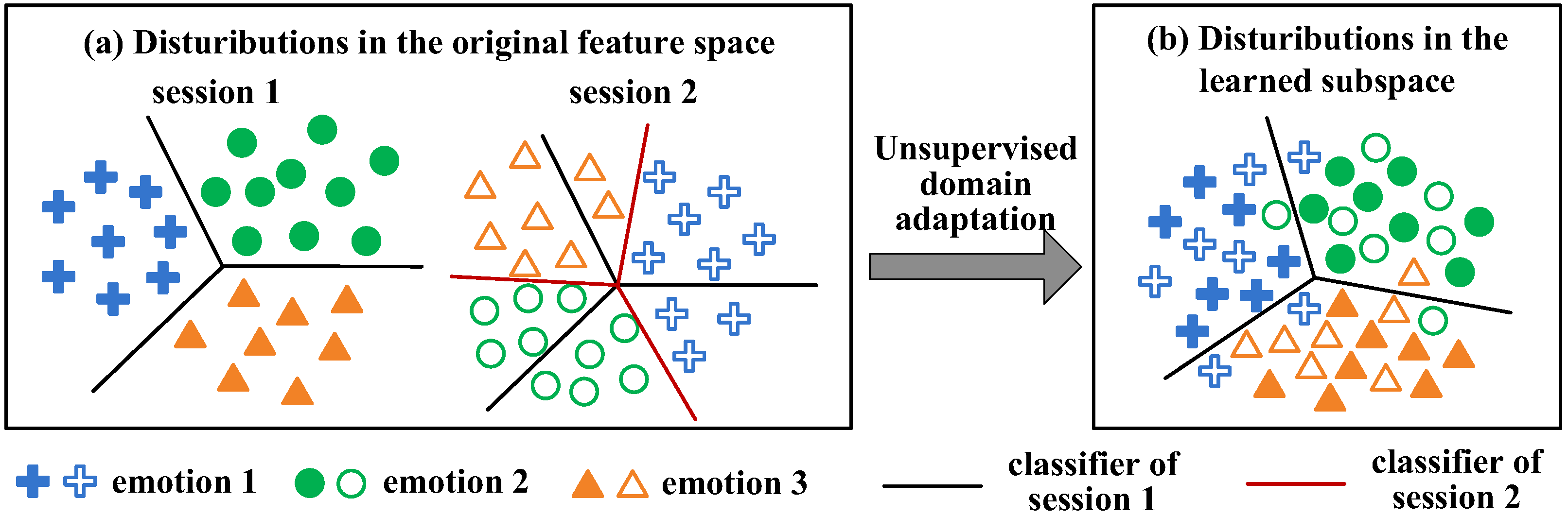
Nevertheless, the EEG signal is weak and non-stationary such that even for the same subject, distributions of EEG samples collected in different sessions cannot well match, which is generally known as cross-session discrepancies [10,11]. Figure 2a demonstrates a simple setting; that is, EEG samples of session 1 are collected on one day, and those of session 2 are collected on another day. Due to distribution discrepancies between these two sessions, even if a classifier is well trained by EEG samples from session 1, it may not achieve promising performance on session 2. To solve this problem, unsupervised domain adaptation (UDA) [12] has been introduced, which treats EEG samples of session 1 as the source domain and that of session 2 as the target domain, and then seeks a shared subspace of them to minimize distribution discrepancies, and thus improves the generalization ability of the source classifier, as shown in Figure 2b. According to UDA, Zheng et al. built several personalized EEG emotion recognition models by exploiting shared features and transferable model parameters between both domains [13]. Li et al. enforced the latent representations of the two domains to be similar and minimized the classification error of source domain [14]. These methods improved the cross-session emotion recognition performance in comparison with non-transfer methods.

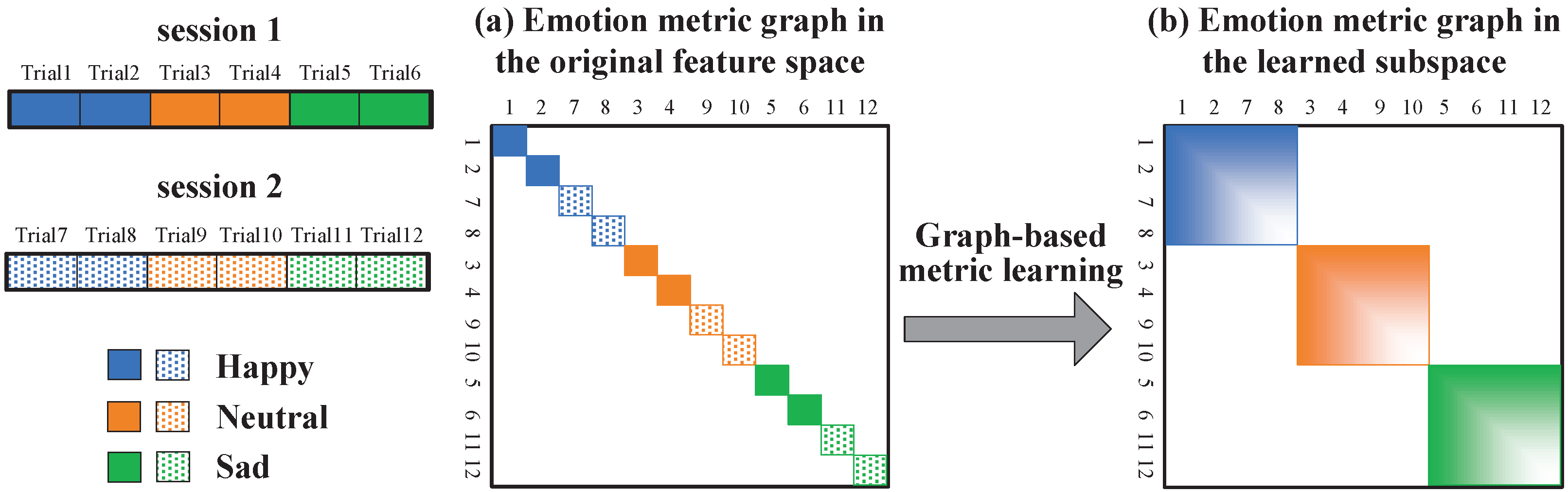
However, there are still some limitations in existing approaches. On the one hand, they only focus on the cross-session discrepancies of EEG, while ignoring the cross-trial differences. Generally, each session consists of multiple trials, each of which corresponds to a certain emotional state. Strictly, every trial is a slightly new task [10]. That is, there are differences among EEG samples from different trials but with the same emotional state, which is called as cross-trial differences. For example, supposing that there are six trials in each session with three emotional states, we build a similarity graph to depict the connectionship of these EEG samples [15], as shown in Figure 3a. Obviously, we obtain 12 rather than three diagonal blocks in the similarity graph, which is inconsistent with the ideal structure of a graph that the number of diagonal blocks should be equal to the number of emotional classes [16]. That is, the cross-trial differences of EEG are large and the similarity graph cannot well depict the underlying emotional states. Therefore, we should learn a more reliable emotion metric which can make EEG samples belonging to the same emotional state as interconnected as possible, whose corresponding similarity graph is shown in Figure 3b, such that the recognition performance can be greatly improved. On the other hand, most transfer methods mainly pursued higher emotion recognition accuracy and only a few of them may further explore what have been learned by the models. For example, Cui et al. developed a convolutional neural network combined with an interpretation technique for cross-subject driver drowsiness recognition [17]. They designed an interpretation technique to reveal relevant regions of the input signals that were important for prediction. However, their model required extra parameters to discovery common patterns of mental states across different subjects, which was time-consuming. Different from them, we directly explore the properties of the coupled projection matrices without extra parameters. The basis of it is that, from the perspective of transfer learning, the learned projection matrices mainly extract domain-invariant features by strengthening the common components between domains while weakening the non-common components. Therefore, they may reveal common information of the two different sessions which do not change over time. That is, we could conduct further investigations into them to explore the stable EEG patterns related to cross-session emotion expression.

To address both issues, we propose a model termed Coupled Projection Transfer Metric Learning (CPTML) for cross-session EEG emotion recognition, in order to not only improve the emotion recognition accuracy by minimizing both cross-session and cross-trial discrepancies of EEG data but also automatically reveal the stable EEG patterns of emotion from the learned subspace. Generally, CPTML projects data from two domains into respective subspaces by coupled projection matrices. Then, it unifies the domain alignment and the graph-based metric learning together into a single objective to jointly optimize the two subspaces. The main contributions of this paper are summarized below.

• We propose a transfer metric learning method to address two critical issues in cross-session EEG emotion recognition. Specifically, for the cross-session discrepancies, domain alignment is proposed to extract domain-invariant features, which makes distributions of the two sessions to be aligned; for the cross-trial differences, graph-based metric learning is designed to learn discriminative features, which makes EEG samples from different trials but belonging to the same emotional state to connect with each other. The extensive experimental results explicitly demonstrate the effectiveness of these two modules.
• We combine the domain alignment and the graph-based metric learning into a unified framework. On one hand, better aligned data can provide more accurate sample similarity measure for further graph-based metric learning; on the other hand, emotional discriminative features learned by metric learning can offer more accurate target pseudo labels, which further contributes to the conditional distribution alignment of both domains. Experimental results verify that these two modules are complementary to each other.
• Apart from improving emotion recognition accuracy, our CPTML model can explore the specific EEG patterns which are stable in cross-session emotion expression. It can automatically identify the critical EEG frequency bands and channels (brain regions) through investigating the feature weighting ability of the coupled projection matrices, which not only provides insights into the occurrence of affective effect, but also provides theory instruction for engineers to design wearable devices for emotion-related EEG acquisition.

The remaining contents are arranged as follows. In Section 2, we introduce the detailed formulation and optimization of our proposed CPTML model. The experiments were conducted to evaluate the efficacy of CPMTL in EEG emotion recognition in Section 3. Section 4 concludes the paper.

2. Methodology

2.1. Problem Definition

Suppose we have labeled EEG samples from one session $\{{\mathit{X}}_s,{\mathit{Y}}_s\}={\left\{({\mathit{x}}_{si},{\mathit{y}}_{si})\right\}}_{i=1}^{n_s}$, denoted as the source domain ${\mathcal{D}}_s$, and unlabeled EEG samples from the other session $\left\{{\mathit{X}}_t\right\}={\left\{{\mathit{x}}_{tj}\right\}}_{j=1}^{n_t}$, denoted as the target domain ${\mathcal{D}}_t$, where ${\mathit{X}}_s\in {\mathbb{R}}^{d\times n_s}$, ${\mathit{X}}_t\in {\mathbb{R}}^{d\times n_t}$, ${\mathit{Y}}_s\in {\mathbb{R}}^{C\times n_s}$, ${\mathit{x}}_{si},{\mathit{x}}_{tj}\in {\mathbb{R}}^d$, ${\mathit{y}}_{si}\in {\mathbb{R}}^C$ is a one-hot vector, d is the feature dimensionality, C is the number of emotional states, $n_s$ and $n_t$ are the number of samples in source and target domains, respectively. The feature space and label space of both domains are the same, i.e., ${\mathcal{X}}_s={\mathcal{X}}_t$ and ${\mathcal{Y}}_s={\mathcal{Y}}_t$; however, their marginal distributions and conditional distributions are different due to the domain shift: $P_s\left({\mathit{X}}_s\right)\ne P_t\left({\mathit{X}}_t\right)$ and $P_s\left({\mathit{Y}}_s\right|{\mathit{X}}_s)\ne P_t\left({\mathit{Y}}_t\right|{\mathit{X}}_t)$.

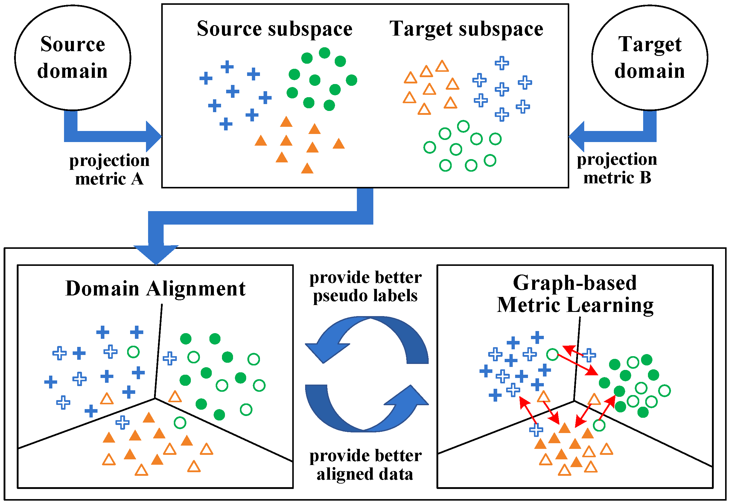
As shown in Figure 4, we project the source and target domain data into respective subspaces by two matrices, and then minimize the discrepancies between projected data of the two domains. Suppose $\mathit{A}\in {\mathbb{R}}^{d\times d_f}$ is the projection matrix for source domain, $\mathit{B}\in {\mathbb{R}}^{d\times d_f}$ is that for target domain, where $d_f$ ($d_f\ll d$) is the dimension of corresponding subspaces. Then, the projected data of the two domains can be represented as ${\mathit{A}}^T{\mathit{X}}_s$ and ${\mathit{B}}^T{\mathit{X}}_t$, respectively.

2.2. Domain Alignment

Due to the distribution discrepancies of EEG from different sessions, we simultaneously minimize marginal and conditional distributions between their projected representations according to the Maximum Mean Discrepancy (MMD) criterion [18]. In detail, marginal distribution alignment can be achieved by minimizing the distance between the sample means of the two domains; that is

$$F_{DistM}=\underset{\mathit{A},\mathit{B}}{min}\parallel \frac{1}{n_s}\sum _{i=1}^{n_s}{\mathit{A}}^T{\mathit{x}}_{si}-\frac{1}{n_t}\sum _{j=1}^{n_t}{\mathit{B}}^T{\mathit{x}}_{tj}{\parallel }^2.$$

(1)

Similarly, conditional distribution alignment aims to minimize the distance between the sample means belong to the same class of the two domains; that is

$$F_{DistC}=\underset{\mathit{A},\mathit{B}}{min}\sum _{c=1}^C\parallel \frac{1}{n_s^c}\sum _{i=1}^{n_s^c}{\mathit{A}}^T{\mathit{x}}_{si}-\frac{1}{n_t^c}\sum _{j=1}^{n_t^c}{\mathit{B}}^T{\mathit{x}}_{tj}{\parallel }^2,$$

(2)

where $n_s^c$ and $n_t^c$ denote the number of samples belonging to the ${c|}_{c=1}^C$-th emotional state in source and target domains, respectively. Since the label information of target domain data is not available, we utilize pseudo labels to estimate the conditional distribution in target domain, which is similar with [19,20]. Target pseudo labels are predicted by the classifier trained on source domain data and updated with iterations.

For simplicity, we combine $F_{DistM}$ and $F_{DistC}$ with the same weight. Thus, the joint distribution alignment is formulated as

$$F_{Dist}=F_{DistM}+F_{DistC}.$$

(3)

For clarity, we rewrite Equation (3) in matrix form as

$$\begin{array}{cc}\hfill F_{Dist}=& \underset{\mathit{A},\mathit{B}}{min}\mathrm{Tr}\left\{\begin{array}{cc}\hfill & {\mathit{A}}^T{\mathit{X}}_s{\mathit{U}}_{ss}{\mathit{X}}_s^T\mathit{A}\hfill \\ \hfill +& {\mathit{A}}^T{\mathit{X}}_s{\mathit{U}}_{st}{\mathit{X}}_t^T\mathit{B}\hfill \\ \hfill +& {\mathit{B}}^T{\mathit{X}}_t{\mathit{U}}_{ts}{\mathit{X}}_s^T\mathit{A}\hfill \\ \hfill +& {\mathit{B}}^T{\mathit{X}}_t{\mathit{U}}_{tt}{\mathit{X}}_t^T\mathit{B}\hfill \end{array}\right\},\hfill \end{array}$$

(4)

where

$$\begin{array}{c}{\mathit{U}}_{ss}={\mathit{P}}_{ss}+{\mathit{Q}}_{ss},{\mathit{U}}_{st}={\mathit{P}}_{st}+{\mathit{Q}}_{st},\\ \hfill {\mathit{U}}_{ts}={\mathit{P}}_{ts}+{\mathit{Q}}_{ts},{\mathit{U}}_{tt}={\mathit{P}}_{tt}+{\mathit{Q}}_{tt},\end{array}$$

(5)

$$\begin{array}{c}{\mathit{P}}_{ss}=\frac{1}{n_s^2}{\mathbf{1}}_s{\mathbf{1}}_s^T,{\mathit{P}}_{st}=\frac{-1}{n_s{n}_t}{\mathbf{1}}_s{\mathbf{1}}_t^T,\\ {\mathit{P}}_{ts}=\frac{-1}{n_t{n}_s}{\mathbf{1}}_t{\mathbf{1}}_s^T,{\mathit{P}}_{tt}=\frac{1}{n_t^2}{\mathbf{1}}_t{\mathbf{1}}_t^T,\end{array}$$

(6)

$$\begin{array}{c}{\mathit{Q}}_{ss}=\sum _{c=1}^C{\mathit{Q}}_{ss}^c,{\left({\mathit{Q}}_{ss}^c\right)}_{ij}=\left\{\begin{array}{cc}\frac{1}{{\left(n_s^c\right)}^2}\hfill & {\mathit{x}}_{si},{\mathit{x}}_{sj}\in {\mathit{X}}_s^c,\hfill \\ 0\hfill & \mathrm{otherwise},\hfill \end{array}\right.\end{array}$$

(7)

$$\begin{array}{c}{\mathit{Q}}_{st}=\sum _{c=1}^C{\mathit{Q}}_{st}^c,{\left({\mathit{Q}}_{st}^c\right)}_{ij}=\left\{\begin{array}{cc}\frac{-1}{n_s^c{n}_t^c}\hfill & {\mathit{x}}_{si}\in {\mathit{X}}_s^c,{\mathit{x}}_{tj}\in {\mathit{X}}_t^c,\hfill \\ 0\hfill & \mathrm{otherwise},\hfill \end{array}\right.\end{array}$$

(8)

$$\begin{array}{c}{\mathit{Q}}_{ts}=\sum _{c=1}^C{\mathit{Q}}_{ts}^c,{\left({\mathit{Q}}_{ts}^c\right)}_{ij}=\left\{\begin{array}{cc}\frac{-1}{n_t^c{n}_s^c}\hfill & {\mathit{x}}_{ti}\in {\mathit{X}}_t^c,{\mathit{x}}_{sj}\in {\mathit{X}}_s^c,\hfill \\ 0\hfill & \mathrm{otherwise},\hfill \end{array}\right.\end{array}$$

(9)

$$\begin{array}{c}{\mathit{Q}}_{tt}=\sum _{c=1}^C{\mathit{Q}}_{tt}^c,{\left({\mathit{Q}}_{tt}^c\right)}_{ij}=\left\{\begin{array}{cc}\frac{1}{{\left(n_t^c\right)}^2}\hfill & {\mathit{x}}_{ti},{\mathit{x}}_{tj}\in {\mathit{X}}_t^c\hfill \\ 0\hfill & \mathrm{otherwise},\hfill \end{array}\right.\end{array}$$

(10)

where ${\mathbf{1}}_s\in {\mathbb{R}}^{n_s}$ and ${\mathbf{1}}_t\in {\mathbb{R}}^{n_t}$ are all-one column vectors. Additionally, to avoid too much divergence between the two subspaces, we minimize the distance of them as

$$F_{Sub}=\underset{\mathit{A},\mathit{B}}{min}\mathrm{Tr}(\parallel \mathit{A}-\mathit{B}{\parallel }_F^2).$$

(11)

2.3. Graph-Based Metric Learning

Though discrepancies between source and target domains have been minimized, it still cannot guarantee that the projected data of the two domains can be discriminative enough for emotion recognition. As described in Section 1, discrepancies between different trials are large and EEG samples with the same emotional state cannot well connect with each other in the graph, leading to degenerated recognition performance. Therefore, we design a graph-based metric learning method to encourage the intra-class EEG sample pairs to stay close while the inter-class ones stay away. Specifically, for each domain, we leverage two kinds of graphs, i.e., intrinsic graph and penalty graph, to preserve the distance relationship between sample pairs [21,22]. In the intrinsic graph, each EEG sample is connected with $k_{intra}$ nearest samples within the same class in the same domain; while in the penalty graph, each EEG sample is connected with $k_{inter}$ nearest samples from different classes in the same domain. Then, we calculate the Laplacian matrix for each graph. Inspired by the Fisher criterion [23], it is intuitive to compact samples in the same class and separate samples in different classes, which can be achieved by

$$\begin{array}{c}\frac{F_{SrcI}}{F_{SrcP}}=\underset{\mathit{A},\mathit{B}}{min}\frac{\mathrm{Tr}\left({\mathit{A}}^T{\mathit{X}}_s{\mathit{L}}_I^s{\mathit{X}}_s^T\mathit{A}\right)}{\mathrm{Tr}\left({\mathit{A}}^T{\mathit{X}}_s{\mathit{L}}_P^s{\mathit{X}}_s^T\mathit{A}\right)},\end{array}$$

(12)

$$\begin{array}{c}\frac{F_{TgtI}}{F_{TgtP}}=\underset{\mathit{A},\mathit{B}}{min}\frac{\mathrm{Tr}\left({\mathit{B}}^T{\mathit{X}}_t{\mathit{L}}_I^t{\mathit{X}}_t^T\mathit{B}\right)}{\mathrm{Tr}\left({\mathit{B}}^T{\mathit{X}}_t{\mathit{L}}_P^t{\mathit{X}}_t^T\mathit{B}\right)},\end{array}$$

(13)

where ${\mathit{L}}_I^s\in {\mathbb{R}}^{n_s\times n_s}$ and ${\mathit{L}}_P^s\in {\mathbb{R}}^{n_s\times n_s}$ represent the Laplacian matrix of the intrinsic and penalty graphs in the source domain, respectively; ${\mathit{L}}_I^t\in {\mathbb{R}}^{n_t\times n_t}$ and ${\mathit{L}}_P^t\in {\mathbb{R}}^{n_t\times n_t}$ are those in the target domain. The Laplacian matrix is calculated as $\mathit{L}=\mathit{D}-({\mathit{S}}^T+\mathit{S})/2$, where $\mathit{S}$ is the weight matrix, and ${\mathit{D}}_{ii}={\sum }_j{\mathit{S}}_{ij}$. In this paper, the weight matrix $\mathit{S}$ is computed by the “HeatKernel” function, i.e., ${\mathit{S}}_{ij}$ would be $\exp (-(\parallel {\mathit{x}}_i-{\mathit{x}}_j{\parallel }^2)/2)$ if ${\mathit{x}}_i$ and ${\mathit{x}}_j$ are connected, otherwise it would be 0.

2.4. Overall Objective Function

As stated previously, domain alignment and graph-based metric learning are complementary to each other. On one hand, domain alignment offers better aligned data based on which more accurate sample-pair distance and class information can be obtained for subsequent graph-based metric learning; on the other hand, emotional discriminative features learned by graph-based metric learning can help to predict more accurate target labels, which is beneficial for better aligning the conditional distributions. Therefore, we joint them into a unified framework.

Further, we impose two constraints on the target subspace as [24,25] did. First, to avoid features of the target domain data being projected into irrelevant dimensions, we maximize the variance of the target projected data by $F_{Cons1}={max}_{\mathit{B}}\mathrm{Tr}\left({\mathit{B}}^T{\mathit{X}}_t{\mathit{O}}_t{\mathit{X}}_t^T\mathit{B}\right)$, where ${\mathit{O}}_t={\mathit{I}}_t-\frac{1}{n_t}{\mathbf{1}}_t{\mathbf{1}}_t^T$ is the centering matrix, ${\mathit{I}}_t\in {\mathbb{R}}^{n_t\times n_t}$ is the identity matrix. Second, we control the scale of target subspace by $F_{Cons2}={min}_{\mathit{B}}\mathrm{Tr}\left({\mathit{B}}^T\mathit{B}\right)$. Thus, the final objective function of CPTML can be formulated as

$$F=min\frac{F_{Dist}+\lambda F_{Sub}+\gamma (F_{SrcI}+F_{TgtI})+\mu F_{Cons2}}{\gamma (F_{SrcP}+F_{TgtP})+\mu F_{Cons1}},$$

(14)

where $\lambda$, $\gamma$ and $\mu$ are trade-off parameters. It can be rewritten it into the following form

$$F=\underset{\mathit{A},\mathit{B}}{min}\frac{\mathrm{Tr}\left\{\begin{array}{cc}\hfill & {\mathit{A}}^T({\mathit{X}}_s({\mathit{U}}_{ss}+\gamma {\mathit{L}}_I^s){\mathit{X}}_s^T+\lambda \mathit{I})\mathit{A}\hfill \\ \hfill +& {\mathit{A}}^T({\mathit{X}}_s{\mathit{U}}_{st}{\mathit{X}}_t^T-\lambda \mathit{I})\mathit{B}\hfill \\ \hfill +& {\mathit{B}}^T({\mathit{X}}_t{\mathit{U}}_{ts}{\mathit{X}}_s^T-\lambda \mathit{I})\mathit{A}\hfill \\ \hfill +& {\mathit{B}}^T({\mathit{X}}_t({\mathit{U}}_{tt}+\gamma {\mathit{L}}_I^t){\mathit{X}}_t^T+(\lambda +\mu )\mathit{I})\mathit{B}\hfill \end{array}\right\}}{\mathrm{Tr}\left\{\begin{array}{cc}\hfill & {\mathit{A}}^T{\mathit{X}}_s\left(\gamma {\mathit{L}}_P^s\right){\mathit{X}}_s^T\mathit{A}\hfill \\ \hfill +& {\mathit{B}}^T{\mathit{X}}_t(\gamma {\mathit{L}}_P^t+\mu {\mathit{O}}_t){\mathit{X}}_t^T\mathit{B}\hfill \end{array}\right\}},$$

(15)

where $\mathit{I}\in {\mathbb{R}}^{d\times d}$ is the identity matrix. To enhance the readability, we transform Equation (15) into the matrix form as

$$F=\underset{\mathit{A},\mathit{B}}{min}\frac{\mathrm{Tr}(\left[\begin{array}{cc}{\mathit{A}}^T& {\mathit{B}}^T\end{array}\right]\left[\begin{array}{cc}{\mathit{W}}_{ss}& {\mathit{W}}_{st}\\ {\mathit{W}}_{ts}& {\mathit{W}}_{tt}\end{array}\right]\left[\begin{array}{c}\mathit{A}\\ \mathit{B}\end{array}\right])}{\mathrm{Tr}(\left[\begin{array}{cc}{\mathit{A}}^T& {\mathit{B}}^T\end{array}\right]\left[\begin{array}{cc}{\mathit{R}}_{ss}& \mathbf{0}\\ \mathbf{0}& {\mathit{R}}_{tt}\end{array}\right]\left[\begin{array}{c}\mathit{A}\\ \mathit{B}\end{array}\right])},$$

(16)

where $\mathbf{0}\in {\mathbb{R}}^{d\times d}$, and

$$\left\{\begin{array}{cc}\hfill {\mathit{W}}_{ss}& ={\mathit{X}}_s({\mathit{U}}_{ss}+\gamma {\mathit{L}}_I^s){\mathit{X}}_s^T+\lambda \mathit{I}\hfill \\ \hfill {\mathit{W}}_{st}& ={\mathit{X}}_s{\mathit{U}}_{st}{\mathit{X}}_t^T-\lambda \mathit{I}\hfill \\ \hfill {\mathit{W}}_{ts}& ={\mathit{X}}_t{\mathit{U}}_{ts}{\mathit{X}}_s^T-\lambda \mathit{I}\hfill \\ \hfill {\mathit{W}}_{tt}& ={\mathit{X}}_t({\mathit{U}}_{tt}+\gamma {\mathit{L}}_I^t){\mathit{X}}_t^T+(\lambda +\mu )\mathit{I}\hfill \end{array}\right.,$$

(17)

$$\left\{\begin{array}{cc}\hfill {\mathit{R}}_{ss}& ={\mathit{X}}_s\left(\gamma {\mathit{L}}_P^s\right){\mathit{X}}_s^T\hfill \\ \hfill {\mathit{R}}_{tt}& ={\mathit{X}}_t(\gamma {\mathit{L}}_P^t+\mu {\mathit{O}}_t){\mathit{X}}_t^T\hfill \end{array}\right..$$

(18)

2.5. Optimization

The two projection matrices $\mathit{A}$ and $\mathit{B}$ are the target variables to be optimized in Equation (16), which is obviously a generalized Rayleigh quotient and can be optimized by generalized eigenvalue decomposition. By denoting $\mathit{H}\triangleq [\mathit{A};\mathit{B}]$, we introduce an Lagrange multiplier $\mathsf{\Phi }$ and the Lagrangian function of Equation (16) can be transformed as

$$\left[\begin{array}{cc}{\mathit{R}}_{ss}& \mathbf{0}\\ \mathbf{0}& {\mathit{R}}_{tt}\end{array}\right]\mathit{H}=\left[\begin{array}{cc}{\mathit{W}}_{ss}& {\mathit{W}}_{st}\\ {\mathit{W}}_{ts}& {\mathit{W}}_{tt}\end{array}\right]\mathit{H}\mathsf{\Phi },$$

(19)

where $\mathsf{\Phi }=diag({\varphi }_1,\cdots ,{\varphi }_{d_f})$ and ${\varphi }_1,\cdots ,{\varphi }_{d_f}$ are the $d_f$ largest eigenvalues of the above eigendecomposition problem, and $\mathit{H}=[{\mathit{H}}_1,\cdots ,{\mathit{H}}_{d_f}]$ contains the corresponding $d_f$ eigenvectors. Once the matrix $\mathit{H}$ is solved, the optimal projection matrices $\mathit{A}$ and $\mathit{B}$ can be obtained. The procedures of the proposed method CPTML is shown in Algorithm 1.

2.6. Computational Complexity

The computational complexity of CPTML consists of the following two parts. First, computing ${\mathit{W}}_{ss}$, ${\mathit{W}}_{st}$, ${\mathit{W}}_{ts}$, ${\mathit{W}}_{tt}$, ${\mathit{R}}_{ss}$ and ${\mathit{R}}_{tt}$ in step 3 of Algorithm 1 costs $O\left(TC{n}^2\right)$, where $n=n_s+n_t$. Second, solving the generalized eigenvalue decomposition problem in step 4 of Algorithm 1 costs $O\left(Td{d}_f^2\right)$. Finally, the computational complexity of CPTML is $O(TC{n}^2+Td{d}_f^2)$. Specifically, in this paper, T is less than 30, which is enough to ensure convergence of the algorithm, and $d_f\ll d\ll n$.

Algorithm 1 The procedure for CPTML framework.

Input:  Data and labels of the source domain $\{{\mathit{X}}_s,{\mathit{Y}}_s\}$, data of the target domain ${\mathit{X}}_t$; Parameters $d_f$, $k_{intra}$, $k_{inter}$, $\lambda$, $\gamma$ and $\mu$; Output:  Projection matrices $\mathit{A}$ and $\mathit{B}$, classifier f, and labels of the target domain data $\widehat{{\mathit{Y}}_t}$. 1: Initialize $\mathit{A}=\mathit{B}$ with Principal Component Analysis (PCA), and train a classifier f by ${\ell }_2$-norm Regularized Least Square Regression (${\ell }_2$-LSR) on the source projected data $\{{\mathit{A}}^T{\mathit{X}}_s,{\mathit{Y}}_s\}$; then predict the pseudo labels of the target domain data with the trained classifier $\widehat{{\mathit{Y}}_t}=f\left({\mathit{B}}^T{\mathit{X}}_t\right)$; 2: while not converge do 3:    Compute $\left[\begin{array}{cc}{\mathit{W}}_{ss}& {\mathit{W}}_{st}\\ {\mathit{W}}_{ts}& {\mathit{W}}_{tt}\end{array}\right]$ and $\left[\begin{array}{cc}{\mathit{R}}_{ss}& \mathbf{0}\\ \mathbf{0}& {\mathit{R}}_{tt}\end{array}\right]$ by Equations (17) and (18), respectively; 4:    Solve the generalized eigenvalue decomposition problem in Equation (19), and obtain matrix $\mathit{H}$ by choosing $d_f$ eigenvectors corresponding to $d_f$ largest eigenvalues, then $\mathit{A}$ and $\mathit{B}$ can update according to $\mathit{H}=[\mathit{A};\mathit{B}]$; 5:    Train a new classifier f by ${\ell }_2$-LSR on the updated source projection data $\{{\mathit{A}}^T{\mathit{X}}_s,{\mathit{Y}}_s\}$; then update the pseudo labels of the target domain data $\widehat{{\mathit{Y}}_t}=f\left({\mathit{B}}^T{\mathit{X}}_t\right)$; 6: end while

3. Experiments

3.1. Dataset

SEED_IV [11] is a widely used dataset for EEG-based emotion recognition. It is a video-evoked EEG dataset, and 72 carefully chosen video clips are used to elicit four desired emotion states (sad, fear, happy, and neutral). A total of 15 healthy subjects participated in the EEG data collection experiment 3 times on different days, corresponding to 3 sessions. In each session, each subject was asked to watch 24 video clips (6 video clips corresponding to one emotional state) to evoke the four emotional states. That is, each session has 24 trials. During watching video clips, EEG data of subjects were recorded by the ESI NeuroScan system with a 62-channel cap whose electrodes are placed according to the standard 10–20 system.

Differential entropy (DE) feature of EEG data is used to evaluate performance of models in our experiment, which is the preprocessed version of the SEED_IV dataset and can be downloaded from https://bcmi.sjtu.edu.cn/home/seed/seed-iv.html (accessed on 25 March 2022). The DE feature also has been proved that it is the most stable and accurate feature for emotion recognition than traditional features [26,27]. Since the DE features were extracted from 5 different EEG frequency bands, including Delta (1–4 Hz), Theta (4–8 Hz), Alpha (8–14 Hz), Beta (14–31 Hz), Gamma (31–50 Hz), and there are 62 channels in total, the data format is $62\times n\times 5$. n is the number of samples for each subject in each session, which is approximate 830. We reshape DE features into $310\times n$ by concatenating the 62 values of 5 frequency bands into a vector and then normalize them into [−1, 1] by row and conduct decentralizing.

3.2. Experimental Settings

To investigate the performance of CPTML in the cross-session EEG emotion recognition task, we set experiments as follows. For every subject, samples as well as their labels from one session form the labeled source domain and samples from the other session form the target domain. Therefore, each subject has three cross-session tasks in chronological order, i.e., “session 1 → session 2”, “session 1 → session 3” and “session 2 → session 3”, respectively.

We compare CPTML with several other models including the joint distribution adaptation (JDA) [19], subspace distribution alignment (SDA) [28], jointly optimized semi-supervised RVFL (JOSRVFL) [29] and joint domain adaptation and semi-supervised RVFL network (JDASRN) [30]. For JDA, SDA and CPTML, the dimensionality of feature subspace $d_f$ is determined by grid search from $\{5,10,\cdots ,40\}$. For JDA and CPTML, the maximal number of iterations T is set as 30. In CPTML, $k_{intra}$ and $k_{inter}$ are searched from $\{5,10,\cdots ,60\}$. $\lambda$, $\gamma$ and $\mu$ are searched from $5\times \{{10}^{-2},{10}^{-1},\cdots ,{10}^2\}$. The classifier used in this paper is ${\ell }_2$-LSR and the regularization parameter is searched from $\{{10}^{-5},{10}^{-4},\cdots ,{10}^5\}$. Additionally, since the experimental settings of JOSRVFL and JDASRN are identical to ours, we directly use their published results.

3.3. Recognition Results and Analysis

The results of the five models on the three cross-session EEG emotion recognition tasks are, respectively, shown in

Table 1. Recognition accuracies (%) on the session 1 → session 2 task.

Subjects	JDA	SDA	JOSRVFL	JDASRN	CPTML
ID1	63.22	70.79	71.51	76.44	88.70
ID2	92.55	91.23	87.38	96.63	97.36
ID3	68.99	69.59	70.55	69.59	91.23
ID4	64.30	81.37	80.17	68.87	85.94
ID5	71.15	59.98	80.17	68.15	88.58
ID6	64.98	63.22	67.43	79.09	66.95
ID7	73.08	85.10	91.23	87.86	94.35
ID8	74.04	76.20	83.89	81.61	83.97
ID9	72.64	59.01	78.25	84.01	73.80
ID10	64.18	53.25	59.13	71.75	75.24
ID11	62.98	63.58	56.49	68.15	64.54
ID12	55.41	60.94	61.90	56.13	66.11
ID13	64.42	61.21	67.55	71.75	72.84
ID14	67.79	77.76	82.33	82.33	84.01
ID15	93.03	95.67	93.15	98.80	98.80
Average	70.18	71.26	75.41	77.41	82.16

,

Table 2. Recognition accuracies (%) on the session 1 → session 3 task.

Subjects	JDA	SDA	JOSRVFL	JDASRN	CPTML
ID1	62.53	77.01	80.90	73.11	84.67
ID2	65.33	58.52	83.33	87.23	88.69
ID3	53.28	42.09	56.45	70.80	74.21
ID4	77.74	86.25	85.04	89.90	93.07
ID5	70.19	72.51	84.55	74.94	85.40
ID6	80.90	75.79	76.64	86.37	84.79
ID7	56.57	85.16	85.64	81.27	90.15
ID8	81.75	89.42	81.14	92.09	94.89
ID9	58.27	52.43	62.29	70.92	80.54
ID10	64.84	70.21	61.07	73.48	73.51
ID11	66.06	67.82	74.33	81.75	85.89
ID12	54.26	51.70	67.15	52.07	74.45
ID13	56.84	40.88	47.81	70.44	63.02
ID14	83.82	81.39	84.79	89.54	89.54
ID15	80.54	78.22	82.60	92.58	92.58
Average	67.53	68.63	74.25	79.10	83.69

and

Table 3. Recognition accuracies (%) on the session 2 → session 3 task.

Subjects	JDA	SDA	JOSRVFL	JDASRN	CPTML
ID1	58.88	66.30	62.04	60.58	76.16
ID2	59.61	64.72	89.54	72.75	74.21
ID3	84.55	66.67	79.81	89.42	86.98
ID4	67.40	85.04	92.46	96.11	97.93
ID5	72.63	71.29	80.54	82.36	83.82
ID6	55.96	86.42	88.81	79.44	89.42
ID7	90.15	91.73	87.59	90.15	94.89
ID8	65.69	83.82	83.70	81.27	88.93
ID9	66.79	51.46	68.73	75.18	72.51
ID10	85.40	82.48	73.24	73.97	89.42
ID11	59.37	62.04	54.74	64.84	66.91
ID12	51.82	78.47	82.12	64.48	82.41
ID13	66.91	67.72	63.38	74.82	75.91
ID14	79.68	87.71	91.36	90.51	95.26
ID15	90.39	90.39	87.71	95.01	95.38
Average	70.35	75.75	79.05	79.39	84.68

, where we highlight the best accuracies in boldface. From the obtained results, we made the following observations: (1) Generally, CPTML performs the best among these five models. It obtains the highest recognition accuracies in most of the total 45 cases and the best average accuracies of 82.16%, 83.69% and 84.68% in all the three cross-session EEG emotion recognition tasks, indicating the superiority of joint data alignment and emotion metric learning. (2) The strategy of simultaneously minimizing cross-session and cross-trial discrepancies performs better than considering only one of them. Specifically, as shown in Table 1, CPTML achieves 11.98% and 10.90% improvements in comparison with JDA and SDA which only take into account the discrepancies between different sessions. Similar phenomena can also be found in Table 2 and Table 3. Additionally, compared with JOSRVFL which mainly focuses on learning discriminative features from EEG samples, CPTML exceeds it by 6.75%, 9.44% and 5.62% in the three cross-session tasks, respectively. (3) CPTML outperforms JDASRN by 4.75%, 4.59% and 5.28% in the three tasks. The main difference between them is that CPTML employs a joint framework to complete the domain alignment and graph-based metric learning while JDASRN uses a two-stage manner. Since there inevitably exist interactions between these two modules, our CPTML model is more powerful in approximating the global optimum.

In addition to comparing the average accuracy rates of the five models, the Friedman test [31] is used to illustrate the statistical significance among them. It ranks all methods by combining the results on each group, and the higher ranking indicates the better performance of the corresponding model. The detail of the statistical test is stated as follows. The underlying hypothesis is that “all the models have the same performance”. Whether to accept the hypothesis or not is determined by the variable ${\tau }_F$, which is defined as

$${\tau }_F=\frac{(N-1){\tau }_{{\chi }^2}}{N(K-1)-{\tau }_{{\chi }^2}},$$

(20)

where K is the number of models, N is the number of result groups, and ${\tau }_{{\chi }^2}$ is calculated as

$${\tau }_{{\chi }^2}=\frac{12N}{K(K+1)}(\sum _{i=1}^K{r}_i^2-\frac{K{(K+1)}^2}{4}),$$

(21)

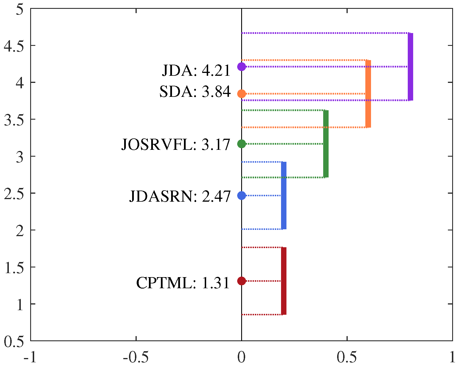
where $r_i$ is the average ranking of the i-th model. In this paper, $K=5$, $N=45$, the average rankings of the five models are $[4.21,3.84,3.17,2.47,1.31]$. We can obtain ${\tau }_F=50.51$ according to Equation (20). When the significance level $\alpha =0.05$ by default, the critical value of Friedman test is 2.423 [32]. It is obvious that ${\tau }_F=50.51$ is greater than 2.423; thus, the hypothesis is rejected. Further, the Nemenyi test is used to distinguish whether there are significant differences among these models, and the result is shown in Figure 5. In the figure, the solid circles denote the average rankings of these models, and the length of vertical line denotes the critical distance (CD) of Nemenyi test, which is calculated as

$$CD=q_{\alpha }\sqrt{\frac{K(K+1)}{6N}},$$

(22)

where $q_{\alpha }$ is the critical value and it is 2.728 when $\alpha =0.05$ [33]. If two vertical lines do not have overlap, it indicates that the corresponding models have statistically different performance. As shown in Figure 5, our proposed CPTML does not have overlap with JDASRN, JOSRVFL, SDA and JDA, which means that it is significantly better than the other four models in the cross-session emotion recognition tasks.

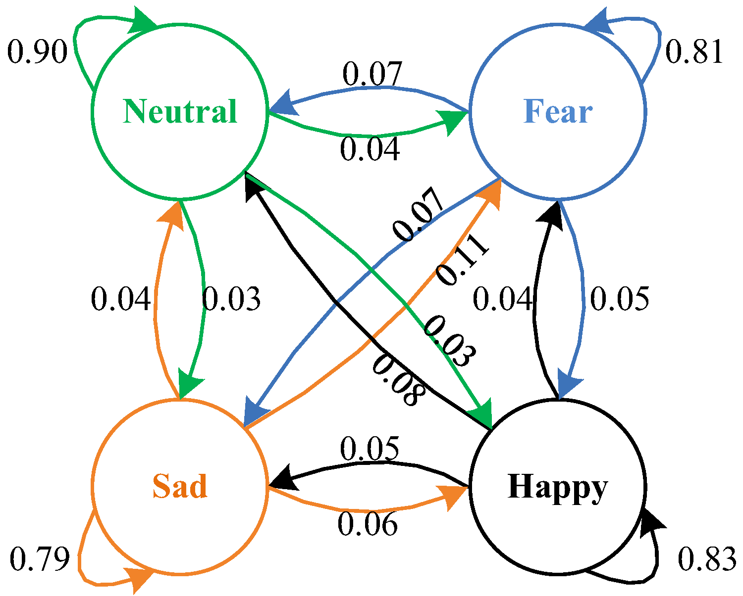
To give an insight into the recognition performance of CPTML on each emotional state, we use the average confusion graph to present the recognition results of the three cross-session tasks again in Figure 6. First, we obtain the average recognition accuracies of the four emotional states. For example, the average accuracies of the neutral, sad, fear and happy emotional states classified by CPTML are 90%, 79%, 81% and 83%, respectively. Second, the misclassification rates of all emotional states are explicitly provided. For example, 90% of the neutral EEG samples are correctly classified while 3%, 4% and 3% of them are wrongly recognized as sad, fear and happy states, respectively. Third, the neutral emotional state achieves the highest average accuracy in comparison with the others, which is the easiest one to recognize based on our experimental results.

3.4. Effect of Domain Alignment and Emotion Metric Learning

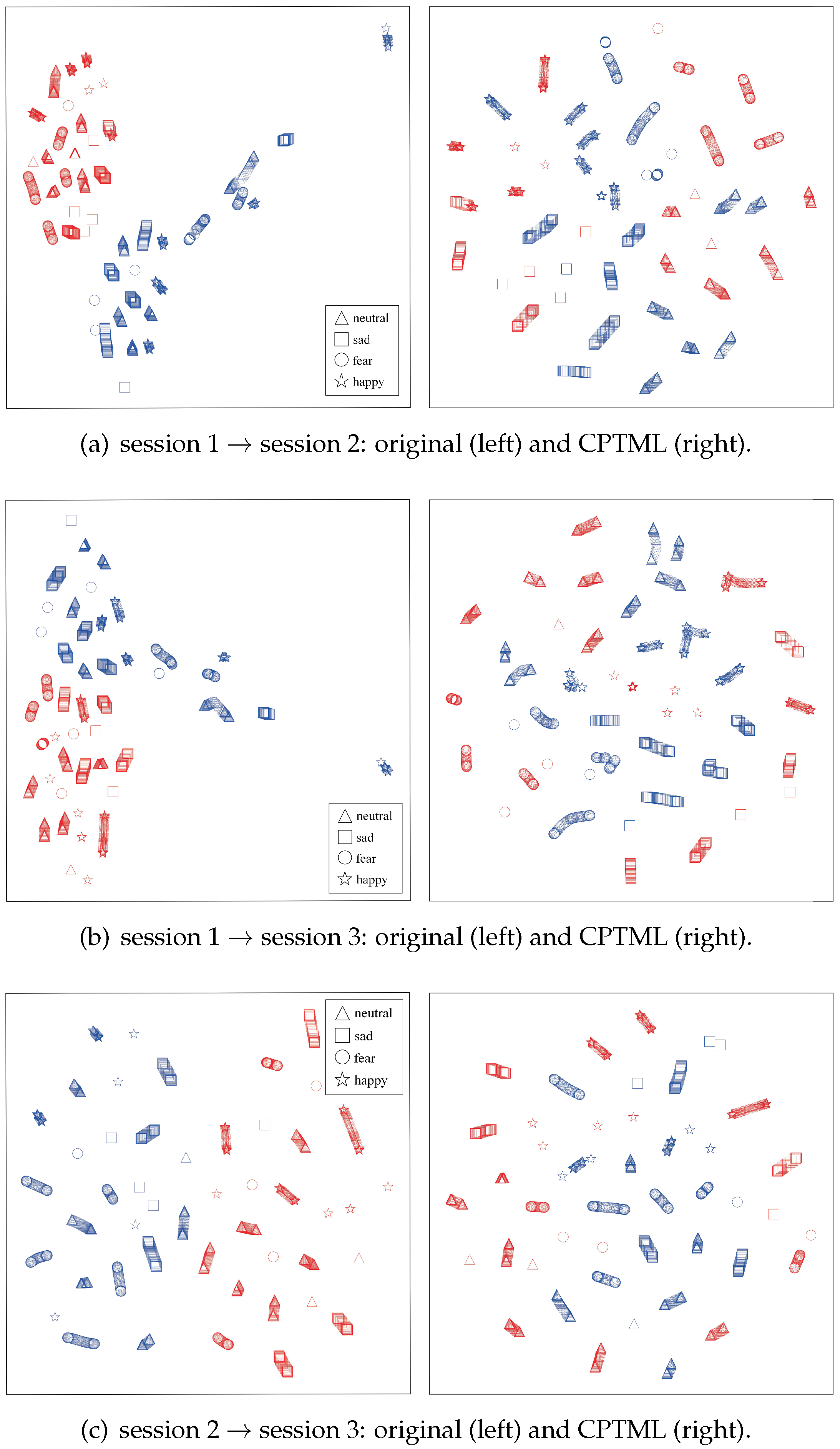
In this section, we first investigate the data alignment ability of CPTML in minimizing the domain discrepancies. As shown in Figure 7, by taking subject 5 as an example and using the t-SNE [34] visualization method, we intuitively plot the distributions of original data representation and CPTML-based subspace representation. From this figure, we find that the data distributions of the two domains are significantly different in original feature space; however, the discrepancies are dramatically reduced in the new subspaces learned by CPTML. This is exactly what the transfer learning does. In the learned subspaces, the source and target data share similar representations, benefiting from the joint marginal and conditional distributions alignment. This indicates that the domain alignment module of CPTML is effective for mitigating cross-session differences.

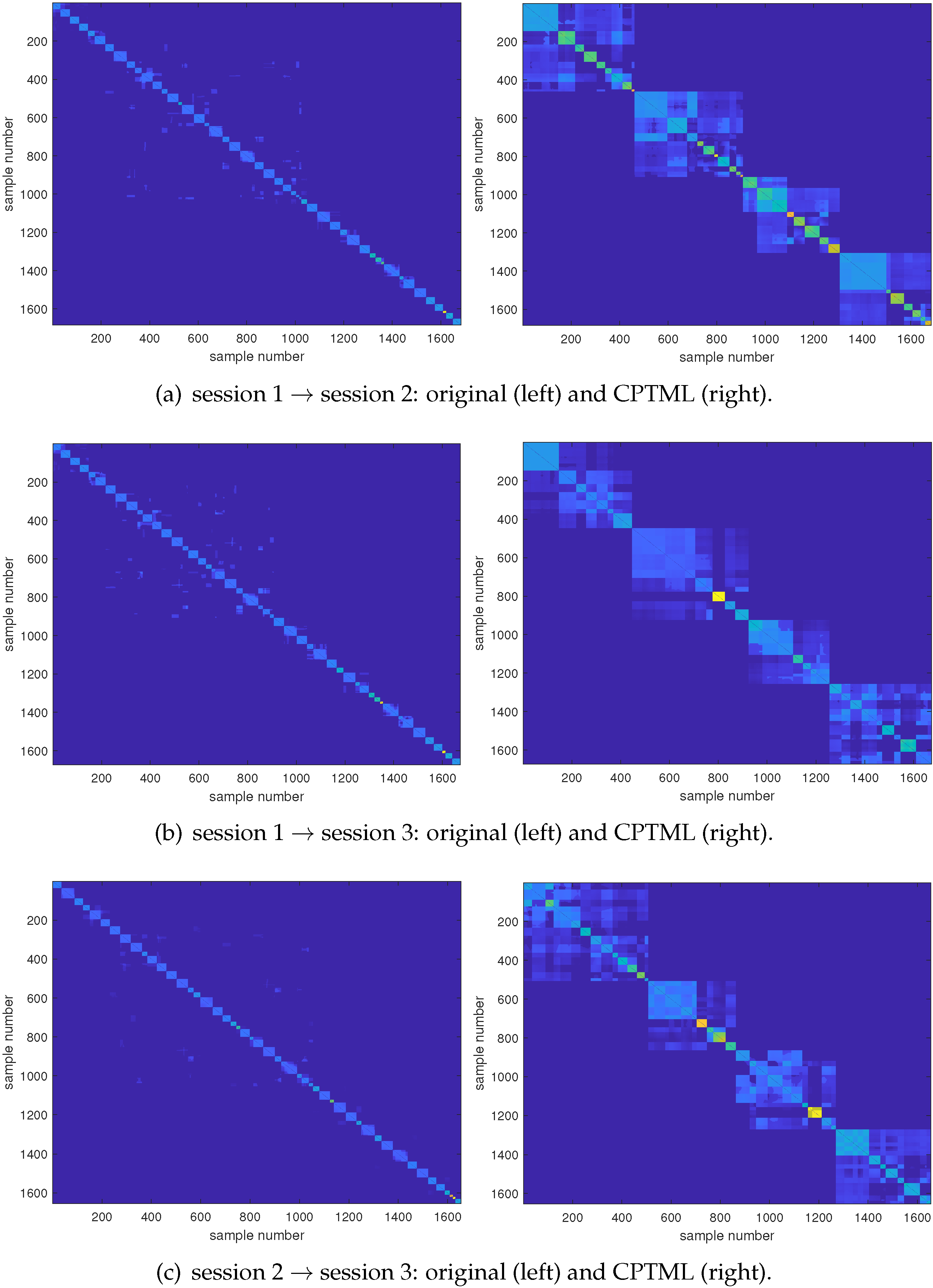
Second, we illustrate the effectiveness of CPTML in graph-based metric learning. By means of the similarity matrix which characterizes the connection among all source and target EEG samples, we can display the emotion metric graphs corresponding to original feature space and the learned CPTML subspaces. Figure 8 which also takes subject 5 as an example shows the learned results of its three cross-session recognition tasks. We observe that there are 48 block diagonals in the graphs of original feature space, which is exactly the total number of trials in source and target domains. According to the graph theory, since the value within each block denotes the affinity of two corresponding samples in one class, the number of block diagonals should be theoretically equal to the number of classes (i.e., 4 in present research since there are four emotional states in SEED_IV). The fact that the number of block diagonals in the left column of Figure 8 is 48 instead of 4 means that the cross-trial divergences are greater than those of different emotional states. Specifically, even two trials have the same emotional state, the similarities of samples in these two trials cannot be well built due to the large cross-trial differences. Fortunately, in the learned CPTML subspaces shown in the right column of Figure 8, the contours of the 4 block diagonals are significantly enhanced. It means that CPTML finds a way in appropriately building connections for EEG samples belonging to the same emotional state. We informally state this process as emotion metric learning, which corresponds to minimizing distances between intra-class samples and maximizing distances between inter-class samples.

3.5. Knowledge Discovery on Frequency Bands and Channels

For cross-session EEG emotion recognition, we are interested not only in the classification accuracy but also in the stable EEG patterns in cross-session emotion expression. Since the latter can offer us more insights to the neural mechanism of emotion processing, we expect the CPTML model to be competent for exploring where the cross-session stable EEG features are mainly from, i.e., identifying the critical EEG frequency bands and channels. From the perspective of transfer learning, it tries to seek shared subspaces for both source and target samples; therefore, the two coupled projection matrices $\mathit{A}$ and $\mathit{B}$ should learn domain-invariant features by strengthening the common components between domains while weakening the non-common components. Equivalently, we propose a quantitative approach to measure the feature weighting ability of the two projection matrices. Below are the detailed procedures.

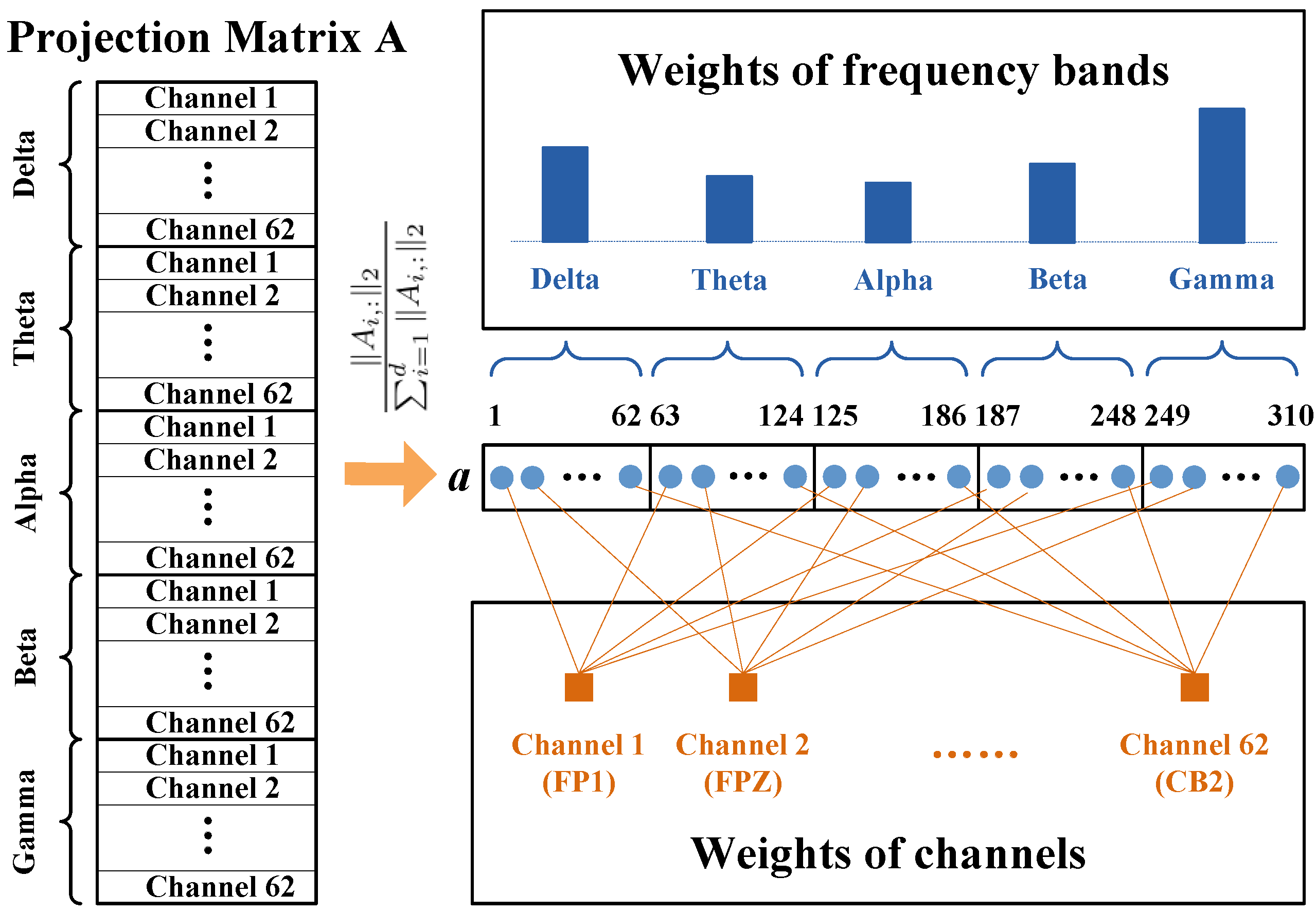
Due to the multi-rhythm and multi-channel properties of EEG, the sample vector is usually formed by concatenating spectra features extracted from different frequency bands. To be specific, the dimensionality $d=310$ of the SEED_IV dataset is obtained by each 62 points (corresponding to the 62 channels) of the 5 frequency bands (Delta, Theta, Alpha, Beta, and Gamma). Inspired by [35], the weight of each feature dimension can be quantitatively measured by the normalized ${\ell }_2$-norm of each row of the projection matrices. Taking $\mathit{A}\in {\mathbb{R}}^{d\times d_f}$ for example, if we use ${\mathit{a}}_i$ to denote the weight of the i-th EEG feature, it can be calculated as ${\mathit{a}}_i=\frac{\parallel {\mathit{A}}_{i,:}{\parallel }_2}{{\sum }_{j=1}^{310}\parallel {\mathit{A}}_{j,:}{\parallel }_2}$. Here ${\mathit{A}}_{i,:}$ is the i-th row of $\mathit{A}$ and its ${\ell }_2$-norm is defined by $\parallel {\mathit{A}}_{i,:}{\parallel }_2=\sqrt{{\sum }_{j=1}^{d_f}{\mathit{A}}_{ij}^2}$.

Once the feature weight vector $\mathit{a}=[{\mathit{a}}_1,{\mathit{a}}_2,\cdots ,{\mathit{a}}_{310}]$ is obtained, we can establish the correspondence between EEG features and frequency bands (channels) in Figure 9. Then, the importance of each frequency band can be measured by summing over the weight of EEG features belonging to such frequency bands; that is,

$${\mathit{w}}_j^{band}=\sum _{i=1}^{62}{\mathit{a}}_{(j-1)\times 62+i},j=1,2,3,4,5,$$

(23)

where $j=1,2,3,4,5$, respectively, denote the five frequency bands, Delta, Theta, Alpha, Beta, and Gamma. Similarly, the importance of the k-th EEG channel is

$${\mathit{w}}_k^{channel}=\sum _{i=1}^5{\mathit{a}}_{(i-1)\times 62+k},k=1,2,\cdots ,62.$$

(24)

The channel order can be found from the SEED_IV website.

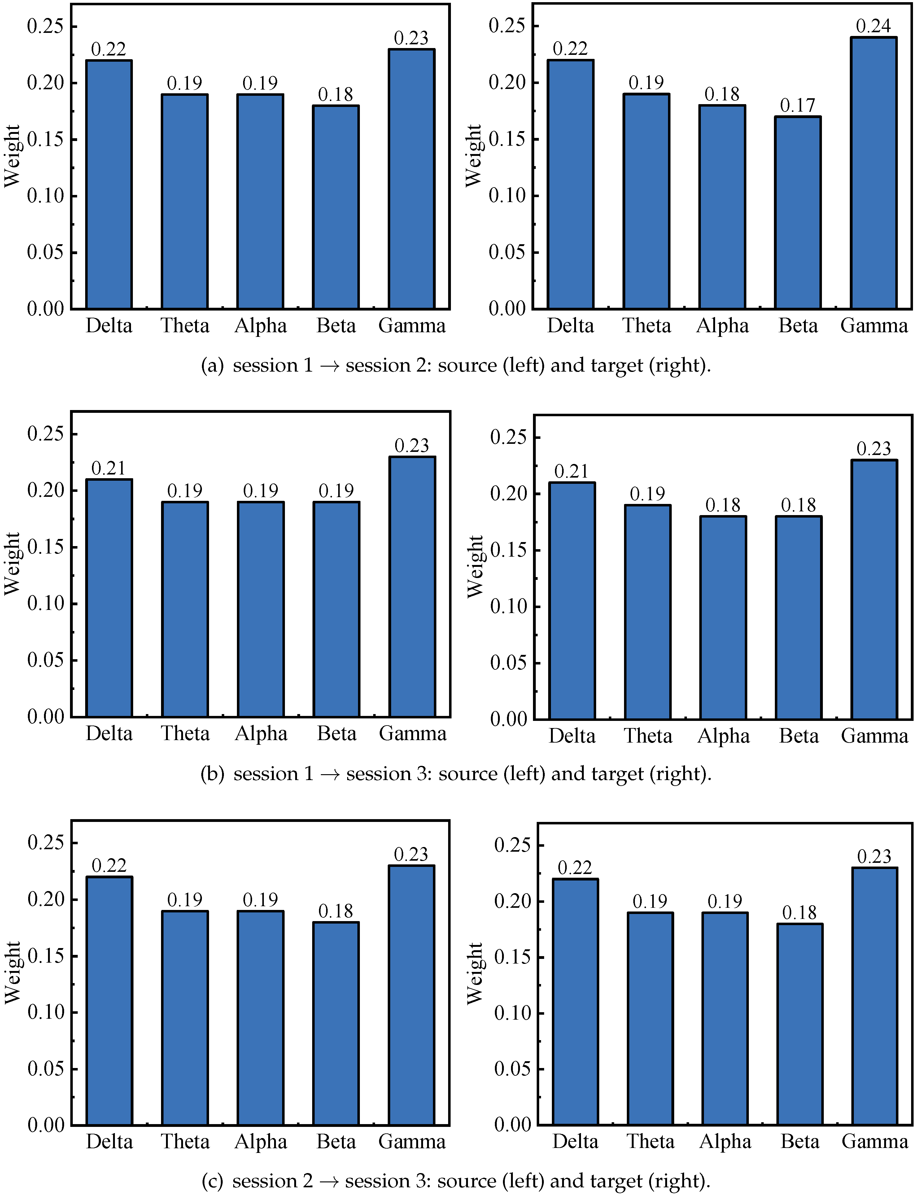
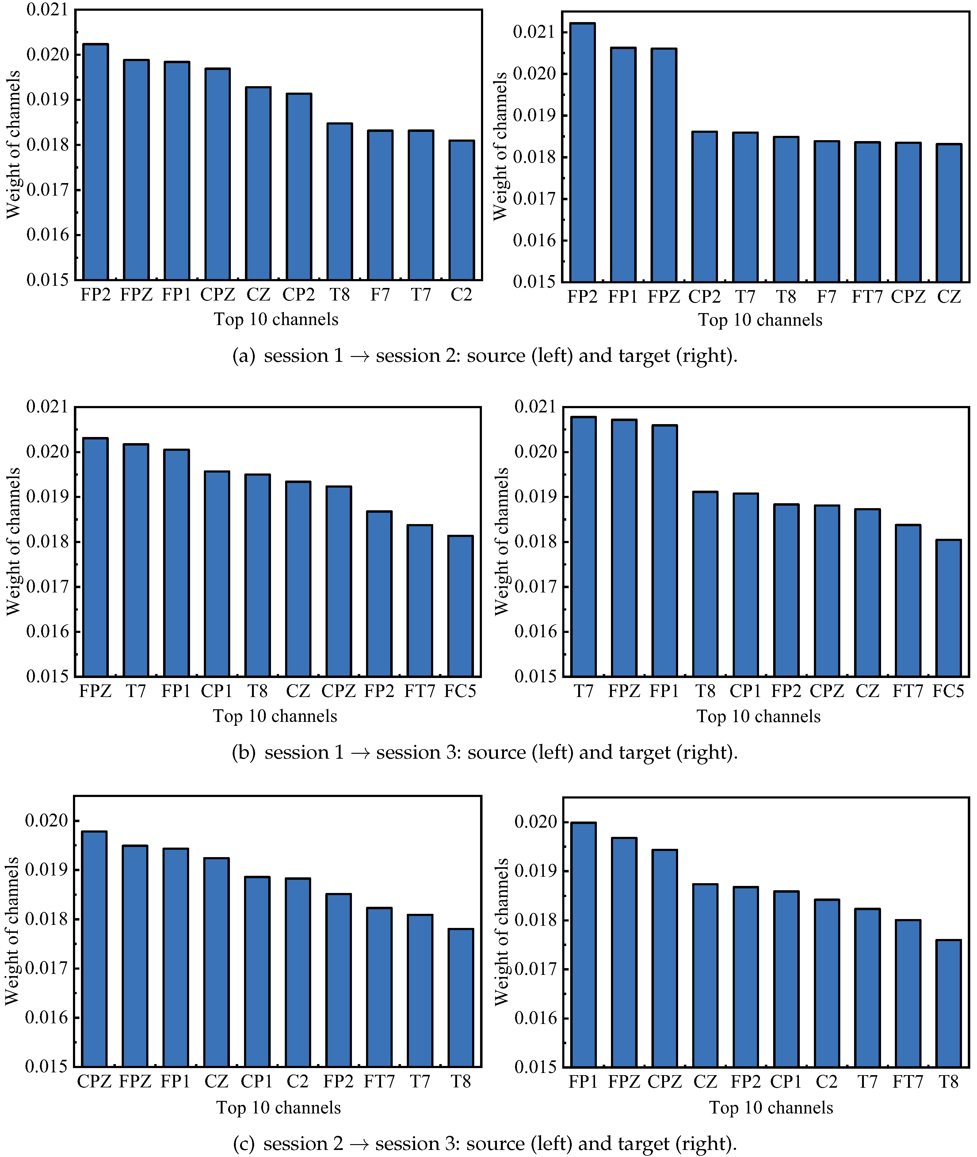
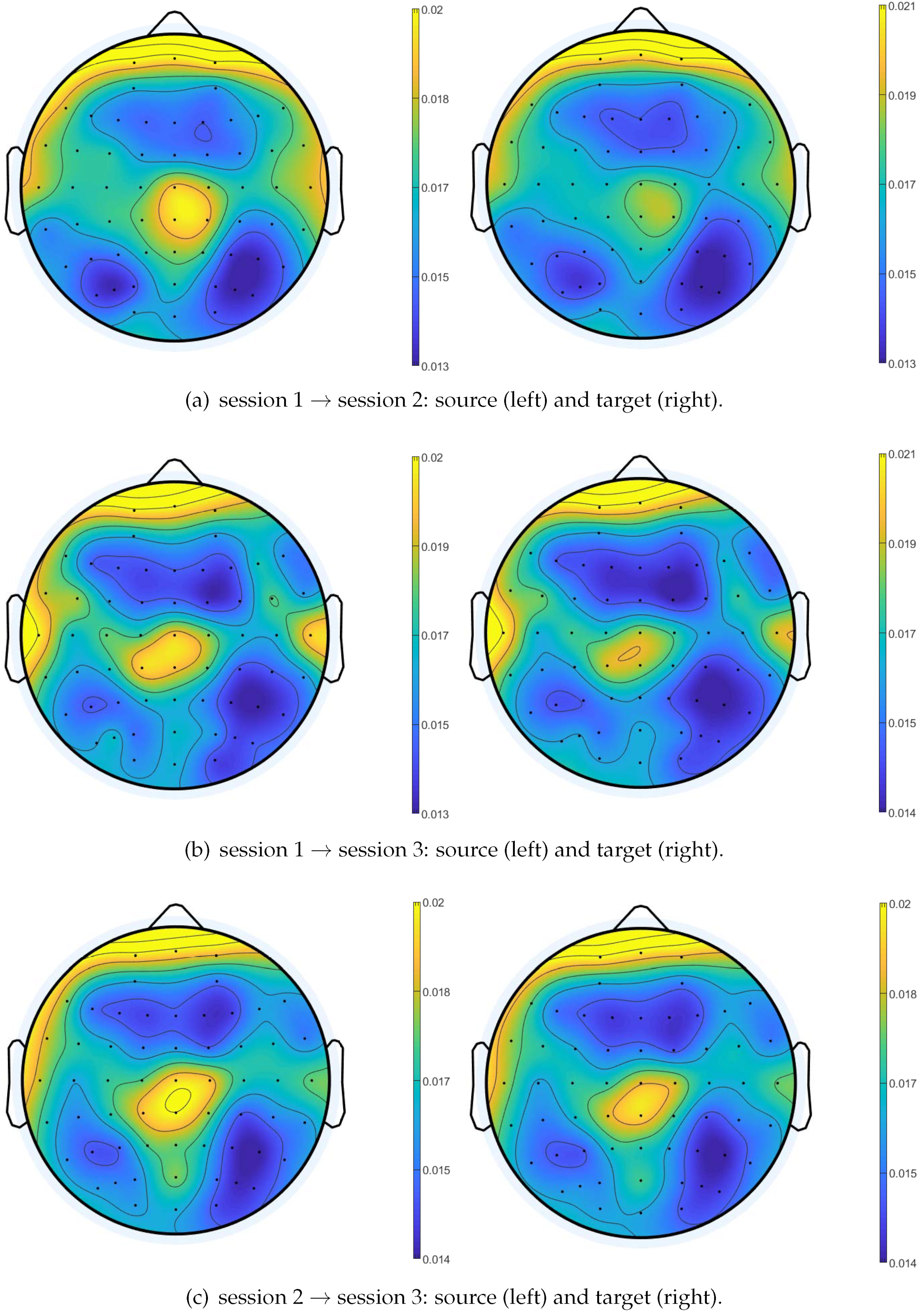
After obtaining the learned projection matrices $\mathit{A}$ and $\mathit{B}$, the importance of EEG frequency bands and channels in both source and target domains is achieved. According to Equation (23), the weight of frequency bands of both source and target domains are shown in Figure 10. From this figure, we observe that in all cases, the frequency band importance ranking of the source domain is consistent with that of the target domain. Further, the Gamma band has the greatest importance which is considered as the most important frequency band in EEG emotion recognition. This result also coincides with some previous studies [36,37]. Additionally, we calculate the importance of all channels by Equation (24), and the top 10 important channels of both source and target domains are shown in Figure 11. We observe that FP1, FPZ, CPZ, CZ, FP2, T7 and T8 channels are selected in all cases, meaning that these channels are important for cross-session emotion recognition. To be more intuitive, we transform the weight of all channels into the form of brain topographical map, where yellow color denotes significant brain regions, as shown in Figure 12. From it, we find that the channels in the prefrontal, left/right temporal and central parietal lobes have larger weights. This finding is consistent with previous research [38,39]. Based on the above observations, we conclude that our proposed CPTML model can effectively perform emotion knowledge discovery on critical EEG frequency bands and channels which are more powerful in cross-session emotion expression.

4. Conclusions

In this paper, we proposed a CPTML model to simultaneously minimize the cross-session and the cross-trial data discrepancies for EEG emotion recognition. Extensive experiments on the SEED_IV dataset demonstrated that (1) CPTML achieved better recognition performance then the other models by jointly taking into consideration the domain alignment and the graph-based metric learning. (2) In the coupled projection matrices-induced subspaces by CPTML, data distributions between the source and target domains were well aligned. Additionally, in the learned emotion metric graph, the connections of EEG samples from different trials but with the same emotional state have been significantly enhanced. (3) The Gamma frequency band and the brain regions of pre-frontal, left/right temporal and central parietal lobes were identified by CPTML as the more important ones in cross-session emotion expression.

References

- Chen, L.; Wu, M.; Pedrycz, W.; Hirota, K. Emotion Recognition and Understanding for Emotional Human-Robot Interaction Systems; Springer Nature: Berlin/Heidelberg, Germany, 2020; pp. 1–247. [Google Scholar]
- Papero, D.; Frost, R.; Havstad, L.; Noone, R. Natural systems thinking and the human family. Systems 2018, 6, 19. [Google Scholar] [CrossRef] [Green Version]
- Alarcao, S.M.; Fonseca, M.J. Emotions recognition using EEG signals: A survey. IEEE Trans. Affect. Comput. 2017, 10, 374–393. [Google Scholar] [CrossRef]
- Hondrou, C.; Caridakis, G. Affective, natural interaction using EEG: Sensors, application and future directions. In Proceedings of the Hellenic Conference on Artificial Intelligence, Ioannina, Greece, 15–17 May 2012; pp. 331–338. [Google Scholar]
- Marei, A.; Yoon, S.A.; Yoo, J.U.; Richman, T.; Noushad, N.; Miller, K.; Shim, J. Designing feedback systems: Examining a feedback approach to facilitation in an online asynchronous professional development course for high school science teachers. Systems 2021, 9, 10. [Google Scholar] [CrossRef]
- Mammone, N.; De Salvo, S.; Bonanno, L.; Ieracitano, C.; Marino, S. Brain Network Analysis of Compressive Sensed High-Density EEG Signals in AD and MCI Subjects. IEEE Trans. Ind. Inform. 2018, 15, 527–536. [Google Scholar] [CrossRef]
- Bhatti, M.H.; Khan, J.; Khan, M.U.G.; Iqbal, R.; Aloqaily, M.; Jararweh, Y.; Gupta, B. Soft computing-based EEG classification by optimal feature selection and neural networks. IEEE Trans. Ind. Inform. 2019, 15, 5747–5754. [Google Scholar] [CrossRef]
- Shen, F.; Peng, Y.; Kong, W.; Dai, G. Multi-scale frequency bands ensemble learning for EEG-based emotion recognition. Sensors 2021, 21, 1262. [Google Scholar] [CrossRef]
- Gao, Z.; Li, Y.; Yang, Y.; Dong, N.; Yang, X.; Grebogi, C. A coincidence-filtering-based approach for CNNs in EEG-based recognition. IEEE Trans. Ind. Inform. 2019, 16, 7159–7167. [Google Scholar] [CrossRef]
- Jayaram, V.; Alamgir, M.; Altun, Y.; Scholkopf, B.; Grosse-Wentrup, M. Transfer learning in brain-computer interfaces. IEEE Comput. Intell. Mag. 2016, 11, 20–31. [Google Scholar] [CrossRef] [Green Version]
- Zheng, W.L.; Liu, W.; Lu, Y.; Lu, B.-L.; Cichocki, A. EmotionMeter: A multimodal framework for recognizing human emotions. IEEE Trans. Cybern. 2018, 49, 1110–1122. [Google Scholar] [CrossRef]
- Pan, S.J.; Yang, Q. A survey on transfer learning. IEEE Trans. Knowl. Data Eng. 2009, 22, 1345–1359. [Google Scholar] [CrossRef]
- Zheng, W.L.; Lu, B.-L. Personalizing EEG-based affective models with transfer learning. In Proceedings of the Twenty-Fifth International Joint Conference on Artificial Intelligence, New York, NY, USA, 9–15 July 2016; pp. 2732–2738. [Google Scholar]
- Li, J.; Qiu, S.; Du, C.; Wang, Y.; He, H. Domain adaptation for EEG emotion recognition based on latent representation similarity. IEEE Trans. Cognit. Develop. Syst. 2019, 12, 344–353. [Google Scholar] [CrossRef]
- Nie, F.; Wang, X.; Huang, H. Clustering and projected clustering with adaptive neighbors. In Proceedings of the 20th ACM SIGKDD International Conference on Knowledge Discovery and Data Mining, New York, NY, USA, 24–27 August 2014; pp. 977–986. [Google Scholar]
- Wang, X.; Nie, F.; Huang, H. Structured Doubly Stochastic Matrix for Graph Based Clustering: Structured Doubly Stochastic Matrix. In Proceedings of the 22nd ACM SIGKDD International Conference on Knowledge Discovery and Data Mining, San Francisco, CA, USA, 13–17 August 2016; pp. 1245–1254. [Google Scholar]
- Cui, J.; Liu, Y.; Lan, Z.; Sourina, O.; Müller-Wittig, W. EEG-based cross-subject driver drowsiness recognition with interpretable convolutional neural network. IEEE Trans. Neural Netw. Learn. Syst. 2022. [Google Scholar] [CrossRef]
- Schölkopf, B.; Platt, J.; Hofmann, T. A kernel method for the Two-Sample-Problem. In Proceedings of the Advances in Neural Information Processing Systems, Vancouver, BC, Canada, 3–5 December 2007; pp. 513–520. [Google Scholar]
- Long, M.; Wang, J.; Ding, G.; Sun, J.; Yu, P.S. Transfer feature learning with joint distribution adaptation. In Proceedings of the 2013 IEEE International Conference on Computer Vision (ICCV), Sydney, Australia, 1–8 December 2013; pp. 2200–2207. [Google Scholar]
- Zhang, L.; Fu, J.; Wang, S.; Zhang, D.; Dong, Z.; Chen, C.L.P. Guide subspace learning for unsupervised domain adaptation. IEEE Trans. Neural Netw. Learn. Syst. 2019, 31, 3374–3388. [Google Scholar] [CrossRef]
- Li, J.; Wu, Y.; Zhao, J.; Lu, K. Low-rank discriminant embedding for multiview learning. IEEE Trans. Cybern. 2016, 47, 3516–3529. [Google Scholar] [CrossRef]
- Li, J.; Jing, M.; Lu, K.; Zhu, L.; Shen, H. Locality preserving joint transfer for domain adaptation. IEEE Trans. Image Process. 2019, 28, 6103–6115. [Google Scholar] [CrossRef] [Green Version]
- Yan, S.; Xu, D.; Zhang, B.; Zhang, H.J.; Yang, Q.; Lin, S. Graph Embedding and Extensions: A General Framework for Dimensionality Reduction. IEEE Trans. Pattern Anal. Mach. Intell. 2007, 29, 40–51. [Google Scholar] [CrossRef] [Green Version]
- Zhang, J.; Li, W.; Ogunbona, P. Joint geometrical and statistical alignment for visual domain adaptation. In Proceedings of the IEEE Conference on Computer Vision and Pattern Recognition, Honolulu, HI, USA, 21–26 July 2017; pp. 1859–1867. [Google Scholar]
- Ghifary, M.; Balduzzi, D.; Kleijn, W.B.; Zhang, M. Scatter component analysis: A unified framework for domain adaptation and domain generalization. IEEE Trans. Pattern Anal. Mach. Intell. 2016, 39, 1414–1430. [Google Scholar] [CrossRef] [Green Version]
- Shi, L.C.; Jiao, Y.Y.; Lu, B.-L. Differential entropy feature for EEG-based vigilance estimation. In Proceedings of the IEEE Engineering in Medicine and Biology Society, Osaka, Japan, 3–7 July 2013; pp. 6627–6630. [Google Scholar]
- Duan, R.; Zhu, J.; Lu, B.-L. Differential entropy feature for EEG-based emotion classification. In Proceedings of the International IEEE/EMBS Conference on Neural Engineering, San Diego, CA, USA, 6–8 November 2013; pp. 81–84. [Google Scholar]
- Sun, B.; Saenko, K. Subspace distribution alignment for unsupervised domain adaptation. In Proceedings of the British Machine Vision Conference, Swansea, UK, 7–10 September 2015; pp. 1–10. [Google Scholar]
- Peng, Y.; Li, Q.; Kong, W.; Qin, F.; Zhang, J.; Cichocki, A. A joint optimization framework to semi-supervised RVFL and ELM networks for efficient data classification. Appl. Soft. Comput. 2020, 97, 106756. [Google Scholar] [CrossRef]
- Wang, W.; Peng, Y.; Kong, W. EEG-Based Emotion Recognition via Joint Domain Adaptation and Semi-supervised RVFL Network. In Proceedings of the International Conference on Intelligent Automation and Soft Computing, Chicago, IL, USA, 28–30 May 2021; pp. 413–422. [Google Scholar]
- Friedman, M. The use of ranks to avoid the assumption of normality implicit in the analysis of variance. J. Am. Statist. Assoc. 1937, 32, 675–701. [Google Scholar] [CrossRef]
- Zhou, Z. Machine Learning; Tsinghua University Press: Beijing, China, 2016. [Google Scholar]
- Demšar, J. Statistical comparisons of classifiers over multiple data sets. J. Mach. Learn. Res. 2006, 7, 1–30. [Google Scholar]
- Van der Maaten, L.; Hinton, G. Visualizing data using t-SNE. J. Mach. Learn. Res. 2008, 9, 2579–2605. [Google Scholar]
- Nie, F.; Huang, H.; Cai, X.; Ding, C. Efficient and robust feature selection via joint ℓ2,1-norms minimization. In Proceedings of the Advances in Neural Information Processing Systems, Hyatt Regency, VC, Canada, 6–11 December 2010; pp. 1813–1821. [Google Scholar]
- Zheng, W.L.; Lu, B.-L. Investigating critical frequency bands and channels for EEG-based emotion recognition with deep neural networks. IEEE Trans. Auton. Ment. Develop. 2015, 7, 162–175. [Google Scholar] [CrossRef]
- Peng, Y.; Lu, B.-L. Discriminative manifold extreme learning machine and applications to image and EEG signal classification. Neurocomputing 2016, 174, 265–277. [Google Scholar] [CrossRef]
- Peng, Y.; Qin, F.; Kong, W.; Ge, Y.; Nie, F.; Cichocki, A. GFIL: A Unified Framework for the Importance Analysis of Features, Frequency Bands and Channels in EEG-based Emotion Recognition. IEEE Trans. Cognit. Develop. Syst. 2021. [Google Scholar] [CrossRef]
- Zhong, P.; Wang, D.; Miao, C. EEG-based emotion recognition using regularized graph neural networks. IEEE Trans. Affect. Comput. 2020. [Google Scholar] [CrossRef]
Figure 1.
The flow chart of EEG-based emotion recognition system.
Figure 2.
The distribution discrepancies between EEG from different sessions.
Figure 3.
The emotion metric graph of EEG samples from different trials.
Figure 4.
The overall framework of CPTML.
Figure 5.
Friedman test result of the five models.
Figure 6.
The average confusion graph of CPTML for cross-session EEG emotion recognition.
Figure 7.
We take subject 5 as an example to visualize the effect of data alignment by CPTML. Source and target domain samples are, respectively, marked as blue and red. Different shapes denote different emotional states.
Figure 8.
The emotion metric graph learned by CPTML on subject 5.
Figure 9.
The correspondence between the projection matrix and the weight of frequency bands (channels).
Figure 10.
The importance of frequency bands corresponding to source (left) and target (right) domains.
Figure 11.
The top 10 EEG channels corresponding to source (left) and target (right) domains.
Figure 12.
The importance of EEG channels corresponding to source (left) and target (right) domains in the form of a brain topographical map.