Article

Sustainability Assessment of Asset Management Decisions for Wastewater Infrastructure Systems—Development of a System Dynamic Model

by
Hamed Mohammadifardi
1,
Mark A. Knight
1,2,* and
Andre A.J. Unger
3
1
Center for Advancement of Trenchless Technology (CATT), University of Waterloo, 200 University Avenue, Waterloo, ON N2L 3G1, Canada
2
Department of Civil and Environmental Engineering, University of Waterloo, 200 University Avenue, Waterloo, ON N2L 3G1, Canada
3
Department of Earth and Environmental Sciences, University of Waterloo, 200 University Avenue, Waterloo, ON N2L 3G1, Canada
*
Author to whom correspondence should be addressed.
Submission received: 2 March 2019 / Revised: 26 April 2019 / Accepted: 9 May 2019 / Published: 13 May 2019

Abstract

:
This paper presents the development of a novel system dynamics (SD) model for better understanding the interrelation and feedback mechanism between the wastewater collection (WWC) and wastewater treatment plant (WWTP) systems. Causal loop diagrams (CLDs) are developed and discussed to depict and understand feedback and inter-connections between physical, financial, and consumer sectors. The developed SD model is then extended to include the greenhouse gas (GHG) emissions, as a proxy for the environmental sector and for an environmental sustainability assessment of strategic decisions related to asset management planning of wastewater infrastructure system. It also adds new policy levers, such as population growth and urban densification in the social sector, and minimum fee-hike rates in the finance sector to enhance the representation of real-world conditions in the asset management planning. This new SD model will enable decision-makers to assess the sustainability impacts of their strategic decisions on wastewater systems, find synergistic cost-saving opportunities, and improve the sustainability performance of their asset management plans.

1. Introduction

The government of Canada has committed to and established strategic objectives to move the country toward economic, social, and environmental sustainable development. As one step, it appointed an advisory council and constituted an office for the development and implementation of the Federal Sustainable Development Act [1]. More recently, the Federal Sustainable Development Strategy [2] has been developed as a vehicle for planning and reporting to the government of Canada the sustainable development priorities, goals, and actions from 41 federal organizations. The government’s strategies have further trickled down into various jurisdictions and organizations, including civil and environmental engineering. In particular, leadership in sustainable infrastructure development has become one of the three main strategic goals of the Canadian Society of Civil Engineering [3].
In addition to the increasing interest in sustainable development, the intrinsic need to rejuvenate deteriorated urban infrastructure has motivated sustainable urban infrastructure planning. Specifically, the Federation of Canadian Municipalities (FCM) has promoted a guidebook [4] under the Leadership in Asset Management Program (LAMP), to support municipalities in integrating sustainability considerations into their asset management policies and strategic plans [5]. These legislative frameworks and guidelines are leveraged by economic incentives and programs, such as the Green Municipal Fund [5] and the Municipalities for Climate Innovation Program [6] provided by FCM.
A specifically Canadian model framework is being developed by the National Round Table on Sustainable Infrastructure (NRTSI) and the National Research Council (NRC) to create a unified approach to assessing the condition state, performance, and management of the country’s core public infrastructure assets [7]. The International Standard Organization (ISO) provides definitions, standard requirements, and a checklist of good practices for developing asset management programs in its ISO-55000 series [8].
These retrospective assessment frameworks apply various indicators to “check” the performance of asset management plans on the continual ISO 55000 Plan–Do–Check–Act asset management cycle (Figure 1). This will help decision makers to act upon deficiencies found in the previous planning cycle. However, such frameworks are not specifically designed to appraise the future performance of asset management decisions. Therefore, “sustainability assessment” tools are needed to project the performance of assets onto their future life-cycle and to inform decision makers to develop sustainable asset management plans in an iterative process.
Commercial software such as RIVA, Hansen, InfraModex, MIMS, Synergen, IBM Maximo, Infrastructure 200, and Harfan are examples of existing software packages used in the corporate asset management industry. The majority of these tools focus on day-to-day work-order planning at the operational level, and are rarely developed to support long-term and strategic life-cycle asset management planning [9].
A complete sustainability assessment, should assess all dimensions of sustainability (i.e., economic, social, environmental), deal with non-linearity and dynamic features, have a system-wide perspective to include all life-cycle stages, support scenario development, and include the consequences on upstream and downstream processes (i.e., water distribution (WD) and wastewater treatment plant (WWTP) systems, respectively) [10]. However, the current studies on sustainable asset management planning often consider the environmental, economic, and social components related to urban water and wastewater in isolation from one another. Moreover, the dynamic interactions and feedback between urban water and wastewater systems are not considered in current sustainability assessment approaches [11].
The overall goal of this paper is to develop the system dynamics (SD) model of integrated wastewater collection (WWC) and WWTP system presented by Mohammadifardi et al. [12] for sustainability assessment of wastewater asset management plans. To achieve this objective, causal loop diagrams (CLDs) are developed to demonstrate the interconnections and feedback mechanisms between the different components of the physical, economic, consumer, and environmental sectors related to WWC and WWTP systems. Then, the conceptual CLDs is been parametrized with data collected from several small to medium size municipalities in southern Ontario.

2. Review of SD Models of Water Infrastructure System

SD is a versatile tool for modeling and assessing the socio-economic impacts of implementing strategic decisions. It was developed by Jay Wright Forrester during the mid-1950s, and has often been applied as a convenient simulation tool for modeling the socio-economic impacts of strategic decisions on water resource management problems [13].
Recently, SD has been used to model the complexity of water and wastewater infrastructure systems. Chung et al. [14] applied SD to model water sources, users, recharge facilities, and water and WWTP as subsystems for general water supply planning, and to calculate the construction, operation, and maintenance costs of water and WWTPs. Biachia and Montemaggiore [15] integrated SD with the “balanced scorecard” approach to analyze the dynamics and interdependencies between key financial indicators and intangible variables, such as the customer satisfaction, business image, and bargaining power of a water utility company.
SD modeling is also being used as an optimization technique for designing WWTP systems—see studies done by Das et al. [16], Gillot et al. [17], and Parkinson et al. [18]. These studies demonstrate the dynamics and complexity of wastewater treatment (WWT) systems and present feedback mechanisms between different components of a WWTP system at the operational level.
Rehan [19] and Rehan et al. [20,21] developed the first known SD model to evaluate the financial sustainability of urban WD and WWC systems and showed various interconnections and feedback between the physical, financial, and social systems.
Ganjidoost [22] built on Rehan et al. [20,21] SD model by improving the financial model and adding feedbacks and interconnections mechanism between the WWC and WD systems. Ganjidoost et al. [23] proposes a set of normalized and time-integrated “benchmarking performance Indicators” for sustainable long-term management of WD and WWC networks. The benchmarking performance indicators are aggregated into three categories: (1) infrastructure, (2) socio-political, and (3) financial. To demonstrate the use and value of the benchmarking performance indicators, the advanced Rehan et al. [24] SD model for water distribution networks was used to forecast the future performance of each utility. Policy levers controlling the forecasting exercise were made as identical as possible between each utility under the assumption they will have similar preferences (due in part to their geographic proximity) for strategic targets, policy levers, sustainability, and life-cycle. For this study a pay-as-you-go financing strategy is considered over a 100-year life-cycle of the infrastructure system representing the benchmarking period.
Both Rehan [19] and Ganjidoost [22] applied SD modeling approach for simulation of the future condition of pipe-network systems and projection of subordinated operational and capital costs to evaluate management strategies for rehabilitating and replacing urban water and wastewater pipe-network systems. They also considered water treatment as an exogenous input value and did not consider population growth and urban densification.
To better model an integrated water and wastewater infrastructure system, the model should include both the linear water distribution and WWC networks and the non-linear water and WWT systems, as illustrated in Figure 2.

3. Ganjidoost SD Model Advancement

In this study, the Ganjidoost et al. [25] physical, social, and finance sectors of the WWC asset management planning model is updated to include: (1) population growth, (2) urban development, (3) WWTPs’ physical and financial models, and (4) energy footprint and greenhouse gas (GHG) emission modules as proxy indicators for environmental sustainability assessment. Details on the model advancement are presented in the following sections.

3.1. CLD Development

This section explores the interactions and feedback between WWC and WWTP systems and presents CLDs for different sectors such as the consumer, physical, financial, and environmental.
The total inflow volume received by a WWTP depends on the volume of inflow and infiltration (I&I) entering into the WWC pipe network system, and the volume of sewage generated by system users. While the revenue of the WWTP sector is generated based on consumers’ metered water, its operational expenses are based on the fraction of metered water plus the extraneous inflow and infiltration (I&I). Rehan et al. [26] showed that the I&I makes a significant contribution to wastewater volume; on average, the monthly volume of collected wastewater is 25% higher than the corresponding volume of metered water, and at peak-flow exceeds it by 74% [26].
The infiltration rate to the WWC pipe network system increases as WWC pipes deteriorate and their internal condition grade increases. Sewage generation is increased by population growth, which also affects the I&I flow rate due to WWC pipe network expansion in urban area development. The consequence of an increasing inflow volume is an increasing cost of operating WWTPs, and the need for capital investment to expand capacity. In contrast, it is assumed that decommissioning a WWTP will have no significant capital cost. Construction and operation of new WWTP capacities, as well as, the installation and operation of extended WWC pipe network will increase the energy footprint of the whole system.
To increase the fund balance, utilities need to increase revenues by increasing user fees. Since the wastewater collection and treatment fees are directly related to the metered volume of water, the response of users will be water-demand reduction which leads to a decrease of the energy footprint by reducing the energy-use in upstream water treatment and water distribution systems. Population growth will also increase the user-fee based revenues of WWC and WWT utilities. Development charges are another revenue stream for utilities, collected to cover the required capital work expenses due to urban development.
Qualitative relationships among the variables below are identified in CLDs, then parametrized in the SD model. Figure 3, Figure 4, Figure 5 and Figure 6 present the CLDs for the SD model of integrated WWC and WWTP systems.
Figure 3 reinforcing loop (R1) shows an increasing pipe deterioration rates increases the I&I flow rate which in turn decreases the pipes’ condition grade. Rehan [19] showed that the unit maintenance cost of the WWC pipes will increase with an increase in pipe condition grade. Reinforcing loop (R2) shows a decrease in the WWC pipes’ condition grade as the result of increasing operational expenditures, decreasing utilities’ fund balance, and, subsequently, decreasing available funds for rehabilitation of the WWC pipes. To increase the fund balance, WWC utilities need to increase revenues by increasing user fees. Since the WWC fees are directly related to the metered volume of water, the response of users will be water-demand reduction.
Reinforcing loop (R3) shows that users’ water-conservation efforts result in decreasing WWC revenues, which means less available funds for utilities to spend.
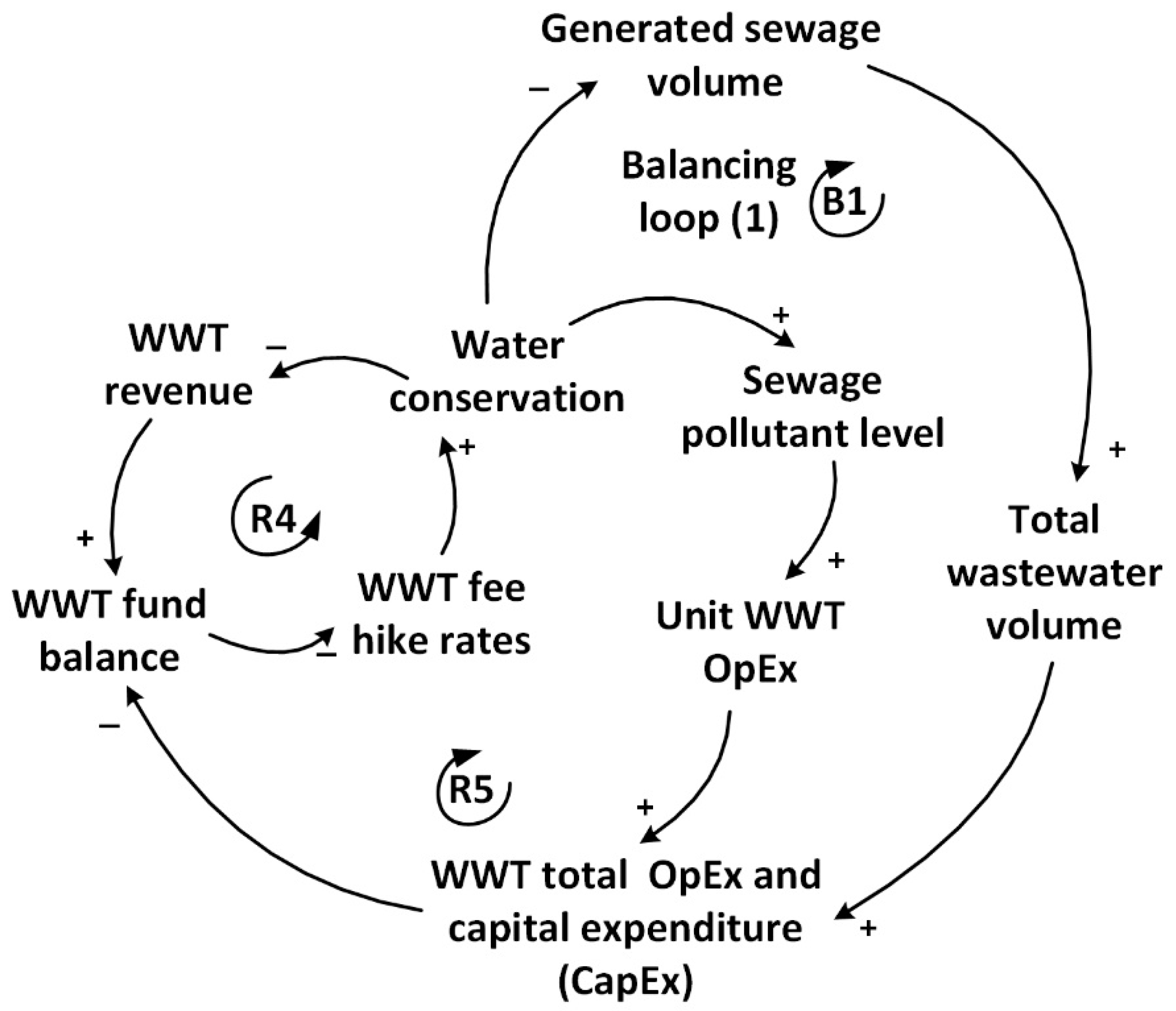
Figure 4 shows the CLD for WWTP system. Reinforcing loop (R4) shows that users’ water-conservation will result in decreasing WWT revenues and decreasing WWT fund balance. Parkinson et al. [18] have reported that an increase in the concentration of suspended solids (SS) and biological oxygen demand (BOD) in wastewater are a result of water-conservation scenarios. Min and Yeats [27] have shown an increase in the operational cost of WWC and WWT services as a result of BOD and SS level increases. DeZellar and Maier [28] argued that the total cost of WWT might be lower with a decrease of the total wastewater volume, but the unit cost of the operation and maintenance of WWTP increases due to non-routine operational problems such as clogging, changing bacterial activities, or malfunctioning of the biological treatment processes, and the extra chlorination and recirculation needed to prevent odor problems, etc.
Reinforcing loop (R5) shows the cause-and-effect-chain mechanism that exists between water conservation, sewage pollutant levels, operation, and maintenance costs of the WWTP systems, fund balances, and fee hikes.
Balancing loop (B1) shows that the reduction of total wastewater volume from water conservation will lower the operational and capital expenses and increase the fund balance. The increase of the fund balance will reduce the service-fee-increase rate, leading to a decrease in water conservation.
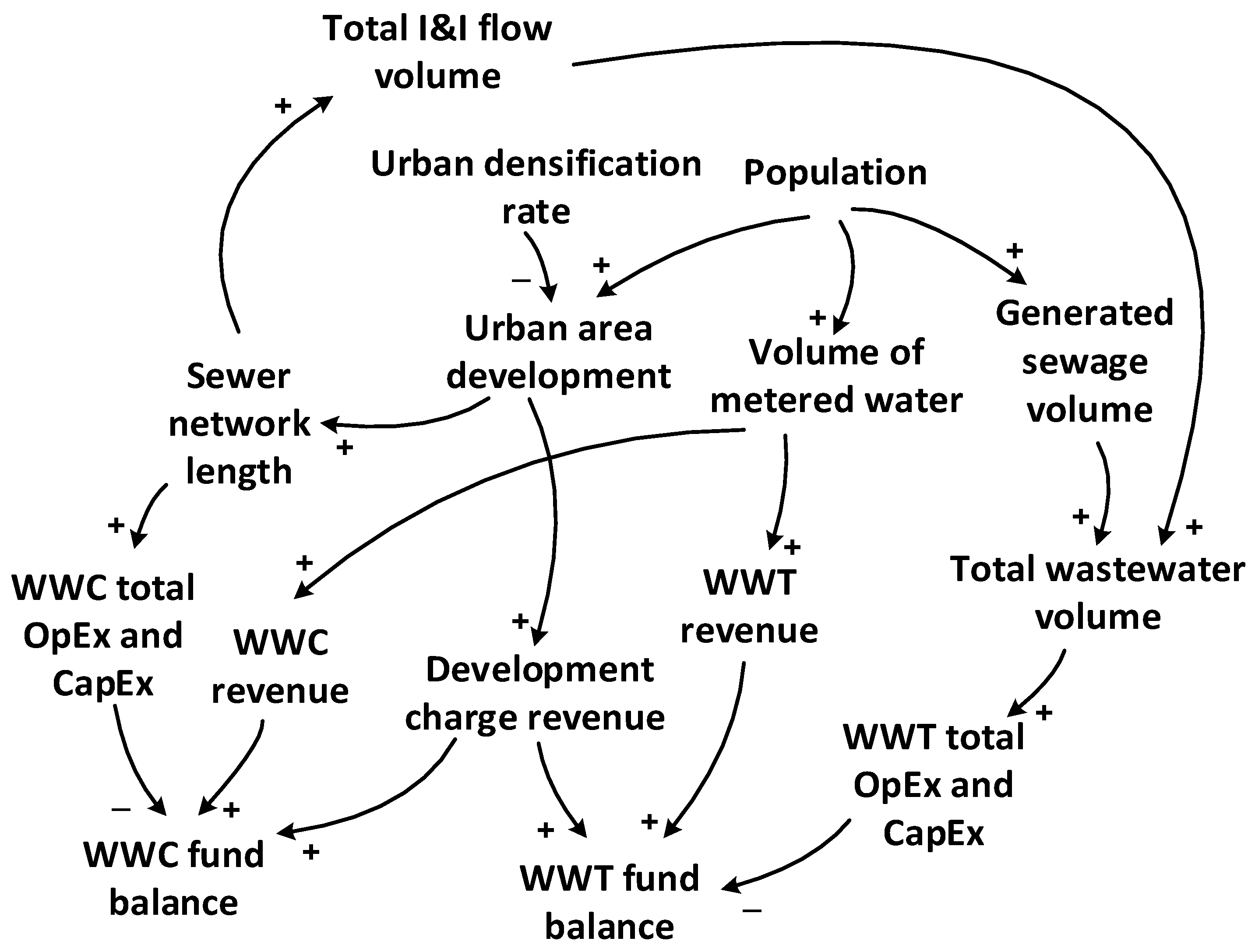
Figure 5 presents the interconnections between the WWC and WWTP systems. The total inflow volume received by a WWTP depends on the volume of inflow and infiltration (I&I) entering into the WWC pipe network system, and the volume of sewage generated by system users. While the revenue of the WWTP sector is generated based on consumers’ metered water, its operational expenses are based on the fraction of metered water plus the extraneous inflow and infiltration (I&I). Rehan et al. [26] showed that the I&I makes a significant contribution to wastewater volume as the monthly volume of collected wastewater is 25% higher than the corresponding volume of metered water, and at peak-flow exceeds it by 74%.
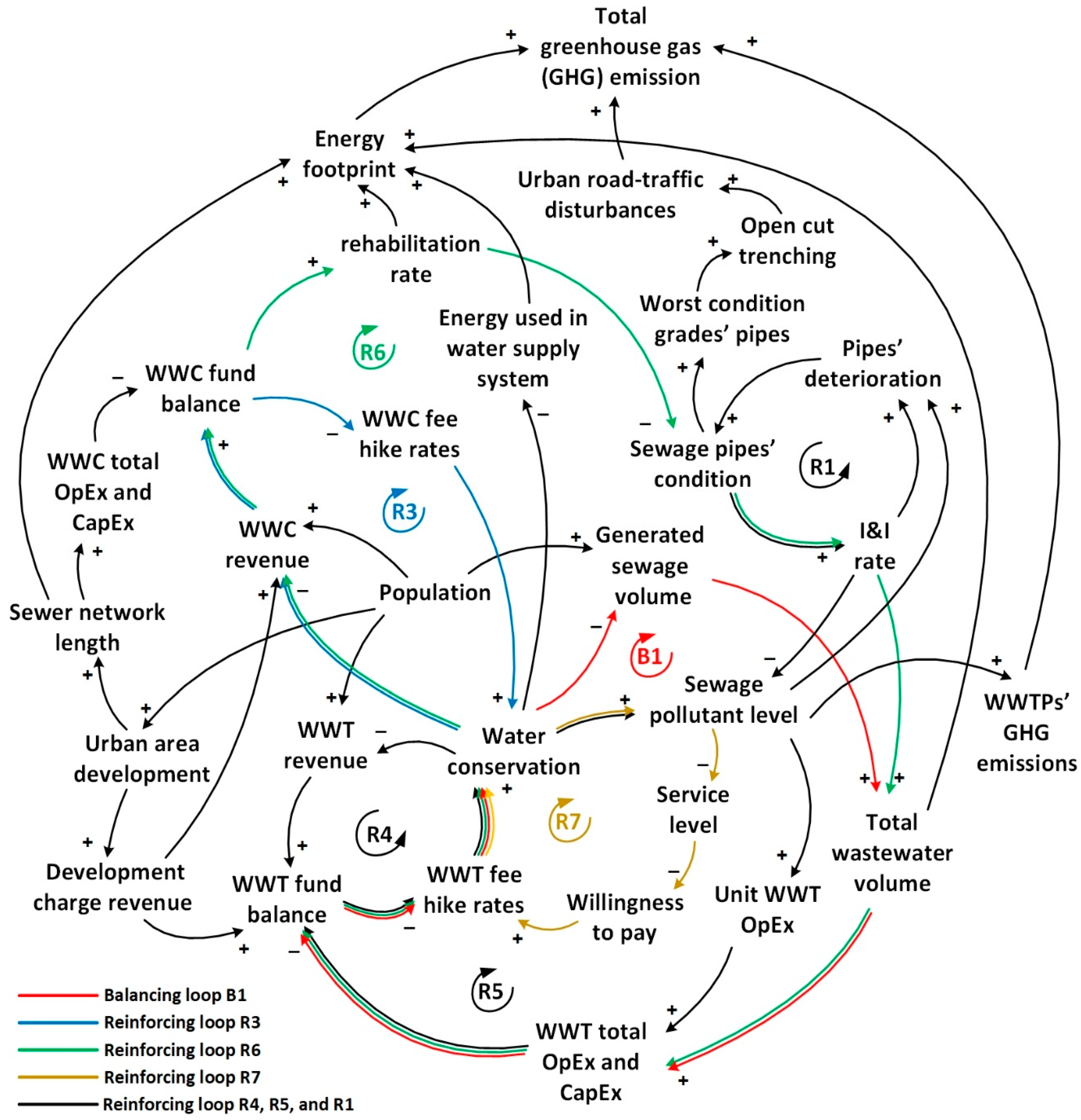
Reinforcing loop (R6) shows that increasing the WWT fee will increase the water conservation rate, which in turn cause reduces the WWC revenue and the funds available for reinvestment and rehabilitation of the WWC pipes. This in turn leads to further deterioration of a WWC pipes (increases the condition grade), which increases I&I flowing into the WWTPs.
Marleni et al. [29] demonstrated that water-use reduction in various water-demand management scenarios increases the concentration of sulfide and sulfate levels by 30% and 40%, respectively. These two compounds, which are the main source of hydrogen sulfide formation, will cause odor problems and corrosion of WWC pipes.
Reinforcing loop (R7) shows that the increased pollutant concentration, from water conservation, will increase WWC pipes’ blockages rate, resulting in reduced service performance of the wastewater pipe network, and increase the willingness of service users to accept WWT fee hikes and pay for service improvements.
Figure 6 shows impacts of population growth and urban densification on WWC and WWTP systems.
Growing population with urban development will cause the WWC pipe-network length to extend and incur capital and operational costs for both the WWC and WWTP utilities. Sewage generation will increase with population growth and the I&I flow rate will increase due to WWC pipe network expansion. On the revenue side, population growth will increase the user-fee based revenues for both WWC and WWT due to the increased volume of metered water. Development charges are collected from land developers to cover the required capital work expenses.
Figure 7 shows all developed interconnections and feedbacks (Figure 3, Figure 4, Figure 5 and Figure 6) between the WWTP and WWC physical, finance, and consumer sectors. It also depicts the related components contributing to GHG emissions from WWC and WWTP systems.
As discussed earlier, water conservation, as well as I&I reduction, will increase pollutant concentrations in wastewater. The increased BOD level will increase the methane gas yield as a main source of GHG emission from WWT processes [23]. Construction and operation of new WWTP capacities, as well as the installation and operation of extended WWC pipe network, will increase the energy footprint of the whole system. Replacement of highly deteriorated pipes (ICG5) by open-cut trenching technologies can lead to traffic delays and consequently more GHG emissions from cars’ engine-fuel combustion [30]. Water-demand reduction will also lead to a decrease in the energy footprint by reducing the energy-use in upstream water treatment and water distribution systems, which in turn will reduce GHG emission.

3.2. SD Model Parameterization

The Rehan [19] and Ganjidoost [22] developed their SD model using Stella® software, Research Version 9.1.4 [31]. The four basic elements, as in any SD model, are the stock, flow, converter, and connector. Stocks represent the accumulation of physical or non-physical elements in a system (e.g., the length of sewer pipes in worst condition grade (Sewers_Grade5) presented in Figure 8). Flows are used to model the inputs or outputs to the stock, and represent the activities in a system (e.g., the length of new wastewater pipes added to the network each year (New_WW_pipe_installation) presented in Figure 8). Converters are used to incorporate the effects of changing variables in an SD model (e.g., the value for the Population_Growth_rate presented in Figure 8); and, connectors represent the links between the convertors, stocks, and flow components of an SD model. The following section describes the SD model comprised of four sectors: (1) physical, (2) consumer, (3) finance, and (4) environment. It also presents new elements and changes made to the validated and calibrated models developed by Rehan et al. [20,21,26] and Ganjidoost [22] for WWC network system.

3.2.1. Physical Infrastructure Sector

This section provides a brief overview of the WWC pipe network SD model developed by Rehan, R. [19] followed by the new model development for the WWTP system.

WWC Physical Model

Pipe inventories are made up of different pipe materials such as vitrified clay, concrete, polyvinyl chloride (PVC), ductile iron, etc., and are grouped into five classes, which are represented in Figure 8 as stocks, based on their internal condition grade (ICG) as defined by the Water Research Center (WRc) in the United Kingdom [32]. The method used in Rehan et al. [26] is adapted to define the deterioration and infiltration rates.
New pipes with the best ICG are in the first stock class, whereas pipes in the worst condition belong to the fifth stock class. Today, PVC pipes are used in new pipe installation projects. Therefore, the new pipes, either for upgrading the ICG5 stock or for urban development and network expansion, are entered into the first PVC pipe stock.

WWTP Physical Model

The physical assets of WWTPs consist of electromechanical equipment, such as pumps, motors, aerators, mixers, tanks, basins, pipes, and buildings. 
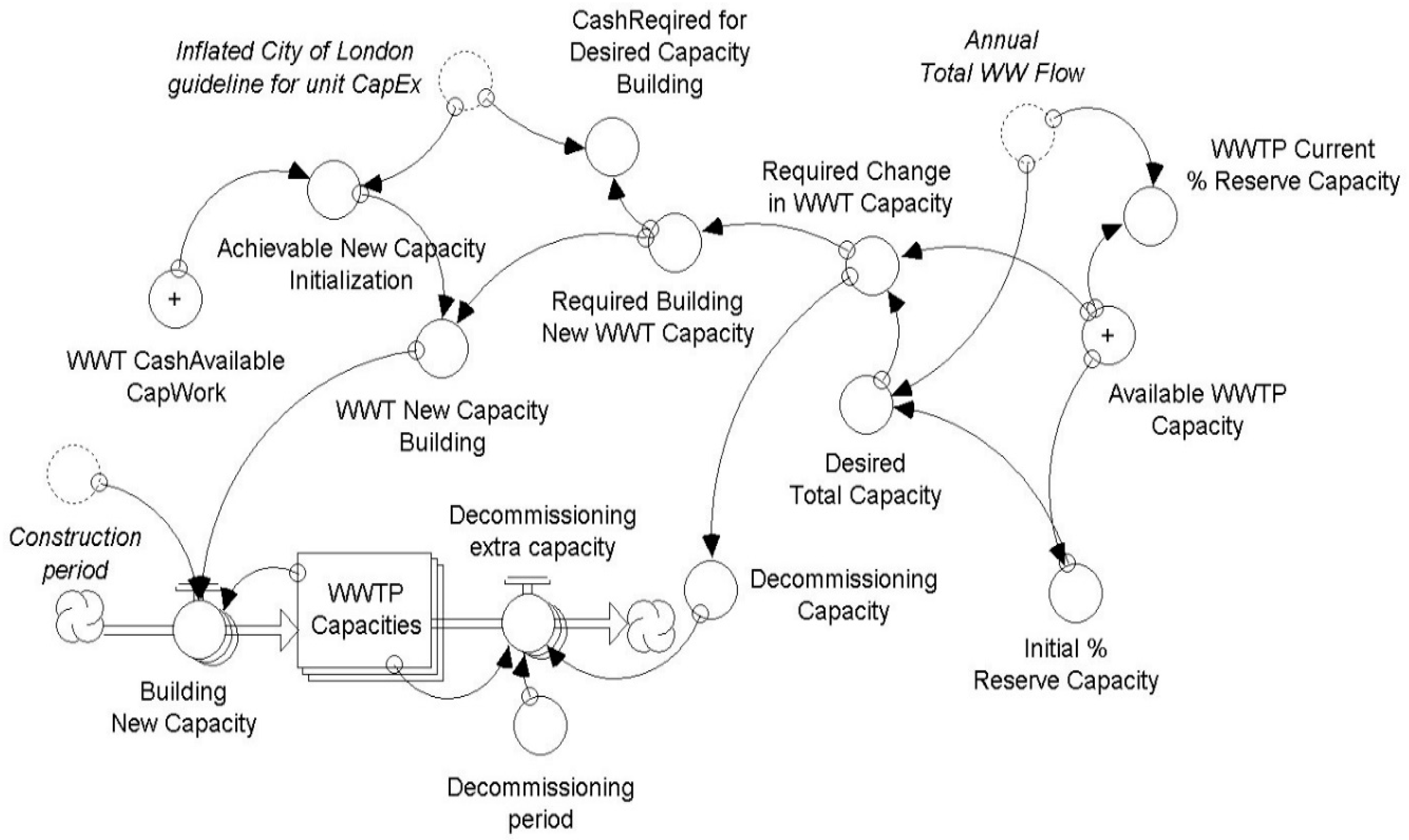
Figure 9 shows the modeling of WWTP assets at a strategic level, which is based on the WWTP capacity requirement.
The Required_Change_in_WWT_Capacity [m3/d] is equal with the difference between the Available_WWTP_Capacity [m3/d] and the Desired_Total_Capacity [m3/d], which is the sum of annual total wastewater flow (Annual_Total_WW_Flow [m3/d]) and the required reserve capacity (Initial_%_Reserve_Capacity [m3/d]).
The reserved capacity for the maximum seasonal, daily, and hourly peak wastewater flow can be estimated based on two methods: (1) the current reserve capacity of the WWTPs, or (2) based on the recommended standard defined by the Great Lake-Upper Mississippi River Board [33]. The desired reserve capacity in this model is calculated based on the initial percentage reserve capacity percentage, which is assumed to be maintained for the entire simulation period.
A positive difference indicates that capacity construction must be initiated (Required_Building_WWT_Capacity [m3/d]), whereas a negative difference suggests the decommissioning of extra capacities. The annual total wastewater flow is estimated based on the sewage generation from residential and non-residential users and the annual I&I flow. The sewage generation rate depends on the population growth rate and water demand rates, and the I&I flow rate depends on the WWC pipes’ conditions.

Wastewater Composition Model

The concentration of SS and BOD is assumed to increase proportionally with declining wastewater volume flowing into WWTPs. The unit mass of BOD and SS per capita is assumed to be fixed in time and is calculated based on the annual mass of BOD and SS reported by the WWTP divided by the current population. Thus, the concentration of SS and BOD changes as the generated wastewater—which is a function of the water demand (WD) and the consumptive use fraction (CUF) of metered water—and I&I change over the simulation period. The concentration of BOD and SS are formulated as in Equations (1) and (2), respectively.
SS (t) = ((SS0) × population (t))/(365/1000 × WD (t) × (1−CUF) × population (t) + I&I(t))
where
  • t [year] is the current time;
  • SS (t) [g/l] is the concentration of suspended solid in wastewater inflow at WWTP in year t;
  • SS0 [kg/capita/year] is the initial mass of suspended solid generation per capita;
  • 365/1000 [(day/year)/(m3/liter)] is the conversion factor to convert days to year and liter to cubic meter;
  • WD (t) [liter/capita/day] is the average daily water demand of a residential user in year t;
  • CUF [%] is the percentage of water received by customers that is not returned as sewage to the WWC pipe network;
  • I&I [m3/year] is the annual inflow and infiltration volume to the WWC pipe network;
  • Population (t) is the population number in year t.
BOD (t) = ((BOD0) × population (t))/(365/1000 × WD (t) × (1-CUF) × population (t) + I&I (t))
where
  • t [year] is the current time;
  • BOD [kg/capita/year] is the mass of dissolved oxygen needed by aerobic biological organisms to break down organic material presented in wastewater sample in year t;
  • BOD0 [kg/capita/year] is the initial BOD;
  • 365/1000 [(day/year)/(m3/liter)] is the conversion factor to convert days to year and liter to cubic meter;
  • WD (t) [liter/capita/day] is the average daily water demand of a residential user in year t;
  • CUF [%] is the percentage of water received by customers that is not returned as sewage to the WWC pipe network;
  • I&I [m3/year] is the annual inflow and infiltration volume to the WWC pipe network;
  • Population (t) is the population number in year t.

3.2.2. Consumer Sector

Consumers reactions to incremental change of wastewater service fees are modeled based on Ganjidoost [22] SD model. The daily water-use per capita or water demand is estimated as a function of the Price_Elasticity [-] of demand, User_Fee [$/m3], and Minimum_Water_Demand [liter/capita/day].
The price elasticity of demand, which is the percentage change in water demand per corresponding percentage change in the fee, is selected as −0.35, similar to the Rehan et al. [24] model. The minimum water demand is considered to be 150 liters per capita per day (LPCD) [26]. The modeling of the consumer sector is improved by decoupling non-residential and residential users, and by adding a population growth model. In Ganjidoost, A. [22] model, water demand is calculated as the sum of residential, commercial, institutional, and industrial water demand divided by population, under the assumption that all customers experience the same price elasticity of water demand. However, this assumption does not address that the industrial users can often apply technological means to reuse and conserve water and significantly cut their water demands. Water and wastewater utilities also set different price rates for non-residential users, in consideration of their social and economic importance to the societies who are depending on them. The water demands, wastewater collection, and treatment fees for non-residential users are assumed to be fixed in the present model.
The expanded SD model is deemed to better represents the projection of user-fee based revenues, user-fee hike rates, and the wastewater volume collected and treated in the WWC and WWT models. A policy favoring fixed wastewater service fees for non-residential users indicates a strategy, whereby residential users are subsidizing the system, and the result is a more stable economic sector. The wastewater collection and treatment services are subsidized for commercial, institutional, and industrial users if their fee increase rate is lower than the residential fee-hike rates and vice versa.
Population growth has been modeled by an urban densification index (UDI) to represent various urban development scenarios. In 100% urban densification (UDI = 100%) new population is served within the current WWC pipe network, which avoids the need to install and operate new pipes. It also does not impact the WWTP system’s operation and capacity planning due to future I&I to the new parts of the WWC pipe network. In contrast, a no urban densification scenario (UDI = 0%) requires a growing WWC pipe network, which would incur capital and operational costs for both the WWC and WWTP utilities.

3.2.3. Finance Sector

In this section, the models developed for the WWC and WWT finance sectors are described.

WWC Finance Model

Figure 10 presents the model developed for the WWC finance sector. The operation and maintenance cost of pipes in different ICG-categories and the user-fee calculation are modeled similar to the Rehan, R. [19] and Ganjidoost [22] SD models.
The revenues are generated from the WWC_Fee [$/m3] and WWC_Service_Charges [$/month]. The connection-service charges are based on the water-meter sizes and are collected monthly. The number of meters in each size is assumed to be increased by the same rate as the population growth rate. The service charges inflation is considered to be equal to the non-residential buildings construction-price-index (NRB CPI), which is reported as 3.7% per annum by Statistics Canada [34].
The new parts of the model consist of separate fund-balance stocks for operational and capital expenses, which are presented as WWC_Op_FundBalance [$] and WWC_Cap_FundBalance [$], respectively in Figure 10. In the advanced finance module, the generated revenues are primarily allocated to pay for the WWC_Maintenance_Expenses [$/year] and WWC_Debt_Services [$/year], and the remaining is transferred to the capital fund balance (WWC_Operation_Over_Fund [$/year]) for paying the capital costs of WWC pipe network rehabilitation and expansion.
The WWC utility has the option to issue debt to maintain a zero-capital fund balance if the revenue from operational fund balance is not sufficient to pay the capital expenses. In the opposite scenario, the surplus revenue can be reserved for future capital expenses. Separation of the two fund balance accounts in the present model restricts payment for operational expenses from issued debt or reserved cash.
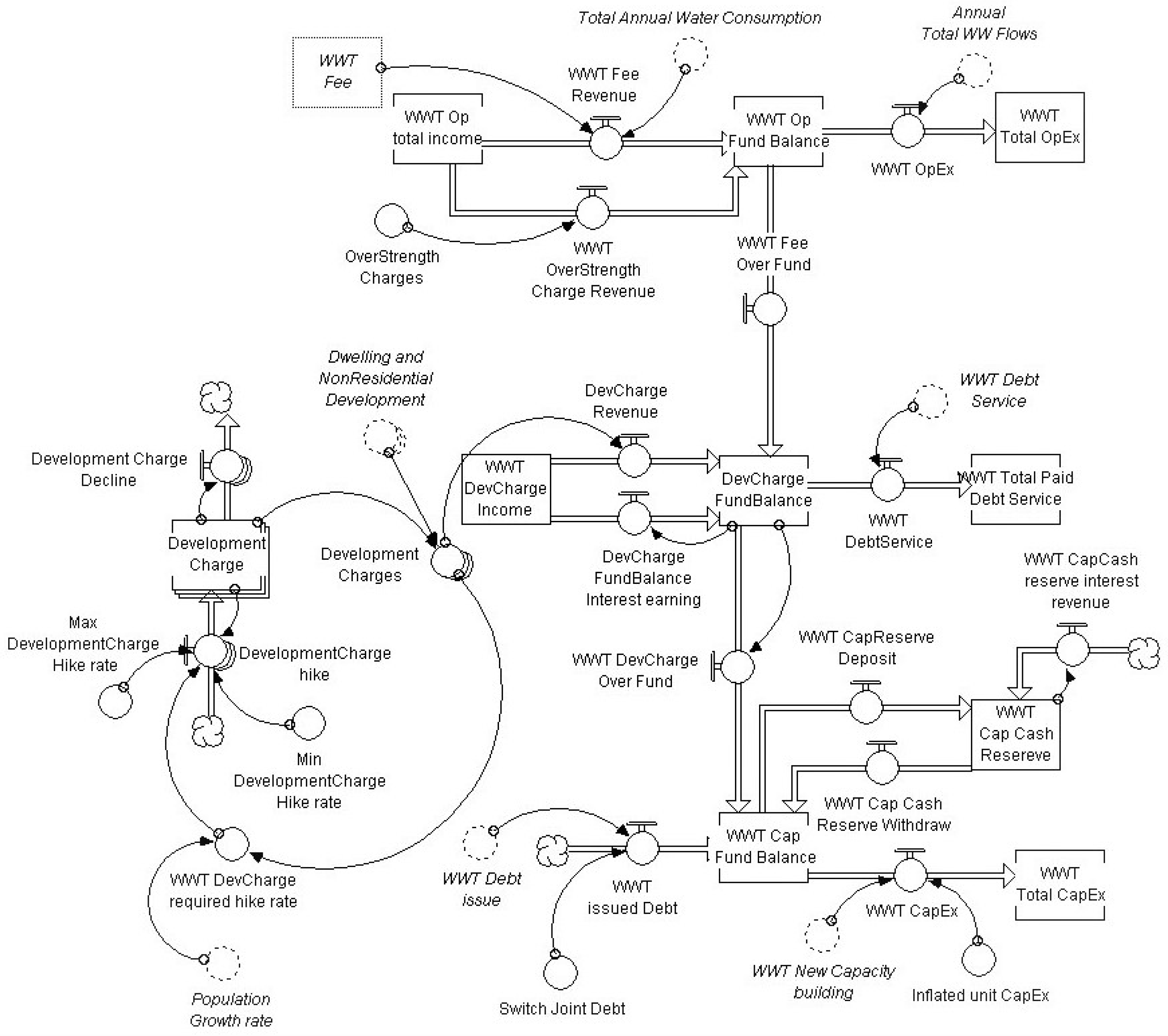
WWTP Finance Model

A new module is developed for the WWTPs finance sector. Similar to the WWC finance structure, surplus revenues are available to lower the fund-balance stocks presented in Figure 11.
The revenues are generated from collecting the user-fees (WWT_Fee [$/m3]) and OverStrength_Charges [$/year] and are primarily paid towards the operational expenses (WWT_OpEx [$/year]). Development_Charges [$/unit and $/m2] are allocated to recover the cost of developing new urban area and are governed by the Province of Ontario under Development Charge Act [35]. If the utility has debt, the revenues from development charges are first allocated to pay debt services (WWT_DebtService [$/year]), and the surplus becomes available for paying the capital expenses (WWT_CapEx [$/year]).
The total development charge (DC) is the sum of the residential and non-residential development charges, which are calculated using Equation (3) and (4), respectively
DCresidential (t) = Nresidential × [(1 − UDI) × S(t) + (UDI × A(t))]
where
  • t [year] is the current time;
  • DCresidential (t) [$/year] represents the revenue of issuing permits for residential building constructions in year t;
  • Nresidential [household/year] is the number of households added to the current population in year t;
  • UDI [%] represents the urban densification index;
  • S(t) [$] is the development-charge for single and attached houses in year t;
  • A(t) [$] is the development-charge for apartments and lodging units in year t.
DCnon-residential (t) = ADnon-residential × [(1 − UDI) × NR (t)]
where
  • t [year] is the current time;
  • DCnon-residential (t) [$/year] represents the revenue of issuing permits for construction of non-residential buildings in year t;
  • ADnon-residential [m2/year] is the new area permitted for building commercial, institutional or industrial buildings in year t;
  • UDI [%] represents the urban densification index;
  • NR (t) [$/m2] is the development-charge for non-residential area development in year t.
When UDI = 0%, the model will simulate the no urban densification scenario, in other words, non-residential area is developed at the same rate as the population growth rate, and only single houses and townhouses will be built to accommodate new population. In contrast, when the UDI = 100%, the model assumes that only apartments and lodging units will be built. The most probable policy would be a 50% urban densification.
If the cash-reserve scenario is selected, the surplus cash will be reserved to up to 50% of the replacement value of WWTPs in reserve (WWT_CapCash_Reserve [$/year]) for paying future capital expenses. If the revenues into capital fund balance (WWT_Cap_FundBalance [$]) are insufficient to pay for the capital-work expenses, the utility has the option to issue debt to maintain a zero-fund balance.

3.2.4. Environment Sector

Greenhouse gas (GHG) emissions are calculated and used as a proxy indicator for the environmental sustainability assessment. The following sections describe the GHG calculation model implemented into the SD Model.

GHG Calculation Model

The GHG module is developed to capture the variations and dynamics in GHG emissions as the results of different asset management scenarios. The annual total GHG emission is comprised of the following variables, which are described in the next subsections.
Annual GHG emission from WWT processes;
Annual GHG emission from electric energy-use;
Annual GHG emission from ICG5 pipes’ replacement, new pipes’ installations, and ICG4 pipes’ rehabilitation.

GHG Emission from WWT Processes:

Three sources of GHG emissions are attributed to the treatment processes: CO2, CH4, and N2O gas emissions. The CO2 gas emission is classified as “biogenic” emission—since it would otherwise br emitted trough natural process of decay—and is not accounted in most referred to protocols such as the Intergovernmental Panel on Climate Change (IPCC) [36].
The annual methane gas CH4 and nitrous oxide N2O emissions are estimated based on the IPCC protocol [36]. Annual methane gas emission is calculated using Equation (5) as
CH4 (t) = ∑(Ui × Tij × EFj) × (IBOD (t) − SBOD (t)) − R
where
  • t [year] is the current time;
  • CH4 (t) [kg/year] represents the mass of methane gas emissions in year t;
  • Ui [%] represent the fraction of population in income group i as rural, urban high income, and urban low income;
  • Tij [%] indicates the treatment pathway j as centralized well managed aerobic treatment, overloaded aerobic treatment, anaerobic digester, etc., served for each group of people in different income groups or (i);
  • EFj [kg/year] is the emission factor in each treatment pathway;
  • IBOD(t) [mg/l] is the BOD concentration of wastewater inflow at WWTP in year t;
  • SBOD(t) [mg/l] is the BOD in removed sludge from WWTP in year t;
  • R [kg CH4 /year] represents the recovered methane gas from WWTP in each studied year.
In IPCC manual [36], 95% of Canadians are classified as high-income people, and the most common WWT method are centralized aerobic WWT and lagoons for both domestic and industrial wastewater. In Ontario, almost the entire population is connected to centralized treatment systems, where secondary-mechanical treatment are applied to remove most of organic matters [37].
Based on the IPCC manual [36], the methane gas emission factor for well managed aerobic treatment systems is considered to be zero. The methane gas emission can be negative if the biogas from anaerobic treatment of wastewater sludge is used for heat and energy recovery.
The annual N2O emission is calculated using Equation (6) as
N2O (t) = P (t) × 0.004
where
  • t [year] is the current time;
  • N2O (t) [kg/year] represents the mass of nitrous oxide emissions in year t;
  • P (t) [capita] is the population in year t;
  • 0.004 [kg/capita/year] is the mass of nitrous oxide emission per person per year (industrial and commercial discharges are also attributed to the residential users).
Therefore, the total annual GHG emissions from the WWT processes is calculated by Equation (7) as
GHG (t) = 23 × CH4 (t) + 296 × N2O
where
  • t [year] is the current time;
  • GHG (t) [kg/year] represents the equivalent mass of CO2 gas emitted from WWT processes in year t;
  • 23 [kg CO2/kg CH4] represents the relative global warming potential of CH4 gas compared to an equivalent mass of CO2 gas;
  • CH4 (t) [kg/year] is the annual CH4 emission calculated in Equation (5);
  • 296 [kg CO2/kg N2O] represents the relative global warming potential of N2O gas compared to an equivalent mass of CO2 gas;
  • N2O [kg/year] is the annual N2O emission calculated in Equation (6).

GHG Emission from Electric Energy Use:

From a life-cycle perspective, energy-use accounting should be done for all life-cycle stages of a studied product or service, including the manufacturing of materials, construction of structures, operation and maintenance of wastewater-collection, and rehabilitation and renewal of infrastructure parts, as well as the disposal of waste materials and end-of-life components.
Based on a study done by the United State Environmental Protection Agency [38], more than 95% of energy-use is attributed to the operational and maintenance stages of water and wastewater systems. Therefore, the energy footprint modeling is centered on the operation, maintenance, and rehabilitation activities. The energy footprints of WWC asset management activities are the sum of all activities listed below:
  • Annual_Energy_use_for_sewage_capital_works [gigajoule/year], which includes the energy used for new pipes installation and ICG4 pipes rehabilitation activities;
  • Annual_Energy_used_for_sewage_collection [gigajoule/year];
  • Annual_Energy_used_for_WWT [gigajoule/year];
  • Annual_energy_used_for_WT [gigajoule/year];
  • Annual_energy_used_for_water_distribution [gigajoule/year];
  • Annual_Energy_use_for_sludge_transportaiton [gigajoule/year] to a central treatment facility such as incineration plant or landfill site;
  • Sludge_treatment_Energy [gigajoule/year] produced or used in sludge treatment processes.
The GHG emission factors are used to convert the energy-use rate to kg CO2 eq. for various energy resources. The GHG emission factor for one kwh electrical energy is calculated based on the energy resources used to generated 1 kwh electricity, which is considered to be 125 g/kwh in Ontario [39].

GHG Emissions from Pipes’ Installation, Replacement, and Rehabilitation:

Rehabilitation activities, particularly when done by open-cut trenching technologies, can lead to traffic delays and consequently more GHG emissions from cars’ engine-fuel combustion [30]. Average GHG emission factors for traffic delays are calculated using the methodology described in [30]. The annual GHG emissions form traffic disturbances can be calculated using Equation (8) as
GHG road system (t) = 2 × ICG4 (t) + 64 × (ICG5 + NSP)
where
  • t [year] is the current time;
  • GHG_raod_ststem (t) [kg/year] represents the equivalent mass of CO2 emitted from traffic disturbances in year t;
  • 2 [kg CO2eq.)/m] represents the GHG emission factor for rehabilitation of ICG4 pipes in year t by using trenchless technologies;
  • ICG4 (t) [m/year] is the length of ICG4 pipes rehabilitated in year t;
  • 64 [kg CO2/m] represents the GHG emission factor for replacement of ICG5 or installation of new WWC pipes using open-cut technology in year t (daily traffic is assumed to be 3500 vehicles/day);
  • ICG5 [m/year] is the length of ICG5 pipes being replaced in year t;
  • NSP [m/year] is the length of new WWC pipes being installed in year t.

4. SD Model Interface

To facilitate the use of the SD model, a user control panel is designed at the user-interface layer of the Stella software. It includes a set of data-entry tables and keys for adjusting several policy levers used for developing scenarios. It also includes graphs and tables that shows the sustainability performance of the WWC and WWTP systems. Each component is described in this section.

4.1. Initial Data Entries

Several data-entry tables that specify the initial data required in each sector before asset management scenarios are run provided at the user-interface layer of the SD model. Initial data related to the natural environment, physical infrastructure, consumer, and finance sectors are presented in Table 1, Table 2, Table 3 and Table 4, respectively.

4.2. Policy Levers

To facilitate applying the SD model and defining various scenarios, a series of policy are provided in the user-interface layer. Table 5 presents the policy levers provided in the user-interface layer.
Three policy levers introduced by Rehan et al. [19] are adopted for the physical sector to test various asset management strategies for WWC systems. The “Preferred rehabilitation rate” [%] policy lever defines the maximum rehabilitation rate of WWC pipes. The annual rate of WWC pipes’ rehabilitation is constrained by the capital fund balance and the length of ICG5 pipes in each year.
The “Max acceptable ICG5 fraction” [%] policy lever is used to define the percentage of network that can acceptably be in the worst condition grade. This value reflects the maximum tolerance of service users and the operational capacity of the studied utility to deal with ICG5 pipes failures, and can be adjusted to any value from 0% to 100%. If the fraction of pipes in the worst condition grade exceeds the “Max acceptable ICG5 fraction” [%], the model will adjust to a new rehabilitation rate above the preferred rehabilitation rate, to reduce their fraction to the acceptable level within the limited number of years specified by the “ICG5 elimination period” [year] policy lever. In that period, the WWC utility should generate enough revenue to support sufficient capital expenses for reducing the ICG5 percentage to below the acceptable level.
The “Rehab ICG4” switch provides the option to include rehabilitation of ICG4 pipes in the asset management plan. If the “Rehab ICG4” switch is on, the capital fund remaining, after spending on ICG5 replacement and WWC pipe installation for network expansion, will be allocated for rehabilitation of the ICG4 pipes.
Seven finance policy levers are developed for the WWC and WWT finance sectors. The “WWC allowable fee-hike rate” [%] and “WWT max allowable fee-hike rate” [%] are used to constrain the annual WWC and WWT fee increases, respectively. As discussed in Section 3.1, the WWC and WWT fees are increased/decreased in response to the additional/reduction of operational expenses for the WWC and WWT systems, and form the (R1) and (R2) reinforcing loops, respectively.
When the “Sewage treatment fee decline” switch is turned on, the WWT fee will rise or fall according to the changes in annual operational expenses. When the switch is turned off, the WWT fee hike will be constrained by the minimum fee hike rate specified by the “WWT min allowable fee-hike rate” [%] policy lever. This allows the WWT-fee based revenue to exceed the current operational expenses and transfer surplus cash to the development charge fund-balance to spend on capital expense. The development-charge hike rates are always constrained by a minimum hike rate specified by the “WWT min development-charge hike rate” [%] policy lever. The minimum hike rates can receive any value between 0% and the “WWT max development-charge hike rate” [%].
The “WWC desired capital-reserve fraction” [%] and “WWT desired capital-reserve fraction” [%] policy levers are set similar to the Rehan at al. [20] and Ganjidoost et al. [23] models. The maximum reserve capacity for the WWC and WWTP finance sectors are defined based on 4% replacement value of the WWC and 100% replacement value of the WWTP asset, respectively.
It is important to note that the minimum fee-hike rate policy lever leads to reserve cash in opposite circumstances than the cash reserving policy lever. By applying the cash reserving policy lever, the advanced SD model will adjust the WWT fee up to the maximum fee-hike rate. Thus, starting cash reserving, as soon as possible, to meet the defined reserve capacity. However, by applying the minimum-fee hike rate policy lever, the model will adjust the WWT fee to the minimum fee-hike rate, thus commencing cash reserving only during the years when the WWT fees require no increase to pay operational expenses.
The “Population growth rate” [%] and “Urban densification rate” [%] are the two policy levers employed to formulate future scenarios related to the consumer sector, both of which can receive any value from 0%–100%. A 0% urban densification scenario will cause the WWC pipe network length to grow at the same rate as the population growth rate, which incurs capital and operational expenses for the WWC system. In contrast, in a 100% urban densification scenario, new population is served within the current WWC pipe network, which avoids the installation and operation of new pipes.

4.3. Advanced SD Model Outputs

The impact of strategic decisions on the asset management of wastewater infrastructure systems can be monitored at the user-interface layer of the Stella software. Some of the key output variables that represent the WWC and WWTP system dynamic behaviors over the simulation period are presented in Table 6.
Several studies discussed the selection of quantitative and qualitative indicators for sustainability assessment of water and wastewater systems. Balkema et al. [40] reviewed and categorized the available sustainability assessment indicator into four general themes of technical, socio-cultural, economic, and environmental. They argued that multi-objective indicators can be normalized to their maximum or minimum values, and summed together to trade-off between conflicting objectives in the decision-making process. Sahely et al. [41] discussed the interconnections and feedbacks between the variables and further defined sub-criteria such as resource use, emissions, and water quality for environmental sustainability, and, resilience, vulnerability and reliability for engineering sustainability. Recently Ganjidoost et al. [23] proposed a set of time-integrated indicators that are categorized to the infrastructure, sociopolitical, and financial performance indicators, and normalized them to the population and pipe-network length for benchmarking different water and wastewater utilities’ performance.

5. Conclusions

This study does not intend to propose an exhaustive list of sustainability indicators, but, rather, to discuss the utility of the SD model in projecting the sustainability outcomes of strategic decisions for urban water assets and present some of the indicators that are developed in the presented SD model. Some of the output variables are matched with the developed policy levers, for example, the “ICG5-Fraction” or “WWC_Fee” results, which are coupled with the “Max acceptable ICG5 fraction” and “WWC allowable fee-hike rate”. They enable the model users to review and adjust the policy levers for achieving a desirable state. Some others are selected to present the sustainability indicators, such as the “Total_GHG” emission or “Bill-Burden”.
This study makes four unique contributions:
(1).
It extends the system boundary of developed SD models for municipal wastewater infrastructure systems, presented by Rehan et al. [20] and Ganjidoost, A. [22], to include the socio-economic feedback from WWTP systems.
(2).
It advances the scope of the SD models presented in [20,22], to include the environmental consequences of strategic decisions related to asset management planning of wastewater infrastructure system. Additionally, new policy levers, such as population growth and urban densification in the social sector, and minimum fee-hike rates in the finance sector, are employed to enhance the representation of real-world conditions in the asset management planning process.
(3).
The newly developed CLDs will help decision makers to better understand the interrelated behavior of social, environmental, and economic systems, so they can see the whole picture and communicate the issues more effectively to other stakeholders.
(4).
The present SD model is developed as part of the asset management planning framework shown in Figure 1. Application of this model will allow the asset management planners to project the performance of WWC assets onto their future life-cycle, assess the sustainability of strategic asset management decisions, and find synergistic savings and opportunities when planning for the sustainability of these assets.

Author Contributions

Conceptualization, H.M., M.A.K. and A.A.J.U.; methodology, H.M., M.A.K. and A.A.J.U.; software, M.A.K.; validation, H.M., M.A.K. and A.A.J.U.; formal analysis, H.M.; writing—original draft preparation, H.M.; writing—review and editing, H.M., M.A.K. and A.A.J.U.; supervision, M.A.K. and A.A.J.U.; funding acquisition, M.A.K. and A.A.J.U.

Funding

This research was funded by Natural Science and Engineering Research Council of Canada (NSERC) and the Centre for Advancement of Trenchless Technology (CATT) located at the University of Waterloo.

Acknowledgments

We gratefully acknowledge the financial support provided by the NSERC and CATT.

Conflicts of Interest

The authors declare no conflicts of interest. The funders had no role in the design of the study; in the collection, analyses, or interpretation of data; in the writing of the manuscript, or in the decision to publish the results.

References

  1. Government of Canada. Federal Sustainable Development Act; Government of Canada: Ottawa, ON, Canada, 2008.
  2. Government of Canada. Federal Sustainable Development Strategy. Available online: http://fsds-sfdd.ca/index.html#/en/goals/ (accessed on 7 May 2018).
  3. (CSCE) CSCE’s Vision 2020. Available online: https://csce.ca/wp-content/uploads/2018/08/Vision-2020-member-information-August-10-12-jak2.pdf (accessed on 10 May 2019).
  4. Federation of Canadian Municipalities. How to Develop an Asset Management Policy, Strategy and Governance Framework: Set Up A Consistent Approach to Asset Management in Your Municipality; Federation of Canadian Municipalities: Ottawa, ON, Canada, 2018. [Google Scholar]
  5. Federation of Canadian Municipalities. Leadership in Asset Management Program. Available online: https://fcm.ca/home/programs/green-municipal-fund/resources-and-programs/leadership-in-asset-management-program.htm (accessed on 7 May 2018).
  6. FCM. Municipalities for Climate Innovation Program (MCIP). Available online: https://fcm.ca/home/programs/municipalities-for-climate-innovation-program/municipalities-for-climate-innovation-program.htm (accessed on 25 May 2018).
  7. Felio, G.; Lounis, Z. Model Framework for Assessment of State, Performance, and Management of Canada’s Core Public Infrastructure; NRC: Washington, DC, USA, 2009. [Google Scholar]
  8. ISO 55000. Assessments and Road mapping Services. Available online: https://www.assetmanagementstandards.com/assessments-roadmapping/ (accessed on 23 February 2018).
  9. Halfawy, M.M.R.; Newton, L.A.; Vanier, D.J. Review of Commercial Municipal Infrastructure Asset Management Systems. Electron. J. Inf. Technol. Constr. 2006, 11, 211–224. [Google Scholar]
  10. Sala, S.; Ciuffo, B.; Nijkamp, P. A Meta-Framework for Sustainability Assessment Research Memorandum; VU University: Amsterdam, The Netherlands, 2013. [Google Scholar]
  11. Upadhyaya, J.K. A Sustainability Assessment Framework for Infrastructure: Application in Stormwater Systems. Ph.D. Thesis, University of Windsor, Windsor, ON, Canada, 2013. [Google Scholar]
  12. Mohammadifardi, H.; Knight, M.A.; Unger, A.J.A. Development of an asset management planning tool for integrated wastewater collection and treatment systems. In Proceedings of the 36th International Conference of the System Dynamics Society, Reykjavík, Iceland, 7–9 August 2018; pp. 2150–2178. [Google Scholar]
  13. Mirchi, A.; Madani, K.; Watkins, D.; Ahmad, S. Synthesis of System Dynamics Tools for Holistic Conceptualization of Water Resources Problems. Water Resour. Manag. 2012, 26, 2421–2442. [Google Scholar] [CrossRef]
  14. Chung, G.; Lansey, K.; Blowers, P.; Brooks, P.; Ela, W.; Stewart, S.; Wilson, P. A general water supply planning model: Evaluation of decentralized treatment. Environ. Model. Softw. 2008, 23, 893–905. [Google Scholar] [CrossRef]
  15. Biachia, C.; Montemaggiore, G.B. A system dynamics-based simulation experiment for testing mental model and performance effects of using the balanced scorecard. Syst. Dyn. Rev. 2008, 24, 175–213. [Google Scholar]
  16. Das, B.K.; Bandyopadhyay, M.; Mohapatra, P.K.J. System Dynamics Modeling of Biological Reactors for Waste Water Treatment. J. Environ. Syst. 1996, 25, 213–240. [Google Scholar] [CrossRef]
  17. Gillot, S.; De Clercq, B.; Defour, F.; Gernaey, K.; Vanrolleghem, P.; Jeppsonn, U.; Carstensen, J.; Carlsson, B.; Olsson, G. Optimization of Wastewater Treatment Plant Design and Operation Using Simulation and Cost Analysis. In Proceedings of the WEF Conference and Exposition, New Orleans, LA, USA, 9–13 October 1999; pp. 9–13. [Google Scholar]
  18. Parkinson, J.; Schütze, M.; Butler, D. Modelling the Impacts of Domestic Water Conservation on the Sustain Ability of the Urban Sewerage System. Water Environment J. 2005, 19, 49–56. [Google Scholar] [CrossRef]
  19. Rehan, R. Sustainable Municipal Water and Wastewater Management Using System Dynamics. Ph.D. Thesis, University of Waterloo, Waterloo, ON, Canada, 2011. [Google Scholar]
  20. Rehan, R.; Knight, M.A.; Haas, C.T.; Unger, A.J.A. Application of system dynamics for developing financially self-sustaining management policies for water and wastewater systems. Water Res. 2011, 45, 4737–4750. [Google Scholar] [CrossRef] [PubMed]
  21. Rehan, R.; Knight, M.A.; Unger, A.J.A.; Haas, C.T. Development of a system dynamics model for financially sustainable management of municipal watermain networks. Water Res. 2013, 47, 7184–7205. [Google Scholar] [CrossRef] [PubMed]
  22. Ganjidoost, A. Performance Modeling and Simulation for Water Distribution and Wastewater Collection Networks; University of Waterloo: Waterloo, ON, Canada, 2016. [Google Scholar]
  23. Ganjidoost, A.; Knight, M.A.; Unger, A.J.A.; Haas, C.T. Benchmark performance indicators for utility water and wastewater pipelines infrastructure. J. Water Resour. Plan. Manag. 2018, 144. [Google Scholar] [CrossRef]
  24. Rehan, R.; Unger, A.J.A.; Knight, M.A.; Haas, C.T. Strategic Water Utility Management and Financial Planning Using a New System Dynamics Tool. J. Am. Water Works Assoc. 2015, 107, 22–36. [Google Scholar] [CrossRef]
  25. Ganjidoost, A.; Haas, C.; Knight, M.; Unger, A. A System Dynamics Model for Integrated Water Infrastructure Asset Management. In Proceedings of the 33rd International Conference of the System Dynamics Society, Cambridge, MA, USA, 19–23 July 2015; pp. 1–16. [Google Scholar]
  26. Rehan, R.; Knight, M.A.; Unger, A.J.A.; Haas, C.T. Financially sustainable management strategies for urban wastewater collection infrastructure—Development of a system dynamics model. Tunn. Undergr. Space Technol. 2014, 39, 116–129. [Google Scholar] [CrossRef]
  27. Min, K.; Yeats, S.A. Water Conservation Efforts Changing Future Wastewater Treatment Facility Needs. Flourida Water Resour. J. 2011, 39–41. Available online: https://fwrj.com/techarticles/0811%20tech2.pdf (accessed on 10 May 2019).
  28. DeZellar, J.T.; Walter, J.M. Effects of Water Conservation on Sanitary Sewers and Wastewater Treatment Plants. Water Pollut. Control Fed. 1980, 52, 76–88. [Google Scholar]
  29. Marleni, N.; Gray, S.; Sharma, A.; Burn, S.; Muttil, N. Impact of water management practice scenarios on wastewater flow and contaminant concentration. J. Environ. Manag. 2015, 151, 461–471. [Google Scholar] [CrossRef] [PubMed]
  30. Rehan, R.; Knight, M.A. Do Trenchless Pipeline Construction Methods Reduce Greenhouse Gas Emissions; Centre for the Advancement of Trenchless Technologies (CATT) Department of Civil and Environmental Engineering, University of Waterloo: Waterloo, ON, Canada, 2007; p. 19. [Google Scholar]
  31. Richmond, B. An Introduction to Systems Thinking; Isee Systems, Inc.: Lebanon, NH, USA, 1997; ISBN 0970492111. [Google Scholar]
  32. WRc Sewerage Rehabilitation Manual; Water Research Centre: Swindon, UK, 2011.
  33. Recommended Standards for Wastewater Facilities; Health Research, Inc., Health Education Services Division: Albany, NY, USA, 2014.
  34. Statistics Canada Non-residential Building Construction Price Index, Fourth Quarter 2016. Available online: https://www150.statcan.gc.ca/n1/daily-quotidien/170214/dq170214a-eng.htm (accessed on 31 October 2018).
  35. Development Charges Act. Available online: https://www.ontario.ca/laws/statute/97d27 (accessed on 10 May 2019).
  36. Doorn, M.R.J.; Towprayoon, S.; Manso Vieira, S.M.; Irving, W.; Palmer, C.; Pipatti, R.; Wang, C. Chapter 6 Wastewater Treatment and Discharge. In Intergovernmental Panel on Climate Change (IPCC) Guidelines for National Greenhouse Gas Inventories; Institute for Global Environmental Strategies (IGES): Hayama, Japan, 2006; Volume 5. [Google Scholar]
  37. Environment Canada. 2011 Municipal Water Use Report; Environment Canada: Gatineau, QC, Canada, 2011. Available online: https://www.ec.gc.ca/doc/publications/eau-water/COM1454/survey8-eng.htm (accessed on 10 May 2019).
  38. Cashman, S.; Gaglione, A.; Mosley, J.; Weiss, L.; Hawkins, T.R.; Ashbolt, N.J.; Cashdollar, J.; Xue, X.; Ma, C.; Arden, S. Environmental and Cost Life Cycle Assessment of Disinfection Options for Municipal Wastewater Treatment; National Homeland Security Research Center: Cincinnati, OH, USA, 2014; ISBN 9781583219003.
  39. Sahely, H.R.; MacLean, H.L.; Monteith, H.D.; Bagley, D.M. Comparison of on-site and upstream greenhouse gas emissions from Canadian municipal wastewater treatment facilities. J. Environ. Eng. Sci. 2006, 5, 405–415. [Google Scholar] [CrossRef]
  40. Balkema, A.J.; Preisig, H.A.; Otterpohl, R.; Lambert, F.J.D. Indicators for the sustainability assessment of wastewater treatment systems. Urban Water 2002, 4, 153–161. [Google Scholar] [CrossRef]
  41. Sahely, H.R.; Kennedy, C.A.; Adams, B.J. Developing sustainability criteria for urban infrastructure systems. Can. J. Civ. Eng. 2005, 32, 72–85. [Google Scholar] [CrossRef]
Figure 1. Application of the proposed sustainability assessment tool in the ISO 55000 [8] asset management framework.
Systems 07 00026 g001
Figure 2. A complete water and wastewater infrastructure system.
Systems 07 00026 g002
Figure 3. Causal loop diagram (CLD) for WWC systems.
Systems 07 00026 g003
Figure 4. CLD for WWTP systems.
Systems 07 00026 g004
Figure 5. CLD for integrated WWC and WWTP systems.
Systems 07 00026 g005
Figure 6. Impact of population and urban densification.
Systems 07 00026 g006
Figure 7. Completed CLD of WWTP and WWC physical, finance, social, and environmental sectors.
Systems 07 00026 g007
Figure 8. The WWC pipe network model.
Systems 07 00026 g008
Figure 9. WWTP capacity model.
Systems 07 00026 g009
Figure 10. WWC finance model.
Systems 07 00026 g010
Figure 11. WWT finance model.
Systems 07 00026 g011
Table 1. Data entry for environment sector.
Data EntryUnitPractical Range
Life-cycle energy used for pipes manufacturingMJ/kg50–100
Life-cycle energy used for new pipe installationMJ/m1000–2000
Life-cycle energy use for drinking water treatmentMJ/m30–3
Energy use for water distribution (WD)MJ/m30–3
Energy use for wastewater collection (WWC)MJ/m30–1
Life-cycle energy used for wastewater treatmentMJ/m30–3
Life-cycle energy used for treatment plant constructionMJ/m30–1
Life-cycle energy used for pipes manufacturingMJ/kg50–100
Table 2. Data entry for physical infrastructure sector.
Data EntryUnitPractical Range
Initial length of pipes based on material and internal condition gradeKm0–103
Initial number of water meters based on pipe diameter-0–105
Initial capacity of wastewater treatment plants (WWTPs) m3/day0–1010
Initial total infiltration and inflow m3/year0–1010
Initial equivalent suspended solid generation kg/year/capita40–70
Initial equivalent biological oxygen demand (BOD) generation kg/year/capita50–70
Table 3. Data entry for consumer sector.
Data EntryUnitPractical Range
Initial populationcapita0–5 × 10⁹
Average household sizecapita2–4
Population growth ratepercent/year0–100
Initial water demand for residential users liter/day/capita150–300
Minimum water demand for residential usersliter/day/capita100–150
Initial water demand for non-residential usersliter/year0–5 × 1018
Bill hardship threshold% of household income0.1–100
Initial number of residential apartment and lodging -10–5 × 10⁵
Initial number of houses and townhouses-10–5 × 10⁵
Initial non-residential area m210–5 × 10⁷
Initial WWC fee for residential user$/m30.01–10
Initial WWC fee for non-residential user$/m30.01–10
Initial WWT-free residential user$/m30.01–10
Initial WWT-free non-residential user$/m30.01–10
Table 4. Data entry for finance sector.
Data EntryUnitPractical Range
Price elasticity of water demand for residential users-0–1
Average household income $/year50,000–90,000
Initial WWC cost $/m30.1–10
Initial WWT cost $/m30.1–10
Initial debt/reserve of utility (for WWC model)$0–109
Initial debt/reserve of region (for WWTP model)$0–109
Annual revenues from industries for over strength wastewater discharge $/year0–109
Unit maintenance cost of WWC pipes in each ICG class$/m/year2–10
Unit development charge for apartments/lodges $/unit1000–3000
Unit development charge for houses/townhouses$/unit2000–5 × 104
Unit development charges for non-residential areas$/m20.1–10
Initial service charges based on water meter sizes$/m200–2000
Unit cost of CIG4 pipes’ rehabilitation $/m400–600
Unit cost of ICG5 pipes replacement $/m700–1000
Inflation rate for electrical energy cost-0–5
Inflation rate for non-residential building construction cost-0–7
Fixed borrowing rate -0–7
Fixed saving rate -0–5
Price elasticity of water demand for residential users-0–1
Table 5. Policy levers at the interface layer.
Policy LeverUnitRange or Value
Physical sector
Preferred rehabilitation rate%0–100
Max acceptable ICG5 fraction%0–100
ICG5 elimination periodyear0–100
Rehab ICG4 switch-0 or 1
Finance sector
WWC allowable fee-hike rate%0–100
WWT max allowable fee-hike rate%0–100
WWT min allowable fee-hike rate%0–(WWT max allowable fee hike rate)
Sewage treatment-fee decline switch-0 or 1
WWT max development-charge hike rate%0–100
WWT min development-charge hike rate%0–(WWT max development-charge hike rate)
WWC desired capital-reserve fraction%0–4
WWT desired capital-reserve fraction%0–100
Consumer sector
Population growth rate%0–100
Urban densification rate%0–100
Table 6. List of output variables plotted in the user-interface layer of the SD model.
VariablesUnitDescription
Physical sector
Actual_Rehab_Rate (t)%Fraction of WWC pipe network that has been replaced or rehabilitated in year t
ICG5_Fraction (t)%Fraction of ICG5 pipes length that is in service within the WWC pipe network in year t
Avg_ICG_Network(t)ICGAverage internal condition grade of the network in year t
Network_Expns(t)mLength of WWC pipe network expanded in year t
Generated_WW_Res (t)m3/daySewage generated by residential users in year t
Generated_WW_Non-Res (t)m3/dayWastewater generated by non-residential users in year t
I&I(t)m3/dayInflow and infiltration volume in year t
Environment sector
Energy_FootprintgigajoulesTotal energy used in WWC and WWTP systems in year t
Total_GHGtone CO2Total direct and indirect GHG emissions in year t
Finance sector
WWC_Fee (t)$WWC fee hike rate for residential users in year t
WWT_Fee (t)$WWT fee hike rate for residential users in year t
DevCharge_Res_Apt(t)$Development charges for building new residential apartments in year t
DevCharge_Res_House(t)$Development charges for building new residential houses in year t
DevCharge_NonRes(t)$Development charges for development of non-residential areas in year t
WWC_Op_FB(t)$Operational fund balance of WWC system in year t
WWC_Cap_FB(t)$Capital fund balance of WWC system in year t
WWT_Op_FB(t)$Operational fund balance of WWT system in year t
WWT_CevCharge_FB(t)$Development charge fund balance of WWT system in year t
WWT_Cap_FB(t)$Capital fund balance of WWT system in year t
WWC_Debt(t)$Amount of issued debt for capital work expenses for WWC pipe network system in year t
WWT_Debt(t)$Amount of issued debt for capital work expenses for WWTP capacity upgrading in year t
OpEx_WWC(t)$Operational and maintenance expenses of WWC system in year t
CapEx_WWC(t)$Capital expenses of WWC system in year t
OpEx_WWT(t)$Operational and maintenance expenses of WWT system in year t
CapEx_WWT(t)$Capital expenses of WWT system in year t
Reserve_WWT_Cap%Fraction of extra capacity in WWTP system in year t
Consumer sector
Water_demand_Resl/c/dAverage daily water demand of residential users in year t
Bill_Burden%Fraction of an average household income which should be paid for WWC and WWT services

