Towards a Dynamic Equilibrium-Seeking Model of a Closed Economy


MEResearch, Level 5, 507 Lake Rd, Takapuna, Auckland 0622, New Zealand
*
Author to whom correspondence should be addressed.
Systems 2020, 8(4), 42; https://0-doi-org.brum.beds.ac.uk/10.3390/systems8040042
Submission received: 17 September 2020
/
Revised: 27 October 2020
/
Accepted: 29 October 2020
/
Published: 4 November 2020
(This article belongs to the Section Systems Practice in Social Science)
Abstract
:Economics has long been concerned with the development of tools to help understand and describe the interactions among economic actors including the circular flow of economic resources. This paper expands our available toolkit of models, by describing a novel dynamic equilibrium-seeking model of a closed economy. The model retains many of the key features of state-of-the-art Computable General Equilibrium (CGE) models including economic interdependence, input substitution, nested production functions, and so on. A distinguishing feature of this model is that it adopts price-related balancing feedback loops that simulate the self-regulating behaviour of a dynamic economic system. Our modelling shows not only equilibrium states (as per conventional CGE models), but the transition path toward an often-changing equilibrium. This facilitates the investigation of out-of-equilibrium dynamics and behaviour adaptation typical of largescale disruption events.
1. Introduction
We often use models as a tool to analyse and visualise the change in systems. They simplify complex systems, enabling us to better understand and explain structure and behaviour, often with the aim of informing decision making [1,2]. Models can vary greatly in nature and scope, ranging from conceptual models that qualitatively highlight important connections in real-world systems, through to highly sophisticated computer models, where complex mathematical relationships transform sets of user-defined inputs into a simulated set of indicators of key system processes over space and time. In this paper, we explicitly focus on the assessment of economic system consequences using whole-of-economy modelling.
For whole-of-economy multi-regional analysis, Computable General Equilibrium (CGE) models have over the last couple of decades become a popular modelling approach among economists [3,4,5,6]. Of course, no model is perfect, and the selection of the most appropriate modelling approach must be guided by the system being analysed and the aims of the modelling exercise. The ability of CGE models to incorporate price responses within production and consumption behaviours, and to trace the circular flow of income through economic systems, are features often identified as attractive for policy-oriented economic applications. When transition pathways or significant system changes are an important aspect of the application under enquiry, the structure of a CGE model is less suitable in providing useful insights.
In this paper, a novel dynamic equilibrium-seeking (DES) model of a closed (i.e., excluding trade) economy is developed. Like many CGE models, a core feature of the DES model is the importance of interrelations or interdependence among the different parts of an economy. Other distinguishing features of CGE models are also incorporated within this DES model. Economic resources (commodities, factors), for example, are represented by both prices and quantities, and nested production functions (of a Constant Elasticity of Substitution (CES) form) allow for substitution of inputs in response to changes in relative prices. Unlike most CGE models, however, the DES model is formulated not as an optimisation or mathematical programming problem, but rather using finite difference equations in the form of a System Dynamics model. The DES is uniquely able to trace (1) multiscale transition pathways, (2) account for out-of-equilibrium dynamics that are often typically of sudden unforeseen disruption events (e.g., natural hazards, pandemics, terrorism attacks, financial crises), and (3) more readily integrate with other socio-economic (demographic, land-use change, transportation) and environmental (biogeochemical—resources, energy, climate change, ecosystem service) systems models. The DES model is also scalable to multiple regions with numerous commodities, industries and factors interacting dynamically. Together these features provide for a more holistic evaluation of impacts.
This paper commences with a short introduction to some of the important antecedents to the DES model. The paper then describes the development of the DES model, beginning with an overview of the key dynamics controlling price change. We then develop the model in two stages. Firstly, the DES constant factor (“DES CF”) model is formulated to mimic a simple comparative static CGE model (see [5,6]), but with the inclusion of self-regulating price mechanisms. Given identical initial conditions, it is possible to produce results from the DES CF model that are identical to a comparative static CGE model, but simultaneously depict the transition pathway taken through time to reach this equilibrium. Secondly, we further develop the model by including changes in labour and capital factor stocks and rename it as the DES Factor Growth (“DES FG”) model. Our results investigate the dynamic behaviour of the DES CF and FG models, including an application of an exogenous disruption shock. We, in turn, critique the DES and suggest further extensions. The paper ends with concluding remarks.
Antecedents
An interest in understanding and describing the interactions and interdependencies occurring between various economic actors, and in the notion of a circular flow of economic resources, has long been of interest in economics. The eighteenth-century Physiocrat Francois Quesnay’s Tableau Économique [7] is a founding pillar, providing a diagrammatic representation of how expenditures can be traced through an economy in a systematic way. The development of a general equilibrium theory of a competitive market by Léon Walras (1954) is a further critical antecedent [8]. Walras formulated the state of the economic system, in terms of supply and demand for goods/services, as the solution of a system of simultaneous equations by assuming that consumers act to maximise utility, producers act to maximise profits, and perfect market conditions prevail. Wassily Leontief (1941) created Input–Output Analysis by simplifying the Walrasian framework resulting in an “empirical study of interrelations among the different parts of a national economy as revealed through covariations of prices, outputs, investments, and incomes” [9]. Kenneth Arrow and Gérard Debreu [10,11,12,13] further extended Walras’ work by providing formal mathematical proofs of the existence of such equilibrium for a competitive economy. Their work provided fundamental insights into the factors and mechanisms that determine relative prices, resource allocation, and income distribution within and between economies.
Computable General Equilibrium (CGE) models are an attempt to use general equilibrium theory within a numerical framework. The emergence of CGE modelling is generally attributed to Johansen’s [14] pioneering (1960) multi-sectorial study of economic growth, but Harberger’s (1962) analysis of tax policies [15], Scarf’s (1967) and Scarf and Hansen’s (1973) work on conditions for the existence of and algorithms for computation of Walrasian equilibria [16], and rapid advances in computer technology also represented critical development milestones [17]. CGE models are now a standard item in the toolbox of economists concerned with policy-oriented research. By design, CGE models are focused on describing steady states of economic equilibrium, usually following an exogenous policy intervention or economic shock. This has included analysis of major tax reforms (e.g., [18,19,20,21,22]), development issues (e.g., [23]), changes in trade (e.g., [24,25,26,27]), agriculture, energy and environmental policy (e.g., [28,29,30,31]) and assessment of major disruption events (e.g., [32,33,34,35]). It is worth noting most CGE models are made possible by the incorporation of an Input-Output Table [36,37,38]; which provides a database for populating the model’s initial conditions. This is also true of the DES model described in this paper.
Proponents of CGE modelling often point towards the ability of CGE models to incorporate price responses within production and consumption behaviours. The substitution of capital for labour by firms in response to increasing relative labour costs, for example, or changing household consumption choices in response to changes in relative commodity prices. CGE models also tend to place greater emphasis on the flow of income through institutional sectors. Conversely, CGE models are typically based on assumptions of optimising behaviour and market equilibrium. While these assumptions provide useful insights into many kinds of phenomena, circumstances do exist where they are sufficiently restrictive that most common forms of dynamic CGE (including “recursive dynamic” [4] and “perfect foresight” [39] implementations) models are unsuitable for understanding transition pathways between equilibria, particularly when assessing out-of-equilibrium dynamics and emergent behavioural change or adaptation that often occur with major disruptive events. Under both approaches the sequence linking two equilibria is typically unexplained, and the length of time it takes to transition between equilibria, although unknown, is often assumed to be one year.
A modelling approach that is clearly oriented towards the study of system changes over time is System Dynamics [40,41,42,43,44]. At the heart of the System Dynamics approach is the identification of feedback structures within systems. System Dynamics models rely on numerical methods to approximate solutions for ordinary differential equations (using finite difference equations) along a path of successive time-steps. Although these approximations necessarily introduce some questions of accuracy, they are essential in most cases, as the nonlinearity of the equations makes obtaining analytic solutions impractical. Furthermore, it significantly widens the scope of modelling exercises, enabling very complex systems to be represented within a computer simulation model. The graphical user interfaces of most System Dynamics packages are user-friendly enabling end-users to easily grasp model structures, interactively run models and review results.
2. A Dynamic Equilibrium-Seeking Model
Before commencing with a full description of the DES model, it is helpful to set out conventions and notations used and to provide details of how supply, demand and price may be represented in a System Dynamics model, as the behaviours produced by these relationships underpin the equilibrium-seeking nature of the DES model.
2.1. Conventions and Notation
In the equations that follow, “stocks” are represented mathematically by bold font, with the first letter capitalised. Diagrammatically they are represented by a rectangular box. Flows are represented mathematically in a lowercase italicised font and diagrammatically by using a pipe-valve symbol, i.e., ![Systems 08 00042 i001]() . “Exogenous converters” are represented mathematically by capital letters and italics, while all “endogenous converters” are represented by a lowercase italicised font. Converters are used to provide clarity to the modelling process by explicitly showing how flows are calculated. Subscripts are used in equations to indicate the dimensionality of a variable. For example, the stock Industryaccountj denotes an accumulation of financial resources held by each industry j. A full list of stocks, flows and converters applied in the DES model is provided in the Supplementary Material.
. “Exogenous converters” are represented mathematically by capital letters and italics, while all “endogenous converters” are represented by a lowercase italicised font. Converters are used to provide clarity to the modelling process by explicitly showing how flows are calculated. Subscripts are used in equations to indicate the dimensionality of a variable. For example, the stock Industryaccountj denotes an accumulation of financial resources held by each industry j. A full list of stocks, flows and converters applied in the DES model is provided in the Supplementary Material.
 . “Exogenous converters” are represented mathematically by capital letters and italics, while all “endogenous converters” are represented by a lowercase italicised font. Converters are used to provide clarity to the modelling process by explicitly showing how flows are calculated. Subscripts are used in equations to indicate the dimensionality of a variable. For example, the stock Industryaccountj denotes an accumulation of financial resources held by each industry j. A full list of stocks, flows and converters applied in the DES model is provided in the Supplementary Material.
We also chose to use Euler’s method to numerically approximate the solution to the DES model as it can deal with delays. It is also an explicit method, meaning that calculating the value of the stocks at a time step only requires knowledge of the values at the previous time step. The choice of the time step (i.e., Δt) is always a trade-off between numerical accuracy and stability, and computational time. Given that the model in this paper is intended for exposition purposes, a fairly large time step of 0.25 years is selected.
2.2. Representing Supply, Demand and Price in a System Dynamics Model
A central idea put forward in any introductory economics textbook is that in competitive economies, prices enable markets to adjust to a point of equilibrium, where the supply of a good or service is in balance with the demand for that good or service (e.g., [2]). The role of a CGE model is to depict this world numerically for entire economies, where a balance between supply and demand is attained through relationships between price and supply/demand. This, however, presents a relatively static view of demand–supply relationships, providing no information on the processes through which equilibrium is reached.
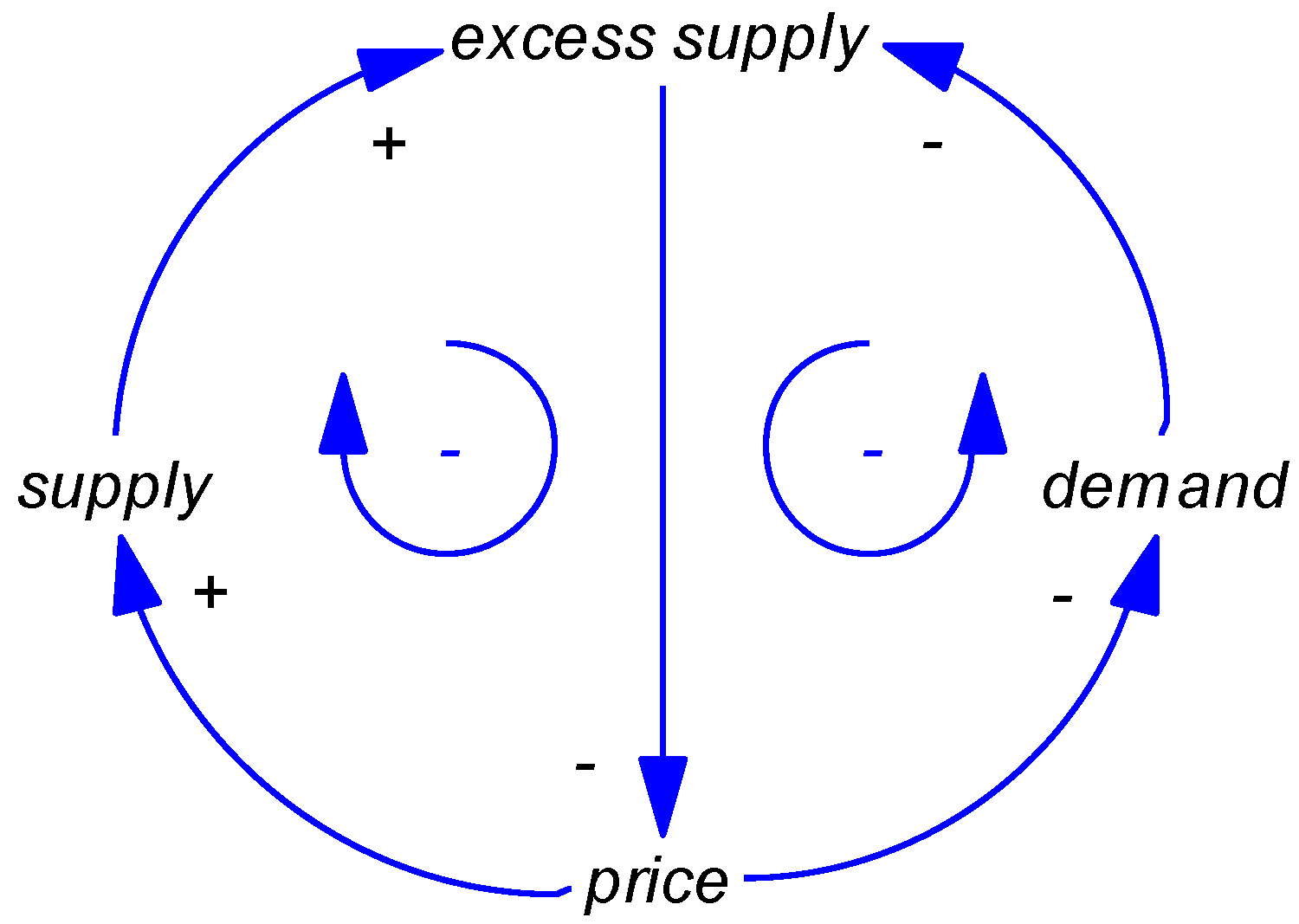
We can depict the relationship between supply, demand and price in a causal loop diagram (Figure 1). An arrow linking two converters indicates a causal association between those converters. A “+” symbol adjacent to the arrow indicates that an increase in the variable at the tail of the arrow causes a corresponding increase in the variable at the head of the arrow, above what it would have been otherwise. Conversely, a “–“ symbol indicates that, compared with a situation with no change, a change in the tail variable causes the head variable to change in the opposite direction.
Imagine that Figure 1 describes the relationship between supply, demand and price for a given commodity. The term “excess supply” denotes a ratio of the level of supply (also termed “production”) relative to the level of demand (also termed “consumption” or “use”). A positive increase in supply will cause excess supply to increase, while the opposite relationship holds between demand and excess supply. Market prices for that commodity are, in turn, influenced by the level of excess supply. When excess supply is less than one (i.e., demand is greater than supply), buyers will increase the price they offer to obtain the quantity that is in short supply. At a higher price, a greater number of producers will be willing and able to supply the subject commodity, hence the positive causal connection between price and supply. Conversely, if excess supply is greater than one, sellers will reduce the price to try to sell the commodity to hard-to-find buyers. The causal connection between price and demand is negative, reflecting the greater ability and willingness of buyers to purchase the commodity at a lower price. For the unique situation when excess demand is equal to one, the market is in equilibrium, and there is no pressure on the price to be adjusted.
There are two types of feedbacks or causal loops created by this relatively simple set of relationships between supply, demand and price. In both cases, the feedback loop is balancing (represented by the two negative symbols at the centre of Figure 1), meaning that a directional change in an initial variable will ultimately cause a change in the opposite direction for that same variable. It is the presence of at least one dominant balancing feedback loop in a system that acts to counter system disturbances or shocks that leads the system ultimately back towards some type of steady-state or goal. As will be seen, the development of an equilibrium-seeking model within System Dynamics is essentially about establishing a number of these price-related balancing feedback loops.
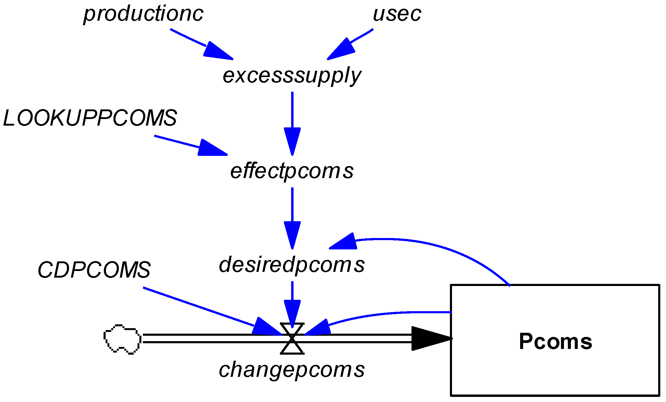
Figure 2 depicts the detail of the price change causal mechanisms shown in Figure 1 as implemented in the DES model using a “stock-and-flow” diagram. The price of commodity i, Pcomsi, is a stock variable and it is defined by the finite-difference equation,
where changepcomsi is the increase in price during the period (∆t). Commodity prices are treated as stocks because markets do not determine these prices instantaneously; rather the process of price adjustment is gradual, with each period building upon the previous.
The greater the relative difference between commodity demand and supply, the greater the relative price change occurring within the model. This mechanism is implemented through Equations (1)–(4). The term LOOKUPPCOMSi in Equation (2) is an exogenous lookup function that determines the relative price change effect, depending on the extent of excess supply. When the excess supply of a commodity excesssupplyi is greater than one, the function returns a value less than one causing price to decrease. The opposite occurs where excesssupplyi is less than one. This formulation of a price change response curve is reasonably generic, most System Dynamics packages provide capabilities to undertaken model calibration (using optimisation procedures) against a known set of historic data. Alternatively, we could reformulate the equation for effectpcomi so that it is determined by a function of form 1/xα, where x is the level of excess supply of commodity i and α is a calibrated parameter. The exogenous price change delay, CDPCOMSi, is a scalar set between 0 and 1. For exposition purposes, we give this scalar a default value of 1.
2.3. The Dynamic Equilibrium-Seeking Model with Constant Factors (DES CF)
Having described the general structure of the price change dynamics, we now provide a full description of the DES model. We begin with a model where it is assumed that there is no change in the economy-wide availability of the factors of production over the simulation period (DES CF).
The model is separated into six modules: Commodities, Industries, Factors, Government, Investment and Savings and Households. Each of these modules is described in detail below. For the sake of brevity, we included only some of the System Dynamics stock-and-flow diagrams for the modules, the remainder are available in the Supplementary Material.
2.3.1. Commodities Module
We begin the description of the Commodities module by noting that it directly incorporates the price change dynamics for commodities already set out in Equations (1)–(4) (see Figure S1 within the Supplementary Material). We added an exogenous industry production tax rate, TAXPRODFj, which creates a wedge between what we can now refer to as the commodity supply price, Pcomsi, and commodity demand price, pcomdi (Equations (5) and (6)).
For simplicity, the model is structured on the basis that each economic activity or industry, denoted by subscript j, produces only one homogenous commodity, thus,
where productionci and productionfj are, respectively, the total production of commodity i output and the total quantity of industry j output. Similarly,
where the converter on the left-hand side denotes the price of industry j output. The Social Accounting Matrix (SAM) data used to populate the initial conditions of the DES model therefore has the same commodity and industry definitions. Modifying the model to allow for joint production is however relatively straightforward.
The quantity of output produced by each industry, productionfj, is determined using composite factors by that industry, compfactoruj, relative to the ratio of composite factor inputs per unit of production, factinputsharej (Equation (7)). Like many CGE models, the DES model employs a Constant Elasticity of Substitution (CES) production function, allowing for substitution between inputs at various industry aggregations or branches within the function. The quantity of composite factors available to industry is thus a combined measure of the labour and capital endowments of that industry (refer to the Factors Module). Most comparative static CGE models assume that there is no substitution between intermediate goods and composite factors, and factinputsharej is therefore set equal to a factor input coefficient AYj, defined by the base year ratio of the quantity of composite factors required, per unit of production by industry j. The DES model, however, allows for the possibility of substitution between intermediate goods and composite factors. Thus, factinputsharej, can adjust to reflect new estimates of the ratio of composite factor inputs per unit of production, ficoeffj,k=compfact, where BASEINPUTSHj,k=compfact refers to the base year value of ficoeffj,k=compfact (Equation (8)).
The shares of industry inputs made up of composite factors (ficoeffj,k=compfact) and intermediate goods (ficoeffj,k=intinput) are determined by Equations (9) and (10). This CES function has the demand for factors and intermediate goods controlled by the prices of those inputs, respectively Pcfactj and pintgoodsj, relative to the average or composite price for all inputs, Pfiinputsj, along with the converter fisubpj. The latter converter is, in turn, determined by the elasticity of substitution between factors and intermediate goods, EFIINPUTj (Equation (11)). The price of composite factor inputs, Pcfactj, is defined under the Factors Module, while the price of intermediate goods for an industry j, pintgoodsj, is a weighted average of the prices of all commodities required by that industry (Equation (12)). The constant AXi,j defines the quantity of commodity i required per unit of production by industry j at the base year. The SCALEFI and SHAREFI constants appearing within Equations (9) and (10) are, respectively, the CES scale and share parameters (refer to [45,46] for further information on such parameters).
For the CES function to effectively allocate total input requirements for each industry among factors and intermediate goods, it is essential that the price of combined factor and intermediate goods for each industry, as appearing within Equations (9) and (10), Pfiinputsj, varies across time to reflect the relative price changes in those inputs. This is achieved by continuous adjustment of Pfiinputsj so that it is consistent with the actual price calculated for combined commodity and factor inputs for each industry (Equations (13)–(16)). Note that multiplication by the inverse of the time step, TIME STEP, is necessary within Equation (14) to ensure that the necessary price adjustment occurs immediately. The converter qfactinterj represents the actual proportion of inputs that would be supplied to an industry j based on the factor and intermediate goods shares calculated under Equations (9) and (10).
Having dealt with the supply side of commodities, total commodity demand is determined by the sum of household, government and investment/savings demand, along with the commodities required by industries themselves (Equation (17)). The quantity of a selected commodity i required for production within a given industry j, indconsumpi,j, is determined by first adjusting the fixed input coefficient for the base year, AXi,j to reflect any substitution between intermediate goods and factor inputs to arrive at revised input coefficients, interinputsharei,j (Equation (18)). Note that the constant BASEINPUTSHj,k=intinput defines the value of ficoeffj,k=intinput at the base year. Next, indconsumpi,j is calculated simply by multiplying the output of each industry by its new input coefficient (Equation (19)).
To assist in the communication of the Commodities Module, Figure 3 provides a diagrammatic representation of the module according to the “nested tree” approach often used for describing CGE models. The diagram is best read from the outer edges (top and bottom) and moving towards the centre. The components in the diagram above the dashed line determine commodity demand, while components relating to commodity supply are below the dashed line. An additional CES aggregation occurs between labour and capital factors to derive composite factors, but this occurs within the Factors Module.
2.3.2. Industries Module
The stock flow diagram for the Industries Module is available in Figure S2 of the Supplementary Material. The stock Industryaccountj records accumulated profits generated by each industry estimated from that industry’s income from sales, salesfj, less total expenditure incurred, indexpendsj (Equation (20)). A zero-profit condition, as commonly applied in a CGE modelling, is assumed, implying each industry seeks to clear its available funds through production expenditure. Thus, desired industry expenditure, indexpendituredj, is set equivalent to the available funds in the industry account (Equation (21)). Because supply, demand, and price are always transitioning toward equilibrium, there may be periods for which actual expenditure, indexpendsj (Equation (22)), varies from indexpendituredj.
Assuming constant returns to scale (as per the many CGE models), the desired level of production for each industry can now be calculated by dividing the total desired industry expenditure by the costs involved in producing one unit of industry output, unitcostprodj. Next, multiplying by the composite factor input coefficient, factinputsharej, determines each industry’s total demand for composite factors (Equation (23)). The unitcostprodj converter is, in turn, calculated according to each industry’s input coefficients and the respective prices for composite factors, Pcfactj, and intermediate goods, pcomdi (Equation (24)).
2.3.3. Factors Module
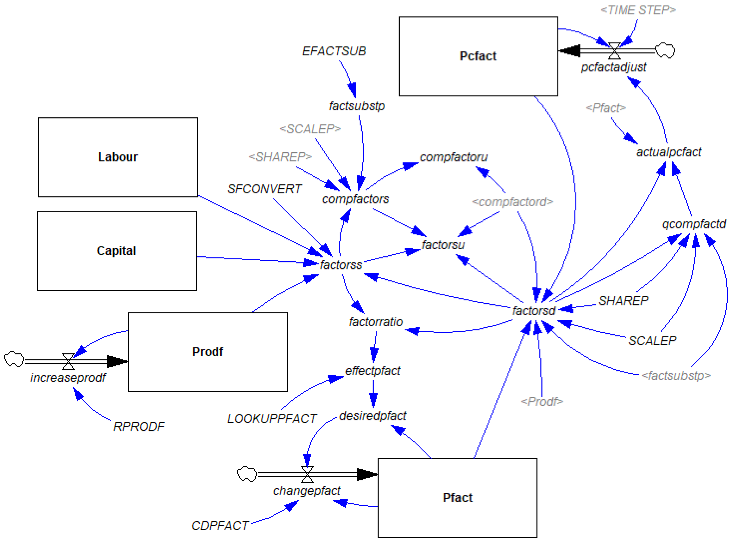
The Factors Module simulates, given total available supplies of labour and capital, the relative demand and supply of these factors to industries, and the dynamics of factor price changes (see Figure 4).
There are two sets of price stocks contained within the module, Pcfactj and Pfacth,j. While the former defines a composite factor price for industry j, taking account of the relative supplies of labour and capital to that industry and the respective prices of those factors, the latter is a specific price for factor h within industry j. The price stocks Pfacth,j vary in response to relative differences in the supply of factor h to industry j, and the demand for factor h by that industry, factorssh,j and factorsdh,j. The mechanisms through which these price change dynamics are implemented are analogous to those explained above (refer to Equations (S1)–(S5) in the Supplementary Material).
The producers within the economy (represented by industries) generate economic outputs subject to their production technologies. The technologies defining inputs of intermediate goods and composite factors are explained under the Commodities Module. Moving now to the next layer of the production nest, the technologies underpinning composite factor supply within each industry, compfactorsj, are represented by a CES function consisting of labour and capital factor endowments (Equation (25)). The factsubstpj parameters in this CES function depend on exogenously derived elasticities of substitution between the labour and capital factor inputs, EFACTSUBj (Equation (26)), while SCALEPj and SHAREPh,j are, respectively, the CES function scale and share parameters.
The Factors Module also incorporates an ability to include exogenous technological change; leading to improved efficiency in the utilisation of labour and capital. This is incorporated by way of productivity stocks for each factor h, Prodfh, which grow in accordance with an exogenous rate of productivity growth, RPRODFh (Equations (27) and (28)).
Recalling that the DES CF model is analogous to a comparative static CGE, the total stocks of capital and labour are set exogenously. Factor stocks are typically set as either fixed to certain industries (i.e., immobile) or free to move between industries (i.e., mobile), depending on the length of time for the analysis. Stocks of capital are therefore defined specific to industries, Capitalj, while the labour stock, Labour, has no subscripts. The effective supply of capital to each industry can now be determined simply by multiplying available capital stocks by Prodfcap and SFCONVERTcap (Equation (29)). The latter converter translates capital, thus far measured as a stock, into a flow measure. A similar approach is also taken to translate the labour stock into industry labour endowments (Equation (30)). As labour is however mobile across industries, the total supply of labour must also be shared among industries according to each industry’s relative demand.
Turning now to the demand-side of the module, following the principle of profit maximisation, industries will choose to utilise a combination of labour and capital inputs that meet the required total production level of composite factors, while minimising costs. Just like the approach described above to determine the relative input of factors versus intermediate goods, the first-order conditions for this problem enables a function to be generated that specifies each industry’s desired consumption of labour and capital, given relative differences in factor price (Equation (31)). As per the Commodities Module, it is necessary to continuously update the composite price (Pcfactj) to enable the CES function to effectively allocate total factor input demands among labour and capital. Adjustments to this composite factor price occur in an analogous manner to that described within the Commodities Module (see Equations (S6)–(S9) in the Supplementary Material).
The converter compfactoruj defines (see the Commodities Module) the actual consumption of composite factors by industry j. Note that compfactoruj may vary from the desired consumption of composite factors by industry j, compfactordj, where the supply of composite factors to the industry is insufficient to meet demand. Composite factor use can also vary from supply, compfactorsj, where there is an over-supply or surplus (Equation (32)). It is further necessary to define the quantities of each factor used by each industry, factorsuh,j, as these values feed into the income and tax calculations under the Households and Government Modules, respectively (Equation (33)).
2.3.4. Government Module
A relatively straightforward approach is taken in the construction of a Government Module (see Figure S3 in the Supplementary Material). A single stock, Govtaccount, keeps track of available government funds, receiving additions of disposable government income, govtincome, and subtractions from government expenditure, govtexpend (Equation (34)).
The value of govtincome is determined by the sum of the various taxes received. The underlying SAM will normally determine the types of taxes that need to be included. The relevant taxes are on factors, factortax representing factor tax and TAXFACTh the factor tax rate, prodtax representing production tax and TAXPRODFj the associated tax rate, and hhldtax representing household consumption tax and TAXHHLD the associated tax rate (Equations (36)–(38)). The converter hhldexpend captures the total expenditure by households on the consumption of goods and services and is defined under the Households Module. The remaining converters in these equations are explained previously.
In constructing the Government Module, there is a reasonable amount of discretion available in the choice of converters that may be set exogenously. CGE modellers often referred to these choices as “model closure”. Here it is assumed that the government sector always clears its available funds (Equation (39)), a fixed value from within these available funds, GHTRANS, is transferred to the household sector, and another fixed value is also transferred to savings, GOVTSAVINGS. Furthermore, of its available expenditure, the government sector uses a fixed proportion of purchasing each i commodity. These exogenous purchase rates, GCSPi, along with current commodity prices therefore determine the total quantity of each commodity consumed, govtconsumpi (Equation (40)).
2.3.5. Investment and Savings Module
The Investment and Savings Module has a similar structure to the Government Module (see Figure S4 in the Supplementary Material). It has a central stock of funds, Savingsaccount, which in this case receives additions from savings and subtractions from investment (Equation (41)). The value of total savings, savings, is calculated from the sum of government savings, GOVTSAVINGS, factor income saved, fincomeinvest, and household savings, hhldsavings (Equation (42)). The closure rules applied in the case of the household sector are relatively straightforward, with total household savings during a period calculated by multiplying the household income during that period, fewer taxes, by a constant household propensity to save, SSP (Equation (43)). Similarly, the value of factor income transferred to savings is determined by multiplying factor income, fewer taxes, by a constant exogenous rate for each factor, RFISTRANSh (Equation (44)). The converters dispfactincome and factorincomeh are defined under the Households Module.
Turning to investment, the total value of investment expenditure during a period is simply set equivalent to Savingsaccount, to achieve clearing of the available investment funds (Equation (45)). Assuming simply that fixed proportions of investment expenditure are allocated to each i commodity, ICSPi, and applying current commodity prices, the quantity consumed of each commodity, investconsumpi, is calculated as per Equation (46).
2.3.6. Households Module
The Households Module provides the final component of the model (see Figure S5 in the Supplementary Material) and, again, it has a structure like the Government Module.
The stock Hhldaccount receives household disposable income, disphhldincome, and provides expenditure for household consumption, hhldexpend (Equations (47) and (48)). The value of disphhldincome is calculated from the sum available income from factors, dispfactorincome, and household transfers from government, fewer household taxes and household income transferred to savings (Equation (49)). In turn, dispfactorincome is defined as the total income from factors (Equation (50)) less factor income transferred to savings (Equation (51)). Finally, a very simple household consumption function is applied that is analogous to those used in the case of the Government and Investment and Savings Modules (Equation (52)). The variable HCSPi defines the exogenous share of household consumption expenditure allocated to commodity i.
2.4. The Dynamic Equilibrium-Seeking Model with Factor Growth (DES FG)
The model may be extended to include growth dynamics through labour and capital stock changes. The System Dynamics approach is very convenient for incorporating such changes, as it allows for the values of capital and labour stocks to be are updated continuously, rather than in a stepwise fashion with an assumed equilibrium at the end of each period, as per many dynamic CGE models. Specifically, two additional modules, encompassing labour and capital dynamics, are introduced (see Figures S6 and S7 in the Supplementary Material).
2.4.1. Labour Module
Ever since the commentary of Sen (1963) [47], the problem of labour market closure has been a major focus, invoking an extensive controversial theoretical debate in the CGE modelling literature. Typically, a modeller has a choice between (1) assuming that the economy’s labour supply is exogenous, and an endogenous wage adjusts until national labour supply and demand are equal (often referred to as the “Neoclassical closure rule”), or (2) assuming that the economy-wide wage is exogenous, and an endogenous labour supply adjusts until labour supply and demand are equal (often referred to as the “Keynesian closure rule”). Even with the case-specific adaptions and modifications that can be made to these assumptions, for most real-world situations neither approach is entirely satisfactory. As this paper is concerned with modelling a closed economy rather than an open economy where there are possible movements of labour in, and out, of the system, labour is simply set exogenously. The total stock of labour is thus modelled by applying a set labour growth rate, LGR (Equations (53) and (54)), based on projected future population growth. Note also it is not a condition in the model that labour is necessarily fully employed.
Although labour is in principle a mobile factor of production, with persons able to move between firms and even industries to achieve the highest rates of compensation, in practice labour mobility is constrained by the relative supply of, and demand for, skills. There are several possible options for incorporating these dynamics. We choose to disaggregate the available labour force according to a set of identified skills or occupations. The total stock of labour is responsible for supplying to each of the different types of skills, but because of differences in education and training requirements, there is imperfect substitution (strictly speaking, “imperfect transformation”) in supply. This is represented through a Constant Elasticity of Transformation (CET) function (Equations (55) and (56)) where the total supply of labour of skill p, skillsp, is determined by the wage rate for that skill, Pskillp, relative to the economy-wide wage rate, as well as the elasticity of transformation of supply, ELABTRANS. The terms SHARELp and SCALEL represent the CET share coefficients for skill p and the associated scale coefficient.
Having determined the supply of a labour skill, the economy-wide price (i.e., wage) for that skill fluctuates, depending on relative differences between supply and demand, in much the same manner as other price dynamics in the model (see Equations (S10)–(S14) in Supplementary Material). The demand for a selected p skill, skilldp, is determined by total labour factor demands by industries (Equation (57)), as derived above under the Factors Module. The fixed coefficient SKILLSHAREp,j defines the amount of labour with skill p required by industry j, relative to total labour demand by industry j. As explained above, it is also necessary to incorporate the scalar, LSFCONVERTp, to translate labour as a flow measure from the Factors Module, into labour as a stock measure. Note that it is the factorsh=lab,j converter that constitutes inputs from the Factors Module into the Labour Module, and the converter indskillsp,j, defining the total supply of labour skill p to industry j, that forms inputs from the Labour Module back into the Factors Module. This latter converter is calculated by distributing the total supply of each p skill across all j industries, according to each industry’s share of the total demand for that skill (Equation (58)). Finally, to account for the introduction of labour skills to the model, Equation (30) from the Factors Module is replaced with Equation (59).
2.4.2. Capital Module
While some forms of capital are mobile between industries (e.g., office space, cash funds), other forms of capital (e.g., machinery, equipment) have very limited mobility. To incorporate these dynamics, the stock of capital held by each industry is modified to include: (1) the addition of new capital occurring either by way of investment or through transfers of mobile capital from other industries, (2) depletion of old capital through depreciation of existing stocks, and (3) loss of mobile capital to other industries (Equation (60)). Depreciation on capital stocks of industry j, depreciationj, is calculated simply by assuming a constant depreciation rate, RDEPj (Equation (61)). Similarly, the quantity of capital held within each industry that is mobile and potentially reallocated to other industries, mcapitalj, is determined by a constant capital mobility rate MOBILESHj (Equation (62)).
To remove the effect of commodity price changes in determining the relative quantity of new capital items, the investment undertaken in each period is divided by the current capital price, pcomdi (Equation (63)). Having determined the quantity of new capital items, they are distributed amongst industries according to endogenously derived industry shares, indshareinvestj (Equation (64)). A zealous specification of the model would allocate investment to industries according to each industry’s share of total capital income. These shares are defined by capitalincomeshj (Equation (65)). Recognising that investment is mobile across industries, the equation defining indshareinvestj also includes a set of terms that adjust investment shares to account for differences in capital returns (Equations (66)–(68)). Industries with above-average capital returns receive a larger share of investment funds than their share in capital income, while the converse occurs for industries from which capital returns are below average. The exogenous term INVESTMOB represents the proportion of total investment that is mobile between industries.
3. Results
This section illustrates the patterns of behaviour that can be generated by the DES CF and FG models. To facilitate understanding a very simple example is formulated that involves just two economic industries (Ind1, Ind2), each producing one unique type of commodity (Com1, Com2) and utilising two types of labour inputs to production (Skilled, Unskilled). For simplicity, it is also assumed that all capital is immobile between industries (for all j, MOBILESHj = 0), and the possibility of substitution between intermediate goods and factors is ignored.
The initial conditions for both versions of the DES model are determined from a global SAM derived by aggregating all 113 individual SAMs contained within the Global Trade Analysis Project (GTAP) 7.0 database.1 The majority of the exogenous constants (e.g., tax rates, government-household transfers) are obtained directly out of this dataset and are set as constant throughout the simulation. Additionally, for demonstration purposes, the elasticities for factor substitution and labour transformation are all arbitrarily set as 2, and the SHARE and SCALE parameters are determined via a calibration process (refer to [6] for a step-by-step guide to calibration). It is also important to note that the exogenous capital depreciation rate, RDEP, in both DES models is set so that the quantity of capital depreciated at the base year is equal to the quantity of new capital purchased. This assumption enables us to examine the behaviour of both DES models in terms of equilibrium growth paths following an exogenous shock.
3.1. Results without Exogenous Shock
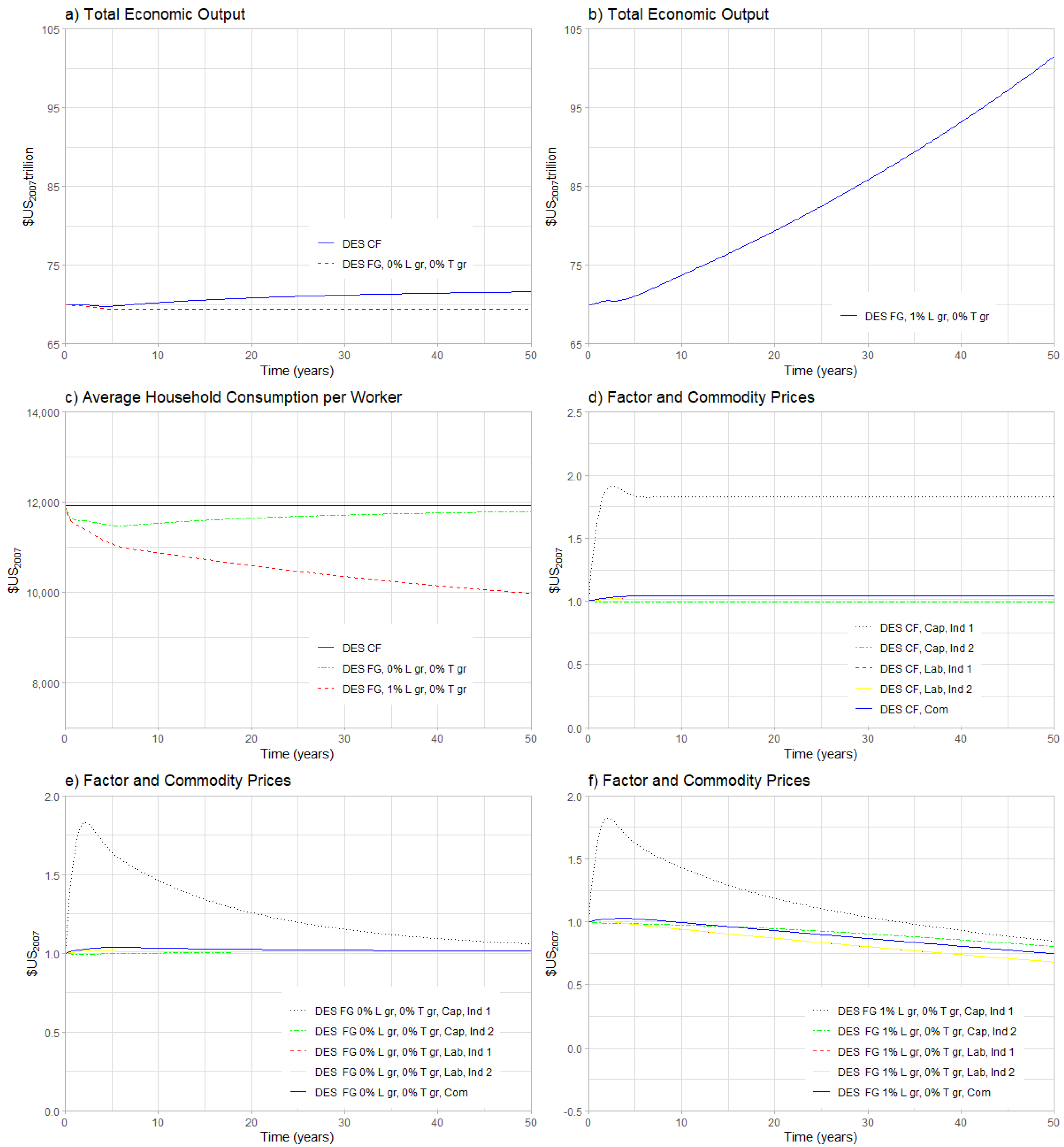
The results begin by showing the dynamics of each model with no exogenous changes or shocks introduced. Since each model starts at a position where new industry capital is equal to depreciation, and the labour force and productivity growth rates are set to zero, both models produce a steady-state situation where each endogenous variable remains at its base year value, i.e., the growth rate of labour and technological progress is set to a growth rate of 0% yr−1 (refer to Figure 5 “DES CF and DES FG result with 0% L gr, 0% T gr”). Figure 5b,c also depict the behaviour of the DES FG model when (1) a labour growth rate of 1 % yr−1 is introduced (“DES FG, 1% L gr, 0% T gr”), and (2) a labour growth rate of 1 % yr−1 is combined with an increase in the state of technological progress over time (“DES FG, 1% L gr, 0.5% T gr”). This latter adaptation is incorporated by way of a rate of productivity change of 0.5 % yr−1 that augments a firm’s capital endowment.
When a positive labour-force growth rate is applied in the DES FG model this continuously drives down the price of labour in Figure 5c. The price of capital also reduces, although to a lesser extent than the price of labour, because labour-for-capital substitutions reduce the demand pressures on capital. However, following the principle of diminishing marginal productivity, which places limits on how much output can be produced from a set level of capital simply by adding more and more workers, the total rate of economic growth cannot keep pace with the rate of increase in labour. Per capita incomes and expenditures thus start to decline, despite the continued absolute increase in economic output. Notice that over time this effect starts to fall away, because the amount of new capital created each period begins to outstrip the amount that is lost through depreciation. Effectively, this is made possible because declining commodity prices enable greater levels of capital to be purchased at lower costs. When the timeframe for analysis is pushed out sufficiently far, the system will eventually reach an equilibrium state where the rate of growth in the capital stock is enough to meet the rate of growth in labour. Commodities consumed per worker becomes constant, and with constant returns to scale in the CES production function, output growth is equivalent to the rate of growth in labour. If we now add the concept of exogenous productivity or technology change to the model dynamics, the system can reach a pathway where the rate of growth in output is above the rate of labour force growth and, hence, the exponential growth in per capita household consumption (Figure 5b, DES FG, 1% L gr, 0.5% T gr).
3.2. Results with Exogenous Shock
For exposition purposes, reference is again made to a simple example involving just two industries, two commodities, and two labour types. This time, however, the stock of capital held by Ind1, which is the smaller of the two industries producing around 10 percent of total economic output, is adjusted down by 50 percent in the initial base year (Figure 6). This may represent a scenario of a natural hazard event, for example, involving widespread damage to buildings, machinery, and other capital held by that industry.
Starting with the DES CF model, the economy is heavily constrained in the quantity of economic output that can be produced (Figure 6a). The initial period of impact is characterised by ongoing tightening of these constraints because Ind1 (which produces less output per unit of labour input than Ind2) substitutes labour for lost capital and, hence, demands a greater share of the available labour. Factor prices rise from the outset due to shortages in supply, reaching a peak at around year 2 (Figure 6d). Then from that point onwards, with reduced commodity demands from households and from industries, factor demands are generally in line with available factor supply. Eventually, the model tends towards a new equilibrium state where total output is around 3.8 percent lower than that of the base year situation, and per capita household consumption is around 3.4 percent lower (Figure 6a,c).
To demonstrate the impacts of adding capital accumulation, Figure 6 also shows the outputs of the DES FG model once the capital shock is incorporated. So that these results can be easily compared with those of the DES CF model, we start by examining outputs where the labour force and productivity growth rates are all set to zero (DES FG, 0% L gr, 0% T gr). While both models exhibit similar behaviour following the exogenous shock, the important difference is that the DES FG model tends towards a new equilibrium that is characterised by higher economic output and consumption levels than that of the DES CF model (Figure 6a,c). This outcome is understandable when one considers the different treatment of capital between the two models. Under the DES CF model, there is no process for accounting for capital stock changes, and thus capital loss from the system via the economic shock is lost forever. By comparison, under the DES FG model, because investment expenditures are fully balanced by the formation of new capital, and new investment can concentrate in the industry paying the highest return, over time the initial capital lost from Ind1 can be recovered. Eventually, if we push out far enough, the DES FG model will return to the pre-shock equilibrium. This implies that when attempting to evaluate the impacts of some type of economic shock, the pathway for an adjustment that the system may follow, and the length of time over which this may occur, may be just as important as the new equilibrium position.
Following on from this last point, Figure 6b,c,f respectively show the effect on economic output, average consumption per worker, and prices when the economic shock is applied in the context of ongoing labour force growth of 1 % yr−1. Note that these results for total economic output are presented in a separate graph from the previous examples, due to scale differences. Once again, the system behaves in a similar manner following the exogenous shock with a peak in the capital factor price for the directly impacted industry at around year 2. This time, however, the behaviour occurs against the background of increasing labour availability but diminishing marginal productivity. Within a relatively short time, the system returns to the same equilibrium growth path that characterised the pre-shock version of the model.
4. Discussion
While the DES model described above adopts many of the features that have become common in CGE models, it will be clear that there are some important distinctions. CGE models are specifically designed to determine the conditions under which an economic system can be said to be “in equilibrium”. By contrast, the emphasis of the DES model is on simulating behaviour changes or transition across time. While the DES model incorporates negative feedback relations that regulate behaviour and tend to cause the system to seek equilibrium, an equilibrium will not necessarily be reached during a simulation. Indeed, because a modelled system evolves over time, and can be influenced by ongoing changes in external conditions, the so-called equilibrium may be a moving target that we never expect to be reached. We can, for example, easily imagine that instead of a constant labour growth rate, as applied in the examples contained within Figure 5 and Figure 6, we could assume a more realistic constantly changing rate of labour growth, and in this case the DES model would not tend towards the same equilibrium growth paths as depicted in those figures.
From a practical point of view, the avoidance of an optimisation or mathematical programming procedure to solve the model, as is applied in the DES model, can be quite helpful. In many real-world applications, economic models will need to interface with other system models, e.g., demographic, socio-economic and environmental. The System Dynamics approach from which the DES model is constructed (based around stocks, flows and feedback structures) is a general approach that can be used for representing all sorts of dynamic systems. This includes, for example, more nuanced tracking of labour occupations and skills, depletion and degradation of natural resources, and decomposition of multi-capital and wellbeing impacts by societal segments. This capability facilitates analysis of emerging initiatives on green economies and social corporate responsibility [48].
A model such as the DES model may also have certain advantages over other approaches, depending on the model purpose. This can range from simply helping to generate an understanding of system behaviour through time for multiple stakeholders, for scoping problems and agenda-setting, through to comparison of broad policy choices, and selecting among options. If the principal objective is more towards fostering a general understanding of systems, it is best to avoid a modelling approach that is highly complex and expert oriented. The System Dynamics approach is supported by several software packages, the most notable being STELLA® (ISEE Systems, Lebanon, NH, USA; www.iseesystems.com), Vensim® (Ventana Systems, Harvard, MA, USA; www.ventanasystems.com), Powersim StudioTM (Powersim Software, Nyborg, Norway; www.powersim.com) and Insight Maker (www.insightmaker.com). These software resources greatly simplify the process of model development and iteration, to the extent that only basic programming and mathematical skills are needed to construct models. This, as well as the visual analytics tools of System Dynamics software (e.g., causal loop diagrams, causal tree diagrams, variable graphing), avoids the black box nature often characteristic of many economic models, permitting policymakers and other stakeholders to interactively explore the outcome of policy options. The time path trajectories produced by the System Dynamics approach facilitates users to envisage the interplay of causes and feedback structures underpinning model outcomes. Any erratic or unstable behaviour is obvious and will quickly force model users to re-evaluate core assumptions.
As the purpose of this paper is simply to introduce this alternative type of economic model that can expand our toolkit for representing and exploring economic systems, the DES model presented is deliberately kept simple and tractable. For example, in the household consumption function, there is no distinction between commodities necessary to satisfy basic needs and luxury items, and factors that may cause a change in the rate of savings are not considered. Nevertheless, for many purposes, the model will be enough, or in any case, it provides the basic building blocks that can be further refined for future simulations as appropriate.
One of the most obvious places for development is to modify the DES model so that it represents an open economy subject to international trade in commodities. In CGE models the treatment of interregional imports is typically represented by the so-called Armington approach, which allows for quality variations between imports and domestically produced goods, and substitution between domestic and imported goods in response to changes in relative prices [49,50]. Along with the Armington structure, we can further add an exchange rate (stock) to the model that changes over time in response to the relative imbalance between the supply and demand for the national currency, with imports and exports being a significant source of supply and demand, respectively. Importantly, by adding such features the DES model will represent further balancing or self-regulating feedback structures within an economic system. Another significant development is the alteration of industry production structures to allow for joint production. Essentially this can occur by adding additional CET functions within the model, enabling industries to alter relative commodity supplies in response to changes in relative commodity prices.
A key contribution of the DES model is the conceptualisation of prices as stocks that accumulate or diminish over time in response to discrepancies between supply and demand. In terms of future contributions, it is the authors’ opinion that there is significant potential to draw more on perspectives from Evolutionary Economics and potentially Agent-Based Modelling to inform the way in which economic behaviours are formalised within the model. Already evolutionary approaches are helpful in explaining some of the aggregate phenomena commonly incorporated within economic models, for example, evolutionary models of economic growth fueled by technical advance are useful for helping to explain aggregate changes in labour or factor productivity (cf. [51,52]). We also note that recent research has been focused on the behaviour of economic systems following (natural hazard) disruptive events. Here we see that an evolutionary perspective might provide some useful heuristics to help explain and justify modelling assumptions around the adaptation of economic systems following an event, such as changes in input structures or technologies of production observed at a whole-of-industry level.
Related to the preceding paragraph, key future development in the DES model is likely to relate to the re-evaluation (and potentially relaxation) of the income-expenditure equality constraints normally applied to economic agents, which imply that agents are continuously optimal, towards behavioural rules that might be better described as adapting routines. In the real-world agents do experience some variation between income and expenditure. This is evidenced by fluctuating inventories, drawing down and accumulation of cash reserves, and even the presence of unused or discarded outputs. System Dynamics has long recognised the concept of information delays underpinning system behaviours [40] and has developed model structures to incorporate these dynamics (refer, for example, to the exponential smoothing approach outlined by [41]). Information delays are recognised to occur wherever a decision that forms part of the causal structure of a system is influenced by gradual adjustments of perceptions or beliefs. By drawing on these structures it would be possible, for example, to allow agent’s decisions about production levels (and expenditure) to be based not just on the immediate level of demand and value of sales for their commodities (which could be atypical immediately following an external shock), but rather some type of average or expected level of demand and sales, based on recent experiences and adapting as experiences unfold.
Key next steps for the development of the DES FG include comparative studies with existing dynamic CGE models (e.g., recursive dynamic, sequential dynamic implementations) along with developing model calibration and validation procedures. Comparative studies provide an opportunity to not only better understand how the DES FG compares against conventional dynamic CGE models, but also showcase strengths and identify potential weaknesses. Such comparative studies also provide opportunities for extending the “building blocks” outlined to construct more nuanced models of economies and policy applications. The DES CF and FG models, like most CGE models, rely on SAMs to provide calibrated initial conditions for many model parameters. Nevertheless, this approach inherently assumes equilibrium. Of course, if an economy is out-of-equilibrium, as we argue is often the case, then developing alternative approaches to parameter estimation is also an important next step. Finally, it essential that procedures be developed for validating the DES FG. Interestingly, these procedures will likely combine existing approaches used within both dynamic CGE, and more generally, System Dynamics modelling. We are hopeful that this may produce new insights into macroeconomic model validation practices.
5. Conclusions
Models help us to make sense of complex systems without being overwhelmed, by forcing us to identify and describe key system processes and causal mechanisms. As a support tool for decision making, modelling helps to generate a general understanding of system behaviour across a variety of stakeholders, via systematically asking questions and defining new conceptions. Broad policy choices can be evaluated and compared to identify possible trade-offs or synergies. With enough information, testing and calibration, models can even be used to compare and help select among specific policy options or strategies.
The motivation for constructing the DES model described arose out of a desire to further expand the modelling toolkit available, with a focus on applications where, like IO and CGE models, interrelationships and interdependence within an economic system are important. Essentially a System Dynamics model is a computer-aided simulation model of a dynamic system consisting of a set of coupled, first-order differential equations. Simulation of the system is achieved by partitioning simulated time into discrete intervals and stepping the model through the simulation one interval at a time. This means that with appropriate model formulation and calibration, the DES model can potentially inform us not only of the conditions existing at the so-called equilibrium towards which the system moves, but also the nature of the transition path towards that equilibrium.
The equilibrium-seeking behaviour of the DES model is itself a manifest of the explicit incorporation of supply, demand and price relationships within the model. System models such as the DES model can be viewed in terms of causal diagrams that incorporate feedback loops. It is the presence of at least one dominating balancing feedback loop that causes a system to gravitate towards some form of equilibrium. The DES introduces the possibility for integration of the System Dynamics approach, with its focus on the identification and representation of balancing and reinforcing feedback structures within systems, with an empirical economic model that, like IO and CGE models, is structured for the consideration of whole-of-economy interactions. Significant opportunities now exist, we believe, to expand this line of enquiry.
Supplementary Materials
The following are available online at https://0-www-mdpi-com.brum.beds.ac.uk/2079-8954/8/4/42/s1 (a) Equations (S1)–(S14); (b) Supplementary figures Figure S1: Commodities Module Stock-Flow Diagram, Figure S2: Industries Module Stock-Flow Diagram, Figure S3: Government Module Stock-Flow Diagram, Figure: S4 Investment and Savings Module Stock-Flow Diagram, Figure S5: Household Module Stock-Flow Diagram, Figure S6: Labour Module Stock-Flow Diagram, Figure S7: Capital Module Stock-Flow Diagram); (c) an index of stocks, flows and converters used in the DES; and (d) folders that provide: (1) the underlying Social Accounting Matrix, with calibration calculations, that provides the model’s initial conditions (“SAM.xlsx”), (2) the Vensim® program code and simulation runs for the DES CF (“DES CF.mdl” (program code), “CF Model.vdf” (simulation run results) and “CF Model 50% capital.vdf” (simulation run results)), (3) the Vensim® program code and simulation runs for the DES FG models (“DES FG.mdl” (program code), “FG 0% L, 0%T 50% shock.vdf” (simulation run results), “FG 0% L, 0%T.vdf” (simulation run results), “FG 1% L, 0%T 50% shock.vdf” (simulation run results), “FG 1% L, 0%T.vdf” (simulation run results), and “FG 1% L, 05%T.vdf” (simulation run results)). Please note that the DES CF and FG models were built and run in Vensim® DSS for Windows Version 7.3.5 Single Precision (x32).
Author Contributions
Conceptualization, N.J.M. and G.W.M.; Data curation, N.J.M.; Formal analysis, N.J.M.; Funding acquisition, G.W.M.; Investigation, G.W.M.; Methodology, N.J.M. and G.W.M.; Validation, N.J.M.; Writing–original draft, N.J.M. and G.W.M.; Writing–review & editing, N.J.M. and G.W.M. All authors have read and agreed to the published version of the manuscript.
Funding
This research was funded by the New Zealand Government’s Ministry of Business and Innovation and Employment (MBIE) under the ‘Transitioning Taranaki to a Volcanic Future’ (grant number UOAX1913) and the Resilience to Nature’s Challenges National Science Challenge (grant number GNS-RNC043).
Acknowledgments
The authors would like to thank Adam Rose, Price School of Public Policy, University of Southern California for his encouragement, reflections and comments on this paper during its development. The authors would also like to thank the anonymous referees for their comments.
Conflicts of Interest
The authors declare no conflict of interest.
References
- Begg, D.; Fischer, S.; Dornbusch, R. Economics, 6th ed.; McGraw-Hill: New York, NY, USA, 2000. [Google Scholar]
- Samuelson, P.A.; Nordhaus, W.D. Economics, 19th ed.; Irwin/McGraw-Hill: New York, NY, USA, 2010. [Google Scholar]
- Dixon, P.B.; Jorgenson, D.W. Handbook of Computable General Equilibrium Modeling; Elsevier: Amsterdam, The Netherlands, 2013; Volume 1A. [Google Scholar]
- Dixon, P.B.; Jorgenson, D.W. Handbook of Computable General Equilibrium Modeling; Elsevier: Oxford, UK, 2013; Volume 1B. [Google Scholar]
- Hosoe, N.; Gasawa, K.; Hashimoto, H. Textbook of Computable General Equilibrium Modelling: Programming and Simulations; Lagrave Macmillan: Hampshire, UK, 2010. [Google Scholar]
- Lofgren, H.; Harris, R.L.; Sherman, R. A Standard Computable General Equilibrium Model in GAMS. Microcomputers in Policy Research 5; International Food Policy Research Institute: Washington, DC, USA, 2002. [Google Scholar]
- Quesnay, F. Le Tableau Économique. Edited and translated to English by M. Kuczynski and R. L. Meek. 1972; Macmillan: London, UK, 1758. [Google Scholar]
- Walras, L. Elements in Pure Economics, Original Work Published, 1874th ed.; Richard D. Irwin: Homewood, IL, USA, 1954. [Google Scholar]
- Leontief, W. The Structure of the American Economy (1919–1929); Harvard University Press: Cambridge, UK, 1941. [Google Scholar]
- Debreu, G. Theory of Value; Yale University Press: New Haven, CT, USA, 1959. [Google Scholar]
- Arrow, K.J.; Debreu, G. Existence of an equilibrium for a competitive economy. Econometrica 1954, 22, 265–290. [Google Scholar]
- Arrow, K.J. An extension of the basic theorems of classical welfare economics. In Proceedings of the Second Berkeley Symposium on Mathematical Statistics and Probability; University of California Press: Berkeley, CA, USA, 1951. [Google Scholar]
- Debreu, G. The coefficient of resource utilization. Econometrica 1951, 19, 273–292. [Google Scholar]
- Johansen, L. A Multi-Sector Study of Economic Growth; North-Holland: Amsterdam, The Netherlands, 1960. [Google Scholar]
- Harberger, A.C. The incidence of the corporate income tax. J. Political Econ. 1962, 70, 215–240. [Google Scholar]
- Scarf, H. The approximation of fixed points of a continuous mapping. Siam J. Appl. Math. 1967, 15, 1328–1343. [Google Scholar]
- Scarf, H.; Hansen, T. The Computation of Economic Equilibria; Yale University Press: New Haven, CT, USA, 1973. [Google Scholar]
- Aminu, A. A recursive dynamic computable general equilibrium analysis of value-added tax policy options for Nigeria. Econ. Struct. 2019, 8, 22. [Google Scholar]
- Gesualdo, M.; Giesecke, J.A.; Tran, N.H.; Felici, F. Building a computable general equilibrium tax model for Italy. Appl. Econ. 2019, 51–56, 6009–6020. [Google Scholar]
- Bye, B.; Strøm, B.; Åvitsland, T. Welfare effects of VAT reforms: A general equilibrium analysis. Int. Tax Public Financ. 2012, 19, 368–392. [Google Scholar]
- Shoven, J.B.; Whalley, J. Applied General Equilibrium; Cambridge University Press: Cambridge, UK, 1992. [Google Scholar]
- Shoven, J.B.; Whalley, J. Applied general-equilibrium models of taxation and international trade: An introduction and survey. J. Econ. Lit. 1984, 22, 1007–1051. [Google Scholar]
- Ginsburgh, V.; Keyser, M. The Structure of Applied General Equilibrium Models; MIT Press: Cambridge, MA, USA, 1997. [Google Scholar]
- Bekkers, E.; Antimiani, A.; Carrico, C.; Flaig, D.; Fontagne, L.; Foure, J.; Francois, J.; Itakura, K.; Kutilina-Dimitrova, Z.; Powers, W.; et al. Modelling Trade and Other Economic Interactions between Countries in Baseline Projections. J. Glob. Econ. Anal. 2020, 5, 273–345. [Google Scholar]
- Francois, J.; Martin, W. Computational General Equilibrium Modelling of International Trade. In Palgrave Handbook of International Trade; Palgrave Macmillan: London, UK, 2013. [Google Scholar]
- Partridge, M.D.; Rickman, D.S. Computable general equilibrium (CGE) modeling for regional economic development analysis. Reg. Stud. 2010, 21, 205–248. [Google Scholar]
- Partridge, M.D.; Rickman, D.S. Regional computable general equilibrium modeling: A survey and critical appraisal. Int. Reg. Sci. Rev. 1998, 86, 741–765. [Google Scholar] [CrossRef]
- Knowling, M.; White, J.T.; McDonald, G.W.; Kim, J.H.; Moore, C.R.; Hemmings, B. Disentangling environmental and economic contributions to hydro-economic model output uncertainty: An example in the context of land-use change impact assessment. Environ. Model. Softw. 2020, 127, 104653. [Google Scholar] [CrossRef]
- Fujimori, S.; Iizumi, T.; Hasegawa, T.; Takakura, J.; Takahashi, K.; Hijioka, Y. Macroeconomic Impacts of Climate Change Driven by Changes in Crop Yields. Sustainability 2018, 10, 3674. [Google Scholar] [CrossRef] [Green Version]
- Ren, X.; Weitzel, M.; O’Neill, B.C.; Lawrence, P.; Meiyappan, P.; Levis, S.; Balistreri, E.J.; Dalton, M. Avoided economic impacts of climate change on agriculture: Integrating a land surface model (CLM) with a global economic model (iPETS). Clim. Chang. 2016, 146, 517–531. [Google Scholar] [CrossRef] [Green Version]
- Bergman, L. CGE Modeling of Environmental Policy and Resource Management. In Handbook of Environmental Economics: Economy and International Environmental Issues; North-Holland: Amsterdam, The Netherlands, 2005; Volume 3, pp. 1274–1305. [Google Scholar]
- Shibusawa, H. A dynamic spatial CGE approach to assess economic effects of a large earthquake in China. Prog. Disaster Sci. 2020, 6, 100081. [Google Scholar] [CrossRef]
- Botzen, W.J.; Deschenes, O.; Sanders, M. The Economic Impacts of Natural Disasters: A Review of Models and Empirical Studies. Rev. Environ. Econ. Policy 2019, 13, 167–188. [Google Scholar] [CrossRef] [Green Version]
- McDonald, G.W.; Cronin, S.J.; Kim, J.H.; Smith, N.J.; Murray, C.A.; Procter, J.N. Computable general equilibrium modelling of economic impacts from volcanic event scenarios at regional and national scale, Mt. Taranaki, New Zealand. Bull. Volcanol. 2017, 78, 87. [Google Scholar] [CrossRef]
- Rose, A. Macroeconomic consequences of terrorist attacks: Estimation for the analysis of policies and rules. In Benefit-Cost Analyses for Security Policies: Does Increased Safety Have to Reduce Efficiency? Edward Elgar Publishing Limited: Cheltenham, UK, 2015; pp. 172–200. [Google Scholar]
- Miernyk, W.H. The Elements of Input-Output Analysis; Regional Research Institute, West Virginia University: Morgantown, WV, USA, 2020. [Google Scholar]
- Miller, R.E.; Blair, P.D. Input-Output Analysis: Foundations and Extensions; Cambridge University Press: New York, NY, USA, 2009. [Google Scholar]
- Raa, T.T. The Economics of Input-Output Analysis; The Edinburgh Building; Cambridge University Press: Cambridge, UK, 2006. [Google Scholar]
- Zodrow, G.R.; Diamond, J.W. Dynamic Overlapping Generations Computable General Equilibrium Models and the Analysis of Tax Policy: The Diamond-Zodrow Model. In Handbook of Development Economics; North-Holland: Amsterdam, The Netherlands, 2013; Volume 2, pp. 743–809. [Google Scholar]
- Bala, B.K.; Arshad, F.M.; Noh, K.M. System Dynamics: Modelling and Simulation; Springer: Singapore, 2017. [Google Scholar]
- Sterman, J.D. Business Dynamics: Systems Thinking and Modeling for a Complex World; McGraw-Hill Higher Education: Boston, MA, USA, 2000. [Google Scholar]
- Forrester, J.W. World Dynamics; Wright Allen Press: Cambridge, MA, USA, 1971. [Google Scholar]
- Forrester, J.W. Urban Dynamics; MIT Press: Cambridge, MA, USA, 1969. [Google Scholar]
- Forrester, J.W. Industrial Dynamics; MIT Press: Cambridge, MA, USA; John Wiley and Sons, Inc.: Hoboken, NJ, USA, 1961. [Google Scholar]
- Ravelojaona, P. On constant elasticity of substitution–Constant elasticity of transformation Directional Distance Functions. Eur. J. Oper. Res. 2019, 272, 780–791. [Google Scholar] [CrossRef]
- Van der Mensbrugghe, D.; Peters, J.C. Volume preserving CES and CET formulations. In Proceedings of the 19th Annual Conference on Global Economic Analysis, Washington, DC, USA, 15–17 June 2016. [Google Scholar]
- Sen, A. Neo-classical and neo-Keynesian theories of distribution. Econ. Rec. 1963, 39, 46–53. [Google Scholar]
- Popescu, C.R.; Popescu, G.N. An Exploratory Study Based on a Questionnaire Concerning Green and Sustainable Finance, Corporate Social Responsibility, and Performance: Evidence from the Romanian Business Environment. J. Risk Financ. Manag. 2019, 12, 162. [Google Scholar]
- Nemeth, G.; Szabo, L.; Ciscar, J.H. Estimation of Armington elasticities in a CGE economy-energy-environment model for Europe. Econ. Model. 2011, 28, 1993–1999. [Google Scholar] [CrossRef]
- Armington, P. A Theory of Demand for Products Distinguished by Place of Production. IMF Staff Pap. 1969, 16, 159–178. [Google Scholar]
- Neild, R. The future of economics: The case for an evolutionary approach. Econ. Labour Relat. Rev. 2017, 28, 164–172. [Google Scholar] [CrossRef]
- Dossi, G.; Nelson, R.R. An introduction to evolutionary theories in economics. J. Evol. Econ. 1994, 4, 153–172. [Google Scholar] [CrossRef]
| 1 |
Figure 1.
Relationships between Commodity Supply, Demand, and Price.

Figure 2.
Price Stock-Flow Diagram for Commodities. CDPCOMS = change delay for commodity price, changepcoms = increase in commodity price, excesssupply = ratio of commodity supply to commodity demand, LOOKUPPCOMS = lookup function determining applicable price change effect, Pcoms = commodity supply price, productionc = commodity production, usec = commodity use.

Figure 3.
Commodities Module nested tree depicting supply of, and demand for, a representative commodity (Com1). CES = Constant Elasticity of Substitution.
Figure 3.
Commodities Module nested tree depicting supply of, and demand for, a representative commodity (Com1). CES = Constant Elasticity of Substitution.

Figure 4.
Factors Module Stock-Flow Diagram. Any variable contained within parentheses (“< … >”) is either defined in another module or exists elsewhere within the same module.
Figure 4.
Factors Module Stock-Flow Diagram. Any variable contained within parentheses (“< … >”) is either defined in another module or exists elsewhere within the same module.

Figure 5.
Outputs of DES Model without application of Exogenous Shock. DES CF = Dynamic Equilibrium-Seeking Model with Constant Factors, DES FG = Dynamic Equilibrium-Seeking Model with Factor Growth, L gr = per annum labour growth rate, T gr = per annum productivity growth.
Figure 5.
Outputs of DES Model without application of Exogenous Shock. DES CF = Dynamic Equilibrium-Seeking Model with Constant Factors, DES FG = Dynamic Equilibrium-Seeking Model with Factor Growth, L gr = per annum labour growth rate, T gr = per annum productivity growth.

Figure 6.
Outputs of DES Model without application of Exogenous Shock at Time=0. DES CF = Dynamic Equilibrium-Seeking Model with Constant Factors, DES FG = Dynamic Equilibrium-Seeking Model with Factor Growth, L gr = per annum labour growth rate, T gr = per annum productivity growth, Cap = capital, Lab = labour, Ind 1 = Industry 1, Ind 2 = Industry 2.

Publisher’s Note: MDPI stays neutral with regard to jurisdictional claims in published maps and institutional affiliations. |
© 2020 by the authors. Licensee MDPI, Basel, Switzerland. This article is an open access article distributed under the terms and conditions of the Creative Commons Attribution (CC BY) license (http://creativecommons.org/licenses/by/4.0/).
Share and Cite
MDPI and ACS Style
McDonald, N.J.; McDonald, G.W. Towards a Dynamic Equilibrium-Seeking Model of a Closed Economy. Systems 2020, 8, 42. https://0-doi-org.brum.beds.ac.uk/10.3390/systems8040042
AMA Style
McDonald NJ, McDonald GW. Towards a Dynamic Equilibrium-Seeking Model of a Closed Economy. Systems. 2020; 8(4):42. https://0-doi-org.brum.beds.ac.uk/10.3390/systems8040042
Chicago/Turabian StyleMcDonald, Nicola J., and Garry W. McDonald. 2020. "Towards a Dynamic Equilibrium-Seeking Model of a Closed Economy" Systems 8, no. 4: 42. https://0-doi-org.brum.beds.ac.uk/10.3390/systems8040042
Note that from the first issue of 2016, this journal uses article numbers instead of page numbers. See further details here.