Quantifying Risk Perception: The Entropy Decision Risk Model Utility (EDRM-U)


1
Department of Industrial, Manufacturing and Systems Engineering, Texas Tech University, Lubbock, TX 79409, USA
2
School of Engineering and Sciences, Tecnologico de Monterrey, Monterrey 64849, Mexico
*
Author to whom correspondence should be addressed.
Systems 2020, 8(4), 51; https://0-doi-org.brum.beds.ac.uk/10.3390/systems8040051
Submission received: 26 October 2020
/
Revised: 20 November 2020
/
Accepted: 30 November 2020
/
Published: 3 December 2020
Abstract
:Risk perception can be quantified in measurable terms of risk aversion and sensitivity. While conducting research on the quantization of programmatic risk, a bridge between positive and normative decision theories was discovered through the application of a novel a priori relationship between objective and subjective probabilities and the application of Bernoulli’s expected utility theory. The Entropy Decision Risk Model (EDRM) derived using the Kullback–Liebler entropy divergence from certainty serves as a translation between objective and subjective probability, referred to as proximity, and has proven its applicability to various positive decision theories related to Prospect Theory. However, EDRM initially assumes the validity of the standard exponential power utility function ubiquitous to positive decision theory models as the magnitude of a choice to isolate and validate proximity. This research modifies the prior model by applying Daniel Bernoulli’s expected utility as the measure of choice magnitude in place of power utility. The revised model, EDRM Utility (EDRM-U), predicts the subject choices for both small and large ranges of values and shows that Prospect Theory’s neutral reference point is actually centered about an assumed initial wealth value, called neutral wealth, that correlates to a power utility exponent value. This hypothesis is confirmed by demonstrating that EDRM-U presents an equivalent or better correlation with prior research in eleven landmark studies of college students spanning more than 26 years and comprising over 300 problems, including those with widely varying values. This research contributes to the fields of risk management and decision engineering by proposing a decision model that behaves according to both positive and normative decision theories and provides measures of risk perception.
1. Introduction
Three oil industry CEOs are playing penny-ante poker, each with several dollars of holdings. Are they making risk decisions based upon their billions in assets? Surely not. They are playing with the money in front of them. However, the next day they are deciding how to leverage hundreds of millions of dollars to gain market share over one another. Are the same decision processes at work? Up until now, the answer would be, no, but this research will show how the answer can be yes.
Daniel Bernoulli’s expected utility (EU) is the foundation of the rational-agent model for risk decisions; however, it has been shown to be inconsistent with the results from numerous studies of subject choice—how people actually make decisions. The reflexive assumption has been to acknowledge the validity of the findings but then conclude that subjects are to some degree irrational, thereby preserving the bulwarks of rational decision theories, but could both be true at the same time? This research proposes that the differences between the normative and positive decision theories can be resolved by building upon the Entropy Decision Risk Model (EDRM), which translates between the objective probabilities of normative behavioral economics and the subjective probabilities found in positivist theories (i.e., Prospect Theory), but uses power utility for magnitude and the harmonization of the concepts of initial wealth from EU and the neutral reference point of positivist decision making under uncertainty (DMUU) theories [1]. Daniel Kahneman, who pioneered Prospect Theory (PT) with Amos Tversky, identifies a contention with EU: “the [expected utility] theory fails because it does not allow for the different reference points,” (D. Kahneman, 2011, p. 276). Kahneman also asserts that happiness is based upon recent changes in one’s assets rather than absolute wealth—the basis for his neutral reference.
At first blush, this appears to be an insurmountable task of resolving the relative (neutral reference points) and the absolute (initial wealth), but this research reveals agreement by showing that the neutral reference point actually belies the initial wealth and that rational decisions made under EU can be based upon a perception of assets at a given moment in time rather that one’s net worth. The term “neutral wealth” is introduced as the combination of a neutral reference point and initial wealth. Neutral wealth is not a measure of actual wealth or the size of a gamble, but rather is a relative measure that varies by person, group, situation, or condition. Reversing an assumption made by Bernoulli, the wealthy may actually perceive a low value of neutral wealth and the poor a high value. For example, a large neutral wealth (insensitivity to risk) indicates spendthrift behavior, whereas small values may represent miserliness (sensitive to risk).
From a practical perspective, there is another significant disagreement between the two theories. While EU appears to work for supporting decisions involving large changes in wealth, positive decision theory studies are often conducted using items of small value (mugs, candy bars, and up to several thousand dollars) and do not scale when applied to major personal or corporate financial decisions; in other words, their usefulness is bounded. This research reveals that, by using neutral wealth in developing EDRM Utility (EDRM-U), the standard power utility applied to positive studies is functionally a subset of the logarithmic expected utility curve about neutral wealth. Subject choices over the full range of wealth or asset values can also be predicted or converted from the subjective domain into the objective for consistency with traditional rational economic choice analyses. Table 1 provides a comparison of the three models.
Practical Application Example (Notional)
An executive with a neutral risk aversion is playing penny-ante poker holding a pair of twos. He has already put $0.11 in the pot and needs to add another $1 to match the last bet and call. He assesses that he has a 50% chance of collecting $5, which includes the $1.11 he will have already played, and chooses to take the bet. The next morning, he has to decide between two options, both of which require an investment of $1M. The first choice is assessed to have a 10% chance of a gross return of $20M ($19M net), and the second has a 50% likelihood of returning $2M ($1M net). Despite the greater expected value of the more speculative option, he follows his instincts and chooses the $2M option, prioritizing the certainty of cash flow over a possible windfall.
The choices are stated below in standard format (value, probability). Probabilities of 1.0 are assumed if not stated.
- Part 1.
- Choice 1A: ($5, 0.5; −$1; −$1.11) (Selected) Choice 1B: (−$0.11).
- Part 2.
- Choice 2A: ($20M, 0.1; −$1M) Choice 2B: ($2M, 0.5; −$1M) (Selected).
Figure 1 shows the EDRM-U risk perception plot of risk aversion versus neutral wealth (risk sensitivity) for this problem. The white region shows a wide range of acceptable neutral wealth values for a neutral risk aversion (), where both the small value gamble and the business decision overlap. This result shows that the executive’s treatment of these two risk decisions is consistent.
2. Method
This research answers the question of whether choice decisions are actually based upon some form of initial wealth (EU), which would be contrary to assumptions made by positive decision theories such as Prospect Theory. The answer lies in the hypothesis that the commonly used exponential power utility is actually an approximation of logarithmic expected utility over a narrow range of values, which implies that choice decisions are made based upon actual or perceived initial wealth. When proven, this provides commensurability between positive and normative decision theory models.
EDRM using power utility, EU using objective probability, and EDRM-U using logarithmic expected utility are compared using data from eleven prior studies of college students over a 26-year period for validation, including those examining choices made with large changes in values, such as Prelec (1998) and Hershey et al. (1982). In total, there are 321 problems under analyses in Section 6, with a focus on the set of 259 uncertain economic choice problems. Both EDRM and EDRM-U will be shown to be generally consistent with von Neumann–Morgenstern utility, which will establish a common applicability to both positive and normative decision theories. It is important to note that this research is really contrasting power utility and expected utility using EDRM and EDRM-U, respectively. Saying that EDRM-U performs better than EDRM means that the expected utility outperforms the power utility when applied to behavioral economics studies using proximity as the probability measure.
In addition to comparing the binary choice results (matching: yes or no), where appropriate, calculated prospect values are translated to percentages representing subject response frequency using the Percentage Evaluation Model (PEM) for direct comparison with subject data through statistical analysis using several methods [1]. Optimizations are performed by first maximizing binary results and then by minimizing the standard deviation of the percent differences of matches. Agreements between the actual and calculated percentages are evaluated using standard deviations and regression coefficients—specifically, the coefficient of determination (R2) and the nonparametric Spearman Rank Test (). Summary analyses are also performed using ANOVA at a standard 5% significance level to determine if the types of problems and the magnitude of the values have a significant effect on the results for both EDRM and EDRM-U. Note, in this case, that the assumptions of independence and constant variance can be presumed and normality will be confirmed by the use of the Shapiro–Wilk test. A flowchart illustrating the present research is provided in Figure 2.
3. Literature Review and Application
Because of the need to construct the argument for EDRM-U using major concepts, the review of literature within each subsection is immediately followed by a discussion of its application.
The purpose of this literature review is to summarize the body of knowledge surrounding the two competing concepts of Bernoulli’s initial wealth and Kahneman’s neutral reference point [1]. Supporting this approach, German economist Hans-Werner Sinn, reversing from prior statements, wrote, “I must now admit that the case for a logarithmic expected utility function is stronger than I had thought…Bernoulli may have been right after all and Fechner’s interpretation of Weber’s law may carry over to the shape of the von Neumann-Morgenstern function is a much more direct way than could have been imagined” [2]. While Maurice Allais, a progenitor of positive decision theory, was highly critical of VNM utility theory, he did assert that utility can be based upon Weber–Fechner’s threshold [3]—EDRM-U does exactly that.
This research is founded upon Jeremy Bentham’s original definition of utility, which includes four primary factors: intensity or magnitude, duration, certainty or uncertainty, and proximity or remoteness [4]. The time (duration) factor will be addressed in the future, but the other three are the same as those recognized by Daniel Ellsberg in evaluating choices [1,5]. The first step of isolating the relationship between proximity and objective probability was accomplished in developing EDRM by first accepting the validity of power utility as a measure of intensity or magnitude ubiquitous to behavioral economics. The next step taken by this research is to then evaluate expected utility as the magnitude instead of power utility by modifying EDRM, continuing to use proximity in place of objective probability. The new model, EDRM-U, is the result of this evolution; however, EDRM remains valid for many prior behavioral economics studies with smaller ranges of values, as shown in Section 6.
3.1. Daniel Bernoulli’s Expected Utility
Daniel Bernoulli’s EU theory published in 1738 is seemingly as much foundational in economic decision theory and risk analysis as it is a target for criticism by those studying human behavior and DMUU. EU theory underpins most basic economic decision making tools, including rate-of-return, net present value, the capital asset pricing model, and others [6]; however, EU has been shown to not properly model many discrete choice problems. Despite the assumed lack of alignment with DMUU, Bernoulli’s paper also laid the groundwork for psychophysics, which relates physical stimulus to perception and mental response (i.e., Weber–Fechner Law) [7,8]. It would seem, based upon this fact alone, that EU should predict how subjects perceive choices in a decision.
EU is a simple logarithmic relationship based upon the notion that the change in perception is a function of the inverse of wealth, such that, as wealth increases, the utility of that wealth decreases, as shown in Figure 3 cited directly from Bernoulli’s paper, where wealth is on the horizontal axis and utility on the vertical. The utility is weighted by the probability of achieving a certain wealth [9]. Utility is the psychological value.
In his development and explanation of EU theory, Bernoulli used real socioeconomic and business examples to extract a logarithmic model to explain both lottery and insurance in terms of “utility” rather than price, which he characterized as two different regions of wealth on his utility curve [9]. Poor people with little wealth purchase lottery tickets and insurance because they are loss averse due to a lack of means; whereas, inversely, wealthy people sell lottery tickets and insurance.
Referring to Figure 4, Bernoulli provides the following relationship describing the expected final wealth based upon the combination of a set of probability-weighted “wealths.”
where AB represents the initial wealth; AP is the final wealth; AC, AD, AE, etc. are the “wealths” for each of the states under consideration. Each log ratio is the change in wealth from the initial wealth. is a common scaling factor for the slope of the logarithmic curve and the objective probabilities and weight each of the respective states. Note that the expected wealth, , is independent of since it is cancelled on both sides of the equation. In other words, the expected wealth is only dependent upon the curvature of the utility function and not its slope.
Comparison of Power Utility and Expected Utility
Despite the positivist views of DMUU that generally abjure and have sought to refute EU [8], elements of both are required to properly explain how subjects make choice decisions over a wide range of values. To begin, a comparison of the power utility and expected utility is necessary.
Figure 4 illustrates the idea that the exponential power utility can be viewed as a subset of the logarithmic EU plot for certain values of and neutral wealth, . As the neutral wealth is changed the slope also changes, so there is a corresponding value of the power utility exponent () that approximates the slope. Using the EU curve in this manner also naturally accounts for a degree of loss aversion.
The shape of the two curves is further analyzed in Figure 5, which compares the curvatures (2nd derivatives). In addition to the details discussed in the caption, this plot illustrates that the EDRM-U application of logarithmic utility is consistent with Prospect Theory, as it shows risk seeking for gains ( and aversion to loss ( [10].
3.2. Neutral Reference Point
Harry Markowitz introduced the concept of the “neutral reference point” in his paper, “The Utility of Wealth”, where he coined the term “customary wealth” and established an argument that risk behavior is “essentially the same whether he is poor or rich” because all subjects will at the same time buy insurance and then take gambles; however, Markowitz completes the thought with the following statement that becomes a foundation of this research: “except the meaning of ‘large’ and ‘small’ will be different,” as they pertain to both probability and magnitude [11]. Markowitz’s orthogonal characterization of risk behavior and perception of small versus large also helps form the basis of for risk perception, as discussed later. This distinction between large and small indicates that the very notion of the neutral reference point is not absolute by acknowledging that it is only valid over a limited range. Richard Thaler also alludes to the concept of neutral wealth in his discussion of reference outcomes [12].
In Prospect Theory, utilities are based upon changes in wealth condition rather than initial and final wealth states, which is in contrast with Bernoulli’s EU [8]; however, Kahneman and Tversky recognize the same limitation as Markowitz, opening the door to applying EU to EDRM when they write: “So far in this paper, gains and losses were defined by the amounts of money that are obtained or paid when a prospect is played, and the reference point was taken to be the status quo, or one’s current assets. Although this is probably true for most choice problems, there are situations in which gains and losses are coded relative to an expectation or aspiration level that differs from the status quo [10].”
Myriad studies have been conducted in this arena, but most represent small monetary values which are varied over a limited range of a few thousand dollars at most. As an example, experiments for Richard Thaler’s endowment effect were centered around consumer behavior involving college students with a meagre income buying and selling mugs and pens [13]. While not minimizing the importance of this landmark research showing the effect of ownership in setting one’s value of item (endowment), the small magnitudes being considered make extrapolation to the larger magnitudes found in businesses and corporations most difficult, if not invalid. Studies such as “Sources of Bias in Assessment Procedures for Utility Functions” by John Hershey et al. used a much wider range of values ($10 to $1M), which prove problematic for prediction using models applying power utility functions, such as EDRM, which does not work for smaller and larger values simultaneously [14]. From this, one can easily conclude that elements of both PT and EU are required to explain choice selection over a wide spectrum of values.
3.3. Entropy Decision Risk Model
EDRM provides a conversion between the positive and normative decision theory domains by translating between objective and subjective probabilities, respectfully referred to as “relative certainty” () and “proximity” (); proximity is the nearness to a state.
Decisions consist of two or more choices, and choices are made up one or more states [15]. A state is comprised of a magnitude and a probability. EDRM uses proximity as the probability and power utility for the magnitude. Statistical mechanics and information theory entropy (they are synonymous) are representative of human cognition, which was further demonstrated in EDRM derivation and validation [1,16,17,18]. Starting with basic state entropy from information theory or statistical mechanics in terms of subjective probability (proximity), , the Kullback–Leibler entropy divergence from certainty is calculated [19,20]:
This solves to the following non-invertible equality:
where is the relative certainty (an objective probability) and is the proximity (subjective probability). The relationship between relative certainty and proximity is illustrated in Figure 6 below, which nearly perfectly aligns with Cumulative Prospect Theory’s (CPT) decision weight curve (Section 5.3) [1,21,22].
Applying proximity to the magnitude yields the prospect () of individual choice states in terms of power utility times the proximity ( in the same form as that used in Prospect Theory (PT) [10]:
The exponential factors, and , shape magnitude ( and proximity, respectively. λ is the loss aversion factor and is equal to or greater than 1; it is shown here for consistency with PT and will be assumed to be a neutral value of 1 for this research, as loss aversion will be shown to be manifested as risk aversion (dependent upon β) in EDRM-U. For uncorrected EDRM, , by definition. Kahneman and Tversky used a value of in PT and CPT. Since choices are made up of sets of individual gains and losses, or “states”, the total prospect of a choice j is the sum of the individual states,
where is the number of states. The choice with the largest value of prospect (most positive or least negative) is preferred. EDRM makes two critical assumptions in analyzing the decision uncertainties pertaining to magnitude:
- It accepts the use of the power utility ubiquitous to positive decision theory research to isolate the subjective-objective probability relationship, as shown in Equation (4);
- It assumes there is no difference in how the subjects valued gains or losses (i.e., that the value function exponent was constant for gains or losses and that no loss aversion was present).
These assumptions enable the isolation of the uncertainty effects (proximity and relative certainty) for analysis and validation. The present research sets aside these assumptions in EDRM-U, which instead applies expected utility in place of power utility. By accepting the validated relationship between proximity and relative certainty using uncorrected EDRM in 63 problems of subject choice, which are all included here in this broader research, then the choice magnitudes can now be reconsidered for their alignment with EU theory and a loss aversion effect will be evidenced in the form of risk aversion [1,19,21].
3.4. Mental Accounting and Transaction Utility
Problems involving only losses are treated differently than those of only gains or mixtures of the two, and this section develops the basis for this difference. Expected utility is a valid function for “transaction utility”, which is founded upon the “merits” of a deal rather than the values of the goods and is referred to as “acquisition utility”. In “Mental Accounting and Consumer Choice”, Thaler describes four possible combinations of inequalities related to transaction utility [12], classifying them in terms of “segregation” or “integration”: segregation occurs when the sum of the parts is preferred to the whole, whereas integration prefers the whole to the total of the parts.
- Case 1
- Multiple gains (segregation): , which says that people prefer many smaller gains over a single larger gain (i.e., people like a greater number of smaller presents).
- Case 2
- Multiple losses (integration): ; affirms that subjects prefer grouped losses rather than separated ones (i.e., people prefer consolidated bills).
- Case 3
- Mixed gains (integration with cancellation): ; is always positive, but the losses more quickly cancel out gains due to loss aversion.
- Case 4
- Mixed losses (segregation or integration with cancellation): . Because is always negative and gains are felt less than commensurate losses, Thaler states that there is a point at which there is a shift between segregation and integration; the introduction of neutral wealth permits defining this shift point.
Each of these four cases is satisfied using any convex function, including a logarithmic value function (inverse hyperbolic sine will be used here) varying by neutral wealth such that and . This is consistent with the insurance problems presented by Bernoulli, showing it is preferable to split shipping cargos to limit the impact of losses, thus increasing the expectation of increasing wealth [9].
Employing the “asinh” value function, it becomes evident that the multiple gain case is met using a positive value of neutral wealth and the multiple loss case is met using a negative value; subjects prefer greater gains and lesser losses. Following the logic presented by Thaler, the mixed gain case 1 is always true for any positive value of neutral wealth. For the mixed loss case 2, this shift between segregation and integration occurs when neutral wealth equals the negative average of and , which solves the equality , for using the asinh value function. When is greater than this crossover value, then segregation applies and, when less, integration applies. The remainder of this section is devoted to fully developing this concept.
While the center of each of the figures presented by Thaler, shown in Figure 7, is assumed to be a neutral reference point, the shape of the curves belie the idea that the “origin” could actually be neutral wealth and that the difference in slopes accounting for loss aversion is actually the result in this shift in the axes of an “asinh” plot; x and y vary from the neutral wealth value or “origin.”
These observations are critical to this research because they define how problems of pure gains, pure losses, and mixtures of the two should be handled with respect to neutral wealth. Each of Thaler’s four cases are based upon the same equality:
By introducing the crossover wealth () as the boundary between segregation and integration preferences, the four cases can be analyzed in terms of neutral wealth. Applying the inverse hyperbolic sine function yields:
Solving for the segregation-integration crossover wealth () at :
Figure 8 illustrates the four cases with respect to the crossover wealth and the varying values of x and y.
The value of is important to providing insight into how neutral wealth is considered for the different problem types. Rather than seeing problems in terms of pure gains, pure losses, and mixtures of the two, the four cases can be expressed in terms of segregation or integration and whether or not problems are mixed gains and losses. Thaler applies the term cancellation to cases 3 and 4 involving gain/loss combinations because smaller losses or gains are seen as cancelling some of the larger gains or losses. The effect, as seen in Table 2, also reveals a reversal of the inequities for mixed problems where cancellation is present. This result shows that segregation and integration are not explicitly tied to gains and losses when a neutral wealth other than zero is used. For example, segregation can be preferred for a combination of multiple losses if the neutral wealth is large enough, which is inconsistent with Thaler’s predictions as answered below. Additionally, Table 2 and Figure 9 show that a value of aligns with Thaler’s reported calculations and models.
Figure 9 illustrates the effects of introducing neutral wealth into the transaction utility value function. In general, it is assumed subjects use a positive value of neutral wealth, for which cases 1, 3, and 4 are properly aligned with expectations for increasing values of ; however, case 2 is special and is reversed. If neutral wealth is increased above the crossover wealth, then case 2 shifts to segregation, which is inconsistent with expectations, perhaps due to subjects considering wealth only in terms of losses in the case of these pure loss problems. So, EDRM-U model development must account for this effect by reversing the sign of the neutral wealth for case 2; this effect is validated against actual results.
This reversing of the sign of neutral wealth for purely negative choices is also consistent with the standard positive theory application of power utility, which defines that negative values are treated the same as positive but with inverted signs, as expressed by Tversky and Kahneman’s power utility value function definition [22]:
where is positive and less than or equal to 1 and is positive and greater than or equal to 1 to account for loss aversion. Loss aversion is treated differently in EDRM-U, without a separate scaling factor, as seen in the analysis of the risk aversion parameter (see Section 6.3).
3.5. Gain-Loss Separability
Tversky and Kahneman state that Cumulative Prospect Theory satisfies gain-loss separability in a concept that they define as “double matching”. Specifically, they deduced that, for a mixed choice of gains and losses (, if the respective gain and loss states match, then the combination or coalescing of choices also match: [22]. However, the extension of the double matching axiom to the more general case where the decomposed gains and losses of all mixed choices are respectively compared against each other elicits differing subject responses. In their report, “An Empirical Test of the Gain-Loss Separability in Prospect Theory”, George Wu and Alex Markle conclude that gain-loss separability is violated for these cases when the choices are not equivalent. Michael Birnbaum and Jeffrey Bahra reach a similar conclusion in their research into the gain-loss separability and coalescing of choice states [25].
Based upon these studies, it can be concluded that subjects view gains, losses, and the combination of the two differently, which is reflected in the very differences between positive and normative decision theories and is analogous with the classical ideal gas mixing problems in statistical mechanics (physics). The positivist behavioral economics view is that pure gains and losses are mirrors of each other, scaled by a loss aversion factor. This mirror effect is also affirmed in the previous discussion regarding the sign reversal of the neutral wealth in Thaler’s case 2. The normative view is consistent with EU theory, which treats all losses as a greater change of utility than corresponding gains.
3.6. Risk Perception Measures: Risk Aversion and Risk Sensitivity
Lennart Sjöberg, in his paper, “The Methodology of Risk Perception Research”, concludes that the process of quantifying risk perception is one of simplification into measurable terms and that study in this area cannot proceed further without a simplified picture of the dominating themes [26]. This sentiment invokes the words of Lord Kelvin (Sir William Thomspson): “when you cannot measure it, when you cannot express it in numbers, your knowledge is of a meagre and unsatisfactory kind” [27]. This research proposes such a simplified measure of risk perception.
No discussion about the perception of risk in the making of decisions could begin without looking to the works of Paul Slovic, like many others (e.g., Rasmussen and Perrow) advancing the study of risk after it was realized that amazing technical advances, such as nuclear power, could have unprecedented consequences [28,29,30]. Slovic identified a taxonomy, the psychometric paradigm, to make quantitative representations (cognitive maps) of risk perceptions and attitudes as components of the risk affect heuristic [31]. There are a number of examples of subsequent research applying Slovic’s work to measure risk perception [32,33,34]. Later, in 2006 Slovic and Peters narrowed down risk perception into two categories: risk as feelings and risk as analysis, which comport with type 1 (fast, intuitive) and type 2 (slow, deliberate) thinking, respectively [8,35]. Risk perception measures need to include both categories.
Like Slovic and Peters, Sjöberg identified two factors for risk perception: risk attitude and sensitivity [36]. To illustrate, Table 3 shows a comparison of dual process theory, Slovic and Peters, Sjöberg, and the factors used in this research
“Risk aversion” and “risk sensitivity” emerge as concepts that directly relate to parameters already identified in the model. Risk aversion indicates how subjects perceive uncertainty, where a risk-averse person avoids uncertainty and one who is drawn to it is risk seeking. As a measure of risk aversion, the proximity exponent () relates to the nearness to risk. Differing from proximity, risk sensitivity is a measure of the perception of risk and will be ascribed to neutral wealth. To analogize using climate, some like cold climates but some hate being cold and bundle up; they are both cold seeking and averse to cold weather. Differing from their preference in temperatures, some are sensitive to cold while others are insensitive (this is explored further in Section 3.6.2). These definitions are supported by further analysis.
Supporting this idea of defining two orthogonal factors to define risk perception, Peter Wakker showed that the probabilistic and the diminishing marginal utility components of risk “aversion” are separable, a concept which forms a strong basis for this research and is consistent with Jeremy Bentham’s definition of utility [4,37].
3.6.1. Risk Aversion (, Proximity Exponent)
The proximity exponent (see Equation (4) in Section 3.3) is a measure of “risk aversion”, where values of indicate that risk seeking is present and values indicate that subjects are risk averse [1]. The default value of is assumed to be risk neutral. Figure 10 illustrates how the relationship between relative certainty and proximity vary from changes in risk aversion. Subjects who are risk seeking perceive a higher than normal proximity and those who are risk averse depress proximity for a given relative certainty.
This approach to defining risk aversion as the proximity exponent is consistent with Wakker and Zank’s constant proportional risk aversion applied to gains and losses using a power utility, only here the power utility is applied to the proximity (weighting or subjective probability) [38]. In fact, most prior approaches to considering risk aversion address with factors to the magnitude, which is defined as risk sensitivity here.
3.6.2. Risk Aversion Evaluation and Introduction of Risk Sensitivity
Each risk problem used in this study is made up of two choices; however, there is no constraint on the number of choices that could exist within a problem. Ostensibly, between two choices one is considered more risky than the other. To understand the nature of the risk aversion of the problems themselves, they are evaluated by assigning the risky option as Choice A and the safer option as Choice B. An interesting pattern emerges, as illustrated and discussed in Figure 11. The choices corresponding to the example shown are provided below:
The Type 3 decision is by far most prevalent among those tested, and its opposite, Type 4, was the least (only two cases). Type 3 is illustrated here by Prospect Theory problem 14 (lottery) and 14′ (insurance) using opposite values, as shown in Table 4; the resulting plot shown in Figure 11 is identical for both problems. Bernoulli contrasted similar cases of those of great means who sell insurance and fund lotteries with those who buy insurance and lottery tickets. The safe choice for the PT lottery (prob 14) is to not play and keep the I£51, but the safe choice for the insurance problem (prob 14′) is to purchase the policy; however, this is not what people do. Contradictorily, subjects either purchase insurance and lottery tickets or sell insurance and lottery tickets—both Markowitz and Bernoulli came to this same conclusion, which is affirmed here [11]. In the case of Kahneman and Tversky’s results for PT problems 14 and 14′ using mostly undergraduate college students, they overwhelmingly chose to purchase the lottery ticket (72%) and the insurance (82%)—the risky options, given the values involved. Assuming similar nominal risk aversions (), whether wealthy or not, the neutral wealth values are counterintuitive because the wealthy will choose the safe options with a lower neutral wealth (Bernoulli would indicate a greater initial wealth in this case), but the less well to do will choose the risky options exhibiting a greater neutral wealth; the opposite would be expected from an initial wealth mindset. This finding indicates that neutral wealth is based upon a perception of wealth and not actual wealth, as proposed by Bernoulli—"risk sensitivity”.
Neutral wealth is the measure of risk sensitivity, and a group or individual’s optimal neutral wealth represents their “adaptation level”—the risk sensitivity at which they are comfortable making decisions. The concept of this as a reference point is built upon the psychophysics principle of “just noticeable difference”, as presented by Jean-Claude Falmagne and reinforced by Kahneman [8,39].
To evaluate the definition of as risk aversion, it is necessary to consider the set of 259 uncertain economic choice problems as a system where a majority should align the safer option with higher values of . A common rule for evaluating which choice is safer using the probabilities and the logarithm of the value was used. The published reports for most of the problems indicate, in their estimation, if a choice was risky or safe and this process worked for most—they usually correlated with the logarithmic rule. Of these 259 problems, only six did not align (2.3%); all of these were especially vexing and open to some interpretation. Upon review, five were re-evaluated according to the rule (4 in Birnbaum–Bahra, 1 in Wu–Gonzalez). The one remaining, Birnbaum 3-19 (a Type 4), was handled as an exception and re-evaluated consistent with the greater analysis results of the other 258 problems. Including these six re-evaluations, the 259 problems align to show that the “safe zone” for decisions is in the lower right, with a high risk sensitivity (low neutral wealth) and a higher value of risk aversion, as shown in Figure 12. It is evident that EDRM-U can be used as a tool to define the regions were a choice or set of choices are perceived as risky or safe.
4. EDRM-U Model
The EDRM-U model is built upon EDRM and a critical statement by Tversky and Kahneman: “In expected utility theory the utility of an uncertain outcome is weighted by its probability; in prospect theory the value of an uncertain outcome is multiplied by a decision weight ” [40]. As proximity () is synonymous with Prospect Theory’s decision weight, the logarithmic expected utility function replace the exponential power utility function in Equation (7); however, this leaves an unresolved component, , which scales the slope. As seen in Equation (1), is cancelled out when determining the expectation of gains and losses, so any value of is acceptable when calculating the expectation; but there is a particularly interesting value of when . Building upon Bernoulli’s relationship, the log ratio for the wealth change, , is stated as follows using neutral wealth in place of initial wealth:
To determine the value of , is set equal to the power utility, , from Equation (7) and setting :
Substituting and solving for b yields the following:
Then, taking the right-hand limit,
Substituting , the new state utility function is:
Equation (13) will be used as the standard model for calculating the utility of a single state; there are three important observations from this relationship. The first is that for large values of utility approaches , which results in the utility function reporting the expected value, reinforcing the notion that normative and positive theories are closely related. Stated explicitly,
The second is that Equation (13) is in the form of entropy divergence, so is a measure of relative entropy. This relationship will be considered in greater detail in future research, where prospect utility will be shown to be isomorphic with thermodynamic entropy.
The third is that the utility is homologous with the Weber–Fechner law for sensitivity (psychophysics), which permits defining neutral wealth as a factor representing risk sensitivity, where small values of neutral wealth imply subjects are very risk sensitive and large values indicate insensitivity.
Because of its symmetry for positive and negative values, it is preferable in this case to express expected utility in terms of inverse hyperbolic sine instead of natural logarithm:
By combining Equations (13) and (15), the state utility function is now:
The prospect utility, , of choice comprised of states is obtained by combining Equations (3)–(5) and (16), which results in:
This relationship forms the foundation of EDRM-U. It is expected that and are consistent among similar groups in a similar decision environment—e.g., a group of students all surveyed using the same instrument, so a common value would be applied to groups of results. Neutral wealth is assumed to be positive; however, the EDRM-U relationship permits the use of negative values of for Thaler’s case 2 for multiple losses, as previously discussed in Section 3.4. As with EDRM, the choice with the largest magnitude of prospect utility, positive or negative, is preferred.
In comparing the EDRM-U relationship shown in Equation (17) with Bernoulli’s EU in Equation (1), it is evident that EDRM-U always assumes that for a given choice —in other words, there is no correction for total proximity as Bernoulli presented for total objective probability. The reason is simple and it represents a significant departure from normative economic thinking. As a subjective probability and as a measure of the nearness to a state, the sum of proximities is not needed to balance the equation, which is most clearly demonstrated in the application of EDRM and EDRM-U to Thaler’s “Mental Accounting and Consumer Choice”, where all proximities are 1 because the outcomes are known and there is no uncertainty—i.e., no risk. Because proximity is derived using a state entropy calculation, the very idea of the summing of objective probabilities presupposes a maximum entropy equilibrium condition, which may be valid at a macroeconomic, or thermodynamic, level, but individual choices are at the microscopic state level in a quasi-equilibrium state at best. The sum of these parts (proximities) do not need to equal one—it can be more or less at any given time or circumstance. From the perspective of General System Theory, the idea of requiring the uncertainties to sum to one is indicative of a closed system; however, human decision making is an open system [41].
5. Validation
Model validation relies upon 56 certainty equivalence problems, 4 riskless problems, 2 time-based problems, and 259 uncertain economic choice problems (321 problems total) from 11 different studies that approximate a 26-year longitudinal study with a nearly homogeneous data set. Results conclusively demonstrate that EDRM-U predicts results for all types of problems, but notably those with wide ranges in values and mixtures of gains and losses.
The studies used in validation were conducted over the span of decades and some in different countries, but most were in the U.S. They were predominately completed using university undergraduate students, but some faculty participated in Prospect Theory research in Israel, and Hershey et al.’s experiment 2 (gains only) was performed with all Master of Business Administration (MBA) students. Some studies paid students a nominal fee of a few dollars for participating.3
No correction for inflation is made for analyses conducted within a certain study, but all the values are converted to 2020 U.S. Dollars (USD) when compared as a system. Because the actual dates of the data collection are not provided, this research assumes that the data were collected a year before publication or paper submission, whichever is available and earlier. Within the tables, bold and italicized text is used to draw the reader’s attention; bolded text is generally used to highlight important results, and italics are used to indicate those which are substandard. The binary number of matches is most highly valued. A detailed description of the analyses is provided in Table 5.
5.1. VNM Axiomatic Analysis
According to EU theory, outcomes are weighted by corresponding probabilities. By applying subjective probability, namely proximity, rather than objective probability, it can be shown that EDRM and EDRM-U adhere to von Neumann Morgenstern (VNM) utility axioms within a range of conditions; EU is definitionally consistent with VNM rationality: “Nevertheless Bernoulli’s utility satisfies our axioms and obeys our results” [42]. In fact, out of the 259 EDRM-U optimized problems evaluated in this research involving 518 choices, only four choices (0.77%)4 do not meet VNM rationality for EDRM-U. This finding affirms that normative and positive decision theories are in alignment. For optimized EDRM, there are six choices that do not meet VNM rationality (1.2%)5. A notional example of how VNM rationality is analyzed in this research is shown in Figure 13.
VNM utility assumes complete information; however, as stated by von Neumann and Morgenstern, “it will be seen that many economic and social phenomena which are usually ascribed to the individual’s state of ‘incomplete information’ make their appearance in our theory and can be satisfactorily interpreted to help” [42]. It has been shown that proximity is a measure of the completeness of information, as opposed to relative certainty, so proximity should be considered as a valid substitute for defining an alternate rationality when dealing with human decision making in the presence of incomplete information.
The basic relationship for evaluating VNM utility is,
Applying subjective probability in the form of proximity in place of objective probability yields:
This relationship is analyzed by setting equal to the difference in prospect utility, ; as the maximum state prospect utility difference, ; and as equal to the minimum, . By VNM rationality, any intermediate values of state proximity utility difference should lie between and , holding to , but that would suppose all probabilities sum to 1, which is not the case with proximity.
Kahneman and Tversky’s VNM axiomatic analysis in Prospect Theory identifies that their decision weight function, , violates substitutability because [10]. Proximity is very similar to decision weight, except that it is defined as a subjective probability—Kahneman and Tversky held that was not a probability. Similar conclusions regarding alignment with VNM axioms are reached in this research.
5.2. Probability Evaluation Model (PEM)
The Percentage Evaluation Model (PEM) translates the choice prospect values into percentages for assessment against prior studies, characterizing the relative difficulty of a decision [1]. Most studies involving the choice between alternatives are reported as percentages of subject preference, but the models provide a relative value output. The PEM algorithm translates the prospect magnitudes into relative percentages using the following relationship:
and are the values corresponding to the prospect utility () for each choice which are calculated by inverting Equation (17):
Dominance exists when all the states of two choices have the same probabilities and all the values for each state of one choice is greater than the other. Subjects are very sensitive to the presence of dominance, so while the preferred choice will always be predicted by EDRM and EDRM-U, 100% of subjects make this selection [40]; therefore, PEM tests for dominance and reports 100% for the preferred choice. The percentages reported by PEM are indicative of subject responses, so choices with very close percentages (e.g., 52% to 48%) are difficult decisions, but those with larger differences (e.g., 20% to 80%) are clear decisions.
5.3. Cumulative Prospect Theory
A priori EDRM’s near perfect alignment with Tversky and Kahneman’s cumulative Prospect Theory is clearly evident, but two important points are made with the results shown in Table 6 [22]. The first is that there is a value of risk aversion () that optimizes the results, although there is not much room for improvement. The second is that when , (i.e., expected value). Although this was proven mathematically (Equation (14)), the identical results for EDRM and EDRM-U affirm this conclusion. Note: the CPT data are in terms of certainty equivalent values, so the regression analyses shown in Table 6 are not percentages, as they are in other tables in this research.
5.4. Thaler Mental Accounting (Riskless, with no Uncertainty)
Richard Thaler provided four problems based upon his four cases, as discussed in Section 3.4, which sought to determine the outcome that made subjects more happy (gains) or less upset (losses) [12]. Because the scenarios were based upon events that have already occurred, there is no uncertainty; however, because proximity possesses knowledge of the distance from a state, a past event simply has a proximity of 1, which can be applied as with any other subjective probability. Thaler’s data were collected from undergraduate statistics students.
As can be seen in Table 7 and Table 8, the results of EDRM and EDRM-U align closely with those observed by Thaler by binary choice selection and subject response percentage alignment. Optimized EDRM performs slightly better than optimized EDRM-U in these examples, but EDRM-U does perform extremely well. This finding affirms that the method of not “correcting” for the sum of proximities is appropriate (Section 4) and that proximity is a measure of the nearness to a state rather than just uncertainty, where each value represents a state.
5.5. Prospect Theory
Prospect Theory is foundational to positive behavior theory, so any model purporting to predict subject responses must first prove alignment with these problems [10]. The original study was conducted using units of Israeli pounds, a currency superseded by the Israeli Shekel in 1980; the 1978 conversion of I£16.20 to 1 USD will be applied when comparing with other studies [43]. The data were collected from college students and university faculty in Israel.
Uncorrected EDRM accurately predicts all of Kahneman and Tversky’s results. Table 9 further compares the results of EDRM and EDRM-U. While all correctly predict the subject responses to the 19 problems, optimal EDRM-U performs marginally better. EU using objective probability performs poorly. This result supports the conclusion that EDRM-U, which applies expected utility for magnitude, is valid, and that expected utility can be universally applied to positive decision theory using proximity.
5.6. Framing of Decisions and Psychology of Choice
Tversky and Kahneman provided 11 problems in this research, three of which are not considered here (8, 9, and 10) because they are not compatible with this analysis and are better compared under endowment effect [13,40]. Problem 3 is presented in two parts and is analyzed here as separate problems. Problem 4 is unique, as it applies dominance and is a mixture of gains and losses.
Both EDRM and EDRM-U accurately predict the results of Tversky and Kahneman, as shown in Table 10. Because and vary linearly, the ratio for optimized values of EDRM with and unconstrained are equal. EDRM performs better than EDRM-U, but only by the slightest of margins. EU fails to predict all eight results. This result affirms that expected utility can be applied in positive decision theories using proximity; however, the values analyzed here vary by only a few hundred dollars, so this does not fully test the hypothesis for a broad range of values. The data were collected from university students in the U.S. and Canada.
5.7. Rational Choice and the Framing of Decisions
This research by Tversky and Kahneman considers problems of time and monetary units and includes problems of up to five states. The first problem, posed in two sub-problems, are the only ones evaluated within this research in units of time and need to be treated separately. Both time problems model patient choice of cancer treatment: surgery (Choice A) or radiation therapy (Choice B) [44]. The first is framed in terms of years of survival and the second in terms of mortality and time to death. Time is represented as positive in the survival frame and negative in the mortality frame. The difficulty comes in deciding how to handle surviving (90%) or not surviving (10%) the initial surgery. Following the example of Thaler’s Mental Accounting in Section 3.4, where proximities do not sum to 1, the survival or mortality can be entered as a third state for a subject with consider in making a choice.
- Survival Frame Choice A states: 68% survive to 1 year, 34% survive to 5 years, 90% survive surgery.
- Mortality Frame Choice A states: 32% die within 1 year, 66% die within 5 years, 10% die from surgery.
The question then becomes, what does it mean to survive surgery? Some might see this as making it out of the hospital in a few weeks, while others might consider this up to the 1-year or the 5-year point. In other words, how do subjects value their own life?
In his 1985 essay, “The Life You Save May Be Your Own”, Thomas Schelling takes on the sizeable task of establishing the moral and ethical framework for delimiting the value of a life and the corresponding worth of decreasing the statistical likelihood of death, which he describes as “a treacherous topic” from the onset of the paper [45]. Schelling identifies the distinction between what he calls the “individual life” and the “statistical life”; whereas the death of an individual requires consideration of “special feelings” associated with loss to the family and society [45]. It is assumed in the present research that subjects view survival individually and one’s own death in statistical terms. By doing so, the mortality frame problem is viewed as a two-stage problem, where it has been shown that subjects tend to disregard the first stage [10]—i.e., the likelihood of dying from the surgery—so the death from surgery state will be eliminated. However, the survival frame will include the surgery survival state, considering both the up-to-one-year and up-to-five-year cases.
The results of this analysis are displayed in Table 11. Particularly of interest is that for the 5-year surgery survival case (1a), an infinite value of neutral wealth and a neutral risk aversion optimizes the result. While no conclusions can be drawn from only these two problems, this finding lends support to defining neutral wealth as a measure of risk sensitivity and that those who hold life as priceless—i.e., insensitive to the risk—may infinitely value surviving surgery (5 years in this case).
The remaining 14 problems all represent economic risk choices in monetary units with data collected from university students, the results are presented in Table 12. Optimal EU using objective probability is unable to match all 14 problems. The optimal performance between EDRM using power utility and EDRM-U applying logarithmic expected utility accurately predicts the original research and is nearly indistinguishable between the two.
5.8. Wu and Markle Gain-Loss Separability
George Wu and Alex Markle sought to understand subject risk choice differences between gains, losses, and combinations of the two by presenting results from 34 mixed problems that were also decomposed to 34 gain and 34 loss problems, or 102 in total [46]. This validated data set with subject response percentages enables the evaluation of EDRM, EU, and EDRM-U for a variety of problems, but only over a range of values of several thousand dollars. Gains, losses, and mixtures are analyzed separately. EDRM-U performs equitably or better for gains, losses, mixtures, and all 102 problems as a group: EDRM 80/102; EU 68/102; EDRM-U 85/102. All the subjects in this study were university students.
5.8.1. Gains Only
EDRM, EU, and EDRM-U are comparable in performance, with 31 of 34 problems matching; EDRM-U is slightly better, with a lower standard deviation and higher values of . An analysis of results is presented in Table 13. Because all the problems are one non-zero state gains, the optimized ratio of is 0.557, which is constant for all values, indicating a linear relationship.
5.8.2. Losses Only
In this case, the optimal EDRM and EDRM-U results match precisely, affirmed by Table 14, as neutral wealth approaches infinity subjects are insensitive to risk and the utility functions become the expected value. For EDRM, the ratio is constant for this set of problems, but the optimal values of risk sensitivity and risk aversion are unique, as shown by the EDRM-U at differing from optimal EDRM-U. The optimal risk aversions for losses is notability larger than for the gain component, indicating the presence of loss aversion, which is further analyzed in Section 6.3.
5.8.3. Mixed
Uncorrected EDRM performs well, but optimized EDRM-U performs best, with 30 of 34 matching, as shown in Table 15. The original research reported that the data was collected in six surveys, the first three were collected using paper surveys with some participant compensation and a computer-based survey was performed for the other three surveys. Of the four not aligning, three were from surveys 1 and 2, one was from survey 4. For the single survey 4 non-aligned problem, the percentages reported were 49%/51%, which meant that the subjects were virtually indifferent.
5.9. Birnbaum and Bahra Gain Loss Separability
Like Wu and Markle, Michael Birnbaum and Jeffrey Bahra sought to understand the effect of separating and combining the gain and loss components from mixed choices where both the risky and the safe choice for each problem have equal expected values. Birnbaum and Bahra presented subject percentage results for 19 problems; however, the wording for problem 18 was deemed misleading by the researchers and was reframed in problem 18b, so the results of problem 18 are disregarded herein [25]. All the participants were university undergraduate students.
Optimized EDRM-U provides the best correlation to the original data, illustrated in Table 16. subject percent response for one non-matching problem (#19) differs from that calculated by EDRM-U by only 2% and is well within the standard deviation because the response was virtually that of indifference (48% risky choice, 52% safe choice), but the evaluation of binary results does not treat indifference as a special case. This finding further supports the hypothesis that EDRM-U generally performs as well as or better than EDRM.
5.10. Birnbaum: Three New Tests of Independence That Differentiate Models of Risky Decision Making
Michael Birnbaum presented 21 problems of small value mixed gains reframed in different ways to test three different models, with the objective of evaluating his transfer of attention exchange (TAX) model. Of the 21 problems, Birnbaum’s TAX model agreed with subject choices in 14 cases; EDRM, EU, and EDRM-U perform better using a natural risk aversion () of 1. All the study participants were university undergraduate students.
While Table 17 indicates that optimal EDRM performs slightly better with 19 matches, an interesting pattern is observed in the three non-matches of the optimal EDRM-U result. All three are three-state problems using the same probabilities, where the largest value aligns with the highest probability. To illustrate, problem 15 from Birnbaum’s Table 1 (problem 1–15) compares the following choices:
- Safe: (100, 0.8; 44, 0.1; 40, 0.1) Risky: (100, 0.8; 96; 0.1; 4, 0.1).
The other two EDRM-U non-matches use very similar values, with exactly the same probabilities for both choices where dominance is not present. While this is beyond the scope of the present discussion, further investigation into reframing these types of problems using a method such as Tversky’s elimination by aspects is warranted to more fully understand how to better model these problems [47].
5.11. Wu and Gonzalez Weighting Function Curvature
In their research, George Wu and Richard Gonzalez sought to further understand the curvature of the weighting function proposed by Kahneman and Tversky in Prospect Theory and Cumulative Prospect Theory by varying mixtures of gains and objective probabilities [48]. Using their vernacular, values were varied by “ladders” and the probabilities by “rungs” on a ladder; the research did slightly vary some rung probabilities from ladder to ladder. Wu and Gonzalez compared their results with the CPT linear regression model offered by Tversky and Kahneman and with the exponential model proposed by Prelec Equation (6) [22,49]. All 420 survey participants were university undergraduate students paid $3 to $5 to complete a questionnaire.
As illustrated in Table 18, EDRM-U performs slightly better than EDRM with more matches and a higher value of ; however, the band of feasibility for optimal EDRM-U at 34 matches is extremely narrow, so it reasonable to state that, in general, optimal EDRM and EDRM-U perform equitably, with exactly the same 33 problems matching.
5.12. Prelec: A “Pseudo-Endowment” Effect, and Its Implications for Some Recent Nonexpected Utility Models
Unlike much of the other research employed in this study, Drazen Prelec made use of values varying between $2000 and $5M in nine discrete problems that mix small and large probabilities with large ranges of values. Because the data were presented differently than in other studies, the problems and results were reconstructed for direct choice comparison using the process provided by the author [50]. The study participants were all Harvard University undergraduates.
The ranges of feasible solutions for optimizing EDRM and EDRM-U are narrow, indicating that the subject group’s risk aversion can be more precisely determined. In this case, as shown in Table 19, both optimal EDRM and EDRM-U perform well, but EDRM-U does predict results that more closely aligned with those reported. If the hypothesis is correct, then EDRM-U based upon logarithmic expected utility should perform better than EDRM for this problem set of small and large values, and it does. The results show markedly lower standard deviation and significantly higher regression coefficients ( for EDRM-U than for EDRM and EU, ostensibly because EDRM uses power utility for magnitude and EU uses objective probability.
Prelec’s problems illustrate how a group’s nominal values of neutral wealth and risk aversion may be determined, which can then be used to engineer outcomes through constructing choices around these values. Figure 14 depicts the closed set of feasible solutions made up of a mixture of decision Type 3 and Type 4 problems, which intersect to form a region where a wide range of neutral wealth values are acceptable, but only a narrow range of risk aversion values achieve 100% matching. A similar plot can be generated for any data set. Based upon this result, these subjects are mildly risk averse, but a nominal neutral wealth (risk sensitivity) cannot be determined. The addition of Type 1 or Type 5 problems, which are highly neutral wealth-dependent, could be used to refine the definition of the group’s nominal neutral wealth.
5.13. Hershey et al. Sources of Bias in Assessment Procedures for Utility Functions
John Hershey, Howard Kunreuther, and Paul Schoemaker sought to answer the very problems addressed by this research, including the failure of expected utility theory to predict actual subject choices, that gains and losses are not separable from mixed problems, and the framing of problems strongly affects the choice selection nonnormatively [14].
The researchers reported the results from several experiments, but only the first two are of interest here. The first experiment only evaluated loss decisions with undergraduate students over a range of about $2000. The second, and far more critical to this research, evaluates only gain choices made by MBA graduate students over a wide range of $10 to $1M. Even more clear than results using Prelec’s data, experiment 2 highlights the inadequacy of the power utility for all but a small range of values and the capability of expected utility applied in the form of EDRM-U. Optimized EDRM using power utility predicted only 13 of 18 problems, and EU only 9; however, EDRM-U using expected utility accurately predicts all 18.
5.13.1. Hershey et al. Loss Problems (Experiment 1)
The results of Hershey’s loss experiment 1 were presented in a manner that made evaluating subject response percentages difficult; however, the binary choice results were clear. Percent responses were broken down into three categories (Risk Averse, Indifferent, Risk Seeking), with the question framed in two different ways using the certainty equivalence (CE) and probability equivalence (PE) methods; each elicits slightly different results [14]. Because EDRM is essentially a certainly equivalency model, the CE data were used. To reduce the problem to two discrete choices, one safe and one risky, the indifferent percentages are treated as the intersection between risk-averse and risk-seeking results. The results presented in Table 20 show that a very wide range of risk aversion values provide feasible solutions to maximize matching 10 out of 10 problems. The poor regression values are attributed to the imperfect restructuring of the results into two discrete choices, which serves as a falsification test for PEM that further validates the percentage model.
Subsequently, in related research Hershey and Schoemaker further analyze the difference between the CE and PE methods in their paper, “Probability versus Certainty Equivalence Methods in Utility Measurement: Are They Equivalent?” [51]. The authors reported on six problems of gains and mixed gains and losses; optimized EDRM correctly predicts only four of the six, but optimized EDRM-U and EU predict all six, 100%; differing from all other data sets in the research, EU is a better fit than EDRM-U for the Hershey loss data.
5.13.2. Hershey et al. Large Value Gain Problems (Experiment 2)
The results from Hershey, Kunreuther, and Schoemaker’s second experiment, where values are varied from $10 to $1M and probabilities are varied so as to maintain constant expected values, have proven vexing to replicate in a single model. Unlike the prior loss problems, these were reported as discrete choices with no indifferent option. Optimized EDRM-U accurately predicts all 18 problems with EDRM-U regression coefficients greater than 0.9. When compared with EDRM, as shown in Table 21, the difference is stark; EDRM reported only 13 of 18 matches and the worst regression fits of any in this research. Like that seen with Prelec, these results show that an expected utility model for large ranges of values is more consistent with how subjects perceive magnitude than the power utility models used in positive behavioral economics studies.
Figure 15 illustrates how subject responses to a series of problems reveal insights into a group’s perception of risk. For those perceiving a low value of neutral wealth, they are willing to take significantly more risk than those with high values, ostensibly because they have less to lose. This observation that the subjects were primarily risk seeking comports with the authors’ conclusion: “Taken together, these results indicate considerable risk-seeking for gains, particularly for small amounts and low probabilities” [14].
The low value of risk sensitivity is counterintuitive, but is consistent with the discussion in Section 3.6. Even though the problems included values of $1M, the optimal risk sensitivity value (neutral wealth) was less than the smallest problem value of $10. This result suggests that while subjects were risk seeking, they were also sensitive to risk.
Based upon the conclusive results from this analysis of EDRM and EDRM-U against Hershey et al.’s experiment 2 data, EDRM-U using logarithmic expected utility performs exceptionally well for small and large values and with small and large probabilities, thereby affirming the hypothesis.
6. Summary of Analyses
EDRM and EDRM-U results are summarized four ways: the weighted averaging of results, the correlation of power utility exponent and neutral wealth, the evaluation of risk aversion, and the ANOVA analysis of the problem type and magnitude of all problems as a group.
6.1. EDRM-U Comparison with EDRM and EU Using Averaged Test Results
EDRM-U applying expected utility performs as well or better than EDRM and EU. Table 22 shows the averaged statistical results for all the various studies weighted by the number of problems in that study. EDRM and EDRM-U both perform admirably, but EDRM-U optimized by study matches 91% and has the largest averaged regression factors and smallest standard deviation. As a standard model, EU has the worst performance across the range of problem types.
6.2. Correlation between Power Utility Exponent and Neutral Wealth
Through the conduct of this research, a correlation between the power utility exponent () and neutral wealth () was revealed by adjusting parameters to align the two models as closely as practicable, as illustrated in Figure 16. The correlation points on this plot were determined from each study by varying all three parameters () to maximize the number of individual problems within a study simultaneously matching both the EDRM and EDRM-U models, while minimizing the difference in standard deviation. It is valuable to see that and increase together, but this analysis assumes that the utility functions about these values are equitable, which is not the necessarily the case, especially where there is a large range of values (i.e., Prelec and Hershey).
6.3. Risk Perception (EDRM versus EDRM-U)
Because all the studies involved a nearly homogenous group of undergraduate college students, all 259 economic risk problems can be analyzed as a single group to validate the concept of risk perception as risk sensitivity (neutral wealth) and risk aversion. A particularly well-analyzed case of risk aversion is loss aversion.
In his paper, “Loss Aversion in Riskless Choice—a Reference-Dependent Model”, Tversky recognized that choices do have some dependency upon assets and entitlements, as evidenced in changes in loss aversion when he states, “The standard models of decision making assume that preferences do not depend on current assets…There is substantial evidence that initial entitlements do matter and that the rate of exchange between goods can be quite different depending on which is acquired and which is given up, even in the absence of transaction costs or income effects [52].”
While Tversky makes no firm conclusion about the connection between loss aversion and reference effects, EDRM-U clearly shows an association between the two. Where Table 22 reported a summary of the averaged results for the models optimized by study, Table 23 reports optimized results considering the set of 259 problems as a single group using EDRM, EU, and EDRM-U, respectively; EDRM-U is further illustrated in Figure 17. EU results are poor in comparison, especially for mixtures. However, for EDRM-U there is notable variation showing that subjects are more risk averse for losses than gains, which is consistent with the definition of loss aversion and comports with the results presented in Table 23, where segregated sets of gains and losses are compared. This also shows that EDRM-U performs markedly better for mixed problems, which is reflected in the ANOVA analysis.
To observe how risk aversion varies within the models, gains, losses, and mixtures were then optimized using the optimal values of and using the set of 259 problems as a group. The negligible variation in risk aversion observed for EDRM in Table 23 indicates that it is dependent on changes in risk aversion, which was also noted in Section 5.6, Section 5.8.1, Section 5.8.2, Section 5.13.1. This result is contrasted with the variation in risk aversion in EDRM-U, which shows that it varies independently, as expected. Therefore, ’s effect upon EDRM and EDRM-U differ, indicating that it is a valid measure of risk aversion within EDRM-U, but not for EDRM.
6.4. ANOVA Analysis
Statistically, EDRM-U performs more consistently for all types of problems (gains, losses, mixtures) than EDRM using power utility, and likewise for magnitude, as analyzed using ANOVA in Table 24. In all cases, a value greater than 0.05 indicates that no significance exists, which is expected, since there should be no dependency upon the binary matching merely based upon the problem type or the magnitude of the values. EDRM shows dependency for mixed problems, and there is mild dependency upon magnitude; more would be evidenced had there been additional problems of this type, such as Prelec and Hershey. Conversely, EDRM-U is independent of either factor, as would be expected for validity across a wide range of types and magnitudes. The mixed problem dependency for EDRM contrasted with EDRM-U’s independence is also affirmed by results presented in Table 23. Normality can generally be assumed for ANOVA analysis, but there is a noted exception for the optimized EDRM results. As discussed in Section 5.13.2, the EDRM results for the Hershey et al. gain problems differ significantly from the actual ones. When these 18 problems are removed from the normality analysis, the EDRM data are normal.
7. Discussion
As a result of this research, the perception of risk can now be quantified through the measurement of risk aversion and sensitivity (as neutral wealth), which offers a new framework for analyzing choices under uncertainty—risk decisions. Through knowledge of these two parameters, commensurability between risk domains, such as financial risk and programmatic risk, is likely possible.
This research continues to affirm the work of Kahneman and Tversky, and it shows that Bernoulli’s normative expected utility, when applied with subjective probability (proximity) instead of objective probability, accurately predicts the results of positive decision theory studies, thereby forming a bridge with normative decision theory. All of the studies analyzed show that EDRM-U (applying expected utility) generally performs as well as or better than EDRM using power utility across the spectrum of small and large value problems. As expected, for most behavioral economics studies with a modest range of values, EDRM and EDRM-U generally perform equitably. Expected utility using proximity (i.e., EDRM-U) is proven superior in the following, which supports the stated hypothesis:
- Choices with large ranges of values;
- Choices involving mixtures of gains and losses;
- Treatment of risk aversion, which includes loss aversion.
Both normative and positive theories of choice are valid and both make an accommodation in some manner for neutral wealth, explicit or implied (a.k.a., initial wealth, customary wealth, neutral reference point). As it has been shown that the power utility exponent roughly correlates (but not equates) to the value of neutral wealth, the variation of this value in DMUU studies is akin to adjusting the neutral wealth point, meaning that all choices are based upon a perception of wealth or risk sensitivity. This conclusion is especially important because it removes the largest barrier in understanding that the only differences between pragmatic economic decisions and behavioral economics are those of objective versus subjective probability (proximity) and actual initial wealth versus the decision maker’s relative perception of wealth—a shift from an objective frame of reference to one that is subjective, if you will.
When using the power utility function (i.e., EDRM), the power utility exponent () and risk aversion () vary linearly for simple one non-zero-state problems, and nearly linearly otherwise, which means that there is dependence and they are not fully unique as parameters. This effect is especially evident in pure loss problems, where any value of and provides the same result so long as the ratio between them is constant. However, although neutral wealth and the power utility exponent are correlatable, they are not equitable or interchangeable. The neutral wealth () and risk aversion () used in EDRM-U are independent, strengthening the generalizability of EDRM-U over EDRM.
Loss problems generally show a greater risk aversion, which is consistent with the effect of loss aversion. EDRM-U faithfully treats risk aversion as a parameter, which permits the evaluation of the relative riskiness of choices, as well as demonstrating the presence of loss aversion; however, the manifestation of loss aversion in EDRM-U calls for adjustments in risk aversion rather than a scaling factor being applied to the value function, as is assumed in most DMUU studies. It is noteworthy that problem sets of only losses were shown to usually optimize to an expected value function ().
The broad goal of this research is to quantify risk; however, risks are tied to decisions, so the key is to first understand how the decision maker will respond in order to engineer decisions for a desired outcome. For example, if an individual’s risk perception factors are known, choices can be adjusted to steer towards a certain decision, even in the presence of a complex set of uncertain choices. If not known, the risk perception factors can be deduced from prior decisions or from a test. In the context of risk management, ISO 31,000 defines risk “as the effect of uncertainty on objectives,” and EDRM-U provides a method for quantifying risk consistent with this definition prospect utility () as the risk measure [53].
Building upon this foundation, future efforts will be focused upon applying this method of quantifying risk perception to further the development of decision engineering. Follow-on research will apply Bentham’s fourth factor—that of duration or time—upon EDRM-U and the perception of risk, while other lines of research will look into an apparent homological relationship between EDRM-U and thermodynamic entropy.
Author Contributions
Methodology, T.M., M.B., and V.T.-G.; Software, T.M.; Supervision, M.B. and V.T.-G.; Validation, T.M., M.B., and V.T.-G.; Writing—Original Draft Preparation, T.M. All authors have read and agreed to the published version of the manuscript
Funding
This research received no external funding.
Conflicts of Interest
The authors declare no conflict of interest.
References
- Monroe, T.J.; Beruvides, M.G.; Tercero-Gómez, V.G. Derivation and application of the subjective-objective probability relationship from entropy: The Entropy Decision Risk Model (EDRM). Systems 2020, 8, 46. [Google Scholar] [CrossRef]
- Sinn, H.-W. Weber’s law and the biological evolution of risk preferences: The selective dominance of the logarithmic utility function, 2002 geneva risk lecture. Geneva Pap. Risk Insur. Theory 2003, 28, 87. [Google Scholar] [CrossRef]
- Allais, M. Le comportement de l’homme rationnel devant le risque: Critique des postulats et axiomes de l’ecole Americaine. Econometrica 1953, 21, 503–546. [Google Scholar] [CrossRef]
- Bentham, J. An Introduction to the Principles of Morals and Legislation; T. Payne and son: London, UK, 1789. [Google Scholar]
- Ellsberg, D. Risk, Ambiguity, and the Savage Axioms. Q. J. Econ. 1961, 75, 643–669. [Google Scholar] [CrossRef] [Green Version]
- Tapiero, C.S. Risk and Financial Management; John Wiley and Sons Ltd.: West Sussex, UK, 2004. [Google Scholar]
- Schumpeter, J.A. History of Economic Analysis; Oxford University Press: New York, NY, USA, 1954. [Google Scholar]
- Kahneman, D. Thinking, Fast and Slow, 1st ed.; Farrar, Straus and Giroux: New York, NY, USA, 2011. [Google Scholar]
- Bernoulli, D. Exposition of a new theory on the measurement of risk (1738). Econometrica 1954, 22, 23–36. [Google Scholar] [CrossRef] [Green Version]
- Kahneman, D.; Tversky, A. Prospect theory—Analysis of decision under risk. Econometrica 1979, 47, 263–291. [Google Scholar] [CrossRef] [Green Version]
- Markowitz, H. The utility of wealth. J. Polit. Econ. 1952, 60, 151–158. [Google Scholar] [CrossRef]
- Thaler, R. Mental accounting and consumer choice. Mark. Sci. 1985, 4, 199–214. [Google Scholar] [CrossRef]
- Kahneman, D.; Knetsch, J.L.; Thaler, R.H. Experimental tests of the endowment effect and the coase theorem. J. Polit. Econ. 1990, 98, 1325–1348. [Google Scholar] [CrossRef] [Green Version]
- Hershey, J.C.; Kunreuther, H.C.; Schoemaker, P.J.H. Sources of bias in assessment procedures for utility functions. Manag. Sci. 1982, 28, 936. [Google Scholar] [CrossRef]
- Shannon, C.E.; Weaver, W. The Mathematical Theory of Communication; The Univeristy of Illinois Press: Urbana, IL, USA, 1949. [Google Scholar]
- Pisano, R.; Sozzo, S. A unified theory of human judgements and decision-making under uncertainty. Entropy 2020, 22, 738. [Google Scholar] [CrossRef]
- Ben-Naim, A. Entropy and information theory: Uses and misuses. Entropy 2019, 21, 1170. [Google Scholar] [CrossRef] [Green Version]
- Jaynes, E.T. Information theory and statistical mechanics. Phys. Rev. 1957, 106, 620–630. [Google Scholar] [CrossRef]
- Monroe, T.J.; Beruvides, M.G. Translating risk perception for standard risk analyses. In IISE Annual Conference; Cromarty, L., Shirwaiker, R., Wang, P., Eds.; Norcross, GA, USA, 2020; Available online: https://www.iise.org/Annual/details.aspx?id=6790 (accessed on 20 November 2020).
- Kullback, S. Information Theory and Statistics; Wiley: New York, NY, USA, 1959. [Google Scholar]
- Monroe, T.J. Entropy Decision Risk Model (Accepted Dissertation Proposal); Beruvides, M.G., Patterson, P.E., Smith, M.L., Tercero-Gómez, V.G., Eds.; Texas Tech University: Lubbock, TX, USA, 2019. [Google Scholar]
- Tversky, A.; Kahneman, D. Advances in prospect-theory—Cumulative representation of uncertainty. J. Risk Uncertain. 1992, 5, 297–323. [Google Scholar] [CrossRef]
- Frigg, R. Probability in boltzmannian statistical mechanics. In Time, Chance and Reduction. Philosophical Aspects of Statistical Mechanics; Gerhard Ernst, G., Hüttemann, A., Eds.; Cambridge University Press: Cambridge, UK, 2010. [Google Scholar]
- Keynes, J.M. A Treatise on Probability; Macmillan and co., Limited: London, UK, 1921. [Google Scholar]
- Birnbaum, M.H.; Bahra, J.P. Gain-loss separability and coalescing in risky decision making. Manag. Sci. 2007, 53, 1016–1028. [Google Scholar] [CrossRef] [Green Version]
- Sjöberg, L. The methodology of risk perception research. Qual. Quant. 2000, 34, 407–418. [Google Scholar] [CrossRef]
- Thompson, W. Electrical units of measure. Pop. Lect. Addresses 1889, I, 73–136. [Google Scholar]
- Perrow, C. Normal accident at three Mile Island. Society 1981, 18, 17–26. [Google Scholar] [CrossRef]
- Perrow, C. Normal Accidents; Princeton University Press: Princeton, NJ, USA, 1999. [Google Scholar]
- Rasmussen, N. The application of probabilistic risk assessment techniques to energy technologies. Annu. Rev. Energy 1981, 6, 123–138. [Google Scholar] [CrossRef]
- Slovic, P. Perception of risk. Science (Am. Assoc. Adv. Sci.) 1987, 236, 280–285. [Google Scholar] [CrossRef]
- Sharp, M.E.; Viswanathan, J.; Lanyon, L.J.; Barton, J.J.S. Sensitivity and bias in decision-making under risk: Evaluating the perception of reward, its probability and value. PLoS ONE 2012, 7, e33460. [Google Scholar] [CrossRef] [Green Version]
- Weber, E.U.; Blais, A.-R.; Betz, N.E. A domain-specific risk-attitude scale: Measuring risk perceptions and risk behaviors. J. Behav. Decis. Mak. 2002, 15, 263–290. [Google Scholar] [CrossRef]
- Man, S.S.; Chan, A.H.S.; Alabdulkarim, S. Quantification of risk perception: Development and validation of the construction worker risk perception (CoWoRP) scale. J. Saf. Res. 2019, 71, 25–39. [Google Scholar] [CrossRef]
- Stanovich, K.E.; West, R.F. Individual differences in reasoning: Implications for the rationality debate? Behav. Brain Sci. 2000, 23, 645. [Google Scholar] [CrossRef]
- Sjoberg, L. Factors in risk perception. Risk Anal. 2000, 20, 1–12. [Google Scholar] [CrossRef] [PubMed]
- Wakker, P. Separating marginal utility and probabilistic risk aversion. Theory Decis. 1994, 36, 1–44. [Google Scholar] [CrossRef] [Green Version]
- Wakker, P.P.; Zank, H. A simple preference foundation of cumulative prospect theory with power utility. Eur. Econ. Rev. 2002, 46, 1253–1271. [Google Scholar] [CrossRef]
- Falmagne, J.-C. Elements of Psychophysical Theory; Oxford University Press: Oxford, UK, 2002. [Google Scholar]
- Tversky, A.; Kahneman, D. The framing of decisions and the psychology of choice. Science 1981, 211, 453. [Google Scholar] [CrossRef] [PubMed] [Green Version]
- Bertalanffy, L.V. General System Theory; George Braziller Inc.: New York, NY, USA, 1968. [Google Scholar]
- von Neumann, J.; Morgenstern, O. Theory of Games and Economic Behavior; Princeton University Press: Princeton, NJ, USA, 2007. [Google Scholar]
- Department of the Treasury. Treasury Reporting Rates of Exchange as of 31 March 1978; U.S. Government Printing Office: Washington, DC, USA, 1978.
- Tversky, A.; Kahneman, D. Rational choice and the framing of decisions. (proceedings from a conference held October 13–15, 1985, at the University of Chicago). J. Bus. 1986, 59, S251. [Google Scholar] [CrossRef]
- Schelling, T. Choice and Consequence; Harvard University Press: Cambridge, MA, USA, 1984. [Google Scholar]
- Wu, G.; Markle, A.B. An empirical test of gain-loss separability in prospect theory. Manag. Sci. 2008, 54, 1322–1335. [Google Scholar] [CrossRef] [Green Version]
- Tversky, A. Elimination by aspects: A theory of choice. Psychol. Rev. 1972, 79, 281–299. [Google Scholar] [CrossRef]
- Wu, G.; Gonzalez, R. Curvature of the probability weighting function. Manag. Sci. 1996, 42, 1676–1690. [Google Scholar] [CrossRef] [Green Version]
- Prelec, D. The probability weighting function. Econometrica 1998, 66, 497–527. [Google Scholar] [CrossRef] [Green Version]
- Prelec, D. A “Pseudo-endowment” effect, and its implications for some recent nonexpected utility models. J. Risk Uncertain. 1990, 3, 247–259. [Google Scholar] [CrossRef]
- Hershey, J.; Schoemaker, P. Probability versus certainty equivalence methods in utility measurement: Are they equivalent? Manag. Sci. 1985, 31, 1213. [Google Scholar] [CrossRef]
- Tversky, A.; Kahneman, D. Loss aversion in riskless choice—A reference-dependent model. Q. J. Econ. 1991, 106, 1039–1061. [Google Scholar] [CrossRef]
- ISO. ISO 31000:2018 Risk Management—Guidelines; International Organization for Standardization: Vernier, Geneva, Switzerland, 2018. [Google Scholar]
| 1 | Prospect Theory was analyzed using Israeli Pounds (I£), which was replaced by the Shekel in 1980 and the New Shekel in 1985. |
| 2 | By convention, states with a value of zero are not explicitly mentioned. In this case, there is a 95% chance of no gain or loss. |
| 3 | First half of the Wu and Markle surveys and all of the Wu and Gonzalez surveys. |
| 4 | Problems: 2 Birnbaum (1–6 and 2–7), 2 Birnbaum–Bahra Gain-Loss (6 and 12). |
| 5 | Problems: 2 Birnbaum (1–6 and 2–7), 2 Birnbaum–Bahra Gain-Loss (6 and 12), 2 Prelec 3CD. |
| 6 | For EDRM, when the 18 Hershey et al. gains problems are removed from the data set, the remainder of the optimized EDRM analyses together are normal, with a Shapiro–Wilk p-value of 0.1531. This is consistent with the discussion of Section 5.13.2. which documents the significant differences between the calculated and actual results. |
Figure 1.
EDRM-U risk perception plot for the example problem incorporating a small gamble and large investment decisions. The white region is where the executive will choose to take a gamble in a friendly penny-ante poker game, but will choose the safer option when it comes to a large investment. The line represents neutral risk aversion.

Figure 2.
Flowchart for the present EDRM-U research showing established theories comprising the application of expected utility for EDRM and EDRM-U model development, validation, and analysis of risk perception at a system level.
Figure 2.
Flowchart for the present EDRM-U research showing established theories comprising the application of expected utility for EDRM and EDRM-U model development, validation, and analysis of risk perception at a system level.

Figure 3.
Bernoulli’s Expected Utility 1738 (Bernoulli, 1954). AB represents the initial wealth and AC, AD, AE, and AF represent various states with corresponding probabilities of occurrence, which all sum to 1. AP is the final expected wealth calculated through adding the logarithmic expectations (), assuming .

Figure 4.
Power utility curve as a subset approximation of logarithmic utility. This Log-Log plot illustrates that, for a common reference point, power utility roughly follows logarithmic utility, and this is an explanation for why power utility works for smaller values but does not work for larger ones. This plot assumes and .

Figure 5.
Utility function curvature comparison. Since a utility function’s effect is based upon its curvature (2nd derivative), it is important to understand the behavior of the logarithmic (solid line) and power utilities (dashed line) about a neutral wealth, in this example, since this is where they are defined as zero value (, but power utility converges much more quickly. Both curvatures converge to zero for extremely large amounts of wealth, where they approach an expected value function. At the neutral wealth point (i.e., neutral reference), the power utility is asymptotic. The logarithmic utility is smooth. Thaler’s four cases are annotated, as discussed in Section 3.3. Note that the Thaler case 2 curvature using negative is only defined for negative wealth differences (losses).

Figure 6.
Proximity versus relative certainty. Relative certainty is objective probability and is the same as macro-probability observed at the thermodynamic level of physics. Proximity is subjective probability, which is otherwise unmeasurable. From a behavior perspective, subjective probabilities are degrees of belief, but in physics they are the micro-probability of a single atom being in a certain energy state [23,24]. This relationship is the foundation of this research into the difference between how people are supposed to make decisions (normative) and how they actually make decisions (positive). The preference reversal point and inflection point align well with prior descriptive studies [21].

Figure 7.
Mixed gains plot taken directly from Thaler with “floating axis” overlay to illustrate the zero-wealth point in the center of the cross-hairs and neutral wealth at the “origin” [12]. The original plot assumes a significant loss aversion effect, as seen in the more pronounced effects due to losses, but this effect can be explained by the introduction of a neutral wealth reference point.

Figure 8.
Mapping of Thaler’s four cases. If , then the crossover wealth () is positive, but if then the crossover wealth is negative. along the diagonal.
Figure 8.
Mapping of Thaler’s four cases. If , then the crossover wealth () is positive, but if then the crossover wealth is negative. along the diagonal.

Figure 9.
Illustration of how neutral wealth affects each of Thaler’s four cases. For positive values of , cases 1, 3, and 4 align with Thaler’s analysis; however, for the pure loss case 2 where integration is specified, must be negative—an observation consistent with application in PT and CPT.
Figure 9.
Illustration of how neutral wealth affects each of Thaler’s four cases. For positive values of , cases 1, 3, and 4 align with Thaler’s analysis; however, for the pure loss case 2 where integration is specified, must be negative—an observation consistent with application in PT and CPT.

Figure 10.
Risk aversion using the proximity exponent (). By first assuming that the neutral value of proximity exponent, or risk aversion, is , then values less than 1 result in the inflation of proximity where subjects believe an outcome is more likely—i.e., risk seeking. For values greater than 1, the proximity is reduced from normal and the result is risk aversion. Nominal values of determined from this research are about 1.3, which supports the presence of mild risk aversion among subjects, as would be expected.

Figure 11.
Decision types. The white region of each plot is where the safer option is preferred over a wide range of values and . In Type 0, the safer option is insensitive to either parameter over the range evaluated. Type 1 is very sensitive to risk changes. Type 2 is strongly dependent upon risk aversion. Type 3 is most common and varies with a positive slope. Type 4 is uncommon and varies with a negative slope to a point and begins to reverse. Type 5 is a compound type. Understanding the nature of these relationships enables assessing an individual’s or group’s nominal risk sensitivity (neutral wealth) and risk aversion, permitting the design of problems for a desired outcome.

Figure 12.
(Left) 259 choice problems analyzed in this research corrected to 2020 U.S. Dollars assuming all subjects chose the safer option. When all the risk perception curves are superimposed, there is a strong dominance towards (white region) and low , with 100% correlation of the 259 safer choices in the lower right-hand corner of the plot. This affirms that is a valid measure of risk aversion and is a measure of risk sensitivity. (Right) Similar plot illustrating aversion and sensitivity to cold as a physical representation of risk to aid in understanding the plot to the left.

Figure 13.
VNM utility analysis example showing result of by comparing relative certainty via proximity using assumed values of and as examples in Equation (19). While none of the curves for any value meet VNM rationality for all values of relative certainty, 99.2% of the 518 individual choices align with the VNM axioms using optimized EDRM-U. The result is over 98.8% for optimized EDRM. Therefore, EDRM and EDRM-U are generally consistent with the normative definition of rationality for the practical examples considered in this research.

Figure 14.
EDRM-U results for the problems presented by Prelec. The intersecting lines mark the optimal solution based upon subject choice percentages and the white region indicates the range of feasible solutions maximizing the number of matches (9 of 9). While neutral wealth may vary over a broad range, the risk aversion range is narrow, affirming that the subjects were generally all risk averse. By knowing the nominal values of neutral wealth and risk aversion for a group, sets of questions can then be engineered to achieve a desired outcome.

Figure 15.
EDRM-U risk perception plot showing feasible solutions for Hershey et al., gain problems (white region) showing 100% matching between actual results and predications. This plot reveals that the subjects (Harvard MBA students) were most likely risk seeking (). The lines indicate the optimized solution, but the results for risk neutral () are very similar.

Figure 16.
Correlation between neutral wealth and power utility exponent () showing results for each study (white circles), and two groupings of problems (black circles) from combined Wu–Markle and a compilation of the set of 259 problems. While there is a correlation between and , readers are reminded that the power utility applies to problems with a narrow range of values, whereas the expected utility is demonstrated to be valid over a wide range about neutral wealth. The two triangle points show the large value range studies (Prelec and Hershey et al.); neither these nor the compilations (circles or triangles) were used in the regression. The dashed line shows the optimal correlation (see Figure 17). Note that at , .

Figure 17.
Summary EDRM-U risk perception plot of the 259 uncertain economic problems showing the maximum of 209 matches at (2020 USD) and . Based upon the regression shown in Figure 16, this correlates to a power utility exponent value of , which is comparable to the value assumed by Kahneman and Tversky in Prospect Theory. For , risk aversion approaches a constant . Note that nearly all subjects in these studies were undergraduate college students; a group of wealthy investment bankers will likely have adapted to a different level of risk sensitivity.


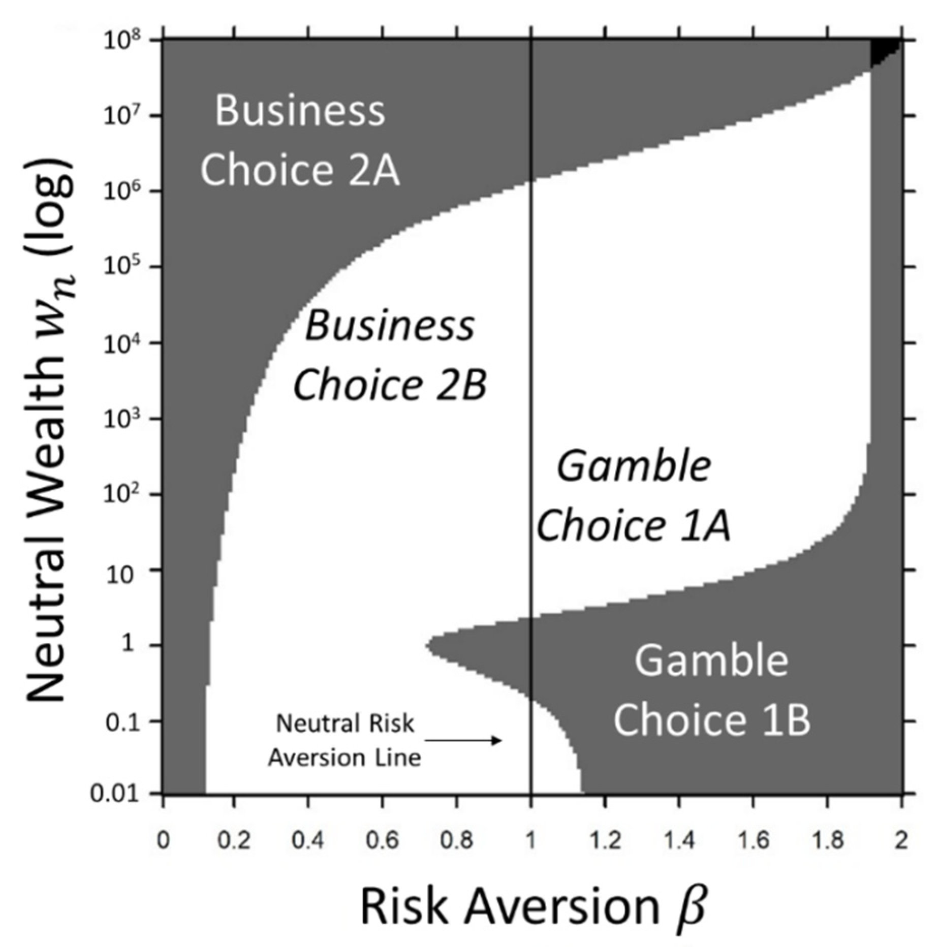
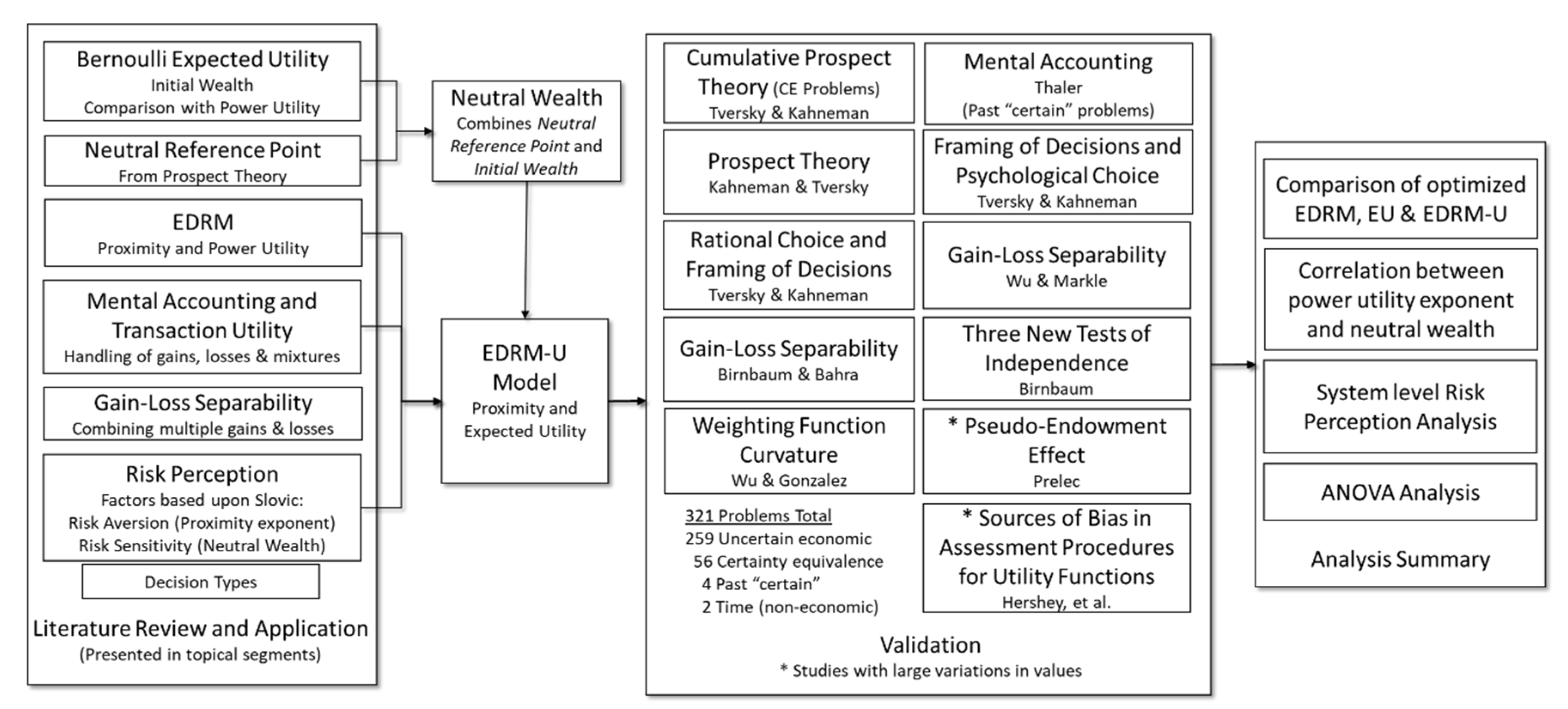
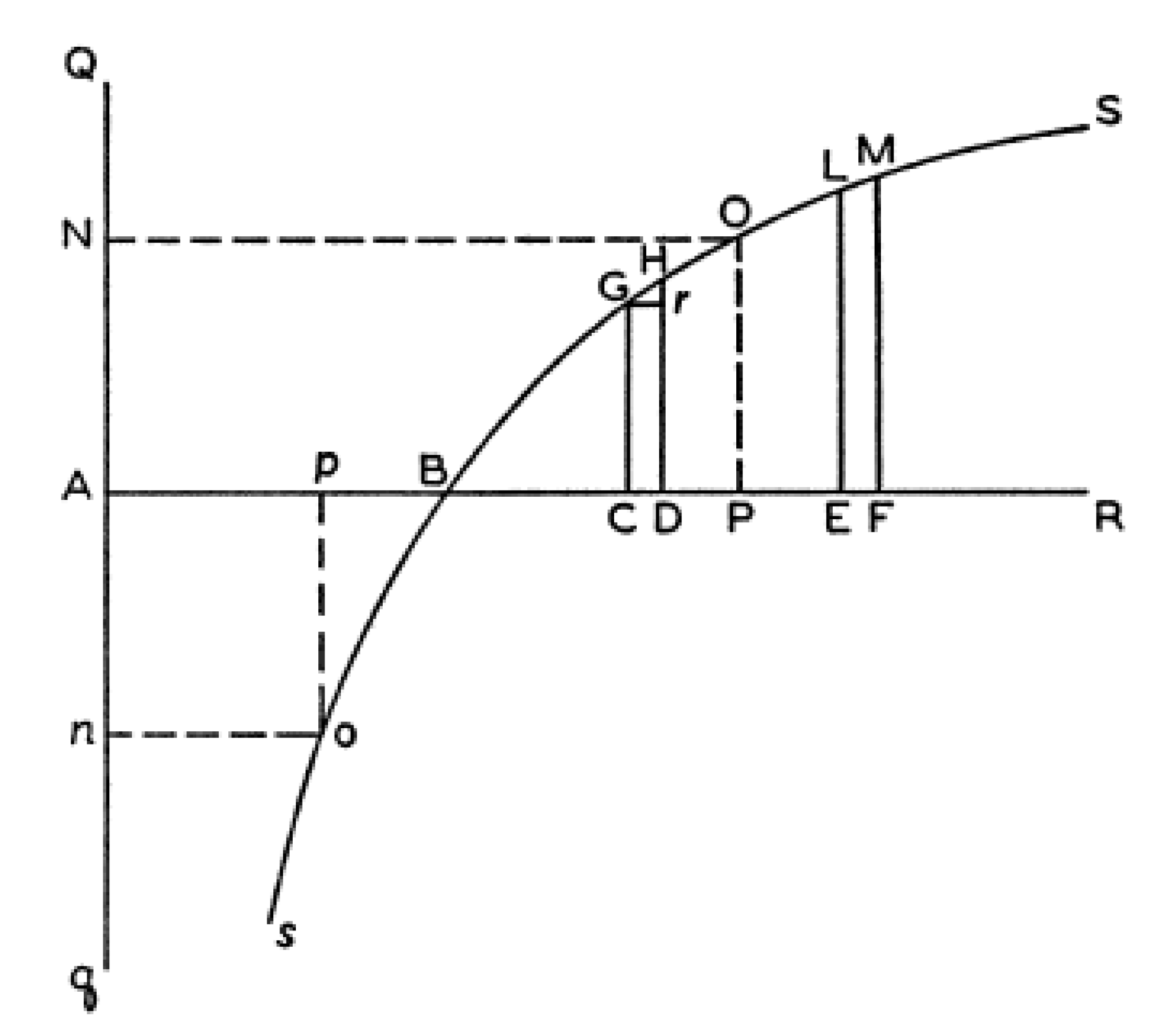
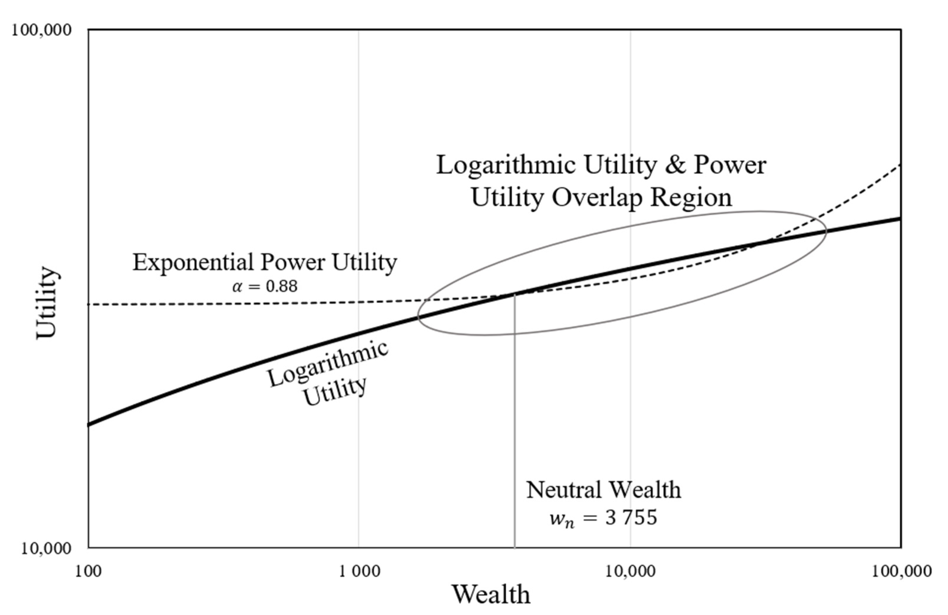
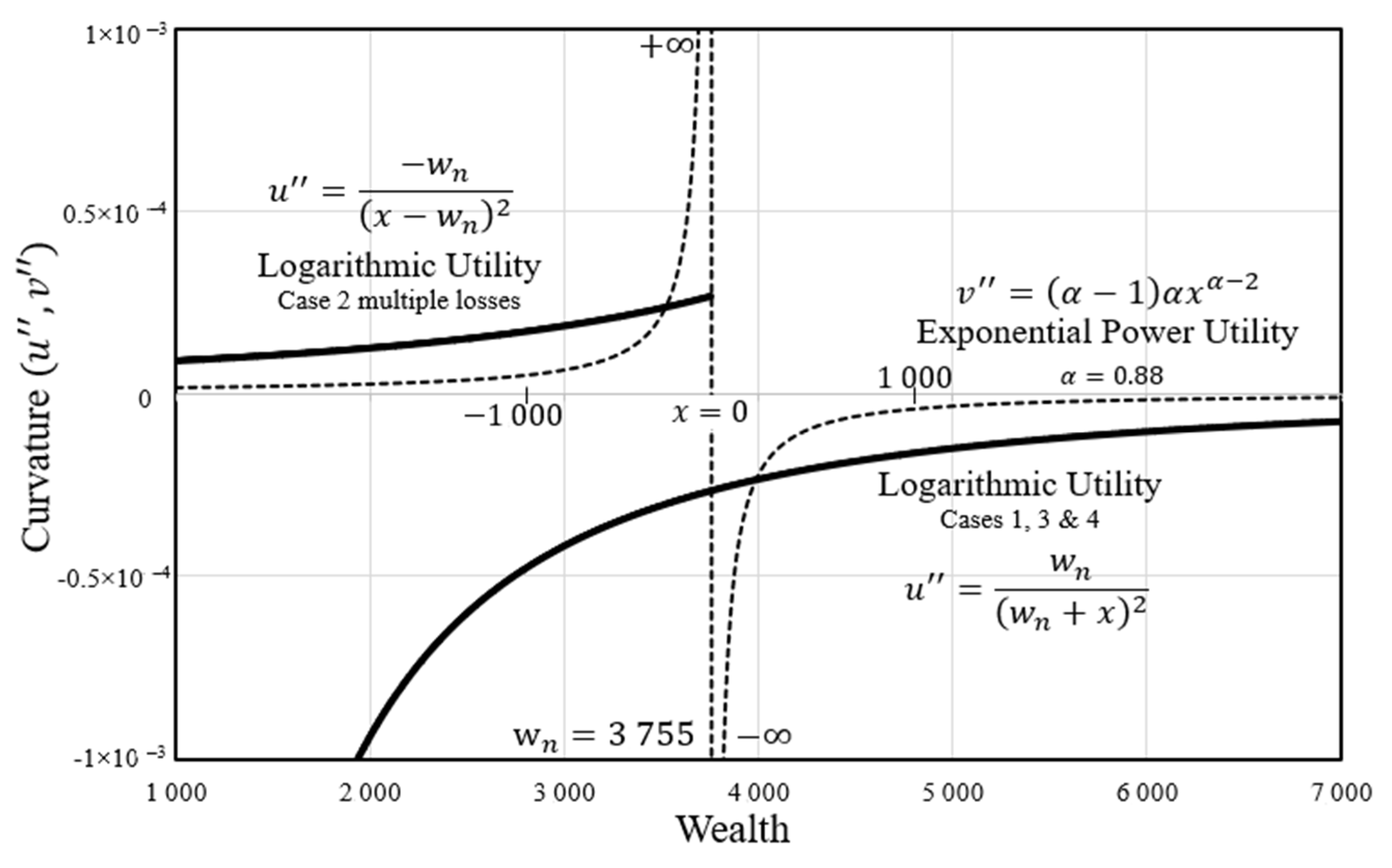
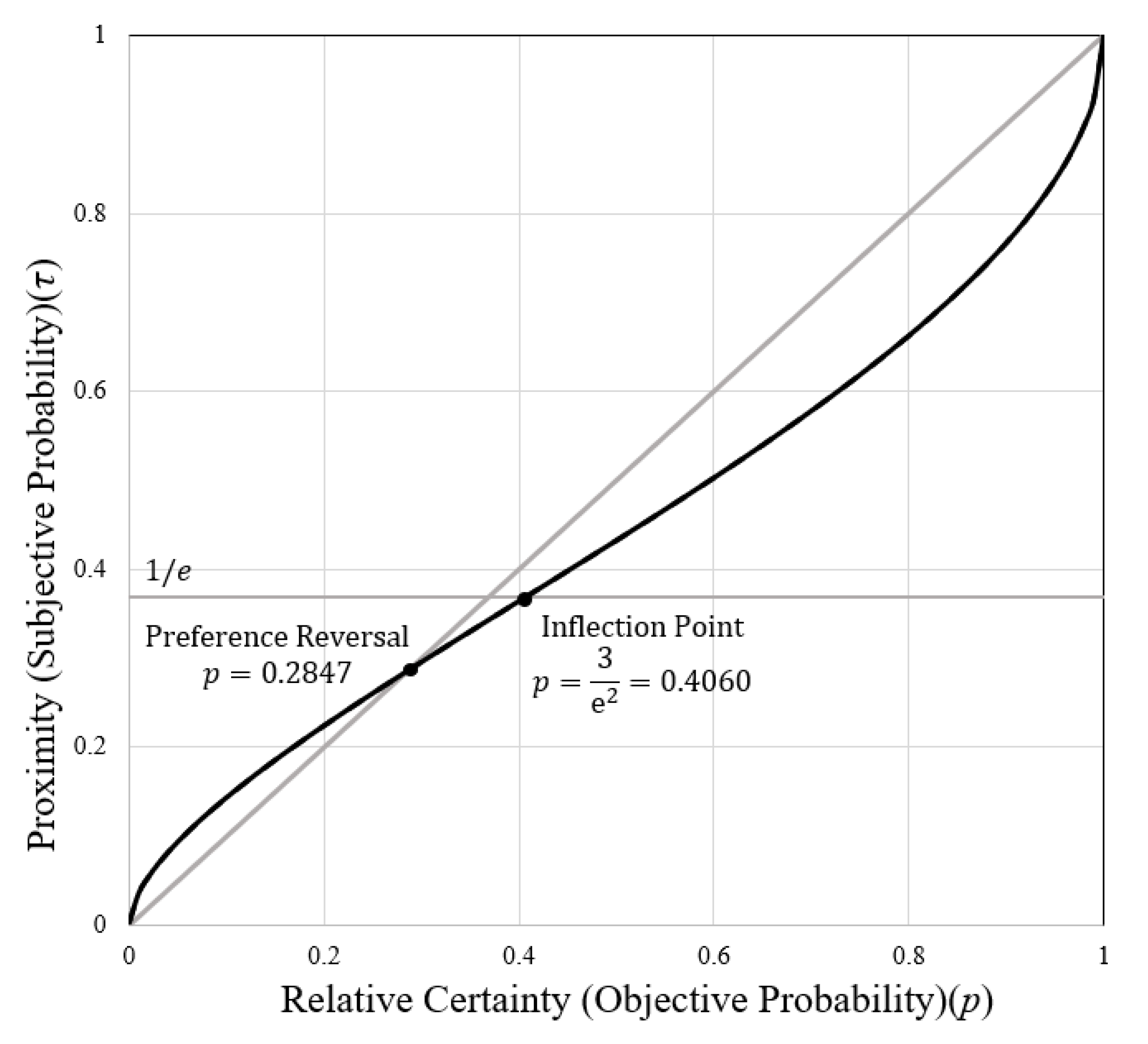
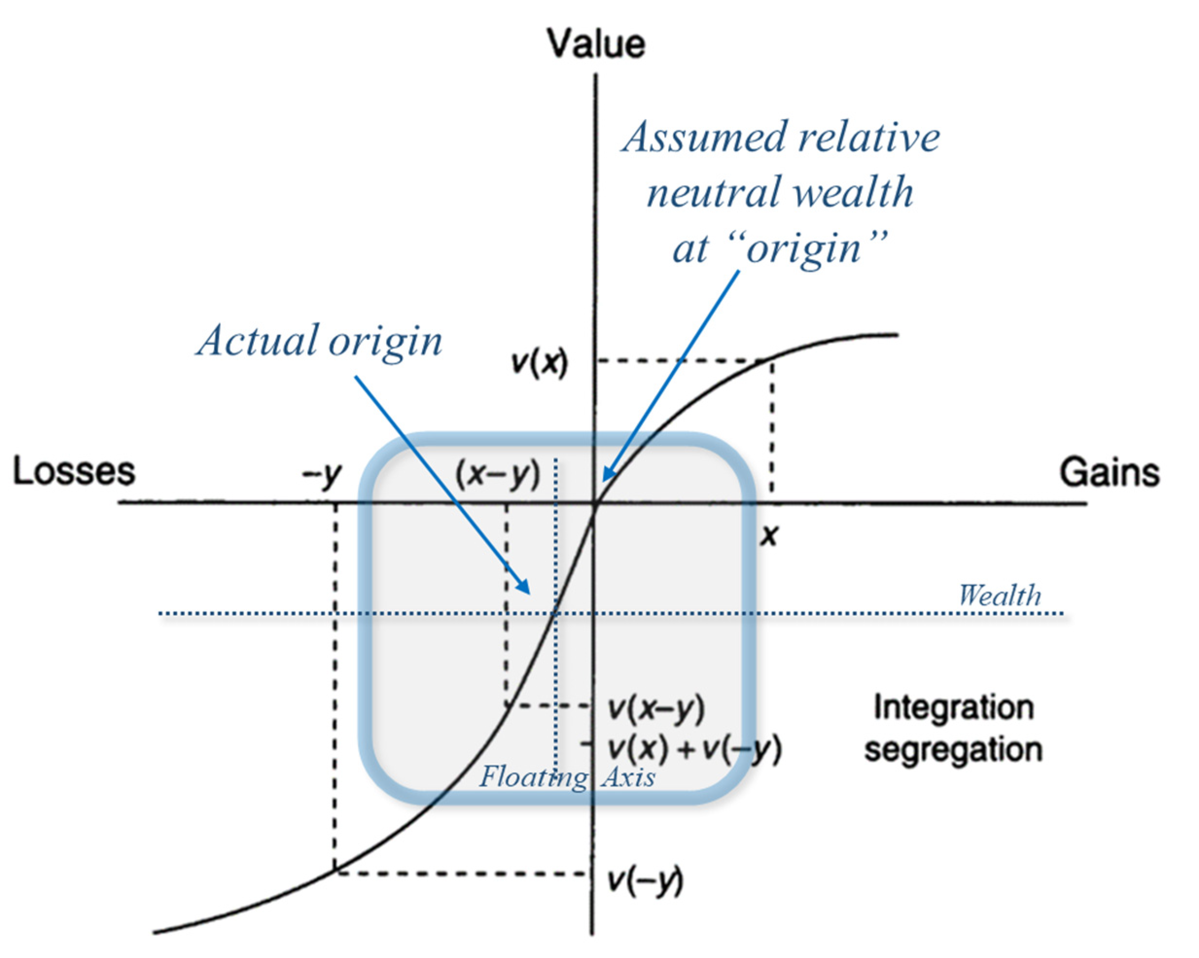
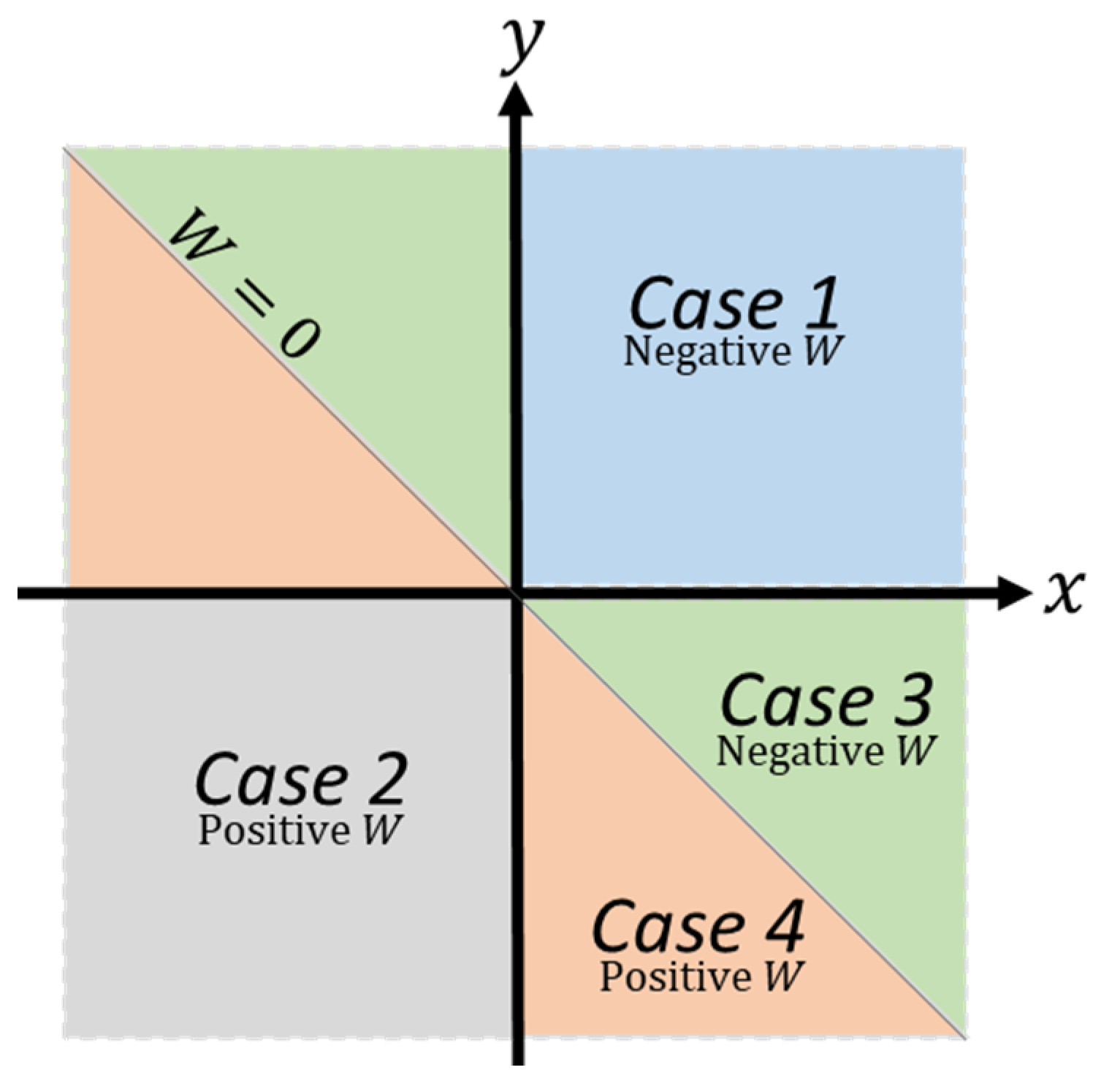
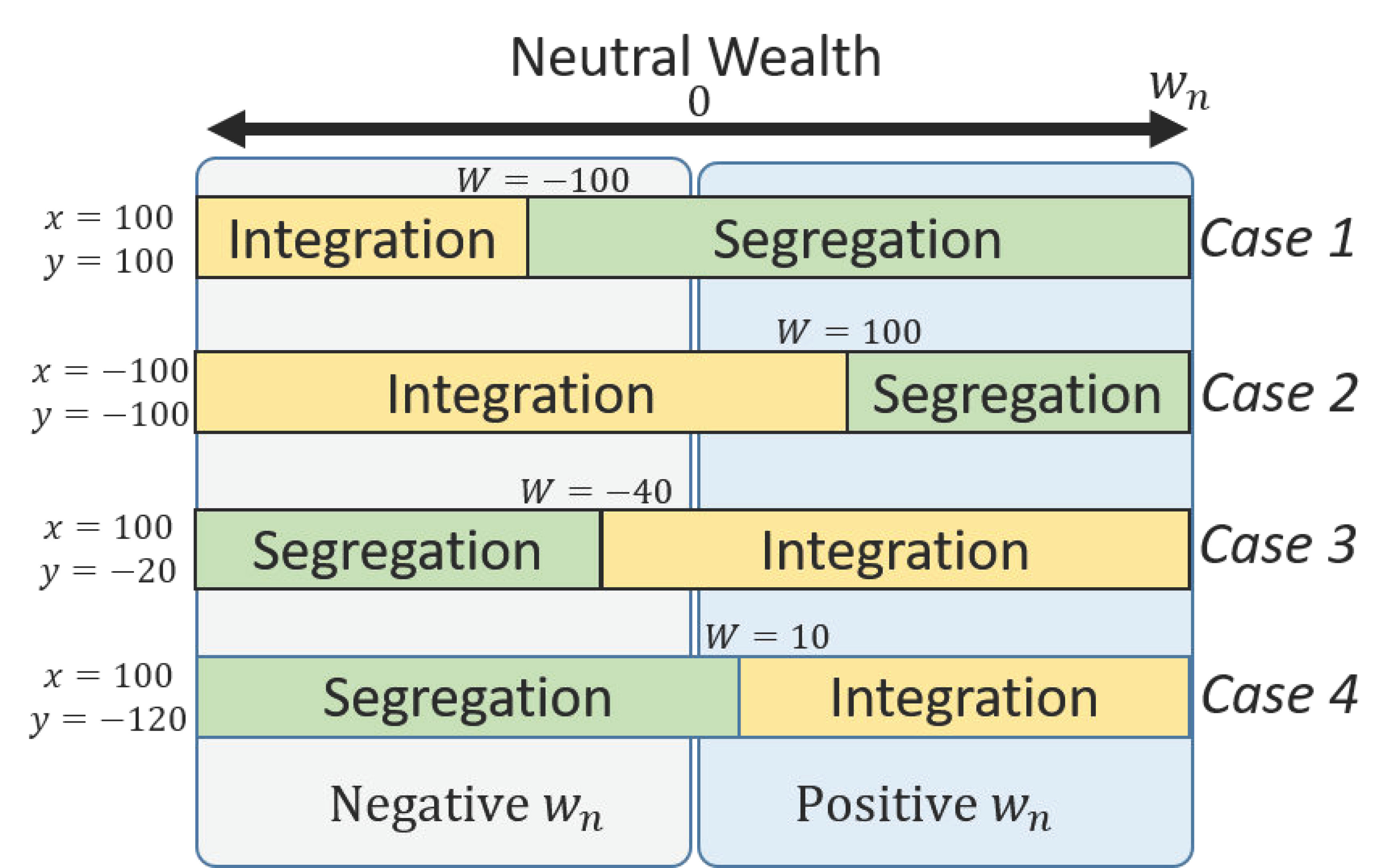
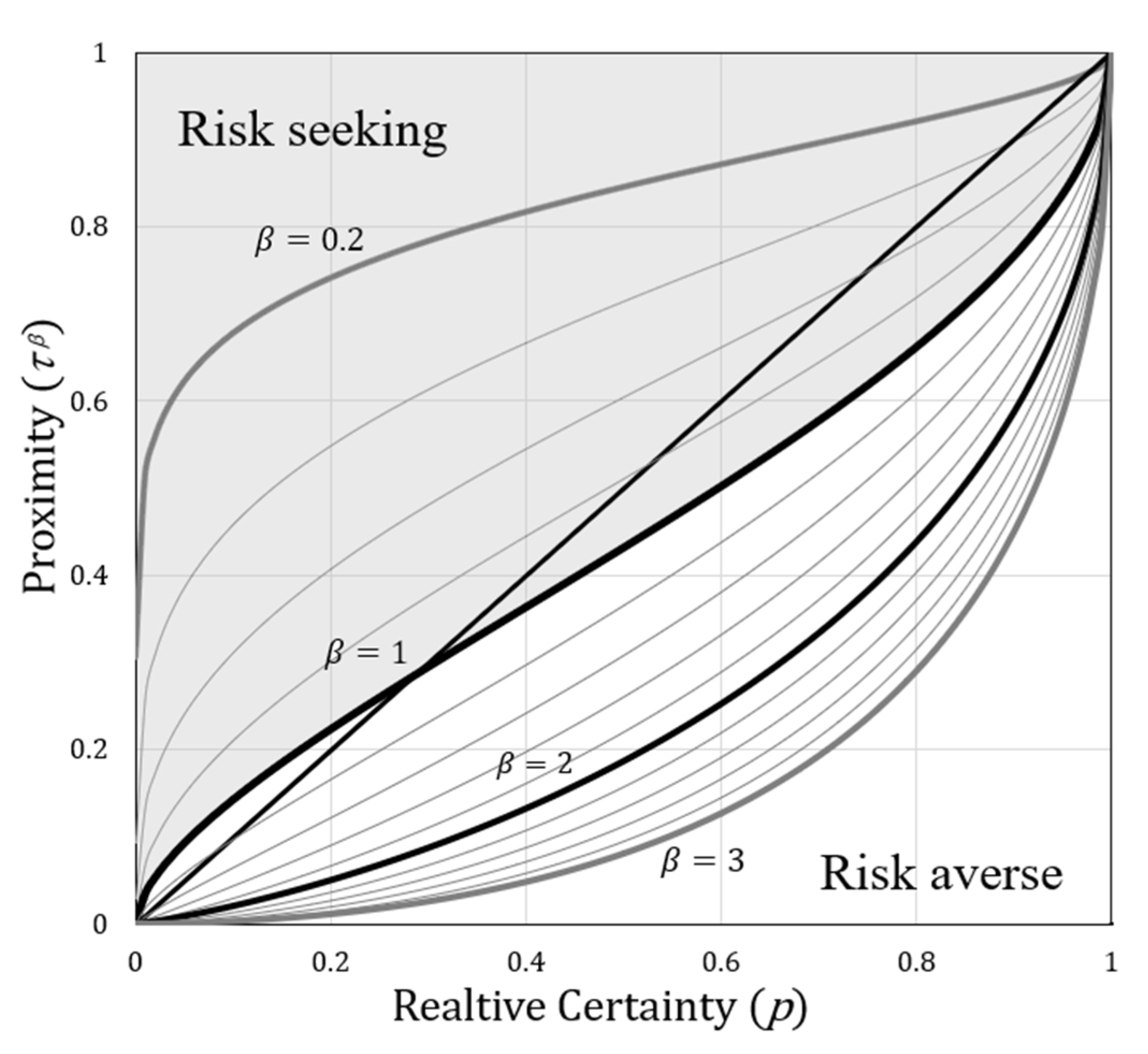
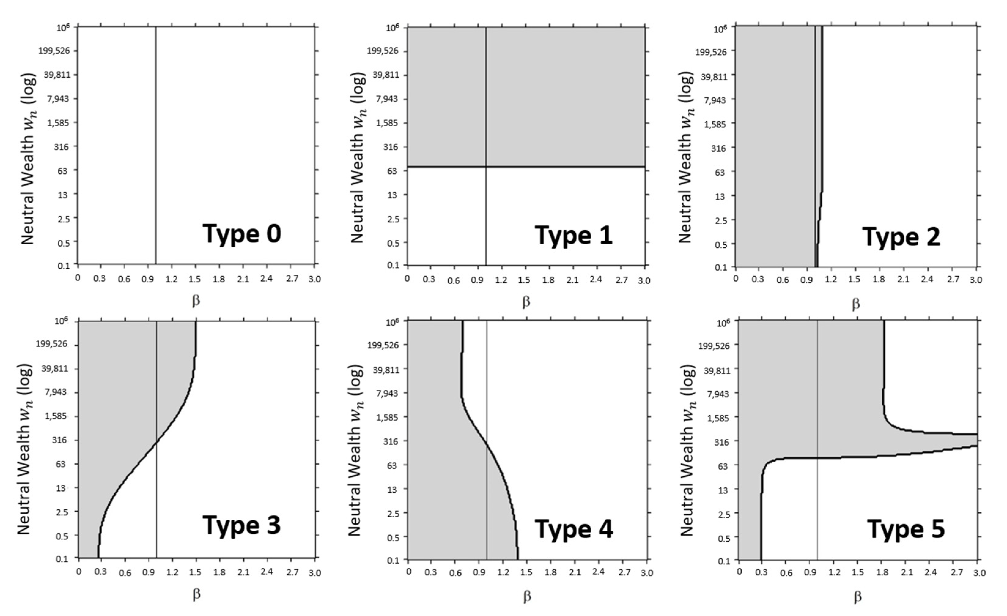
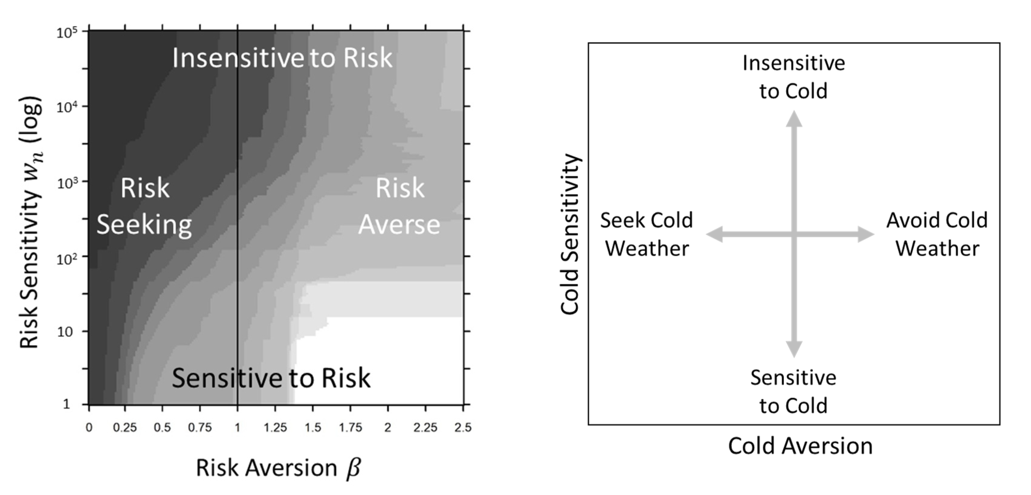
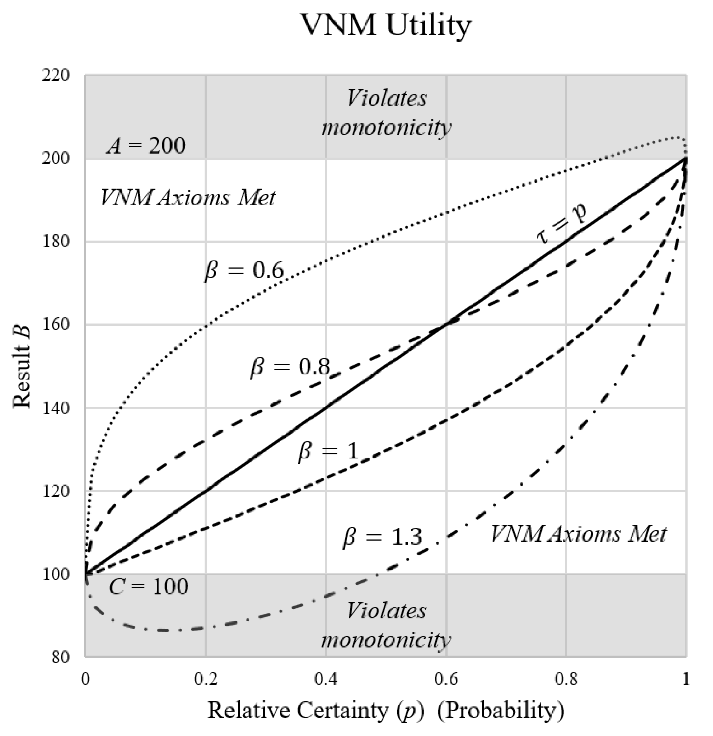
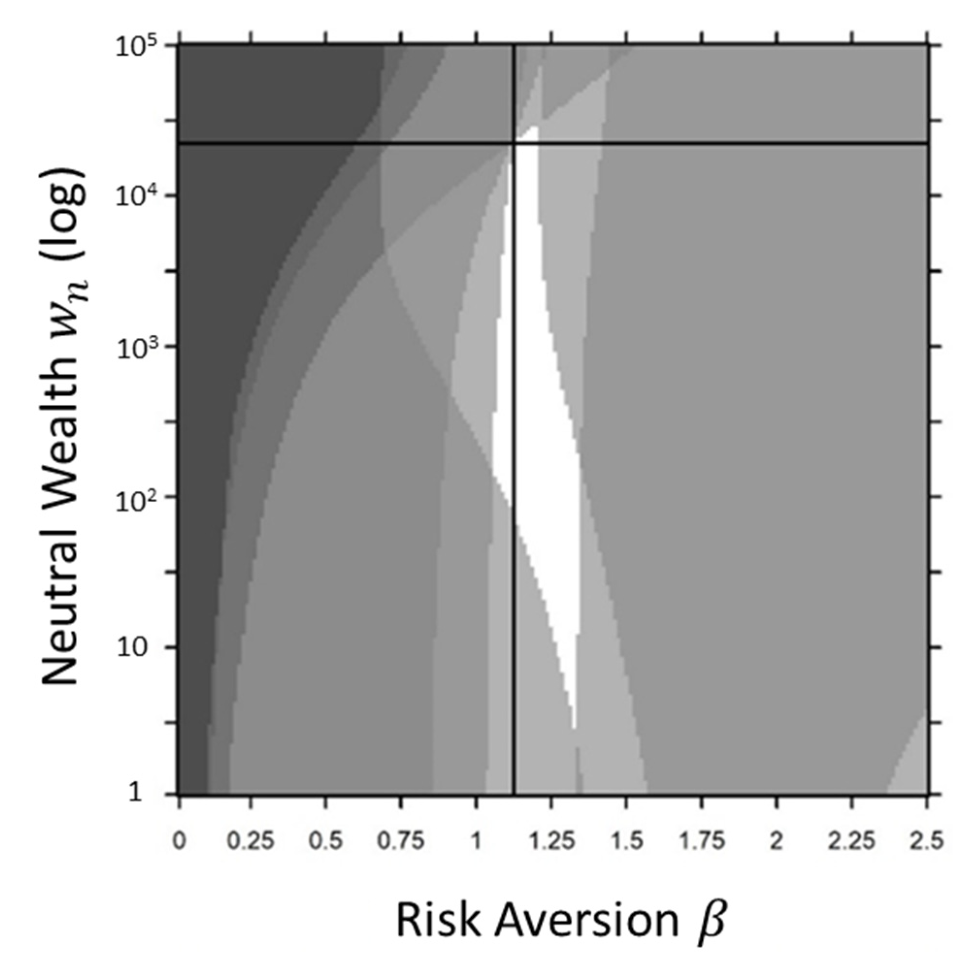
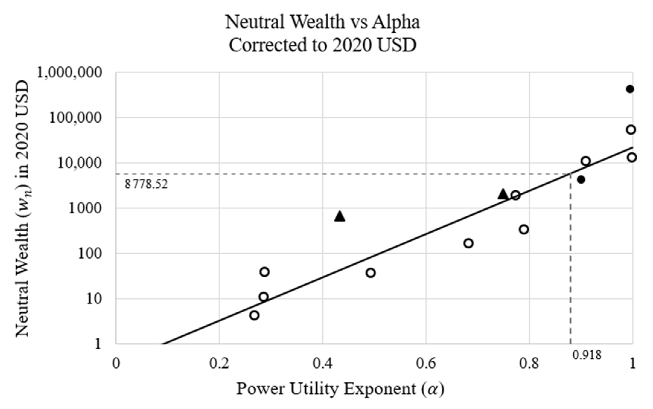
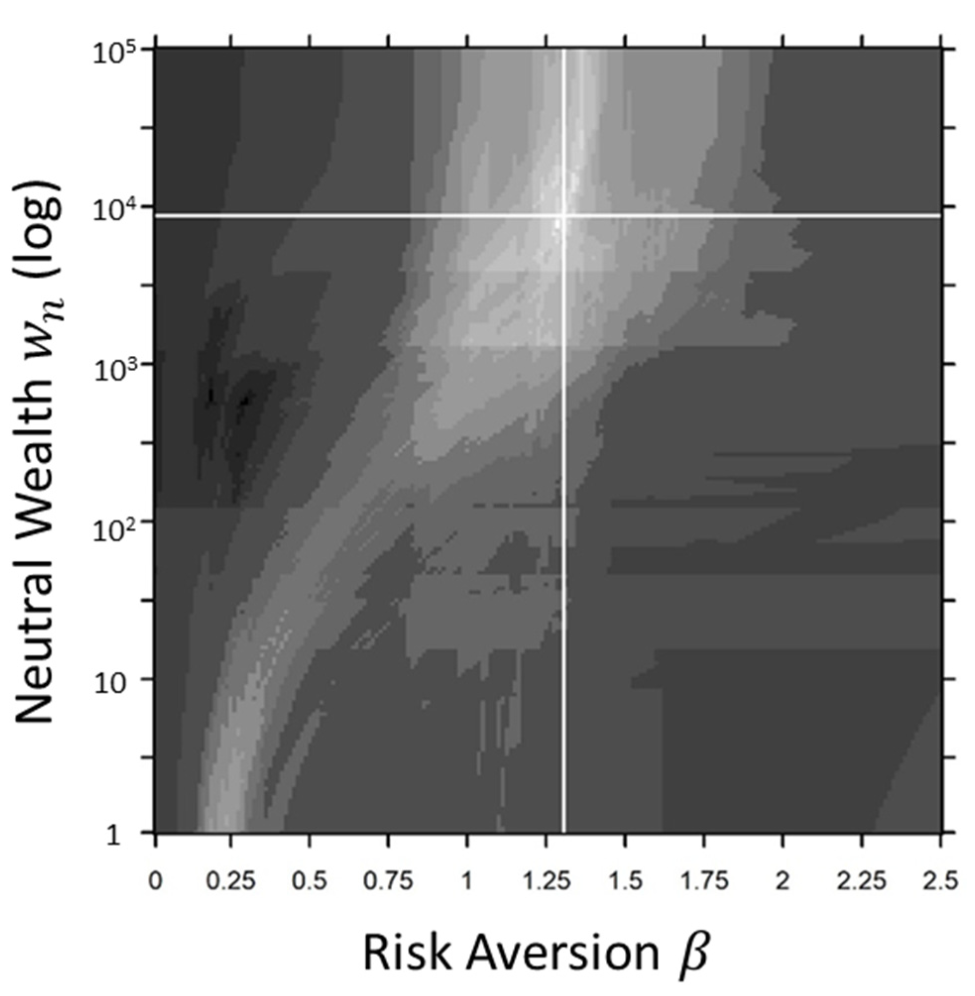
Table 1.
Comparison of EDRM, EU, and EDRM-U. Expected utility is the accepted normative standard for most economic small and large economic decisions. EDRM uses power utility, which is generally used in economic behavior models, but only performs well over small ranges of values. EDRM-U advances EDRM by using logarithmic expected utility instead of exponential power utility. As a result, EDRM-U is a general model that predicts subject choice for small and large economic values.
| Positive Theory | Normative Theory | Combined |
|---|---|---|
| EDRM | EU | EDRM-U |
| Proximity (subj prob) | Objective Probability | Proximity (subj prob) |
| Power Utility | Logarithmic Utility | Logarithmic Utility |
Table 2.
Neutral wealth effect on segregation and integration based upon the crossover value, .
| Pure Gain or Loss (No Cancellation) | Mixed (Cancellation) | |
|---|---|---|
| Segregation (e.g., prefer many separate gifts) | wn > W | wn < W |
| Integration (e.g., prefer a single billing statement) | wn < W | wn > W |
Table 3.
Comparison of risk perception factors showing that those used in this research are consistent with the two factors identified in prior studies and are aligned with established theory.
Table 3.
Comparison of risk perception factors showing that those used in this research are consistent with the two factors identified in prior studies and are aligned with established theory.
| Economic Decision Theories | Dual Process Theory | Risk Perception | Risk Perception | Risk Perception |
|---|---|---|---|---|
| Stanovich, et al. 2011 | Slovic & Peters 2006 | Sjöberg 2000 | This Research | |
| Positive, behavioral | Type 1 (intuition) | Risk as feelings | Risk attitude | Risk aversion (proximity exponent) |
| Normative, expectation | Type 2 (deliberate) | Risk as analysis | Risk sensitivity | Risk sensitivity (neutral wealth) |
Table 4.
Decision type examples (see Figure 11).
Table 4.
Decision type examples (see Figure 11).
| Type | Risky Choice (Value, Probability) | Safer Choice (Value, Probability) | Problem Source |
|---|---|---|---|
| 0 | (96, 0.45; 4, 0.45; 2, 0.1) | (58, 0.45; 56, 0.45; 2, 0.1) | Birnbaum 3–12 |
| 1 | (96, 0.45; 4, 0.45; 2, 0.1) | (44, 45; 40, 0.45; 2, 0.1) | Birnbaum 1–12 |
| 2 | (98, 0.85; 96; 0.05; 11, 0.1) | (99, 0.9; 14, 0.05; 12, 0.05) | Birnbaum 4–5 |
| 3 | (5000, 0.001) or (−5) | (5) or (−5000, 0.001) | Prospect Theory 14 or 14′ |
| 4 | (10,000, 0.01; 2000, 0.04) | (7000, 0.05)2 | Prelec 3AB |
| 5 | (1200, 0.3; −200, 0.7) | (400, 0.7; −800 0.3) | Wu-Markle 23 Mixed |
Table 5.
Description of analyses.
| Number matching | Number of binary matches and number of problems (used for optimization) |
| Binomial Prob (>50%) | Binomial probability of result being >50% (same as ratio) |
| Binomial p-Value | Resulting binomial p-value, values are acceptable |
| Matching Std dev () | Standard deviation of % difference of matches only (used for optimization) |
| All % Coeff of Det ( | Coefficient of determination between all actual and calculated percentages |
| All % Spearman rank () | Nonparametric rank test between all actual and calculated percentages |
Table 6.
EDRM versus EDRM-U: cumulative Prospect Theory.
| Unit: 1991 USD | EDRM | EDRM Optimal | EDRM-U | EDRM-U Optimal |
|---|---|---|---|---|
| Power utility exp () | 1 | 1 | ||
| Risk aversion () | 1 | 0.9473 | 1 | 0.9473 |
| Neutral Wealth () $ | ||||
| All Coeff of Det ( | 0.9971 | 0.9973 | 0.9971 | 0.9973 |
| All Spearman rank () | 0.9983 | 0.9985 | 0.9983 | 0.9985 |
Table 7.
EDRM-U optimized results for Thaler mental accounting (four observations).
| Unit: 1982 USD | ||||||||||
|---|---|---|---|---|---|---|---|---|---|---|
| Problem (Values Only) | EDRM-U | Calc% | Actual% | Diff | Match | |||||
| Outcome A | Outcome B | A | B | A | B | Y/N | ||||
| 1 | (50, 25) | (75) | 55.08 | 46.00 | 82 | 18 | 78 | 22 | −4.2 | Yes |
| 2 | (−100, −50) | (−150) | −89.96 | −69.70 | 10 | 90 | 18 | 83 | 7.8 | Yes |
| 3 | (−20, 100) | (80) | 29.75 | 47.98 | 30 | 70 | 27 | 73 | −3.0 | Yes |
| 4 | (25, −200) | (−175) | −501.83 | −512.88 | 66 | 34 | 77 | 23 | 10.7 | Yes |
Table 8.
EDRM versus EDRM-U: Thaler mental accounting.
| Unit: 1983 USD | EDRM Uncorrected | EDRM Optimal | EDRM-U Optimal |
|---|---|---|---|
| Power utility exp () | 0.88 | 0.688 | |
| Neutral Wealth () $ | 50.61 | ||
| Number matching | 4/4 | 4/4 | 4/4 |
| Binomial Prob (>50%) | 1 | 1 | 1 |
| Binomial p-Value | 0.125 | 0.125 | 0.125 |
| Matching Std dev () | 13.297 | 6.476 | 7.539 |
| All % Coeff of Det ( | 0.962 | 0.960 | 0.948 |
| All % Spearman rank () | 1 | 1 | 1 |
Table 9.
EDRM versus EDRM-U: Prospect Theory.
| Unit: 1978 Israeli Pound | EDRM Uncorrected | EDRM Optimal | EU Optimal | EDRM-U at | EDRM-U Optimal | |
|---|---|---|---|---|---|---|
| Power utility exp () | 0.88 | 0.87 | 0.853 | |||
| Risk aversion () | 1 | 1 | 0.9775 | 1 | 0.894 | |
| Neutral Wealth () I£ | 6750 | 3755 | ||||
| Number matching | 19/19 | 19/19 | 19/19 | 12/19 | 19/19 | 19/19 |
| Binomial Prob (>50%) | 1 | 1 | 1 | 0.632 | 1 | 1 |
| Binomial p-Value | 3.8 × 10⁻⁶ | 3.8 × 10⁻⁶ | 3.8 × 10⁻⁶ | 0.359 | 3.8 × 10⁻⁶ | 3.8 × 10⁻⁶ |
| Matching Std dev () | 10.868 | 10.825 | 10.821 | 10.844 | 9.903 | 9.642 |
| All % Coeff of Det ( | 0.859 | 0.859 | 0.859 | 0.519 | 0.882 | 0.888 |
| All % Spearman rank () | 0.697 | 0.701 | 0.701 | 0.645 | 0.705 | 0.699 |
Table 10.
EDRM versus EDRM-U: framing of decisions.
| Unit: 1980 USD | EDRM Uncorrected | EDRM | EDRM Optimal | EU Optimal | EDRM-U | EDRM-U Optimal |
|---|---|---|---|---|---|---|
| Power utility exp () | 0.88 | 0.65 | 0.65 | |||
| Risk aversion () | 1 | 1 | 1 | 1 | 0.668 | |
| Neutral Wealth () $ | 17.8 | 0.315 | ||||
| Number matching | 8/8 | 8/8 | 8/8 | 7/8 | 8/8 | 8/8 |
| Binomial Prob (>50%) | 1 | 1 | 1 | 0.875 | 1 | 1 |
| Binomial p-Value | 0.008 | 0.008 | 0.008 | 0.070 | 0.008 | 0.008 |
| Matching Std dev () | 8.757 | 6.023 | 6.023 | 8.613 | 7.810 | 6.312 |
| All % Coeff of Det ( | 0.945 | 0.968 | 0.968 | 0.960 | 0.958 | 0.965 |
| All % Spearman rank () | 0.850 | 0.850 | 0.850 | 0.850 | 0.850 | 0.850 |
Table 11.
EDRM optimized results for rational choice problem 1 (percent diff.).
| Unit: Years | EDRM | EDRM-U | EDRM-U | ||
|---|---|---|---|---|---|
| Problem (Years, Probability) | |||||
| A-Surgery | B-Radiation | Act%-Calc% | Act%-Calc% | Act%-Calc% | |
| 1a (1 year) | (1, 0.68; 5, 0.34; 1, 0.9) | (1, 0.77; 5, 0.22) | 6% | 11% | 20% |
| 1b | (−1, 0.32; −5, 0.66) | (−1, 0.23; −5, 0.78) | 1% | 1% | 1% |
| 1a (5 years) | (1, 0.68; 5, 0.34; 5, 0.9) | (1, 0.77; 5, 0.22) | −13% | −17% | 0% |
| 1b | (−1, 0.32; −5, 0.66) | (−1, 0.23; −5, 0.78) | 1% | 1% | 1% |
Table 12.
EDRM versus EDRM-U: rational choice and the framing of decisions.
| Unit: 1985 USD | EDRM Uncorrected | EDRM | EDRM Optimal | EU Optimal | EDRM-U | EDRM-U Optimal |
|---|---|---|---|---|---|---|
| Power utility exp () | 0.88 | 0.649 | 0.328 | |||
| Risk aversion () | 1 | 1 | 0.503 | 1 | 1.420 | |
| Neutral Wealth () $ | 11.885 | |||||
| Number matching | 12/14 | 14/14 | 14/14 | 11/14 | 14/14 | 14/14 |
| Binomial Prob (>50%) | 0.857 | 1 | 1 | 0.786 | 1 | 1 |
| Binomial p-Value | 0.013 | 1.2 × 10⁻⁴ | 1.2 × 10⁻⁴ | 0.057 | 1.2 × 10⁻⁴ | 1.2 × 10⁻⁴ |
| Matching Std dev () | 7.911 | 8.410 | 8.334 | 11.124 | 10.110 | 8.720 |
| All % Coeff of Det ( | 0.793 | 0.910 | 0.911 | 0.883 | 0.899 | 0.898 |
| All % Spearman rank () | 0.864 | 0.917 | 0.917 | 0.900 | 0.917 | 0.917 |
Table 13.
EDRM versus EDRM-U: Wu Markle gains only.
| Unit: 2006 USD | EDRM Uncorrected | EDRM | EDRM Optimal | EU Optimal | EDRM-U | EDRM-U Optimal |
|---|---|---|---|---|---|---|
| Power utility exp () | 0.88 | 0.557 | 0.557 | |||
| Risk aversion () | 1 | 1 | 1 | 1 | 1.530 | |
| Neutral Wealth () $ | 625 | 7599 | ||||
| Number matching | 23/34 | 31/34 | 31/34 | 31/34 | 29/34 | 31/34 |
| Binomial Prob (>50%) | 0.676 | 0.912 | 0.912 | 0.912 | 0.853 | 0.912 |
| Binomial p-Value | 0.058 | 7.7 × 10⁻⁷ | 7.7 × 10⁻⁷ | 7.7 × 10⁻⁷ | 3.9 × 10⁻⁵ | 7.7 × 10⁻⁷ |
| Matching Std dev () | 7.884 | 11.297 | 11.297 | 12.236 | 12.126 | 11.202 |
| All % Coeff of Det ( | 0.514 | 0.565 | 0.565 | 0.671 | 0.467 | 0.618 |
| All % Spearman rank () | 0.725 | 0.776 | 0.776 | 0.766 | 0.688 | 0.780 |
Table 14.
EDRM versus EDRM-U: Wu Markle losses only.
| Unit: 2006 USD | EDRM Uncorrected | EDRM | EDRM Optimal | EU Optimal | EDRM-U | EDRM-U Optimal |
|---|---|---|---|---|---|---|
| Power utility exp () | 0.88 | 0.581 | 1 | |||
| Risk aversion () | 1 | 1 | 1.721 | 1 | 1.721 | |
| Neutral Wealth () $ | 51.5 | |||||
| Number matching | 19/34 | 28/34 | 28/34 | 20/34 | 21/34 | 28/34 |
| Binomial Prob (>50%) | 0.559 | 0.824 | 0.824 | 0.588 | 0.618 | 0.824 |
| Binomial p-Value | 0.608 | 2.0 × 10⁻⁴ | 2.0 × 10⁻⁴ | 0.392 | 0.230 | 2.0 × 10⁻⁴ |
| Matching Std dev () | 10.205 | 12.237 | 12.237 | 8.976 | 10.086 | 12.237 |
| All % Coeff of Det ( | 0.475 | 0.505 | 0.505 | 0.084 | 0.042 | 0.505 |
| All % Spearman rank () | 0.816 | 0.678 | 0.678 | 0.241 | 0.354 | 0.678 |
Table 15.
EDRM versus EDRM-U: Wu Markle mixed gains and losses.
| Unit: 2006 USD | EDRM Uncorrected | EDRM | EDRM Optimal | EU Optimal | EDRM-U | EDRM-U Optimal |
|---|---|---|---|---|---|---|
| Power utility exp () | 0.88 | 0.8205 | 1 | |||
| Risk aversion () | 1 | 1 | 1.208 | 1 | 1.39 | |
| Neutral Wealth () $ | 12975 | 4375 | ||||
| Number matching | 28/34 | 28/34 | 28/34 | 20/34 | 28/34 | 30/34 |
| Binomial Prob (>50%) | 0.824 | 0.824 | 0.824 | 0.588 | 0.824 | 0.882 |
| Binomial p-Value | 2.0 × 10⁻⁴ | 2.0 × 10⁻⁴ | 2.0 × 10⁻⁴ | 0.392 | 2.0 × 10⁻⁴ | 2.0 × 10⁻⁶ |
| Matching Std dev () | 8.818 | 8.603 | 8.361 | 12.919 | 9.309 | 8.557 |
| All % Coeff of Det ( | 0.352 | 0.380 | 0.384 | 0.135 | 0.305 | 0.456 |
| All % Spearman rank () | 0.703 | 0.687 | 0.697 | 3.4 × 10⁻¹¹ | 0.725 | 0.624 |
Table 16.
EDRM versus EDRM-U: Birnbaum and Bahra gain loss separability.
| Unit: 2004 USD | EDRM Uncorrected | EDRM | EDRM Optimal | EU Optimal | EDRM-U | EDRM-U Optimal |
|---|---|---|---|---|---|---|
| Power utility exp () | 0.88 | 0.898 | 0.848 | |||
| Risk aversion () | 1 | 1 | 0.846 | 1 | 0.968 | |
| Neutral Wealth () $ | 993.27 | 995.75 | ||||
| Number matching | 14/18 | 14/18 | 14/18 | 13/18 | 17/18 | 17/18 |
| Binomial Prob (>50%) | 0.778 | 0.778 | 0.778 | 0.722 | 0.944 | 0.944 |
| Binomial p-Value | 0.031 | 0.031 | 0.031 | 0.096 | 1.5 × −4 | 1.5 × 10⁻⁴ |
| Matching Std dev () | 8.800 | 8.751 | 7.187 | 12.981 | 8.855 | 8.773 |
| All % Coeff of Det ( | 0.615 | 0.619 | 0.685 | 0.313 | 0.678 | 0.685 |
| All % Spearman rank () | 0.800 | 0.800 | 0.860 | 0.317 | 0.800 | 0.804 |
Table 17.
EDRM versus EDRM-U: Birnbaum.
| Unit: 2003 USD | EDRM Uncorrected | EDRM | EDRM Optimal | EU Optimal | EDRM-U | EDRM-U Optimal |
|---|---|---|---|---|---|---|
| Power utility exp () | 0.88 | 0.5 | 0.5 | |||
| Risk aversion () | 1 | 1 | 0.93 | 1 | 1.001 | |
| Neutral Wealth () $ | 22.75 | 22.75 | ||||
| Number matching | 11/21 | 19/21 | 19/21 | 16/21 | 18/21 | 18/21 |
| Binomial Prob (>50%) | 0.524 | 0.905 | 0.905 | 0.762 | 0.857 | 0.857 |
| Binomial P-Value | 1 | 2.2 × 10⁻⁴ | 2.2 × 10⁻⁴ | 0.027 | 1.5 × 10⁻³ | 1.5 × 10⁻³ |
| Matching Std dev () | 8.257 | 7.290 | 6.975 | 7.376 | 5.841 | 5.850 |
| All % Coeff of Det ( | 0.244 | 0.746 | 0.731 | 0.571 | 0.712 | 0.713 |
| All % Spearman rank () | 0.250 | 0.880 | 0.885 | 0.719 | 0.878 | 0.878 |
Table 18.
EDRM versus EDRM-U: Wu and Gonzalez.
| Unit: 1995 USD | EDRM Uncorrected | EDRM | EDRM Optimal | EU Optimal | EDRM-U | EDRM-U Optimal |
|---|---|---|---|---|---|---|
| Power utility exp () | 0.88 | 0.5885 | 0.387 | |||
| Risk aversion () | 1 | 1 | 1.220 | 1 | 1.221 | |
| Neutral Wealth () $ | 99 | 23.4 | ||||
| Number matching | 26/40 | 30/40 | 33/40 | 18/40 | 29/40 | 34/40 |
| Binomial Prob (>50%) | 0.650 | 0.750 | 0.825 | 0.450 | 0.725 | 0.850 |
| Binomial P-Value | 0.081 | 2.2 × 10⁻³ | 4.2 × 10⁻⁵ | 0.636 | 6.4 × 10⁻³ | 8.4 × 10⁻⁶ |
| Matching Std dev () | 5.998 | 7.191 | 9.031 | 8.290 | 7.110 | 7.990 |
| All % Coeff of Det ( | 0.473 | 0.482 | 0.393 | 1.0 × 10⁻⁵ | 0.499 | 0.474 |
| All % Spearman rank () | 0.449 | 0.484 | 0.645 | 0.114 | 0.522 | 0.712 |
Table 19.
EDRM versus EDRM-U: Prelec.
| Unit: 1989 USD | EDRM Uncorrected | EDRM | EDRM Optimal | EU Optimal | EDRM-U | EDRM-U Optimal |
|---|---|---|---|---|---|---|
| Power utility exp () | 0.88 | 0.543 | 0.467 | |||
| Risk aversion () | 1 | 1 | 1.268 | 1 | 1.12 | |
| Neutral Wealth () $ | 4765 | 22170 | ||||
| Number matching | 5/9 | 7/9 | 9/9 | 7/9 | 8/9 | 9/9 |
| Binomial Prob (>50%) | 0.556 | 0.778 | 1 | 0.778 | 0.889 | 1 |
| Binomial P-Value | 1 | 0.180 | 3.9 × 10⁻³ | 0.180 | 0.039 | 3.9 × 10⁻³ |
| Matching Std dev () | 6.940 | 7.575 | 16.201 | 12.617 | 9.160 | 7.245 |
| All % Coeff of Det ( | 0.320 | 0.720 | 0.558 | 0.124 | 0.803 | 0.924 |
| All % Spearman rank () | 0.433 | 0.850 | 0.700 | 0.333 | 0.900 | 0.983 |
Table 20.
EDRM versus EDRM-U: Hershey losses.
| Unit: 1980 USD | EDRM Uncorrected | EDRM | EDRM Optimal | EU Optimal | EDRM-U | EDRM-U Optimal |
|---|---|---|---|---|---|---|
| Power utility exp () | 0.88 | 0.250 | 1 | |||
| Risk aversion () | 1 | 1 | 4.003 | 1 | 4.003 | |
| Neutral Wealth () $ | 0 | |||||
| Number matching | 6/10 | 10/10 | 10/10 | 10/10 | 10/10 | 10/10 |
| Binomial Prob (>50%) | 0.6 | 1 | 1 | 1 | 1 | 1 |
| Binomial P-Value | 0.705 | 2.0 × 10⁻³ | 2.0 × 10⁻³ | 2.0 × 10⁻³ | 2.0 × 10⁻³ | 2.0 × 10⁻³ |
| Matching Std dev () | 15.484 | 9.586 | 9.586 | 10.231 | 10.704 | 9.586 |
| All % Coeff of Det ( | 0.206 | 0.272 | 0.272 | 0.181 | 0.191 | 0.272 |
| All % Spearman rank () | 0.345 | 0.564 | 0.564 | 0.394 | 0.418 | 0.564 |
Table 21.
EDRM versus EDRM-U: Hershey gains.
| Unit: 1980 USD | EDRM Uncorrected | EDRM | EDRM Optimal | EU Optimal | EDRM-U | EDRM-U Optimal |
|---|---|---|---|---|---|---|
| Power utility exp () | 0.88 | 1 | 0.891 | |||
| Risk aversion () | 1 | 1 | 0.748 | 1 | 0.325 | |
| Neutral Wealth () $ | 274.25 | 1.494 | ||||
| Number matching | 12/18 | 13/18 | 13/18 | 9/18 | 18/18 | 18/18 |
| Binomial Prob (>50%) | 0.667 | 0.722 | 0.722 | 0.500 | 1 | 1 |
| Binomial P-Value | 0.238 | 0.096 | 0.096 | 1 | 7.6 × 10⁻⁶ | 7.6 × 10⁻⁶ |
| Matching Std dev () | 14.877 | 14.304 | 13.849 | 7.254 | 7.829 | 6.332 |
| All % Coeff of Det ( | 0.075 | 0.116 | 0.151 | 0.584 | 0.869 | 0.913 |
| All % Spearman rank () | −0.044 | −0.055 | −0.064 | 0.717 | 0.890 | 0.956 |
Table 22.
EDRM versus EDRM-U: combined weighted averages of results optimized by study.
| Weighted Averages | EDRM Uncorrected | EDRM | EDRM Optimal | EU Optimal | EDRM-U | EDRM-U Optimal |
|---|---|---|---|---|---|---|
| Number matching | 183/259 | 221/259 | 226/259 | 174/259 | 219/259 | 236/259 |
| Binomial Prob (>50%) | 0.707 | 0.853 | 0.873 | 0.672 | 0.846 | 0.911 |
| Matching Std dev () | 9.108 | 9.591 | 9.973 | 10.261 | 9.115 | 8.954 |
| All % Coeff of Det ( | 0.471 | 0.554 | 0.541 | 0.352 | 0.527 | 0.636 |
| All % Spearman rank () | 0.589 | 0.658 | 0.683 | 0.497 | 0.676 | 0.760 |
Table 23.
Risk perception analysis using optimized EDRM, EU, and EDRM-U (all as one group).
| Optimal EDRM | All | Gain Only | Loss Only | Mix Only |
|---|---|---|---|---|
| Power utility exp (α) | 0.7095 | |||
| Risk aversion () | 1.012 | 1.012 | 0.988 | 0.969 |
| Number matching | 202/259 | 120/154 | 52/61 | 33/44 |
| Optimal EU | ||||
| Initial wealth () $ | 24.90 | |||
| Number matching | 144/259 | 88/154 | 43/61 | 12/44 |
| Optimal EDRM-U | ||||
| ) $ | 8778.52 | |||
| Risk aversion () | 1.306 | 1.245 | 1.604 | 1.306 |
| Number matching | 209/259 | 120/154 | 52/61 | 39/44 |
Table 24.
EDRM versus EDRM-U ANOVA summary analysis.
| EDRM | EDRM-U | |||
|---|---|---|---|---|
| Actual-Calc % Diff (prob > F) | ||||
| Type (Gain, Loss, Mix) | 0.5160 | Not Significant | 0.9206 | Not Significant |
| Match (yes, no) | 0.1992 | Not Significant | 0.2364 | Not Significant |
| Interaction (Type and Match) | 0.0329 | Significant | 0.2785 | Not Significant |
| Magnitude (prob > F) (Corrected to 2020 USD) | ||||
| Act-Calc % Diff | 0.7101 | Not Significant | 0.4448 | Not Significant |
| Match (yes, no) | 0.9461 | Not Significant | 0.5930 | Not Significant |
| Interaction (% Diff and Match) | 0.0672 | Marginal | 0.6293 | Not Significant |
| Normality (p-value) | ||||
| Shapiro–Wilk | 8.21 × 10⁻⁴ | Not Normal6 | 0.6774 | Normal |
| Normality Plots | Normal, except at the lower extreme due to Hershey et al. gains (See Section 5.13.2). | Normal | ||
Publisher’s Note: MDPI stays neutral with regard to jurisdictional claims in published maps and institutional affiliations. |
© 2020 by the authors. Licensee MDPI, Basel, Switzerland. This article is an open access article distributed under the terms and conditions of the Creative Commons Attribution (CC BY) license (http://creativecommons.org/licenses/by/4.0/).
Share and Cite
MDPI and ACS Style
Monroe, T.; Beruvides, M.; Tercero-Gómez, V. Quantifying Risk Perception: The Entropy Decision Risk Model Utility (EDRM-U). Systems 2020, 8, 51. https://0-doi-org.brum.beds.ac.uk/10.3390/systems8040051
AMA Style
Monroe T, Beruvides M, Tercero-Gómez V. Quantifying Risk Perception: The Entropy Decision Risk Model Utility (EDRM-U). Systems. 2020; 8(4):51. https://0-doi-org.brum.beds.ac.uk/10.3390/systems8040051
Chicago/Turabian StyleMonroe, Thomas, Mario Beruvides, and Víctor Tercero-Gómez. 2020. "Quantifying Risk Perception: The Entropy Decision Risk Model Utility (EDRM-U)" Systems 8, no. 4: 51. https://0-doi-org.brum.beds.ac.uk/10.3390/systems8040051
Note that from the first issue of 2016, this journal uses article numbers instead of page numbers. See further details here.