
How Perspectives of a System Change Based on Exposure to Positive or Negative Evidence


1
Department of Computer Science and Software Engineering, Miami University, Oxford, OH 45056, USA
2
Department of Instructional Design and Technology, University of Memphis, Memphis, TN 38152, USA
*
Author to whom correspondence should be addressed.
Systems 2021, 9(2), 23; https://0-doi-org.brum.beds.ac.uk/10.3390/systems9020023
Submission received: 15 March 2021
/
Revised: 29 March 2021
/
Accepted: 1 April 2021
/
Published: 5 April 2021
(This article belongs to the Section Complex Systems)
Abstract
:The system that shapes a problem can be represented using a map, in which relevant constructs are listed as nodes, and salient interrelationships are provided as directed edges which track the direction of causation. Such representations are particularly useful to address complex problems which are multi-factorial and may involve structures such as loops, in contrast with simple problems which may have a clear root cause and a short chain of causes-and-effects. Although students are often evaluated based on either simple problems or simplified situations (e.g., true/false, multiple choice), they need systems thinking skills to eventually deal with complex, open-ended problems in their professional lives. A starting point is thus to construct a representation of the problem space, such as a causal map, and then to identify and contrast solutions by navigating this map. The initial step of abstracting a system into a map is challenging for students: unlike seasoned experts, they lack a detailed understanding of the application domain, and hence struggle in capturing its key concepts and interrelationships. Case libraries can remedy this disadvantage, as they can transfer the knowledge of experts to novices. However, the content of the cases can impact the perspectives of students. For example, their understanding of a system (as reflected in a map) may differ when they are exposed to case studies depicting successful or failed interventions in a system. Previous studies have abundantly documented that cases can support students, using a variety of metrics such as test scores. In the present study, we examine the ways in which the representation of a system (captured as a causal map) changes as a function of exposure to certain types of evidence. Our experiments across three cohorts at two institutions show that providing students with cases tends to broaden their coverage of the problem space, but the knowledge afforded by the cases is integrated in the students’ maps differently depending on the type of case, as well as the cohort of students.
1. Introduction
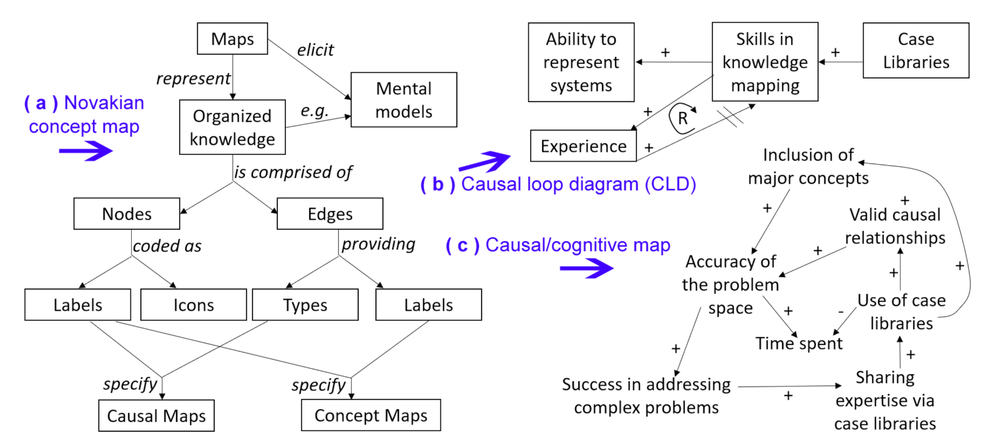
Decisions that are in appearance simple, such as whether we eat an expensive walnut salad or an affordable apple pie, have antecedents (is the person trying to lose or gain weight? are there allergies? is the cost a concern?) and consequents (is there then a budget left for other items on the menu? should we exercise to make up for the calories?). As individuals, we are accustomed to forming such decisions by navigating a multiplicity of interacting systems in our minds. However, by making such decisions only in our mind, we may not be aware of our biases or inconsistencies. An implicit approach to decision-making also lacks transparency, and challenges the comparison or evaluation of decisions among individuals. Consequently, an elicitation process serves to externalize the mental models or ‘perspectives’ held internally by individuals. There are many possible processes to externalize models, depending on the aim of the study or the familiarity of facilitators with certain methods [1]. Such processes may thus result in: (i) textual artefacts, for example as a narrative that necessarily finds a linear arrangement of the elements of the system [2,3]; (ii) rich pictures, which provide a freeform tool building on a rich iconography [4]; or (iii) maps [5], in which the elements of the system are abstracted in the form of labelled or illustrated nodes, and their interrelations are captured through edges. Mapping approaches can also be subdivided into numerous alternatives (Figure 1), including causal loop diagrams [6], Novakian concept maps [7], or causal maps (also known as cognitive maps) [8,9]. In this paper, we focus on the representation of a system in the form of causal maps, which consist of labelled nodes and directed edges representing either a positive causation (i.e., an increase in the source causes an increase in the target) or a negative causation (i.e., an increase in the source causes a decrease in the target).
Causal maps have been an extensive subject of research for several decades among many fields of applications, with examples including socio-ecological systems [10,11,12] or health [13,14,15]. The creation of a causal map is either a precursor to the development of a simulation model in which scenarios can be tested and quantitatively evaluated (e.g., a Fuzzy Cognitive Map), or the final representation for the mental models of various stakeholders. In this paper, we examine how mental models of a system are shaped by the evidence that individuals are exposed to; hence, we collect causal maps as proxies to tracking changes in the representation of a system. Our study is motivated by a practical problem in the application domain of educational technology, which strongly shapes our data collection protocol and the applicability of our findings. The application domain is briefly described here; readers interested in this domain are referred to seminal works by [16,17,18] or our previous works [19,20] for complementary overviews of the field.
Once they become professionals, students will have to choose one out of many decisions in complex open-ended problems. From a systems perspective, they will consider multiple viable reasoning paths through a system. In order to prepare them for this future challenge, Problem-Based Learning (PBL) exposes students to scenarios that admit multiple solutions (known as ‘ill-structured problems’). Unlike scenarios with a few valid answers (e.g., true/false, multiple choice questions), students can produce very different answers that can be equally admissible. Hence, the expectation is that students can construct an accurate problem space [21,22,23], that is, a representation of the system in which the problem is situated. For example, the decision on an intervention to reduce obesity would start by representing the complex system of obesity, including eating and physical activity as well as psychological or social constructs; then, this system can be explored to propose and evaluate solutions by accounting for alternatives, expected results, and potential unintended consequences [14,24]. As such, a problem space not only depicts the major concepts (variables) that have a role in the cause(s) or the solution of the problem, but also provides an underlying explanation for the problem through the causal relationships among the variables. For example, in medical education, a problem space should “include[s] all the causal mechanisms that account for the patient’s signs and symptoms” ([22], p. 26). For students, the construction of a problem space is also useful, as it provides an opportunity to practice scientific problem-solving processes and integrate their knowledge learned into a conceptual knowledge framework. Working on an understanding and representation of a system is also not only of benefit to solve one immediate problem; it also provides a schema that may be used to solve similar problems in the future [17,25].
An important element in problem-based learning is how learners are able to construct the problem space. Learners must be able to not only identify the concepts that are germane to the problem but also the causal mechanisms for the ways in which the variables impact each other [16,26,27]. The literature suggests that experts’ mental models are more systems level [28,29], whereas novices tend to be more segmented and loosely connected [30]. From an educational perspective, Jonassen notes that “there is good reason to believe that there is a dynamic and reciprocal relationship between internal mental models and the external models that students construct” ([23], p. 311). There are multiple ways to represent this relationship. An approach often used in the literature includes concept mapping [31], which allows learners to depict how they connect ideas. That is, how learners list variables and cluster them based on their relationships or other shared characteristics. Causal mapping is similar, but specifically allows the learners to visualize multiple cause–effect patterns and their impact in a linear fashion. In doing so, it uniquely allows learners to engage in decision-making and pattern recognition as they visualize various pathways during problem-solving [32]. In contrast to more text-based assessments (e.g., argumentation), the visualization afforded by mapping also allows learners to focus on specific segments during their causal reasoning, which is beneficial from a cognitive load perspective [33]. Concept maps can also be used alongside text-based approaches, for example, to give automated feedback to students using the CohViz system [34,35].
According to the theory of Case-Based Reasoning (CBR), students solve problems based on their prior experience. However, this presents a challenge for problem-solving instructional strategies, as novices have limited experience to solve ill-structured problems. This experience can be provided by a digital case library, which consists of narratives describing the ways in which practitioners have solved problems [36,37]. In order to support problem-based learning, instructors can thus give students access to a case library, or equip students with software (e.g., recommender systems) to identify a relevant case [38]. As this library will shape one’s view of a system, it is essential that students properly interpret the case to transfer its lessons to their own problem. In particular, cases found within digital libraries can depict successes or failures, which are handled differently in episodic memories [39]. Failure represents a situation where the expectations do not meet the goal requirement. While failure may seem negative, it can incite students to search for explanations; it can thus help to set the groundwork for future reasoning.
While many studies have explored the degree to which learning outcomes differ in various scaffolding approaches, these studies are often performed within a single case or post-hoc learning outcomes (e.g., post-test scores, final argumentation scores). However, theories and studies describe how problem-solving is an iterative process, as students refine their understanding of the system. As such, there is a need for studies which explore how views of a system change as a function of exposure to certain forms of evidence. In this paper, our objective is to quantify the ways in which exposure to success or failure cases will change a student’s representation of a system. Our contributions are twofold:
- We examine two representations of a system (before/after exposure to a case) using causal maps, which allows us to precisely track the structural evolution of a system instead of relying on test scores.
- We repeat our experiments three times, at two different institutions, thus gathering diverse student profiles to support the generalizability of the findings.
We started this paper by explaining the elicitation of knowledge as a causal map and how these causal maps can be analysed, as well as their relation to case-based reasoning. The remainder of this paper is organized as follows. In the Materials and Methods section, we detail how our data was collected, prepared, and analyzed through network algorithms. Next, we present our results, consisting of the key structural differences before and after exposure to failure/success cases in each of our three cohorts. Lastly, we contextualize our results and conclude with suggestions for further research on the representation of systems in the face of changing or conflicting evidence.
2. Materials and Methods
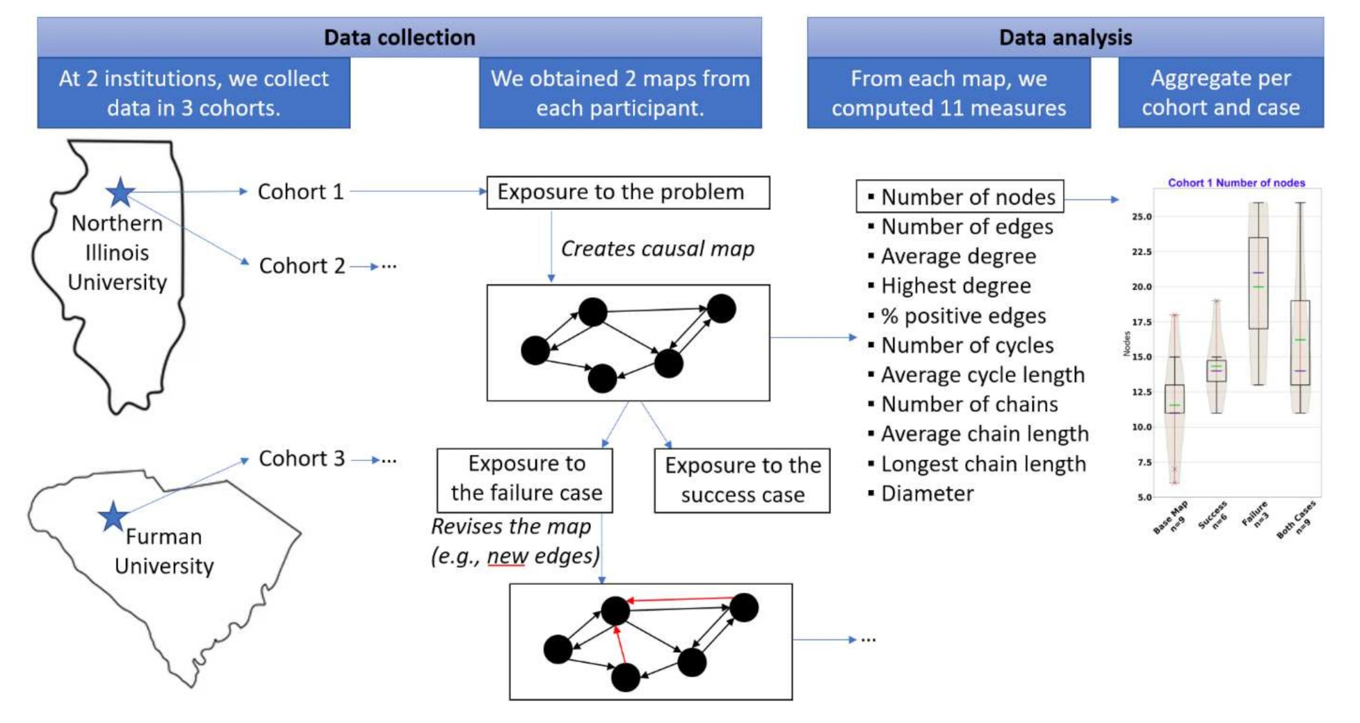
Our overall approach is summarized in Figure 2 and detailed in the next subsection. Given the complexity of the data pre-processing, we provide it as a separate schema (Figure 3).
2.1. Data Collection
Our data consists of causal maps, which are represented as graphs consisting of labelled nodes and directed, weighted edges. Each causal map was produced by a student. We collected causal maps over three semesters at two different American institutions. Northern Illinois University is a nationally-ranked public Midwestern university, in which the data collection took place through a fourth-year elective on Network Science. Furman University is a nationally-ranked private liberal arts college in the Southeast, where the data collection similarly took place during a third-year elective on Artificial Intelligence. At both institutions, the students first learned how to structure knowledge into causal maps [5], and then they were given the same baseline description of a hypothetical town (‘Pleasantville’) in which they had to advise the mayor on an open-ended dilemma (see Supplementary Material 1). In our study, the ill-structured problem required students to either accept a retailer, which would transform the city’s park into warehouses but bring jobs and tax revenues, or to decline the retailer and preserve the park but struggle with expenses such as teachers’ salaries. The students also had to consider the impact of pollution, the available natural resources, and other variables. The students then produced a causal map with the assistance of software (Python in the fourth year course or Actionable Systems in the third year course).
After the students completed their base map without scaffolding, they were introduced to success or failure cases which were relevant to the problem to solve, and were asked to revise their causal maps. The instructions for the failure case are provided in Supplementary Material 2, while the success case is given as Supplementary Material 3. For example, the successful case helped the students manage the effects of rapid population growth, while the failure cases depicted the negative effects of urbanization on the environment.
2.2. Data Cleaning/Pre-Processing
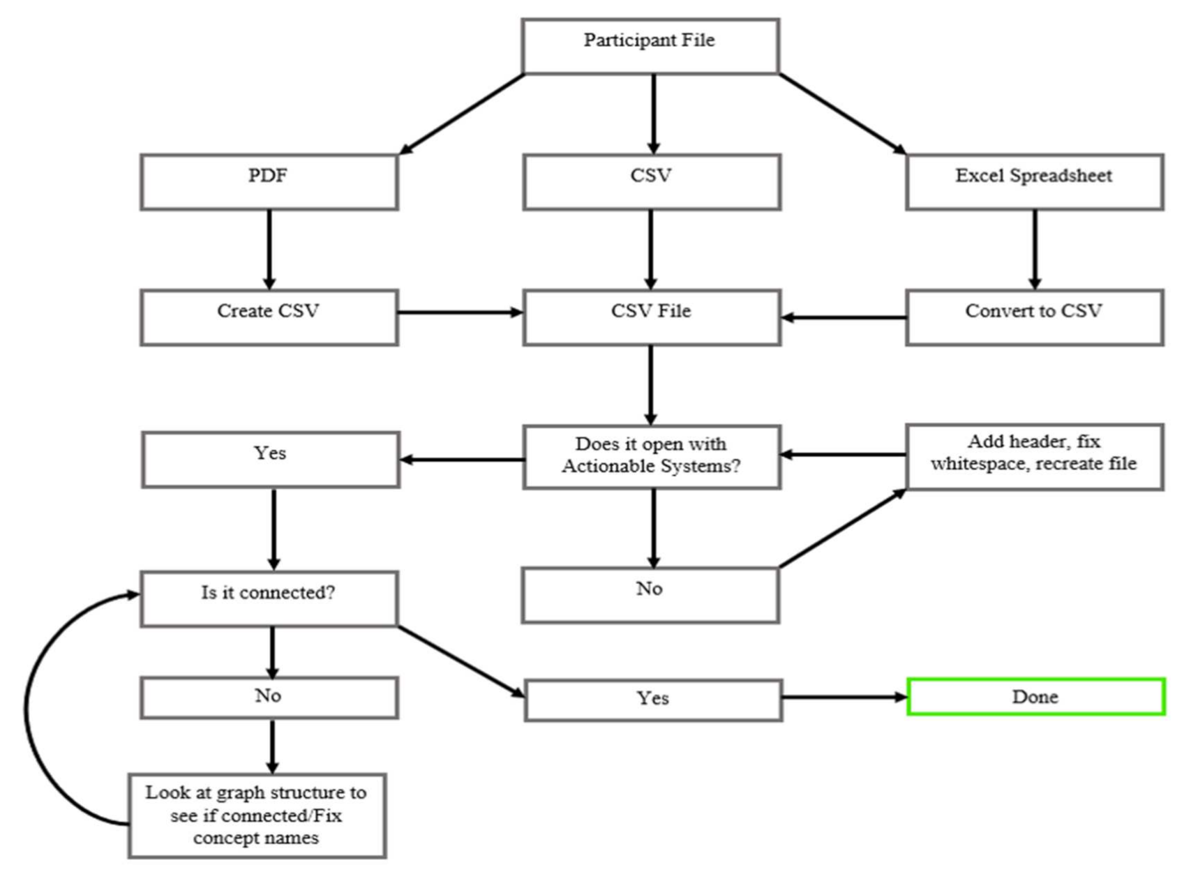
Our overall data cleaning process is shown in Figure 3. We converted the students’ submissions into one file format (CSV) for analysis. As each file encodes one causal map, we ensured that the files were consistently formatted to describe a network as a list of edges. That is, each line lists the starting node, end node, and type of the causal edge (−1 for causal decrease and 1 for causal increase). This process of ensuring that the maps were properly entered in the file was semi-automatized by using ActionableSystems [40] to detect the presence of formatting errors (e.g., missing header line, extra spaces) and then solving them manually. A common problem was the presence of typos (e.g., “Parks -> Environmental well-being”, “Parks ->Enviornmental well-being”), which would mislead the analysis into counting two distinct factors, “Environmental well-being” and “Enviornmental well-being”. Such typos were identified via ActionableSystems, as they result in a map that is visibly disconnected; they were then fixed manually.
Figure 3.
Our data cleaning process started with a participant file (top) and proceeded until we were done cleaning its content.
Figure 3.
Our data cleaning process started with a participant file (top) and proceeded until we were done cleaning its content.

As participants constructed their revised maps, rather than having them provide a discrete numeric value, they were asked to simply provide a nominal label (e.g., ‘very strong’) to describe the relations between the concepts. After the general data cleaning, we shifted to transforming the nominal values intuitively chosen by the participating students to numeric values (Table 1). These values are only used in the subsequent analysis to identify whether an edge is negative or positive.
2.3. Data Analysis
When analysing the changes between the two maps, there are several metrics which denote a more complex understanding of the problem. For example, the presence of chains typically denotes a less complex map, while the presence of cycles shows a stronger understanding of the relationships between various concepts [41]. A participant’s coverage of the problem space can be determined by the number of nodes and edges, as well as the length of their map’s diameter. Maps containing more nodes and edges have a broader scope, which may show that the participant is examining the problem in a larger context, but could also be a result of the participant going on a tangential train of thought [42,43]. The complexity of a concept map can be analysed by finding the number of cycles and chains, as well as by looking at their lengths [41].
The metrics chosen in this study to contrast the base map with the success or failure maps were selected based on their relation to the complexity of the map and the coverage of the problem space. As discussed by Frerichs et al. [44], the metrics cover the breadth, depth, and structural complexity of conceptualizations of the problem space. Note that our objective is to characterize the structure of the maps rather than to aggregate or compare the content of the maps, which would require us to either solve linguistic variability (i.e., the possibility that students use different terms to cover the same concept) or constraint students into using a bank of concepts [45] instead of letting students express concepts as they see fit (i.e., using an open-ended approach [46]). We used each metric for the following reasons:
- Number of nodes and number of edges, which represent the number of concepts and causal relationships, respectively. These simple and common measures [42] serves to evaluate whether a map covers more of the problem space.
- Average and maximum number of edges per node, also known as the ‘degree’, which measure the connectivity. Higher numbers are more important, as they indicate that students often see them as part of the problem space, exhaustively considering the causal impact of their factors.
- Diameter, which measures the furthest away that two concepts can be (i.e., the length of the longest shortest path). A very large diameter is a risk of going on a tangent (as students may go beyond the boundaries of the problem space), whereas a very small diameter may be indicative of an early map, in which most concepts are tightly packed around a focal point. A medium diameter is thus most desirable.
- Total number and average lengths of cycles. Cycles or ‘feedback loops’ are essential structures in complex problems [47]. In contrast with the simple notion of a ‘root cause’ that would need to be solved for the solution to straightforwardly permeate to a whole system, a cycle recognizes that an intervention will eventually affect us back [48], possibly in unintended ways. As cycles are often present in systems, but are harder to capture in maps due to cognitive limitations [49], seeing cycles in maps is associated with demonstrating a better understanding of the problem. We characterize cycles both in numbers (the more, the better) and in their average length (the longer, the better).
- Total number, longest length, and average length of chains. Chains or ‘paths’ indicate chains of reasoning. They reveal how students combine concepts into a logical sequence, thus giving an insight into how students associate terms and causal reasoning [27,50]. We characterized chains in their amount, and maximum and average length. Lower numbers are associated with more refined maps.
- Percentage of positive causations. Because each causal edge was categorized as either positive (i.e., an increase in A causes an increase in B) or negative (i.e., an increase in A causes a decrease in B), we measured the percentage of positive edges. The positive and negative weights are known as ‘signs’ in the framework of signed graphs, which has been the subject of recent studies in control and systems theory [51,52]. Some of the notions above (e.g., cycles) can be extended within the context of signed graphs, such as characterizing a ‘balanced network’ as having no cycle of which the product of signs is negative [53,54]. However, these refinements are more applicable to the study of polarizing phenomena [55] in social networks, in which nodes refer to individuals, and edges characterize their interactions (e.g., cooperative or antagonistic), than in the mapping of the problem spaces studied here.
These metrics were primarily computed using the NetworkX Python library within a Jupyter notebook. We note that this library offers sufficiently efficient implementations given the network sizes encountered in this paper, but readers interested in much larger networks may consider alternative approaches, such as the use of spectral graph theory to quickly characterize loops [56,57]. Graphs were generated from .csv files into NetworkXDiGraphs objects, which were then analysed using a mixture of built-in NetworkX functions and our own implementations of classic graph algorithms. The implementation of the algorithms is described in Table 2.
3. Results
The results are summarized in Table 3 and Table 4, while the sample distributions for the number of nodes and edges are shown in Figure 4 and Figure 5; all of the other distributions are provided as supplementary online material. In the first and third cohort, there is a noticeable increase in the number of edges added. This displays an increased coverage of the problem space, hinting that the participants were considering the relationships between their concepts more heavily than in their initial maps. This increase was especially pronounced in the success groups for these two cohorts. In the third cohort, this may have been a result of several outliers, who displayed a significantly larger increase in their number of edges than the others in their group. This same spike in the number of edges is likely the cause of the massive increase in cycles for the third cohort, in which the total number of cycles grew from 68 to 747 cycles after their revision. This increase stands out, as the first cohort group did not experience an increase in cycles anywhere near as significant (only 22 to 36 cycles) despite also having significant growth in the number of edges.
The number of chains and their length saw similar changes across both the success and failure group in the first two cohorts. For the first cohort, we noted a decrease in the number of chains, and their average length shortened significantly after their revisions, while the second cohort saw a small increase across both groups.
The third cohort, however, saw the introduction of chains in the success group where there were previously no chains, and the failure group saw a spike in the number of chains (4 to 38) and their length (4 to 11).
The connectivity of the graphs did not change significantly across each group, with few exceptions: the failure group in the first cohort and the success group in the third cohort, which saw a minor increase in diameter; and the failure group of the third cohort, which had a decrease in the average degree across the graph. This decrease in the average degree may be linked to the spike in chains, because an increase in chains should lower the average degree if the only new connections were those chains.
4. Discussion
4.1. Rationale for the Study and Application Context
When we do not have expertise in an application domain and still need to make decisions, our understanding of the domain can be improved by being exposed to an evidence base in the form of case studies (i.e., a ‘case library’). However, the content of the cases can have an impact on our perspectives, such that our mental model may be shaped differently depending on whether the case studies depict successful interventions or failures. Previous studies have abundantly documented that cases can support students, using a variety of metrics such as test scores. In the present study, we took one step further in examining the ways in which the perceptions of a system change as a function of exposure to certain types of evidence. Specifically, our study measured the representation of knowledge through causal maps before and after exposure to a case. We focused on causal maps as they have been used repeatedly in the literature on participatory modelling to elicit mental models with crowds that did not necessarily have prior experience in systems thinking. We acknowledge that other representations may yield different results, as mapping techniques capture specific aspects of a student’s knowledge, and hence are not interchangeable [58].
4.2. Main Takeaways from the Analysis
We found that exposure to cases leads to a higher number of nodes, edges, cycles, and a higher average degree. The diameter is not changed significantly, which provides evidence of knowledge integration. However, these numbers are increased differently depending on the case and student cohort (either Northern Illinois University fourth year students for cohorts 1–2, or Furman University third year students for cohort 3). Similarly, the findings are nuanced by case and semester for the two key structures consisting of chains and cycles. As discussed earlier, the presence of cycles is tied to a more complex understanding of the problem space [41,47,48], and chains typically denote a naïve understanding. In the first two cohorts, students used the success case to reinforce their own map, thus leading to a sharp increase in the number of cycles and their average length, while these two metrics did not noticeably change in the third cohort. The first two cohorts doubled the number of concept nodes when exposed to a failure case, as they thought of concepts which were previously unaccounted for, while the number of nodes in the third cohort increased slightly regardless of the case. Finally, the first two cohorts had noticeably more positive causal connections when they were exposed to the success case than the failure case, but this relation reversed in the third cohort.
4.3. Limitations
A potential limitation of this study was the size of the data sets. First, the activity of representing a system through several maps is time consuming for students; hence, it needs to be part of the relevant learning outcomes for the course. We thus tied it to courses on network science (focusing on the structure of knowledge as a map) or artificial intelligence (echoing the core notion of knowledge representation), which means that we performed data collection in upper-level electives which generally have small enrolment numbers at the two institutions considered, in comparison with introductory courses. We addressed this concern by collecting data for three successive semesters, thus achieving a sample size of n = 28 for the analysis. Although there is no typical number of participants for studies that elicit systems in the form of maps, we note that our sample size is comparable to several other works, with n = 27 [59] or n = 30 [60] participants. The number of participants can differ widely depending on the objectives of the study: our analysis of maps provided solely by experts had as few as n = 7 participants [61], while our examination of mental models in the community involved as many as n = 264 individuals [10]. The specific data collection protocol also plays an important role in determining whether a study can scale to many participants. Studies with very few participants can involve long one-on-one semi-structured interviews which are then transcribed and turned into maps [42], whereas studies with many participants consist of self-administered surveys in which even the choice of names for each factor is limited. The intermediate order of magnitude of our sample is in line with the intermediate option taken in this study: students can independently create maps representing their view of the system, without being forced to choose from limited options.
5. Conclusions
Effective problem solving starts with a systematic process to define the problem space and articulate the causal relationships among the variables identified. By mapping the major variables and their causal relationships, the plausible solutions will be more easily and efficiently identified [16]. In problem-based instruction, these mapping processes also help students to construct the knowledge acquired into a conceptual framework for that problem. Therefore, constructing a representation of a system by mapping the problem spaces using causal reasoning is a critical cognitive process not only to successfully solve a given problem, but also for the refinement of the students’ conceptual knowledge and problem-solving skills.
Our study shows that providing students with cases tends to broaden their coverage of the problem space, as evidenced by an increase in the number of nodes and causal edges. However, the knowledge afforded by the cases is integrated into the students’ maps differently depending on the type of case (success vs. failure) as well as the cohort of students.
Future studies could expand the data sets by continuing to recruit cohorts. Furthermore, our findings that some of the structural changes depend on the cohort suggest that additional factors may underpin the ways in which students process cases. Consequently, it would be of particular interest for future studies to also collect data about the profile of the students, and to test for the presence of mediating factors (e.g., using structural equation models) in the way that maps change when they are exposed to certain cases.
Supplementary Materials
The following are available online at https://0-www-mdpi-com.brum.beds.ac.uk/article/10.3390/systems9020023/s1: activity statement distributed to all students (S1) followed by exposure to the failure case (S2) and success case (S3); distributions across cohorts of average degree, highest degree, and percentage of positive edges (S4); distributions across cohorts of the number of cycles and average cycle length (S5); distributions across cohorts of the number of chains, average and highest chain lengths (S6); distributions across cohorts of the diameter (S7).
Author Contributions
P.J.G. and A.A.T. jointly designed the study. P.J.G. collected the data and directed the analysis. P.J.G. and A.A.T. jointly wrote and approved the manuscript. All authors have read and agreed to the published version of the manuscript.
Funding
P.J.G. thanks Furman University for helping support this research through the Furman Advantage.
Informed Consent Statement
Informed consent was obtained from all subjects involved in the study.
Data Availability Statement
Our detailed study protocols and distributions are provided as supplementary materials. Anonymized assignments can be shared upon request to the corresponding author.
Acknowledgments
We are indebted to Max L. Norman for assisting with the analysis of the data and providing input on earlier versions of this manuscript.
Conflicts of Interest
The authors declare no conflict of interest.
References
- Voinov, A.; Jenni, K.; Gray, S.; Kolagani, N.; Glynn, P.D.; Bommel, P.; Prell, C.; Zellner, M.; Paolisso, M.; Jordan, R.; et al. Tools and methods in participatory modeling: Selecting the right tool for the job. Environ. Model. Softw. 2018, 109, 232–255. [Google Scholar] [CrossRef] [Green Version]
- Walsh, R. Narrative theory for complexity scientists. In Narrating Complexity; Springer: Cham, Switzerland, 2018; pp. 11–25. [Google Scholar]
- Goldstein, B.E.; Wessells, A.T.; Lejano, R.; Butler, W. Narrating resilience: Transforming urban systems through collaborative storytelling. Urban. Stud. 2015, 52, 1285–1303. [Google Scholar] [CrossRef]
- Berg, T.; Pooley, R. Contemporary iconography for rich picture construction. Syst. Res. Behav. Sci. 2013, 30, 31–42. [Google Scholar] [CrossRef]
- De Pinho, H. Mapping Complex Systems of Population Health. In Systems Science and Population Health; El-Sayed, A.M., Galea, S., Eds.; Oxford University Press: Oxford, UK, 2017; pp. 61–76. [Google Scholar]
- Bala, B.K.; Arshad, F.M.; Noh, K.M. Causal loop diagrams. In System Dynamics; Springer: Singapore, 2017; pp. 37–51. [Google Scholar]
- Moon, B.; Hoffman, R.R.; Novak, J.; Canas, A. (Eds.) Applied Concept Mapping: Capturing, Analyzing, and Organizing Knowledge; CRC Press: Boca Raton, FL, USA, 2011. [Google Scholar]
- Gray, S.; Sterling, E.J.; Aminpour, P.; Goralnik, L.; Singer, A.; Wei, C.; Akabas, S.; Jordan, R.C.; Giabbanelli, P.J.; Hodbod, J.; et al. Assessing (social-ecological) systems thinking by evaluating cognitive maps. Sustainability 2019, 11, 5753. [Google Scholar] [CrossRef] [Green Version]
- Reddy, T; Giabbanelli, P.J; Mago, V.K. The artificial facilitator: Guiding participants in developing causal maps using voice-activated technologies. In Proceedings of the International Conference on Human-Computer Interaction, Copenhagen, Denmark, 26 July 2019; Springer: Cham, Switzerland, 26 July 2019; pp. 111–129. [Google Scholar]
- Lavin, E.A.; Giabbanelli, P.J.; Stefanik, A.T.; Gray, S.A.; Arlinghaus, R. Should we simulate mental models to assess whether they agree? In Proceedings of the Annual Simulation Symposium, Baltimore, MD, USA, 15 April 2018; pp. 1–12. [Google Scholar]
- Gray, S.; Hilsberg, J.; McFall, A.; Arlinghaus, R. The structure and function of angler mental models about fish population ecology: The influence of specialization and target species. J. Outdoor Recreat. Tour. 2015, 12, 1–3. [Google Scholar] [CrossRef]
- Douglas, E.M.; Wheeler, S.A.; Smith, D.J.; Overton, I.C.; Gray, S.A.; Doody, T.M.; Crossman, N.D. Using mental-modelling to explore how irrigators in the Murray–Darling Basin make water-use decisions. J. Hydrol. Reg. Stud. 2016, 6, 1–2. [Google Scholar] [CrossRef] [Green Version]
- Drasic, L.; Giabbanelli, P.J. Exploring the interactions between physical well-being, and obesity. Can. J. Diabetes 2015, 39, S12–S13. [Google Scholar] [CrossRef]
- Finegood, D.T; Merth, T.D; Rutter, H. Implications of the foresight obesity system map for solutions to childhood obesity. Obesity 2010, 18, S13. [Google Scholar] [CrossRef]
- Rahimi, N.; Jetter, A.J.; Weber, C.M.; Wild, K. Soft Data analytics with fuzzy cognitive maps: Modeling health technology adoption by elderly women. In Advanced Data Analytics in Health; Springer: Cham, Switzerland, 2018; pp. 59–74. [Google Scholar]
- Eseryel, D.; Ifenthaler, D.; Ge, X. Validation study of a method for assessing complex ill-structured problem solving by using causal representations. Educ. Technol. Res. Dev. 2013, 61, 443–463. [Google Scholar] [CrossRef]
- Ifenthaler, D.; Masduki, I.; Seel, N.M. The mystery of cognitive structure and how we can detect it: Tracking the development of cognitive structures over time. Instr. Sci. 2011, 39, 41–61. [Google Scholar] [CrossRef]
- Trumpower, D.L.; Filiz, M.; Sarwar, G.S. Assessment for learning using digital knowledge maps. In Digital Knowledge Maps in Education; Springer: New York, NY, USA, 2014; pp. 221–237. [Google Scholar]
- Giabbanelli, P.J.; Tawfik, A.A. Reducing the Gap Between the Conceptual Models of Students and Experts Using Graph-Based Adaptive Instructional Systems. In Proceedings of the International Conference on Human-Computer Interaction, Copenhagen, Denmark, 19–24 July 2020; Springer: Cham, Switzerland, 2020; pp. 538–556. [Google Scholar]
- Giabbanelli, P.J.; Tawfik, A.A. Overcoming the PBL assessment challenge: Design and development of the incremental thesaurus for assessing causal maps (ITACM). Technol. Knowl. Learn. 2019, 24, 161–168. [Google Scholar] [CrossRef]
- Giabbanelli, P.J.; Tawfik, A.A.; Gupta, V.K. Learning analytics to support teachers’ assessment of problem solving: A novel application for machine learning and graph algorithms. Util. Learn. Anal. Support Study Success 2019, 175–199. [Google Scholar] [CrossRef]
- Hmelo-Silver, C.E. Creating a learning space in problem-based learning. Interdiscip. J. Probl. Based Learn. 2013, 7, 5. [Google Scholar] [CrossRef] [Green Version]
- Jonassen, D.H. Learning to Solve Problems: A Handbook for Designing Problem-Solving Learning Environments. Routledge: New York, NY, USA, 2010. [Google Scholar]
- Malhi, L.; Karanfil, Ö.; Merth, T.; Acheson, M.; Palmer, A.; Finegood, D.T. Places to intervene to make complex food systems more healthy, green, fair, and affordable. J. Hunger Environ. Nutr. 2009, 4, 466–476. [Google Scholar] [CrossRef] [Green Version]
- Dufresne, R.J.; Gerace, W.J.; Hardiman, P.T.; Mestre, J.P. Constraining novices to perform expert-like problem analyses: Effects on schema acquisition. J. Learn. Sci. 1992, 2, 307–331. [Google Scholar] [CrossRef]
- Jeong, A. Sequentially analyzing and modeling causal mapping processes that support causal understanding and systems thinking. In Digital Knowledge Maps in Education; Springer: New York, NY, USA, 2014; pp. 239–251. [Google Scholar]
- Shin, H.S.; Jeong, A. Modeling the relationship between students’ prior knowledge, causal reasoning processes, and quality of causal maps. Comput. Educ. 2021, 163, 104113. [Google Scholar] [CrossRef]
- Hmelo-Silver, C.E.; Marathe, S.; Liu, L. Fish swim, rocks sit, and lungs breathe: Expert-novice understanding of complex systems. J. Learn. Sci. 2007, 16, 307–331. [Google Scholar] [CrossRef]
- Stefaniak, J. The utility of design thinking to promote systemic instructional design practices in the workplace. TechTrends 2020, 64, 202–210. [Google Scholar] [CrossRef]
- Zhou, C.; Chai, C.; Liao, J. Analysis of problem decomposition strategies of novice industrial designers using network-based cognitive maps. Int. J. Technol. Des. Educ. 2021, 25, 1–23. [Google Scholar]
- Metcalf, S.J.; Reilly, J.M.; Kamarainen, A.M.; King, J.; Grotzer, T.A.; Dede, C. Supports for deeper learning of inquiry-based ecosystem science in virtual environments-Comparing virtual and physical concept mapping. Comput. Hum. Behav. 2018, 87, 459–469. [Google Scholar] [CrossRef]
- Martin, W.; Silander, M.; Rutter, S. Digital games as sources for science analogies: Learning about energy through play. Comput. Educ. 2019, 130, 1–2. [Google Scholar] [CrossRef]
- Whitelock-Wainwright, A.; Laan, N.; Wen, D.; Gašević, D. Exploring student information problem solving behaviour using fine-grained concept map and search tool data. Comput. Educ. 2020, 145, 103731. [Google Scholar] [CrossRef]
- Burkhart, C.; Lachner, A.; Nückles, M. Assisting students’ writing with computer-based concept map feedback: A validation study of the CohViz feedback system. PLoS ONE 2020, 15, e0235209. [Google Scholar] [CrossRef]
- Lachner, A.; Burkhart, C.; Nückles, M. Formative computer-based feedback in the university classroom: Specific concept maps scaffold students’ writing. Comput. Hum. Behav. 2017, 72, 459–469. [Google Scholar] [CrossRef]
- Tawfik, A.A.; Gill, A.; Hogan, M.; York, C.S.; Keene, C.W. How novices use expert case libraries for problem solving. Technol. Knowl. Learn. 2019, 24, 23–40. [Google Scholar] [CrossRef]
- Hernandez-Serrano, J.; Jonassen, D.H. The effects of case libraries on problem solving. J. Comput. Assist. Learn. 2003, 19, 103–114. [Google Scholar] [CrossRef]
- Tawfik, A.A.; Alhoori, H.; Keene, C.W.; Bailey, C.; Hogan, M. Using a Recommendation System to Support Problem Solving and Case-Based Reasoning Retrieval. Technol. Knowl. Learn. 2018, 23, 177–187. [Google Scholar] [CrossRef]
- Schank, R.C. Dynamic Memory Revisited. Cambridge University Press: Cambridge, UK, 1999. [Google Scholar]
- Giabbanelli, P.J.; Baniukiewicz, M. Navigating complex systems for policymaking using simple software tools. In Advanced Data Analytics in Health; Springer: Cham, Switzerland, 2018; pp. 21–40. [Google Scholar]
- Shute, V.J.; Zapata-Rivera, D. Using an evidence-based approach to assess mental models. In Understanding Models for Learning and Instruction; Springer: Boston, MA, USA, 2008; pp. 23–41. [Google Scholar]
- Firmansyah, H.S.; Supangkat, S.H.; Arman, A.A.; Giabbanelli, P.J. Identifying the components and interrelationships of smart cities in Indonesia: Supporting policymaking via fuzzy cognitive systems. IEEE Access 2019, 7, 46136–46151. [Google Scholar] [CrossRef]
- Brandes, U. Network Analysis: Methodological Foundations. Springer Science & Business Media: Berlin/Heidelberg, Germany, 2005. [Google Scholar]
- Frerichs, L.; Young, T.L.; Dave, G.; Stith, D.; Corbie-Smith, G.; Lich, K.H. Mind maps and network analysis to evaluate conceptualization of complex issues: A case example evaluating systems science workshops for childhood obesity prevention. Eval. Program Plan. 2018, 68, 135–147. [Google Scholar] [CrossRef]
- Bergan-Roller, H.E.; Galt, N.J.; Helikar, T.; Dauer, J.T. Using concept maps to characterise cellular respiration knowledge in undergraduate students. J. Biol. Educ. 2020, 54, 33–46. [Google Scholar] [CrossRef]
- De Ries, K.E.; Schaap, H.; van Loon, A.M.; Kral, M.M.; Meijer, P.C. A literature review of open-ended concept maps as a research instrument to study knowledge and learning. Qual. Quant. 2021, 1–35. [Google Scholar] [CrossRef]
- Giabbanelli, P.J. Analyzing the complexity of behavioural factors influencing weight in adults. In Advanced Data Analytics in Health; Springer: Cham, Switzerland, 2018; pp. 163–181. [Google Scholar]
- Fink, D.S.; Keyes, K.M. When simple interpretations create complex problems. Syst. Sci. Popul. Health 2017, 1, 3. [Google Scholar]
- Axelrod, R. (Ed.) Structure of Decision: The Cognitive Maps of Political Elites. Princeton University Press: Princeton, NJ, USA, 2015. [Google Scholar]
- Tawfik, A.A.; Hung, W.; Giabbanelli, P.J. Comparing How Different Inquiry-Based Approaches Impact Learning Outcomes. Interdiscip. J. Probl. -Based Learn. 2020, 14, n1. [Google Scholar] [CrossRef]
- Tselykh, A.; Vasilev, V.; Tselykh, L.; Ferreira, F.A. Influence control method on directed weighted signed graphs with deterministic causality. Ann. Oper. Res. 2020, 1–25. [Google Scholar] [CrossRef]
- Tselykh, A.; Vasilev, V.; Tselykh, L. Assessment of influence productivity in cognitive models. Artif. Intell. Rev. 2020, 1–27. [Google Scholar] [CrossRef]
- Cartwright, D.; Harary, F. Structural balance: A generalization of Heider’s theory. Psychol. Rev. 1956, 63, 277. [Google Scholar] [CrossRef] [Green Version]
- Davis, J.A. Clustering and structural balance in graphs. Hum. Relat. 1967, 20, 181–187. [Google Scholar] [CrossRef]
- Patel, I.; Nguyen, H.; Belyi, E.; Getahun, Y.; Abdulkareem, S.; Giabbanelli, P.J.; Mago, V. Modeling information spread in polarized communities: Transitioning from legacy media to a Facebook world. In SoutheastCon 2017; IEEE: New York, NY, USA, 2017; pp. 1–8. [Google Scholar]
- Chung, F.R.; Graham, F.C. Spectral Graph Theory. American Mathematical Society: Providence, RI, USA, 1997. [Google Scholar]
- Godsil, C.; Royle, G.F. Algebraic Graph Theory. Springer Science & Business Media: Cham, Switzerland, 2001. [Google Scholar]
- Yin, Y.; Vanides, J.; Ruiz-Primo, M.A.; Ayala, C.C.; Shavelson, R.J. Comparison of two concept-mapping techniques: Implications for scoring, interpretation, and use. J. Res. Sci. Teach. 2005, 42, 166–184. [Google Scholar] [CrossRef] [Green Version]
- Gray, S.; Chan, A.; Clark, D.; Jordan, R. Modeling the integration of stakeholder knowledge in social–ecological decision-making: Benefits and limitations to knowledge diversity. Ecol. Model. 2012, 229, 88–96. [Google Scholar] [CrossRef]
- Papageorgiou, E.; Kontogianni, A. Using fuzzy cognitive mapping in environmental decision making and management: A methodological primer and an application. In International Perspectives on Global Environmental Change; IntechOpen: London, UK, 2011; pp. 427–450. [Google Scholar]
- Giabbanelli, P.J.; Torsney-Weir, T.; Mago, V.K. A fuzzy cognitive map of the psychosocial determinants of obesity. In Appl. Soft Comput.; 2012; Volume 12, pp. 3711–3724. [Google Scholar]
Figure 1.
Three different mapping approaches: Novakian concept maps are usually acyclic graphs, specifying relationships using labels to form sentences (a); Causal Loop Diagrams are a precursor to the System Dynamics model, and include temporal aspects such as delays (b); Causal maps only include the type of causation, and thus temporality is not represented (c).

Figure 2.
Workflow of our study, from data collection to analysis. Each step is detailed in this section.
Figure 2.
Workflow of our study, from data collection to analysis. Each step is detailed in this section.

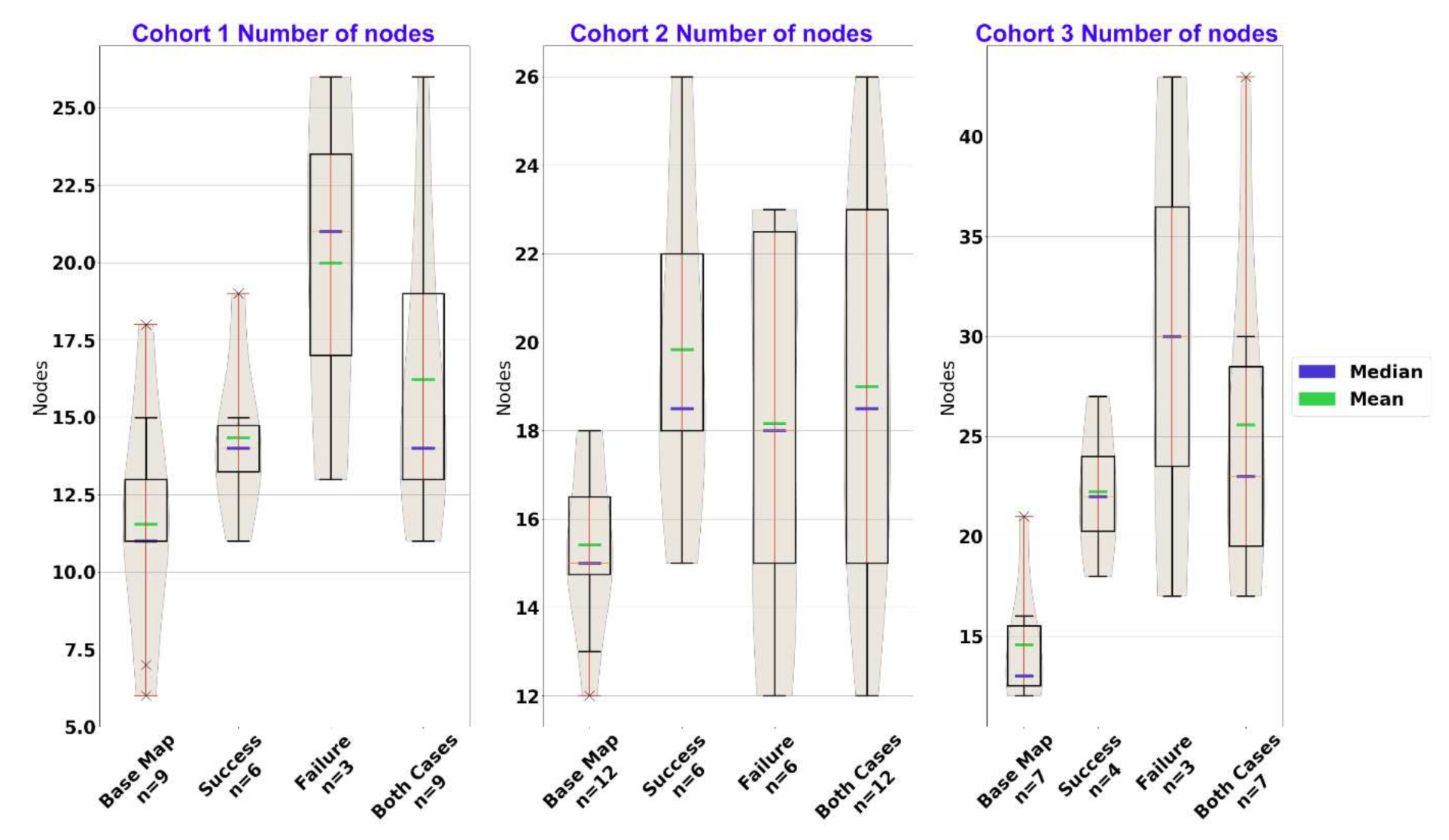
Figure 4.
Exposure to cases resulted in a higher number of nodes across all of the cohorts, as seen in the difference between the leftmost (baseline) and rightmost (after cases) distributions. However, the different effects of the success and failure cases depend on the cohort: cohort 2 gained about as many nodes in either the success or failure cases, while the other cohorts gained most from the failure case.

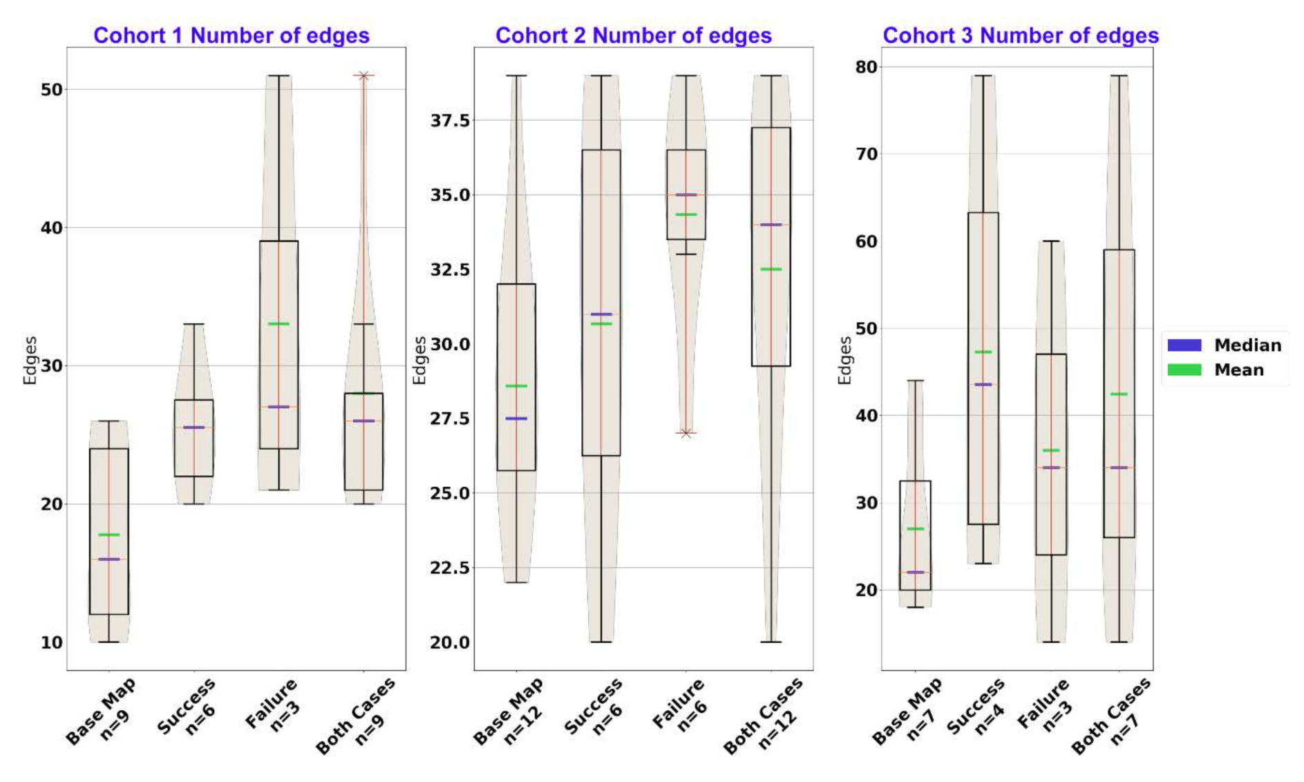
Figure 5.
Exposure to cases resulted in a higher number of edges across all cohorts, as seen in the difference between the leftmost (baseline) and rightmost (after cases) distributions. Cohorts 1 and 2 gained most from the failure case, but cohort 3 gained most from the success case.
Figure 5.
Exposure to cases resulted in a higher number of edges across all cohorts, as seen in the difference between the leftmost (baseline) and rightmost (after cases) distributions. Cohorts 1 and 2 gained most from the failure case, but cohort 3 gained most from the success case.


Table 1.
Conversions between nominal and numeric data.
| Positive Relation | Negative Relation |
|---|---|
| Very Strong (‘VS’) = 1 | Very Strong (‘VS’) = −1 |
| Strong (‘S’) = 0.8 | Strong (‘S’) = −0.8 |
| Medium (‘M’) = 0.6 | Medium (‘M’) = −0.6 |
| Low (‘L’) = 0.4 | Low (‘L’) = −0.4 |
| Very Low (‘VL’) = 0.2 | Very Low (‘VL’) = −0.2 |
Table 2.
Description of each metric and what they measure, along with how they are implemented.
| Measure | Metric | Implementation |
|---|---|---|
| Complexity | Average length and number of cycles | Found by using NetworkX’s simple_cycles function and sorting the nodes in the cycle before passing it into a set to remove duplicates. |
| Average length, longest, and number of chains | Found by getting all shortest paths between nodes using NetworkX’s shortest_simple_paths function and counting those whose paths contain only nodes of degree two or higher. | |
| Coverage of Problem Space | Number of nodes and edges | Counted the number of nodes and edges in the graph. |
| Diameter | Found the longest of the shortest paths found using NetworkX’s shortest_simple_paths function. | |
| Type of causations | Percentage of positive causations | Found by reading the last column in the .csv files and checking if the value is above zero, if so find add to count and divide the final count by the total number of rows in the file. |
Table 3.
Relative differences of the students’ maps for each group (success, failure), and for all students combined. The first two cohorts were formed at Northern Illinois University in a fourth-year elective on network science, while the third cohort originated from Furman University through a third-year course on artificial intelligence.
| Difference | ||||||||||
|---|---|---|---|---|---|---|---|---|---|---|
| Cohort 1 | Cohort 2 | Cohort 3 | ||||||||
| Both Cases (n = 9) | Success(n = 6) | Failure(n = 3) | Both Cases(n = 12) | Success(n = 6) | Failure(n = 6) | BothCases(n = 7) | Success(n = 4) | Failure(n = 3) | ||
| Cycles | Total | + | + | = | + | = | + | ++ | ++ | - |
| AverageLength | + | + | = | = | - | = | = | + | = | |
| Elements | Number of Nodes | + | = | ++ | = | = | = | ++ | ++ | ++ |
| Number of Edges | ++ | + | ++ | = | = | = | ++ | ++ | + | |
| Connectivity | Diameter | = | = | + | = | = | = | = | + | = |
| Average Degree | = | = | = | = | = | = | = | = | - | |
| Chains | Total | -- | -- | -- | ++ | + | ++ | ++ | N/A * | ++ |
| Longest | -- | -- | -- | ++ | ++ | ++ | ++ | ++ | ||
| Average Length | -- | -- | -- | ++ | ++ | + | ++ | ++ | ||
+ is a greater than 25% increase from the previous map, ++ is a greater than 50% increase from the previous map. - is a greater than 25% decrease from the previous map, -- is a greater than 50% decrease from the previous map. = is a change of less than a 25% (either increase or decrease) from the previous map. * None of the four students had chains to start with. In the success group, two of them added chains: one added one chain (of length 2), and the other added five chains (of length 2 to 3, with 2.2 on average).
Table 4.
Absolute measurements in each map for each group of students (success and failure are reported separately).
Table 4.
Absolute measurements in each map for each group of students (success and failure are reported separately).
| Difference | |||||||||||||
|---|---|---|---|---|---|---|---|---|---|---|---|---|---|
| Cohort 1 | Cohort 2 | Cohort 3 | |||||||||||
| Baseline Success Group(n = 6) | After Exposure to Success Case(n = 6) | Baseline Failure Group(n = 3) | After Exposure to Failure Case(n = 3) | Baseline Success Group(n = 6) | After Exposure to Success Case(n = 6) | Baseline Failure(n = 6) | After Exposure to Failure Case(n = 6) | BaselineSuccess Group(n = 4) | After Exposure to Success Case(n = 4) | BaselineFailure Group(n = 3) | After Exposure to Failure Case(n = 3) | ||
| Cycles | Total | 22.00 | 36.00 | 0.00 | 0.00 | 92.00 | 114.00 | 75.00 | 103.00 | 68.00 | 747.00 | 48.00 | 27.00 |
| AverageLength | 10.65 | 10.65 | 0.00 | 0.00 | 21.07 | 16.01 | 21.63 | 22.13 | 16.79 | 21.29 | 12.65 | 11.16 | |
| Elements | Number of Nodes | 71.00 | 86.00 | 33.00 | 60.00 | 96.00 | 119.00 | 89.00 | 109.00 | 53.00 | 89.00 | 49.00 | 90.00 |
| Number of Edges | 112.00 | 153.00 | 48.00 | 99.00 | 166.00 | 184.00 | 177.00 | 206.00 | 109.00 | 189.00 | 80.00 | 108.00 | |
| Connect-ivity | Diameter | 26.00 | 28.00 | 11.00 | 15.00 | 35.00 | 35.00 | 32.00 | 37.00 | 19.00 | 24.00 | 16.00 | 15.00 |
| Average Degree | 19.05 | 21.41 | 8.70 | 9.73 | 21.20 | 19.37 | 24.16 | 23.51 | 16.0 | 16.21 | 9.57 | 6.70 | |
| Chains | Total | 9.00 | 1.00 | 4.00 | 1.00 | 7.00 | 10.0 | 4.00 | 10.00 | 0.00 | 6.00 | 4.00 | 38.00 |
| Longest | 7.00 | 2.00 | 5.00 | 2.00 | 4.00 | 8.00 | 5.00 | 8.00 | 0.00 | 5.00 | 4.00 | 11.00 | |
| Average Length | 6.20 | 2.00 | 4.34 | 2.00 | 4.00 | 8.00 | 4.34 | 6.5.0 | 0.00 | 4.2.0 | 4.0 | 6.88 | |
Publisher’s Note: MDPI stays neutral with regard to jurisdictional claims in published maps and institutional affiliations. |
© 2021 by the authors. Licensee MDPI, Basel, Switzerland. This article is an open access article distributed under the terms and conditions of the Creative Commons Attribution (CC BY) license (https://creativecommons.org/licenses/by/4.0/).
Share and Cite
MDPI and ACS Style
Giabbanelli, P.J.; Tawfik, A.A. How Perspectives of a System Change Based on Exposure to Positive or Negative Evidence. Systems 2021, 9, 23. https://0-doi-org.brum.beds.ac.uk/10.3390/systems9020023
AMA Style
Giabbanelli PJ, Tawfik AA. How Perspectives of a System Change Based on Exposure to Positive or Negative Evidence. Systems. 2021; 9(2):23. https://0-doi-org.brum.beds.ac.uk/10.3390/systems9020023
Chicago/Turabian StyleGiabbanelli, Philippe J., and Andrew A. Tawfik. 2021. "How Perspectives of a System Change Based on Exposure to Positive or Negative Evidence" Systems 9, no. 2: 23. https://0-doi-org.brum.beds.ac.uk/10.3390/systems9020023
Note that from the first issue of 2016, this journal uses article numbers instead of page numbers. See further details here.