Oxygen Deficient (OD) Combustion and Metabolism: Allometric Laws of Organs and Kleiber’s Law from OD Metabolism?

Annamalai, Kalyan

doi:10.3390/systems9030054

Open AccessArticle

Oxygen Deficient (OD) Combustion and Metabolism: Allometric Laws of Organs and Kleiber’s Law from OD Metabolism?

by

Kalyan Annamalai

Department of Mechanical Engineering, Texas A&M University, College Station, TX 77843-3123, USA

Systems 2021, 9(3), 54; https://0-doi-org.brum.beds.ac.uk/10.3390/systems9030054

Submission received: 4 June 2021 / Revised: 25 June 2021 / Accepted: 2 July 2021 / Published: 16 July 2021

(This article belongs to the Section Systems Engineering)

Download

Browse Figures

Review Reports Versions Notes

Abstract

:

The biology literature presents allometric relations for the specific metabolic rate (SMR_k) of an organ k of mass mk within the body of mass m_B: SMR_k ∝ m_B^fk (body mass allometry, BMA). Wang et al. used BMA, summed-up energy from all organs and validated Kleiber’s law of the whole body: SMR_M ∝ m_B^b’, b’ = −0.25. The issues raised in biology are: (i) why f_k and b’ < 0, (ii) how do the organs adjust f_k to yield b’? The current paper presents a “system” approach involving the field of oxygen deficient combustion (ODC) of a cloud of carbon particles and oxygen deficient metabolism (ODM), and provides partial answers by treating each vital organ as a cell cloud. The methodology yields the following: (i) a dimensionless “group” number G_OD to indicate extent of ODM, (ii) SMR_k of an organ in terms of the effectiveness factor; (iii) curve fitting of the effectiveness factor to yield the allometric exponents for the organ mass-based allometric laws (OMA); (iv) validation of the results with data from 111 biological species (BS) with m_B ranging from 0.0075 to 6500 kg. The “hypoxic” condition at organ level, particularly for COVID-19 patients, and the onset of cancer and virus multiplication are interpreted in terms of ODM and glycolysis.

Keywords:

oxygen deficiency (OD); metabolism; effectiveness factor; vital organs; allometric laws; COVID-19; cancer

1. Introduction and Background

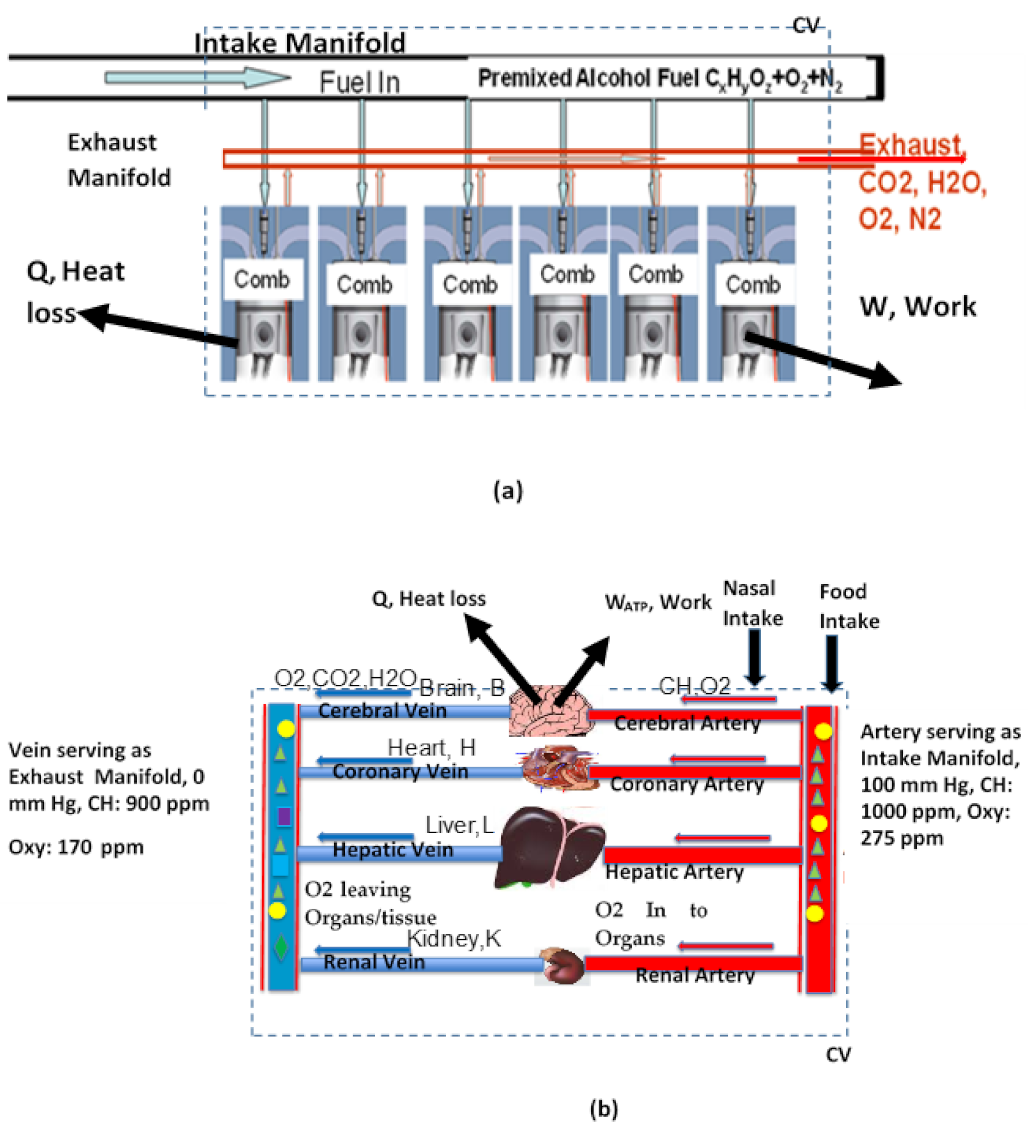
Air breathing thermal power systems, such as automobile engines, convert chemical energy into thermal energy via combustion of fuels (a high temperature oxidation) of fuels with O₂ supplied from the air. Figure 1a illustrates a multi-cylinder internal combustion engine supplied with premixed fuel and air. A part of the thermal energy in the engine is converted to useful mechanical work

\{\dot{W}\}

. The remaining energy is disposed of as heat loss

\{\dot{Q}\}

. The ratio of work output to energy input is termed as the thermal efficiency, which is about 35%. Air-breathing biological species (BS), including humans, are in many ways like those thermal systems and calorimetry and thermodynamics are strongly coupled to metabolic processes within BS [1]. Just as crude oil is refined into gasoline, diesel, and kerosene for use in thermal systems, the intestines of the digestion system of BS serve as a “food refinery” and convert food into three basic nutrients: Carbohydrates (CH, e.g., glucose), Fats (F, e.g., palmitic acid) and Proteins (P). The energy release rate (ERR, or

\dot{q}

, called metabolic rate, MR, in biology) occurs mainly through the oxidation of CH and F. Unlike rapid oxidation (combustion) of fuel in thermal systems, the BS uses a slow oxidation process to convert 2/3 of chemical energy {

\dot{q}

} into heat

\{\dot{Q}\}

, and the remaining part is converted into “chemical work”

\{{\dot{W}}_{A T P}\}

in the form of the production of adenosine triphosphate (ATP) within the organs of BS (Figure 1b). In the BS, the heat is used to overcome heat loss from BS to the surroundings and to maintain body temperature independent of the external environment (homeostasis). The body temperature of BS is about 36 °C for elephants, 37 °C for humans, and 42 °C for chickens [2]. The ATP is known as the life-sustaining work currency of the body. It is used to (i) transport nutrients, (ii) maintain the thermodynamic potential for driving reactions and species transfer, (iii) supply energy for endergonic reactions required the functioning of various organs (e.g., work for pumping blood out of heart) and (iv) provide power to propel the BS. Concentration of ATP is used to detect the presence of virions [3]. The ratio

{\dot{W}}_{A T P}

to

\dot{q}

is called the metabolic efficiency (η_M), which is typically 35%, and is somewhat similar to the thermal efficiency of an automobile. Dobson’s review on the scaling relation for BS and the estimate of lifetime ATP production seems to indicate an average metabolic efficiency of 32% [4].

The nutrients CH, F, and P obtained from digestion of food intake pass through the liver to regulate the level of CH at about 1000 ppm (5.88 mM, assuming ρ_bl = 1.060 kg/L) in the blood stream of inferior vena cava and the excess CH is stored as glycogen. Unlike CH, the O₂ cannot be stored except as oxyhemoglobin (OHb) in 5 L of human blood and hence there is a constant need for oxygen through respiration. The O₂-poor blood stream from inferior and superior vena cava enters the heart and is pumped to the lungs for enrichment with O₂, which is obtained through air breathed into the air sacs (alveoli, a vascularized sac) of the lungs. The volume of air drawn in per breath, the tidal volume, like the air drawn in during one stroke of an automobile engine, is typically 500 mL for 70 kg per person or about seven mL per kg of body mass. The O₂ exists at partial pressure of p_A,O2 in the alveoli. The O₂ is transferred from the alveoli to blood capillaries, and is subsequently dissolved into the blood where it exists at partial pressure of p_a,O2. From thermodynamics [5], the relation for concentration of dissolved O₂ (O₂, (aq)) is given by Henry’s law:

[O_{2} (a q)] \{\frac{m L o f O_{2}}{L o f B l o o d}\} = H_{O 2} \{\frac{m L o f O_{2}}{L o f B l o o d m m H g}\} p_{O 2} (m m H g), p_{O 2} = p_{A, O 2} \approx p_{a, O 2}

(1)

where H_O2 is Henry’s constant. The H_O2 is 0.021 to 0.037 mL of O₂ per L of blood per mm of Hg [6,7]. See Ref [8] for the approximation p_A,O2 ≈ p_a,O2. The p_A,O2 is about 105 mm Hg while p_a,O2 ranged from 95–100 mm Hg. While the biology literature presents oxygen content as mL of gas (CST) per L of blood, combustion literature presents this as mass fraction (Y_O2). Hence Equation (1) for dissolved oxygen is converted into the oxygen mass fraction basis:

Y_{O 2} \{\frac{g o f O_{2}}{g b l o o d}\} = H_{O 2} \{\frac{ρ_{O 2}}{ρ_{b l}}\} * 10^{(- 3)} p_{O 2} (m m H g) = 4.15 \times 10^{(- 8)} \{\frac{g o f O_{2}}{g b l o o d m m H g}\} p_{O 2} (m m H g)

(2)

Selecting H_O2 = 0.031 mL of O₂ per L per mm Hg.

Once in blood stream, the dissolved O₂ binds with the hemoglobin (Hb) in the red blood cells (RBC, 350 million Hb molecules per RBC) to produce oxy-hemoglobin (OHb) or Hb(O₂) _n, n = 1, 2, 3, 4. Thus, about 1.4 billion oxygen molecules are packed per RBC if n = 4. Eventually, chemical equilibrium is reached for Hb oxidation reactions within venous blood leaving the lungs. The equilibrium reactions are given by:

H b + n O_{2} = H b {(O_{2})}_{n}, n = 1, 2, 3, 4

(3)

K'_{n}^{0} \{\frac{1}{{(m m H g)}^{n}}\} = \{\frac{[H b {(O_{2})}_{n}]}{[H b] p_{O 2}^{n}}\}, p_{O 2} in m m H g, n = 1, 2, 3, 4

(4)

The equilibrium constants K⁰_n are given as [9]

{K'}_{1}^{0} = 0 . 01 {mm Hg}^{- 1} {, K'}_{2}^{0} = 0 . 02 {mm Hg}^{- 2} {, K'}_{3}^{0} = 0 . 04 {mm Hg}^{- 3} {, K'}_{4}^{0} = 0 . 08 {mm Hg}^{- 4}

The square parentheses in Equation (4) represent molal concentrations. The ratio of oxygen captured as OHb to the maximum that could be captured if all Hb in the blood is oxidized to Hb(O₂)₄ is the saturation fraction. The equilibrium calculations yield the plot of saturation percentage and concentration of OHb (n = 1, 2, 3, and 4) vs. p_O2 (Figure 2). The blood, which now contains the premixed CH: O₂ mixture, is pumped by the heart through large vessels (called macro vasculature) to various organs within the body.

With ρ_bl = 1060 g/L, H_O2 = 0.031 mL of O₂ per L of blood and per mm of Hg, ρ_O2 = 1.42 g/L, and 1 g of Hb holds 1.36 mL of O₂ in Hb(O₂)₄, the total oxygen {dissolved and oxygen bound oxyhemoglobin) content in blood can be shown to be:

Total oxy {, Y}_{O 2}, ppm = 0 . 182 (Hb) (\frac{g}{DL}) {Sa}_{O 2} % + 0 . 0415 p_{a, O 2} (mm Hg) .

(5)

where Sa_O2 is saturation % and (Hb) is mass concentration. See Ref. [10] also for oxygen content in terms of mL of O₂ per L of blood. Equation (5) indicates that the oxygen content in blood is controlled by three parameters: (Hb), Saturation % and arterial p_a,O2. Under normal conditions with arterial blood saturation, SaO₂ = 95 %, p_aO2 = 100 mm of Hg, (Hb) = 15 g/dL {typically, male: 14–17 g/dL, female:12–15), dissolved oxygen is computed as 4 ppm, oxygen bound to Hb is 260 ppm {oxyhemoglobin, OHb or Hb(O₂)_n, n = 1, …, 4}; i.e., total oxygen content of 264 ppm is dominated by oxy-Hb and hence almost proportional to Hb content of blood at given p_O2 and SaO₂%. The OHb serves as the carrier of oxygen. Figure 2 uses equilibrium constants and hence the total oxygen content at equilibrium is slightly different from Ref. [10] and is about 275 ppm {4.5 ppm as dissolved O₂, 270 ppm as oxyhemoglobin (OHb or Hb(O₂)_n}.

Multi-Cylinder Automobile vs. Multi-organ BS: The fuel used in a multi-cylinder automobile requires stoichiometric oxygen: fuel (ν_O2,st) mass ratio of 3.5 for complete combustion. However, a lean premixed mixture {typical oxygen: fuel (octane) ratio: 4.2} is supplied to each cylinder for combustion and the unused oxygen, along with products of complete combustion (CO₂ and H₂O), are exhausted (Figure 1).

(a). On the other hand, the multi-organ BS is supplied with arterial blood containing a rich premixed mixture {typical oxy: fuel (CH or glucose) ratio: 0.3 while stoichiometric oxygen: fuel ratio (ν_O2,st) is close to unity (Table 1, Section 5.1)}.

The cells of each organ are irrigated with CH, O₂ by arterial blood and products of oxidation, then CO₂ and H₂O are released to the venous blood (saturation O₂ percentage leaving the organs: 65–75%). Thus, the vein of each organ serves as an exhaust manifold containing unused oxygen and CH along with products of oxidation (Figure 1).

(b). The heart pumps the O₂ poor blood to the lungs for breathing out of CO₂ and H₂O along with unused oxygen and thus replenishing the blood stream with the required O₂.

Body Mass Based Allometry {BMA} for Energy Release Rate {SERR} of Organs and Whole Body: The oxygen extraction fraction (OEF, called the equivalence ratio (ER) in the combustion literature for lean mixtures) is defined as

O E F = \{\frac{O_{2} u s e d}{O_{2} i n s p i r e d}\} = \{\frac{O_{2} i n s p i r e d - O_{2} u n u s e d}{O_{2} i n s p i r e d}\} = \{\frac{O_{2} u s e d}{O_{2} u s e d + O_{2} u n u s e d}\}

(6)

Just as intake and exhaust gas analyses are used to determine the amount of O₂ consumed [13,14] in automobile engines, nasal intake and exhaust analyses are used to determine the OEF of BS. Typically, OEF for whole body of the order of 0.25. The ERR of the whole body in Watts is determined by multiplying the O₂ consumption rate of the body (g of O₂/s) by the heating value expressed in J per g of O₂ consumed (HV_O2). The HVO₂ is almost constant for most fuels and nutrients as shown in Table 1 [15].

Similarly, the O₂ consumption rate of an organ k of mass m_k (e.g., liver) is estimated by measuring the blood flow rate along with the oxygen concentration at the inlet and exit of an organ (or saturation %), estimating the O₂ consumption rate and then computing the ERR_k (

{\dot{q}}_{k}

) of each organ k. The specific metabolic rate (SMR_k) of an organ k (

{\dot{q}}_{k, m}

) is estimated using

{\dot{q}}_{k, m} = {\dot{q}}_{k} / m_{k}

for many species with wide ranging body masses {m_B}. The data for m_k,

{\dot{q}}_{k, m}

vs. m_B_, are then curve fitted in terms of body mass (m_B), called allometric laws in biology. The vital organs brain (Br), heart (H), kidney (K), and liver (L) perform life-sustaining functions [16]. The body mass based allometry (BMA} for

{\dot{q}}_{k, m}

and m_k for vital organs are given below in terms of the empirical allometric constants

c_{k}, d_{k}, e_{k},

and

f_{k}

(Table 2, ref. [17]):

S M R_{k} = {\dot{q}}_{k, m}, \{\frac{W a t t s}{k g o f o r g a n k}\} = e_{k} m_{B}^{f_{k}}, f_{k} < 0, k = K, H, B r, L, R

(7)

m_{k} = c_{k} m_{B}^{d_{k}}, d_{k} > 0, k = K, H, B r, L, R

(8)

and f_k = 0 for isometric law. The coefficients c_k and e_k are the allometric pre-exponents and d_k and f_k are the allometric exponents. The studies by Wang et al. provide a heterogeneous or reductionist approach where the whole-body metabolic rate is estimated by summing up contributions from all organs. Wang et al. [17] used Equations (7) and (8) and body mass based allometric constants (Table 2) to estimate the metabolic rate of each organ and then computed the metabolic rate of the whole body as a sum of the metabolic rates of all organs,

{\dot{q}}_{H e t}

.

\begin{array}{l} ERR or MR, \dot{q} = {\dot{q}}_{Het} = \sum_{k} {\dot{q}}_{k, m} m_{k} = (\sum_{k} c_{k} e_{k} m_{B}^{d_{k} {+ f}_{k}}) \\ m_{B} = \sum_{k} m_{k}^{}, k = B r, H, K, L, R \end{array}

(9)

When

{\dot{q}}_{k}

is computed by summing the metabolic rates within the whole body, it is denoted as

{\dot{q}}_{H e t}

(see Table A1 in Appendix B). The variation of MR of the whole body (

\dot{q}

) with body mass is curve fitted using the following allometric relation, ref. [17]:

\dot{q} = a m_{B}^{b}, a = 3.25 (\frac{W}{k g^{0.76}}), b = 0.76

(10)

The relation given by Equation (10) is known as Kleiber’s law in biology. The above constants a and b are close to the constants determined by Kleiber, who considered a variation of the whole-body metabolic rates of animals (homogeneous or holistic approach) with body size (mass) changing by a factor of 2800 and found that a = 3.55 W/kg^0.74 and b = 0.74 [18]. Dividing

\dot{q}

by body mass, m_B, the specific energy release rate (W/kg body mass), SERR_M (or SMR_M, known as specific metabolic rate in biology) is given as,

S E R R_{M} o r S M R_{M}, {\dot{q}}_{M} (\frac{W a t t s}{k g b o d y m a s s}) = (\frac{\dot{q}}{m_{B}}) = a m_{B}^{b - 1} = a m_{B}^{b'}

(11)

where the subscript M denotes SMR based on the whole body m_B. Kleiber’s law indicates a higher SMR_M for smaller species (e.g., ant, baby, rat, etc.).

From Table 2, it is observed that the liver (L) is the largest vital organ, and the kidney (K) is the smallest organ in the body. The kidney, with 0.5% body mass, consumes 10% of the O₂ consumed by the whole body. The ERR from all of the vital organs (BrHKL) of a 70 kg person having a combined mass of 3–4 kg (about 5% of total body mass) is estimated at 30 W (40% ERR from the whole body) while the total ERR, or the basal rate (BMR) is about 82 W. The residual mass R (i.e., 96% mass) contributes to the remaining 60%.

OEF of Organ k: The oxygen used by organ k is given as

O_{2} u s e d b y o r g a n k = {\dot{m}}_{O 2, k} (k g / s) = (\frac{{\dot{q}}_{k, m} m_{k}}{H V_{O 2}}) = (\frac{c_{k} e_{k}}{H V_{O 2}}) m_{B}^{d_{k} + f_{k}}

(12)

Following Equation (7), the oxygen extraction fraction (OEF) or equivalence ratio (ER) of organ k is given as:

{(O E F)}_{k} o r {(E R)}_{k} = {\{\frac{O_{2} u s e d}{O_{2} u s e d + O_{2} u n u s e d}\}}_{k} = J_{k} m_{B}^{L_{k}}

(13)

The estimated allometric constants for J_k and L_k (based on data for the six species) along with (OEF)_k are presented in Table 2. (See [20] for details).

The foregoing results from biology suggest that if all f_k values are negative, this leads to an increased SMR_k of each organ, or increased activity of vital organs for smaller species, with a corresponding increase in SMR_M for smaller species which have a larger surface area to volume ratio (S/V). The higher S/V requires a higher SMR_M to maintain the same body temperature. Biologists raise the following questions:

Specifically, when body mass increases across mammals, why are all f_k values negative {Equation (7)}? Why do various organs and tissues have different d_k and f_k values? [17].
The allometric size relationship is somehow ‘programmed’ into cells although the factors that let them know whether they are in a small or large organism are still unknown [25].

In other words, how do the organs within the body know that they are in smaller or larger species and adjust

{\dot{q}}_{M}

to yield b’ as a negative value {Equation (11)} and how do they set b’= −0.26 [17,25]? In order to explain these puzzles, a detailed literature review linking the fields of OD combustion of a group of carbon particles with OD metabolism in organs (a group of cells) is undertaken.

2. Literature Review of Group or Oxygen Deficient Combustion (ODC) in Engineering and Oxygen Deficient Metabolism (ODM) in Biology

Prior to the review of OD combustion of a cloud of carbon particles, an elementary overview of combustion of carbon particle is presented below.

2.1. Oxidation of Carbon

In the presence of O₂, the oxidation of carbon to CO₂ occurs in two steps: heterogeneous oxidation of C to CO {ΔH = −110.5 kJ/mol CO, ΔG⁰ = −137.2 kJ/mol CO or C, and homogenous oxidation of CO to CO₂ {ΔH = −283.0 kJ/mol CO₂ or CO, ΔG⁰ = −257.2 kJ/mol CO₂ or CO} where ΔH denotes the change in enthalpy of reaction, and ΔG⁰ denotes change in the Gibbs function or the work potential energy. Thus % energy released by step-1is about 28%.

2.2. Group Combustion Or ODC

A single carbon particle of given particle diameter, d_p, burns quickly and consumes oxygen rapidly due to an abundance of oxygen. If one adds more and more particles (e.g., dust cloud), the oxygen consumption rate of the whole cloud increases due to a greater number of carbon particles. However, the increase is less than proportional to the increase in cloud mass or number of particles since the particles, particularly those near the core of the cloud, are at a lower concentration of O₂. Thus, the oxygen deficiency causes the O₂ consumption rate per unit mass of cloud (g of O₂ per s per g of cloud mass) to decrease.

The engineering literature extensively modeled the burn, and hence energy release, rate as a function of a cloud size, and particle size (Chapter 16 [26]). Consider the spherical dust cloud of radius R and number deity of “n” (particles/cm3) shown in Figure 3 with the cloud surface exposed to oxygen massfraction of Y_{O2, cl}. Figure 3 shows three regimes: (a) a diluted cloud where the Y_O2(r) profile is almost flat with all particles exposed to Y_O2cl; (b) Y_O2(r) decreases with a decrease in r when core particles are subjected to a low Y_O2; (c) a very dense cloud with outer particles in an aerobic shell and inner core particles receiving almost no oxygen (anerobic core). The combustion literature presents the conservation equations, boundary conditions, solutions for O₂ profiles and specific consumption rate of oxygen or SERR. They are summarized in column 3 of Table 3. The specific oxygen consumption, and hence SERR of the cloud (watts per g of cloud), decreases with an increase in the total mass of the cloud, m_Cl [26] (i.e., when there are a larger number of particles within the cloud).

Chiu et al. formulated the group combustion (GC) model involving liquid drop clouds [27] with number density (n, drops per cm³) and introduced a non-dimensional G# to characterize the denseness of the cloud.

G = \frac{C h a r a c t r i s t i c O_{2} c o n s u m p t i o n r a t e b y a l l d r o p s w i t h i n d r o p c l o u d}{C h a r a c t r i s t i c O_{2} d i f f u s i o n r a t e t o t h e d r o p s f r o m c l o u d s u r f a c e},

(14)

The G is the group combustion (GC) number. This is known as the Chiu number for drop clouds [28]. Annamalai et al. extended the model to carbon dust clouds for three geometries slab, cylinder, and spherical clouds [26] and generalized G# for carbon dust clouds releasing energy under kinetics or diffusion-controlled models:

G = \{\frac{C_{c h, p} n R^{2}}{{(ρ D)}_{e f f}}\} = \frac{C h a r a c t r i s t i c O_{2} c o n s u m p t i o n r a t e b y a l l p a r t i c l e s w i t h i n c a r b o n c l o u d}{C h a r a c t r i s t i c O_{2} d i f f u s i o n r a t e t o t h e p a r t i c l e s f r o m c l o u d s u r f a c e},

(15)

assuming that the O₂ consumption rate per carbon particle located at “r” is given as where the equation for

{\dot{w}}_{O 2, p}

is defined in row 1, column 3 of Table 3 and the characteristic constant C_Ch,p changes depending on whether the carbon oxidizes under first order kinetics control or diffusion control (row 2 column 3). It can be shown that C_ch,p = 4 π a (ρD)_eff [26] (row 1, column 3, Table 3; see also Chapter 9 [29]) under diffusion control. The G# for carbon clouds oxidizing under first order kinetics was shown to be equal to ψ_T² where ψ_T is called Thielemodulusin carbon combustion literature. When G increases to incipient group number G_inc, at which the core contains almost no oxygen (or oxygen concentration reaches almost “extinction” level), the carbon oxidation near the core of the cloud ceases.

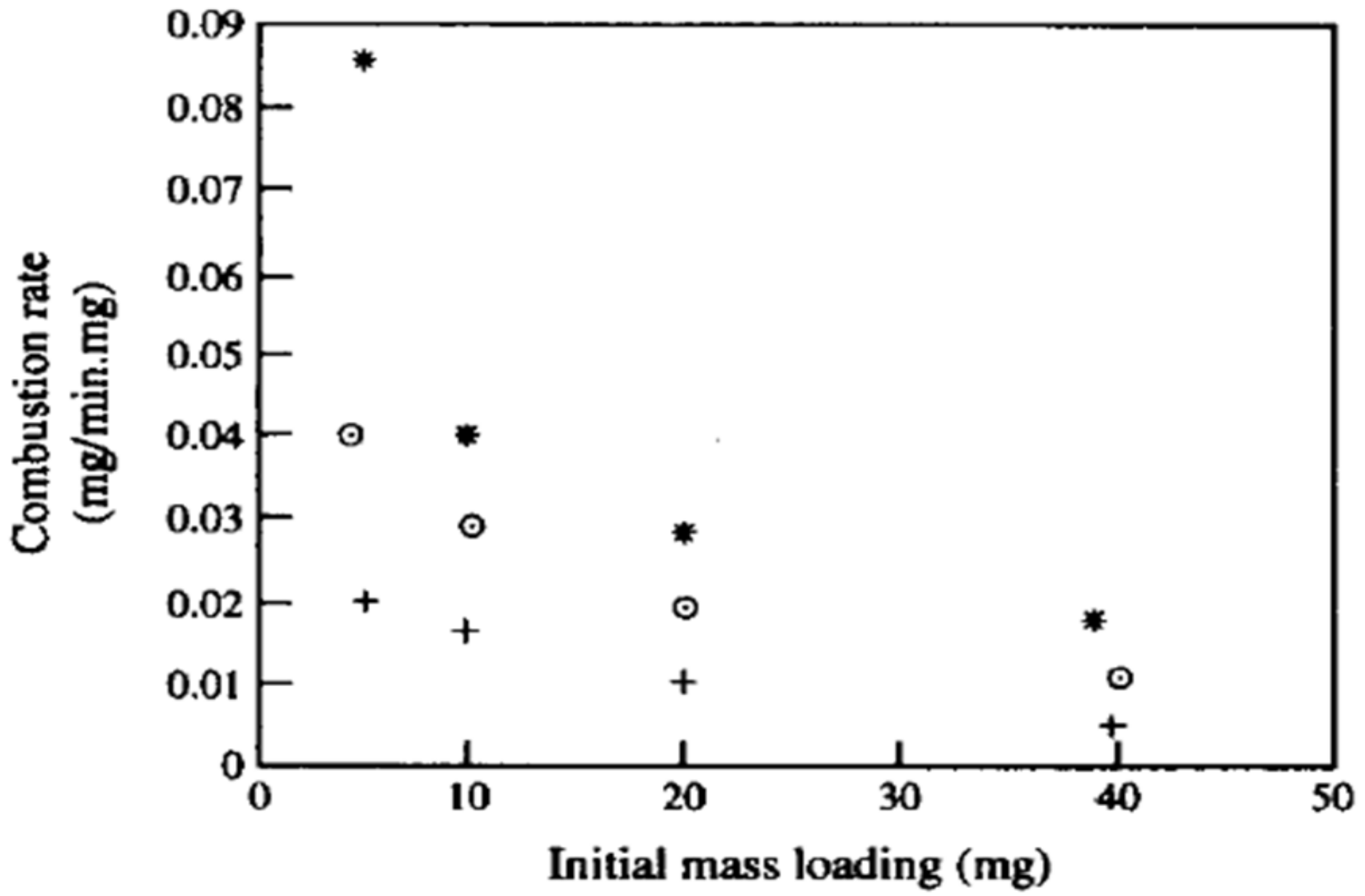
Gilot et al. [30] conducted experimental studies on the oxidation of black soot particles using a thermo-gravimetric analyzer (TGA) where a known amount of the sample (in mg) is exposed to an oxidizing atmosphere with a high temperature source of 600–900 °C. Mass versus time was measured. The specific combustion rate (g/s per g mass of cloud), or SERR, was found to decrease as the sample mass (or cloud size) is increased validating OD combustion model. Figure 4 shows the results with oxygen concentration as a parameter. The authors attribute the decreasing values of specific combustion rates to the limited diffusion of oxygen, which is consistent with the OD/GC modeling of dense clouds where the consumption rate of O₂, and hence the carbon burn rate (or O₂ consumption rate), decreases with increased sample or cloud mass.

2.3. Oxidation of Nutrients in BS

The macronutrients are typically CH and F. Oxygen, and water are rarely considered as nutrients [31]. Trayhurn, in his recent review [32] sets forth arguments that these are also nutrients, particularly when there is severe oxygen deficiency. However, water and oxygen are excluded as nutrients in the current review.

Just like oxidation of C(S) which occurs in two steps (Section 2.1), the oxidation of CH occurs in two steps: the first step is glycolysis of CH to pyruvate (an anaerobic process) outside of the mitochondria within cytoplasm of cells [33] and the second step is oxidation of pyruvate within mitochondria ((MITO, aerobic process). The benign cells derive 88% of energy from oxidation in Mito and 12% from glycolysis [34,35].

The oxygen in MITO serves as an electron accepter during oxidation.

ET (electron moles transferred per mole fuel) = 4 × (stoichiometric oxygen moles per mole fuel), assuming C to CO₂, H to H₂O, and S to SO₂ for oxidation of C_cH_hN_nO_oS_s fuels. For Glucose, ET = 24. As such, energy per electron mole is given by (1/4)*(HV_O2 in kJ/mole of O₂). Thus, the energy released per mole of electron for any C–H–O fuel is 454/4 = 115 kJ/mole of electron which is close to 111.1 as reported in [15]. The overall CH oxidation reaction is given as

C₆H₁₂O₆ + 6 O₂ + 36 ADP + 36 Pi + 6 O₂→6 CO₂ + 6 H₂O + 36 ATP,

On mass basis (excluding ATP, ADP, Pi),

0.94g of C₆H₁₂O₆ + 1 g of O₂ →1.38 g CO₂ + 0.56 g H₂O

Ref. [34] reports only 34 ATP per glucose molecule, and benign cells derive 88% of energy from oxidation and 12% from glycolysis [35]. On the other hand, cancer cells rely on glycolysis to provide most of the energy.

Energy Release Pathways: Depending on the local oxygen concentration and energy required, the cells can release energy through two pathways: (1). Oxidative phosphorylation (OXPHOS or Citric acid or Krebs cycle) is promoted by normal cells in the presence of “enough” oxygen level, which generate 36 ATP per glucose molecule. (2). The inefficient and more acidic glycolysis pathway to lactic acid is promoted when O₂ levels are deficient and generate only 2 ATP per glucose molecule resulting in a high lactate production [36], i.e., there is an augmentation of anerobic glycolysis under low p_O2. This is known as the Pasteur effects [37] where glucose consumption is increased in hypoxic conditions or when tumor or virus cells are present. The ERR is only about 12% of the energy from oxidation. The absence of mitochondria in cells (e.g., erythrocytes) can also lead to anerobic glycolysis as a major pathway for energy release.

2.4. Oxidation Models for Organs

Each organ contains billions of cells with a specific vital function, and they are irrigated by capillaries (micro-vasculature) with nutrients and O₂.

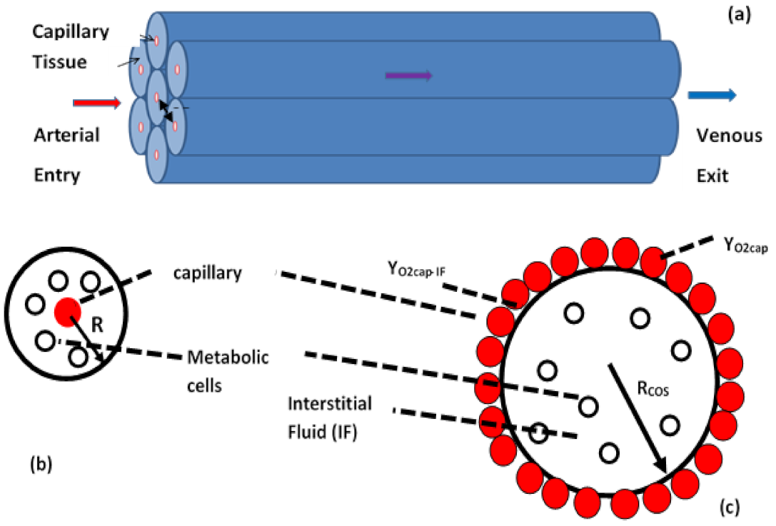
Oxidation Models for Organs: Oxidation of CH within each organ is modeled as though an organ is made up of a group of multiple cylinders of radii, R (Figure 5a) that contain metabolic cells supplied with oxygen from a capillary of radius r_cap at Y_O2cap located at the axis of each cylinder (Figure 5b). This model is known as the Krogh Cylinder model [38] and could be re-termed as the capillary on axis (COA) model. For a detailed review of Krogh models, see Ref. [39]. Each cylinder contains metabolic cells immersed in interstitial fluid (IF, the bulk phase in the cell cloud) (Figure 5c). Typically, the mixture in capillaries is CH rich and the oxidation is essentially controlled by diffusion of dissolved O₂ from capillaries to the IF and by the kinetics of oxidation within cells. Under kinetics control, Michaelis Menten kinetics are used for oxidation within MITO: C_Ch,k, is known for each organ; the constants depend on Michaelis Menten (MM) constants k_MM, in kinetics expression.

{\dot{w}}_{O 2, c e l l} = {\dot{w}}_{O 2, c e l l, \max} (\frac{Y_{O 2}}{Y_{O 2} + k_{M M}}), {\dot{w}}_{O 2, c e l l} \approx C_{C h, c e l l, k i n} Y_{O 2} w h e n Y_{O 2} < < k_{M M}, C_{C h, c e l l} = C_{C h, c e l l, k i n} = (\frac{{\dot{w}}_{O 2, c e l l, \max}}{k_{M M}})

(16)

Thus, first order kinetics is followed when Y_O2<<k_MM (or under OD condition). The model is like the “rich flammability limit” model in combustion science where the O₂ conservation equation is used to predict the rich flammability limit [40]. In addition to COA models, there are solid cylinder models where oxygen diffuses from the surface towards the core [41]. This has been re-termed as the capillaries on surface (COS) (Figure 5c) model.

The interface between IF and capillaries is at mass fraction of oxygen Y_O2cap-IF and will be the same as Y_O2cap if the mass transfer across capillaries is very fast. The COS model, or solid cylinder model in biology, is similar to the carbon dust cloud model used extensively in combustion science (see Figure 3) [26]. The cells of density, ρ_Cell, replace the density of carbon particles and the density of IF (density ρ_IF which is almost the same as ρ_Cel)) replaces the density of the bulk gas phase in the cloud combustion model. The Y_{O2, cl} at the carbon cloud surface (see Figure 3) is replaced by Y_O2cap-IF. In addition to the cylinder model, slab and spherical geometries are also considered for modeling the metabolism within an organ [42].

2.5. Oxygen Deficient Metabolism (ODM) in Organs

When an efficient vascular bed is absent, hypoxia occurs. The brain’s mass is only 2% of the total body mass but consumes 25% of the total oxygen for production of ATP for electrical activities [43] indicating high consumption rate of O₂ per unit mass of brain. More than 30% of COVID-19 patients have faced “brain fog” and impaired cognition. One of the major causes for this is a lack of oxygen or OD [44]. The tissue oxygenation level (typically p_O2 = 40–50 mm Hg, in some regions of the brain and as low as 16 mm Hg [32]) is hypoxic compared to alveoli levels (p_A,O2 = 104 mm Hg). Further, 50% saturation in arterial blood from lungs of COVID patients leads to an extremely rich mixture of CH and O₂, and the glycolysis pathway is promoted [45] under OD. About 44% of those recovered from COVID face neurological and psychiatric illnesses including delirium, seizures, encephalitis, etc. The studies by NYU School of Medicine found that the main culprit is low oxygen levels or OD in the organs of the body for extended periods of time [46].

The diffusional distance from the capillary for oxygen is about 100–200 μm. Those cells far from the capillary (e.g., the core of the cylinder in the COS model (Figure 5c) or the cells near the surface of the cylinder in COA model (Figure 5b)) may not receive oxygen, resulting in the cessation of oxidation. When the oxygen mass fraction falls below lethal levels,Y_{O2, leth} (somewhat like limiting oxygen index in combustion science), the oxidation reaction ceases, and cells rely more on glycolysis [37] for energy which generates more cell building ingredients. Thus, poorly oxygenated tissue or lethal parts of the tissue undergo glycolysis with an end product of lactic acid, which may lead to the destruction of healthy cells [47,48]. According to the Warburg hypothesis in biology, they also lead to the partial destruction of normal cells due to a reduced energy release and the creation of cancer cells [48].

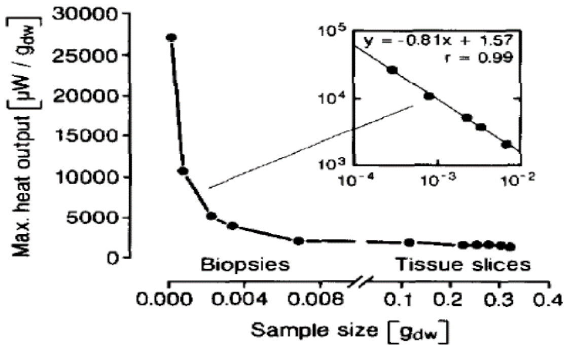
Singer et al. are probably the first in the field of biology to postulate the role of OD, or “crowding effect,” on the metabolic rates of in vitro (test tube) samples. They developed a phenomenological type of model [49] to explain the decrease of SMR_k with an increase in size of the in vitro sample. The model assumes (a) a spherical geometry of radius R, (b) a surface exposed to an O₂ rich atmosphere (similar to COS model), (c) a thin oxygenated (or aerobic) shell of thickness, δ (about 100 µm) near the surface, (d) a uniform source (US) model for O₂ consumption within the aerobic shell (R-δ < r < R) and (e) the anaerobic core (0 < r < R-δ) undergoing glycolysis. When the sample mass is small (m << 0.2g, R < δ), it is fully aerobic with Y_O2(r) ≈ Y_O2cap-IF everywhere; when the sample is large (about 0.2 g and higher or when R > δ), oxidation occurs at the outer shell with the core supplying only 5–10% of the oxidative energy release via glycolysis. If δ is assumed to be constant, then the aerobic volume fraction decreases for larger samples, which results in a lower SMR and validates the model with experimental data (Figure 6) [25] from in vitro samples.

2.6. Organ Mass Based Allometry (OMA)

It is apparent from the review of GC/OD literature from both fields that the SEER rates vary with cloud mass. However, the biology literature expresses the variation of SEER of organs (equivalent to the multiples of cell clouds) in terms of body mass using empirical allometric constants (Equation (7)). In order to compare these results with those from combustion science, the BMA for SERR of organs must be converted into organ mass based allometry (OMA) so that the allometric exponents can be interpreted in terms of OD deficient metabolism. Thus, eliminating m_B between Equations (7) and (8) [20]

{\dot{q}}_{k, m}, \{\frac{W a t t s}{k g o f o r g a n k}\} = E_{k} m_{k}^{F_{k}}, F_{k} = \{\frac{f_{k}}{d_{k}}\}, E_{k} = \{\frac{e_{k}}{c_{k}^{(\frac{f_{k}}{d_{k}})}}\}, k = K, H, B r, L, R

(17)

See Table 2 for F_k values based on 6 species and these will be re-presented in Section 5.5. It will be seen in Section 5.5 and Section 5.6 that the OD plays a major role in the allometric laws for the metabolic rates of vital organs and the whole body.

3. Objectives

The objectives of the current work are as follows: (i) extend the literature from OD combustion to OD metabolism including the transfer of the G number from combustion literature to G_OD number of each organ where OD represents oxygen deficiency, (ii) show that the local curve fitting of effectiveness factor (η_{eff, k}) vs. G_{OD, k} of an organ k leads to OMA and yields F_k values vs. G_OD,k, (iii) explain the negative exponents f_k and F_k of organs and show that

- \frac{1}{3} < F_{k} < 0

, (iv) validate the inequality with the experimental data for 6 and 111 species, (vi) explain and show that the negative exponents b’ of the whole body is affected by the size of the organ (or size of cell clouds) within BS and (vii) present the incipient G_OD,INC for organ k at which oxygen concentration reaches a lethal concentration in the core of the cell cloud resulting in a cessation of oxidation and the inception of glycolysis, a precursor to the creation of cancer cells. While a hypoxic condition for the whole body is given in terms of a saturation percentage in the arterial blood (≈92%) and (Hb) levels in blood, the manuscript presents G_{OD Inc} at the organ level, which is an indication for the onset of the hypoxic condition of an organ.

4. Materials and Methods

Governing Equations and Boundary Conditions for the ODM Model of Cell Clouds

Consider the spherical cloud of radius R and mass m_cl, containing n metabolic cells per unit volume of interstitial fluid (IF), with the cell cloud surface at Y_O2cap-IF (Figure 7).

Column 4, Table 3 presents the conservation equations, boundary conditions with and without lethal volume, and solutions for O₂ profiles. The spherical cell cloud mass, m_cl, of an organ k is assumed to be proportional to the organ’s mass, m_k, since an organ is modeled as a cluster of spherical cell clouds. The relation for oxygen consumption rate of a cell (

{\dot{w}}_{O 2, c e l l}

) located at r is given in row 1, column 4 of Table 3.

The cell within IF consumes oxygen either under diffusion control (O₂ transport rate << kinetics rate) or under first order kinetics control (kinetics rate << O₂ transport rate} (equations in row 1, column 4, Table 3). For example, C_ch,cell = 2 π d_cell (ρD)_eff [26] under diffusion control following the OD combustion literature. See Equation (16) for kinetics control. In both cases, the oxidation rate for the cell (

{\dot{w}}_{O 2, c e l l} (r)

) is proportional to the local oxygen mass fraction, Y_O2(r). Thus, the term C_{Ch, cell} changes when a cell metabolizes under kinetics control or diffusion control. The O₂ consumption rate per unit volume,

\dot{w}'''_{O 2} (r)

, is given as n

{\dot{w}}_{O 2, c e l l}

{row 4}. The conservation equations for oxygen species are given in dimensional form (row 4). The boundary conditions are given in row 7 with lethal volume, row 8 without lethal volume [26]; the (ρD) _eff, is called the effective mass diffusivity of O₂, which accounts for the presence of cells within the cloud.

Non-Dimensional G_OD Number for Organs and Physical Meaning: Following the combustion literature, the group number G_OD of cell clouds is defined as,

G_{O D, k} = {\{\frac{C_{c h, c e l l} n R^{2}}{{(ρ D)}_{e f f}}\}}_{k} = \frac{C h a r a c t r i s t i c O_{2} c o n s u m p t i o n r a t e b y a l l c e l l s w i t h i n c e l l l o u d}{C h a r a c t r i s t i c O_{2} d i f f u s i o n r a t e t o t h e c e l l s f r o m c a p i l l a r i e s},

(18)

The G_OD # is referred to as the OD number (row 6, column 3). When constant of proportionality C_Ch,cell is selected from the expression for kinetics-controlled metabolism, G_OD is same as (Thiele Modulus)². Higher G_OD numbers result in a higher oxygen deficiency within the cell cloud and the more the hypoxic condition of the organ, the more likely the cells are to adopt a glycolytic pathway for energy release. Both G and G_OD are proportional to R² ∝ m_cl^2/3 for dust clouds or m_k^2/3 for organ k. The conservation equations for oxygen species are given in non-dimensional form (row 5, non-dimensional radius, ξ = r/R) for dust clouds (column 3) and cell clouds (column 4) while row 6 defines the G# for dust clouds and G_OD # for applications to cell clouds in biology.

5. Results

5.1. Equilibrium Levels of Oxygen in Arterial Blood

The boundary condition for solution of conservation equations given in Table 3 require a knowledge of Y_O2,cap. The mass fractions of oxygen in capillaries of an organ k depends on the equilibrium mass fractions of oxygen (Y_O2,cap ≈ Y_O2,a) in the arterial blood. Hence the equilibrium levels of oxygen within arterial blood at partial pressure, p_a,O2, will be presented first. The Y_O2,a consists of two parts: dissolved O₂ and O₂ present as OHb. Based on the plot shown in Figure 2 (saturation % vs. p_O2, adopted and modified from ref. [12]) and data presented in the caption of Figure 2 shows the dissolved oxygen content in arterial blood can be plotted as a function of p_O2 (≈p_A,O2). The results for both the total and dissolved oxygen contents are shown in Figure 8. In COVID-19 patients, Hb denaturation occurs, thus reducing available (Hb)_in for oxidation to Hb (O₂) _in [45] and thus the transfer of oxygen across alveoli membrane to the capillary is disrupted, sometimes as low as 50% saturation (or saturation fraction = 0.5) of arterial blood. It also affects the transfer of CO₂ from blood to alveoli. The normal pH for humans is 7.35–7.45 and CO₂ loading reduces pH to 7.25, which increases the breathing rate.

5.2. Oxygen Profiles in Cell Clouds

Appendix A presents the solution for oxygen concentrations when the lethal volume is finite (Equations (A2) and (A3)). When ξ_leth is set to zero in Equation (A2), one recovers the solution for Y_O2 without lethal volume. The non-dimensional solutions for the oxygen mass fraction for carbon clouds and cell clouds are given in row 9 and 10 for cell clouds While O₂ mass fraction ranges around 300 ppm for healthy humans, the total Y_O2 could be as low 150 ppm and dissolved O₂ as low as 1.5 ppm at 50% saturation (Figure 8) for COVID-19 patients, indicating a very rich mixture of CH and O₂. Low O₂ concentration results in an increase of lethal volume within each vital organ. Detailed solutions for metabolic rates and extent of lethal volumes have been obtained for cell clouds involving slab, cylinder, and spherical geometries. However, the subsequent sections deal with presentations of solutions of a spherical cloud without lethal volume so that the methodology for deriving allometric laws of organs from effectiveness factor charts and validation of Kleiber’s law for the whole body can be kept in a tractable form. Figure 9 presents O₂ profiles with G (carbon clouds) or G_OD (cell clouds) as parameters. At low G_OD, the profile is almost flat, indicating a uniform O₂ consumption. They become steeper at high G_OD, indicating an aerobic shell of thickness δ near r = R while most of the inner cloud is anerobic.

5.3. Effectiveness Factor (η_eff)

Adopting the methodology used in combustion literature (e.g., porous char combustion), the results for O₂ profiles are used to determine the O₂ consumption rate for whole spherical clouds of radius R:

{\dot{w}}_{O 2} = n \int_{0}^{R} C_{c h, c e l l} Y_{O 2} (r) 4 π r^{2} d r, C e l l C l o u d

(19)

Defining the effectiveness factor, η_eff as [26,50]:

η_{e f f} = \frac{Y_{O 2, a v g}^{}}{Y_{O 2, c a p - I F}^{}} = \frac{O_{2} c o n s u m p t i o n r a t e b y a l l c e l l s w i t h i n c e l l c l o u d w i t h Y_{O 2} (r)}{O_{2} c o n s u m p t i o n r a t e b y a l l c e l l s w i t h i n c e l l c l o u d w i t h e a c h c e l l a t Y_{O 2} = Y_{O 2, c a p - I F}}

(20)

The numerator is proportional to the actual consumption rate, while the denominator is proportional to the hypothetical consumption rate when Y_O2 = Y_{O2, cap-IF} for all cells. Note that η_eff is only a function of G_OD for COS-O₂ models. Solutions for η_eff are given in row 13 of Table 3. The solutions for η_eff for the three geometries of cell clouds are the same as those from dust cloud literature [50]. Using results from combustion literature, Figure 10 presents the variation of η_eff with G_OD for the three geometries (See also equation in Table 3, row # 13). It is seen that effectiveness factors are close to each other under identical surface area to volume (S/V) ratios or similar surface area of capillaries to mass ratio, S_cap,m within organs.

Knowing G_OD, the η_eff is determined from Figure 10 and the oxygen consumption rate and hence the SMR_k oof any organ k can be estimated using Equation (21):

S M R_{k} (\frac{W}{k g}) = \frac{{\dot{w}}_{O 2, c l o u d} H V_{O 2}}{m_{c l o u d}} = {\dot{w}}_{O 2, m} H V_{O 2} = η_{e f f, k} \frac{C_{c h, c e l l} Y_{O 2, c a p - I F} n}{ρ} H V_{O 2}

(21)

5.4. Allometric Laws Derived from Effectiveness Factor Charts

The G_OD changes depending on the size of organ k of mass m_k and reactivity of cells within organ k. Large organs are typically at a high G_OD and small organs are at low G_OD. Thus, the solution for η_eff vs. G or G_OD,k presented in Table 3 (row # 13) can also be presented in the form of organ mass based allometric law using the following procedure.

For small intervals of G_OD (Figure 10) of any organ k, one can set:

η_{e f f, k} = A_{k} G_{O D}^{s_{k}}, k = B r, H, K, L

(22)

and determine the s_k values by curve fitting η_eff vs. G_OD,k and treating s_k as a constant for a narrow range of G_{OD, k}. Differentiating Equation (22) with G_OD,k (Figure 10),

\frac{d η_{e f f, k}}{d G_{O D, k}} = \frac{s_{k}}{G_{O D, k}}, k = B r, H, K, L

(23)

where

\frac{d η_{e f f, k}}{d G_{O D, k}}

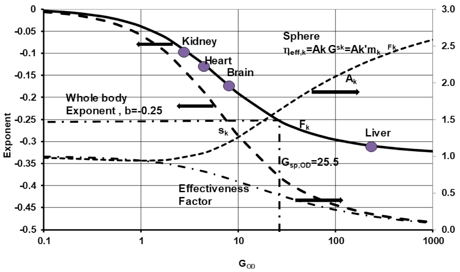
is obtained using the relation given for η_{eff, k,} with G_{OD, k} (row 13, Table 3). Using the result in Equation (23), the s_k values can be determined, plotting the results for s_k vs. G_{OD, k}. (Figure 11). Note that Figure 10 and hence Figure 12 are based on COS-O₂ model. The G`_{OD, k} ∝ m_k^(2/3), and hence

{\dot{q}}_{k, m} \propto η_{e f f, k} \propto G_{O D, k}^{s_{k}} \propto m_{k}^{(2 / 3) s_{k}}

. Comparing this with Equation (17),

F_{k} = \frac{2}{3} s_{k}, k = B r, H, K, L, COS- O_{2} model

(24)

The variation of F_k with G_{OD, k} is shown in Figure 11. All the F_k values are negative. As G_OD,k →0 (small organ), F_k → 0 and as G_OD,k →∞ (large organs), F_k→(−1/3). Hence, the F_k values satisfy the bounds:

- \frac{1}{3} < F_{k} < 0

for COS-O₂ models. While the phenomenological model of Singer with aerobic film of constant thickness and anaerobic core or lethal core [49] is used to explain the decrease of SMRk with an increase in size of the in vitro sample (equivalent to negative values for “f_k” coefficients used in the body mass based allometry), the current model assumes oxidation proceeding even at very low oxygen mass fraction within core, but still yields a decrease of SMR with an increase in size of the organ, More notably, it yields the bounds on “Fk” coefficients used in the organ mass based allometry

5.5. Validation with Experimental Data for Allometric Exponents

Effect of mass of organ-6 species: The organ masses were normalized with each kidney (K) mass (smallest mass). Using Equation (8), one can obtain normalized an allometric relation for m_k* which is a ratio of the organ mass to kidney mass.

m_{k} * = \frac{m_{k}}{m_{K}} = (\frac{c_{k, 6}}{c_{K, 6}}) m_{B}^{d_{k, 6} - d_{K, 6}} = g_{k, 6} m_{B}^{h_{k, 6}}, g_{k, 6} = (\frac{c_{k, 6}}{c_{K, 6}}), h_{k, 6} = d_{k, 6} - d_{K, 6}

(25)

where c_{k, 6} is the c_k value for organ k based on six species. Table 4 presents the values of g_{k, 6} and h_{k, 6.} The m_Br* ranges from 3.3–2.1, m_H* from 1.6 (0.48 kg rat) to 3.1 (65 kg human), and m_L* from 9.3–10.3, (row 3, Table 4) indicating a narrow variation, whereas the mass of the body ranged by a factor of 150. This is also apparent from Equation (25) where the values of |h_{k, 6}| are very low, and hence non-dimensional masses m_k*‘s are (row 3, Table 4) almost insensitive to variation in body mass.

Figure 12 shows the variation of the experimental exponent F_k with the variation of mk* for the six species (average value within square filled pattern). It is noted that the larger the organ mass, the more negative the value for F_k (indicating a higher OD). Based on the mean, the liver is larger with F_k near the theoretical limit of −0.33, while F_k is near zero for kidneys of smaller mass following the isometric law. Smaller organs are known to have faster O₂ delivery systems to the cells [23] since O₂ gradients are steeper. The metabolism of smaller organs, and hence smaller animals, may approach the maximum possible metabolic rate and thus they exhibit a lower tolerance to any environmental fluctuations.

Effect of mass of organ-111 species: Wang et al. [51] collected experimental data on the masses of vital organs of 111 species with body mass ranging from 0.0075 (shrew) to 6650 kg (elephant) (see Table A1 in Appendix B) and presented the following curve fit for the product of

{\dot{q}}_{k, m}

and m_k:

{\dot{q}}_{k} = {\dot{q}}_{k, m} x m_{k} = (e_{k, 6} m_{B}^{f_{k, 6}}) m_{k} = i_{k, 111} m_{B}^{j_{k, 111}}, k = B r, H, K, L

(26)

Values for i_k,111 and j_k,111 presented by Wang et al. for 111 species were adopted from [51] and are shown in rows 1 and 2 of Table 5. For

{\dot{q}}_{k, m}

, the authors of ref. [51] use e_k,6 and f_k,6 values (based on 6 species; see Table 2 and Table 4). By adding

({\dot{q}}_{k})

over all organ masses of 111 species, they verified Kleiber’s law (Equation (11)) and show that a = 3.21 W/(kg ^0.754), b = 0.754, and b’ = −0.246. However, allometric laws for the organ masses based on 111 species were not presented. Since Wang et al. used data on e_k,6 and f_k,6 for organ SMR_k, one can use the following relation to extract organ mass allometric coefficients c_k,111 and d_k,111.

{\dot{q}}_{k, m} x m_{k} = (e_{k, 6} m_{B}^{f_{k, 6}}) (c_{k, 111} m_{B}^{d_{k, 111}}) = i_{k, 111} m_{B}^{j_{k, 111}}, k = B r, H, K, L

(27)

The values for c_k,111 and d_{k, 111} are presented in rows 3 and 4 of Table 5 and values for c_k,6 and d_k,6 are provided in parentheses in the same table for comparison. See Table A1 in the Appendix for the data table for the masses of organs of 111 species tabulated in ref. [51]. The normalized organ mass relation for 111 species is given as:

m_{k} * = \frac{m_{k}}{m_{K}} = (\frac{c_{k, 111}}{c_{K, 111}}) m_{B}^{d_{k, 111} - d_{K, 111}} = g_{k, 111} m_{B}^{h 111}, g_{k, 111} = (\frac{c_{k, 111}}{c_{K, 111}}), h_{k, 111} = d_{k, 111} - d_{K, 111}

(28)

Note that h_{k, 111} (= d_k,111 − d_K_,111) is extremely low for vital organs indicating a narrow variation in m_k*. Hence the variation in m_k* is extremely small when the body mass changed by a factor of 900,000. The F_k values remain almost unchanged (row 5, Table 5). The values c_{k, 111} compared to c_{k, 6} and d_k,111 compared to d_k,6 are not much different.

Effect of Geometry: The results presented for F_k vs. m_k* (Figure 11) are based on spherical geometry. Rather, if the Krogh cylinder model is adopted for the same S_{cap, m} (same capillary surface area to mass ratio) it is equivalent to the same S/V ratio (=S_{cap, m}*ρ). As seen in Figure 10, the effectiveness factors are close to each other for these geometries and hence, for F_k, or S_{cap, m}, the values will not differ much from each other.

5.6. Whole Body Allometric Law for Metabolic Rate

Various approaches have been undertaken to validate Kleiber’s law: surface area rule, oxygen consumption, and capillary surface area rule [52], heterogeneous model of Wang, etc. [17]. (See review in [53]).

If one assumes that all organs within the body are equally larger sized, then Kleiber’s law for the whole body will yield F_k = b’ = −1/3. Similarly, if all organs are extremely small or equally small, then F_k = 0 (Figure 11), and Kleiber’s law for the whole body will yield F_k = b’ = 0. However, a BS contains organs of different sizes and hence the exponent b’ = −1/4 must satisfy the inequality −1/3 < b’ < 0 if organ sizes vary from smaller to larger. Wang et al. summed up metabolic contribution by five significant organs (Br, H, K, L and R) within the body (Equation (7)) using f_k values based on body mass or F_k values based on organ mass, obtained Kleiber’s law with b’= −1/4, which satisfies the above inequality [17]. The relation between F_k and organ mass m_k leads to Kleiber’s law for the whole body. It appears that the” Kleiber’s Law or the 3/4 Rule may neither be a law nor a Rule” [53] but appears to be consequence of combined contributions from all organs of various sizes with different effectiveness factors or oxidation at different concentrations of O₂.

5.7. G_OD Number Estimation of Vital Organs

The definition of G_OD,k can be used to estimate the G_OD,k, the number for vital organs, if the constant of proportionality, C_Ch,k, is known for each organ; the constants depend on Michaelis Menten (MM) constants k_MM in kinetics expression (Equation (16))

{\dot{w}}_{O 2, c e l l} = {\dot{w}}_{O 2, c e l l, \max} (\frac{Y_{O 2}}{Y_{O 2} + k_{M M}})

(29)

for each organ if kinetics control and effective diffusivity if diffusion control. On the other hand, if the experimental data for F_k is known, the corresponding G_{OD, k} can be determined using Figure 11. Since F_k is close to the lower limit of −0.333, the liver, the largest vital organ, has the highest G_OD number (=Thiele Modulus²), while the kidney has the lowest values. The same figure shows the allometric exponent for the whole body (Figure 11) and hence, for the six species considered (0.48–65 kg body mass), the BS operates with an overall G_OD of 26 and effectiveness factor of 0.48 (i.e., oxidation for whole body is at 48 % capillary oxygen concentration) for spherical geometry which is close to ψ_T² = 25 (presented in the Appendix of Ref. [54]). Note that [54] uses the whole-body approach and the Thiele modulus in modeling the metabolism. While Thiele modulus is typically used when cells in cell cloud consume oxygen under first order kinetics control, the G_OD as defined here is more general and can be used for kinetics control (for which G# = Ψ_T², ref. [26,29]), diffusion, or combined control.

5.8. Incipient ODC or Group Combustion and Incipient ODM

The incipient combustion number, G_INC, is transferred from the combustion literature to incipient number, G_{OD, INC}, for organs where oxygen concentration reaches “extinction” levels at the core of cell clouds resulting in cessation of oxidation and the inception of fermentation, a precursor to the creation of cancer cells. Cancer cells rely more on glycolysis (which produces ingredients for growth of new cells) due to mitochondrial impairment and oxygen deficiency [55].

As the number of cells per unit volume (n) is increased or when the enzyme activity is enhanced, there is an increasing amount of consumption of oxygen by cells closer to capillaries which lowers the oxygen concentration at the core (r = 0). At G_{OD, Inc,} the Y_O2 at r = 0 reaches the lethal mass fraction Y_{O2, lethal} (about 1 ppm) below which the cells in the core undergo only glycolysis. This condition for cell clouds is like the extinction condition in combustion literature and G_INC at this condition is termed as the incipient group combustion in combustion literature. Table 3 row 12 presents the relation for G_{OD, Inc}. At G_{OD, INC,} the cells at the core become oxygen deficient and the oxidation reaction ceases. For example, if Y_O2leth/Y_O2cap-IF is set at 0.2, then G_{OD, INC} = 10. Note that oxygen deficiency is one of the causes for creation of cancer cells but not necessarily the cause. Tumor cells seem to adopt glycolysis as a metabolic pathway for energy conversion independent of oxygen levels within the cells. Thus, one may chronologically monitor the G_OD# of each organ and if it keeps increasing over a period, there is a likelihood of the formation of cancer cells.

According to the present hypothesis, a larger species is more likely to develop cancer, although there is some existing evidence to the contrary [56]. On the other hand, a large organ like the liver can afford impairment, while small organs like the pancreas cannot and they could be compromised with only a few tumor cells [57]. Further, the present hypothesis does not consider the fact that a reduced metabolic rate reduces the number of electrons transferred which reduces the oxygen radical concentration resulting in a reduced oncogenic mutation and hence a reduced rate of buildup of cancer cells [56]. Thus, the competitive effects seem to be present in each generation of cancer cells. Typically, the highest rate of cancer occurs in the breast followed by lung cancer and prostate. The future work should track G_OD,k for these organs for any sign of gradual increase in G_OD,k. Similarly, in COVID-19 patients with 50% saturation in arterial blood, the location of Y_O2leth is close to the capillaries on the surface, leaving a large anerobic core or lethal volume with reduced ATP production and resulting in the loss of vital functions.

6. Conclusions

The dimensionless number (G) used in combustion science was modified to G_OD for the application to OD metabolisms in organs.
The rationale for negative exponents (F_k) in the allometric law for SMR of vital organs, ${\dot{q}}_{k, m} \propto m_{k}^{F_{k}}$ , is provided through the adoption of group combustion or OD theory from combustion science within biology. The exponent F_k satisfies the inequality $- \frac{1}{3} < F_{k} < 0$ for COS-O₂ model. Thus, the allometric law for an organ is shown to be an empirical approximation of effectiveness chart.
The negative exponent b’ in the allometric law for the SMR of the whole body satisfies the inequality $- \frac{1}{3} < b' < 0$ with b’ = −1/4 (Kleiber’s law). The negative exponent b’ = −1/4 is due to distributed sizes of various organs with differing values for F_k.
Based on experimental data from F_k, the G_OD numbers were estimated for vital organs as 2.8, 4.2, 9, and 240 for the kidney, heart, brain, and liver, respectively. The average G_OD for the whole body of all BS with an equivalent organ is about 26 with effectiveness factor of 0.48 (i.e., oxidation of all tissues at 48% capillary oxygen concentration), considering spherical geometries for cell clouds.
While the hypoxic condition of the whole body is characterized by the saturation percentage, the introduction of the G_OD number characterizes OD at organ level.
Glycolysis is inhibited when there is a high level of ATP within cells and vice versa; thus, reduced O₂ concentration results in a reduced ERR per unit volume which results in reduced ATP concentration, which promotes glycolysis pathway [58,59]. Cancer and virus cells, including those of COVID-19 patients, rely on the glycolysis pathway to provide the building blocks for uncontrollable cell growth.

Funding

The seeds for the research on group/oxygen-deficient combustion of carbon clouds were planted by the earlier funding from DOE-Pittsburgh: DE-FG22-90 PC 90310. DE-FG 22-88 PC 88937, DE-FG 22-85 PC 80528 and Department of Energy—Morgantown: DOE-METC DE-AC21-86 MC 23256. The current research was initiated after observing the similarity of the results on energy release rate from carbon clouds with those from organs (cell clouds). The author wishes to acknowledge the partial support of the research funds from Paul Pepper Professorship.

Institutional Review Board Statement

Not applicable.

Informed Consent Statement

Not applicable.

Data Availability Statement

Not applicable.

Acknowledgments

Vishal M. Gohil, Biochemistry and Biophysics, Texas A&M University, for fruitful discussions on mitochondria and metabolism. Mathew Miller, for help in generating Hb-O₂ equilibrium curves and Figure 5 and Figure 7. Megan Simpson of the Department of Mechanical Engineering, Texas A&M University, for English editing of manuscript.

Conflicts of Interest

The author declares no conflict of interest.

Abbreviations/Nomenclature

Nomenclature
A_k	see Equation (22), pre-exponential factor
a, b, b’	allometric coefficients for metabolism
C_{ch, cell}	Characteristic Oxygen Consumption Rate for cell, g/s, {Table 3}
C_{ch, p}	Characteristic Oxygen Consumption Rate for carbon particle, g/s, {Table 3}
ck	pre-exponent in the allometry relation for mass of organ
D	Diffusivity, cm²/s
D_eff	Effective Diffusion Coefficient, cm²/s
d_cell	Diameter of cell, cm
d_k	exponent in allometry relation for mass of organ
d_p	Diameter of particle, cm
D	Diffusion Coefficient of Molecular Oxygen
D_eff	Effective diffusion Coefficient
e_k	pre-exponent in the allometry relation for metabolic rate
F_k	Allometric exponent, organ mass based { ${\dot{q}}_{k, m} = E_{k} m_{k}^{F_{k}}$ }
f_k	Allometric exponent, body mass based allometry used in ${\dot{q}}_{k, m} = e_{k} m_{B}^{f_{k}}$ }
G	Group combustion number in combustion science {Table 3}
G_OD	Group metabolism number in biology to indicate extent of Oxygen Deficiency (OD)
G_{OD, kin}	Group metabolism number for organ k under kinetics control {= Ψ_T² or Thiele Modulus², $\{\propto R_{k}^{}^{2} \propto m_{k^{2 / 3}}\}$
G_{k, OD, diff}	Group metabolism number for organ k under diffusion control, $\{\propto R_{k}^{}^{2} \propto m_{k^{2 / 3}}\}$
g_k, h_k	see Equation (25)
(Hb)	Hemoglobin concentration on mass basis, g per DL of blood
[Hb]	Hemoglobin concentration on mole basis, moles per DL of blood
H_O2	Henry’s constant for solubility of O₂ in blood
HV	Heating Value of fuel or nutrient, J/g fuel
HV_O2	Heating Value per unit mass of O₂ consumed, J/g O₂
J_k	Pre-exponent in allometry relation for OEF
k_MM	Constant in MM kinetics, Equation (29), = Y_O2 at half of maximum metabolic rate
K_n’	Equilibrium Constant, (1/mm Hg when n = 1, 1/mm Hg² n = 2, etc.), n = 1, 2, 3, 4
L_MM	Constant in LM kinetics, Y_O2 at half of maximum oxygen consumption rate ${\dot{w}}_{O 2, p, \max}$
m_B	Body mass, kg
m_cl	cloud mass, kg
mk,	k th organ mass, kg, Brain, Heart, Kidney, liver etc.
mk*	Non-dimensional mass, = {mass of organ k/Mass of kidney}
n	number of particle or cells per unit volume, particles/cm³, or cells/cm³
p_O2	Partial pressure of O₂, mm of Hg
$\dot{Q}$	Energy released in the form of heat, W
$\dot{q}$	Energy release rate (ERR) or metabolic rate, W
$\dot{q}$ k, _m	Specific Energy Release Rate or SMR (SERR), W/kg of k-th organ
$\dot{q}$ _m	Specific Energy Release Rate or SMR (SERR), W/kg
r	radius
r_cap	Capillary radius, cm
R, R_cl	Cloud radius, cm
RQ	Respiratory Quotient, =CO₂ moles/O₂ moles, Table 1
S, S_cap	Capillary surface area, cm²
S_{cap, m}	Specific capillary surface area based on mass, cm²/g of tissue, {=S/ (ρ V)}
s_k	See equation (22), exponent
V	Volume, = cm³
$\dot{W}, {\dot{W}}_{A T P}$	Energy Released in the form of Work or ATP, W
${\dot{w}}_{O 2}, {\dot{w}}_{O 2}'', {\dot{w}}_{O 2}'''$	Oxygen Consumption rate, g/s; per unit area, g/(cm² s), per unit volume, g/(cm³ s)
Y_O2	Mass fraction of oxygen, (g of O₂/g of mixture)
δ	Aerobic shell thickness
Greek Symbols
ξ	Non-dimensional radius, r/R
ρ_bl	Density of blood, g/cm³
ψ_T	Thiele Modulus, $\sqrt{G_{k i n}} o r \sqrt{G_{O D, k i n}}$
η_eff	Effectiveness factor based on capillary-IF interface O₂ concentration, = Y_{O2, avg}/Y_{O2, cap-IF}
η_M	metabolic efficiency
ν_O2	stoichiometric Oxygen
Subscripts
A	Alveolar
avg	Average
a	Arterial
B	Body
Bl	Blood
cap	capillary
Cap-IF	interface between capillary and Interstitial Fluid (IF)
cl	Cloud
eff	effective
ext	extinction
IF	Interstitial fluid
k	organ k, Brain (Br), Heart (H), Kidney (K), liver (L) etc.
Leth	Lethal
m	per unit mass
O₂	oxygen
Abbreviations
ATP	Adenosine triphosphate
BMA	Body mass based allometry
Br, H, K, L, R	Brain, Heart, Kidney, Liver, Residual
BS	Biological systems
CH	Carbo-hydrate, e.g., glucose
COA	Capillary on Axis of Cylinder
COS	Capillary on Surface of Cylinder or solid cylinder model
ER	Equivalence radio in engineering, O₂ used/O₂ supplied, ER < 1 dilute mix
ERR	Energy Release Rate, W
F	Fat
GC	Group Combustion
ICD	Inter-capillary Distance, cm
IF	Interstitial Fluid
Iso	isolated
LM	Langmuir kinetics
MITO	Mitochondria
MM	Michaelis Menton kinetics
MR	Metabolic rate, W
OD	Oxygen Deficiency, oxygen deficient
ODC	Oxygen Deficient Combustion
ODM	Oxygen deficient metabolism
OEF	Oxygen Extraction Fraction (g O₂ extracted for metabolism er g O in blood = Equivalence Ratio in Combustion. Science for dilute Combustible Mix)
OHb	Oxy-Hemoglobin
OMA	Organ mass based allometry
OXPHOS	Oxidative phosphorylation
P	Protein
ppm	parts per million {(g per/g blood) * 10⁶}
RBC	Red Blood Cells
Sa	Saturation
SERR	Specific Energy Release Rate, W/g
SERR_M	Specific Energy Release Rate, W/g body mass
SMRk	Specific Metabolic Rate (term in Biology for SERR) of organ k, W/g
SMR_M	Specific Metabolic Rate of whole body, W/g body mass

Appendix A. Solutions for Oxygen Concentrations with Lethal Volume

Consider

\frac{d^{2} Y_{O 2}}{d ξ^{2}} + (\frac{2}{ξ}) \frac{d Y_{O 2}}{d ξ} = Y_{O 2} G_{O D}

(A1)

Using the boundary conditions Y_{O2 =} Y_{O2, ccap-IF at} ξ = 1 and dY_O2/dξ = 0 at ξ = ξ_leth. The solution for Y_O2 with lethal volume is given as

\frac{Y_{O 2} (ξ)}{Y_{O 2}_{c a p - I F}} = \frac{[\frac{S i n h (\sqrt{G_{O D}} ξ)}{\sqrt{G_{O D}} ξ} - \frac{{\sqrt{G_{O D}} ξ_{l e t h} - t a n h (\sqrt{G_{O D}} ξ_{l e t h})}}{{\sqrt{G_{O D}} t a n h (\sqrt{G_{O D}} ξ_{l e t h}) - 1}} \frac{\cosh (\sqrt{G_{O D}} ξ)}{\sqrt{G_{O D}} ξ}]}{{\frac{S i n h (\sqrt{G_{O D}})}{\sqrt{G_{O D}}} - \frac{{\sqrt{G_{O D}} ξ_{l e t h} - t a n h (\sqrt{G_{O D}} ξ_{l e t h})}}{{\sqrt{G_{O D}} ξ_{l e t h} t a n h (\sqrt{G_{O D}} ξ_{l e t h}) - 1}} \frac{c o s h (\sqrt{G_{O D}})}{\sqrt{G_{O D}}}}}, COS- O_{2}, L e t h a l

(A2)

where ξ_leth can be solved by setting Y_O2 = Y_{O2 leth} at ξ= ξ_leth

\frac{Y_{O 2, l e t h}}{Y_{O 2}_{c a p - I F}} = \frac{[\frac{S i n h (\sqrt{G_{O D}} ξ_{l e t h})}{\sqrt{G_{O D}} ξ_{l e t h}} - - \frac{{\sqrt{G_{O D}} ξ_{l e t h} - t a n h (\sqrt{G_{O D}} ξ_{l e t h})}}{{\sqrt{G_{O D}} t a n h (\sqrt{G_{O D}} ξ_{l e t h}) - 1}} \frac{\cosh (\sqrt{G_{O D}} ξ_{l e t h})}{\sqrt{G_{O D}} ξ_{l e t h}}]}{{- \frac{{\sqrt{G_{O D}} ξ_{l e t h} - t a n h (\sqrt{G_{O D}} ξ_{l e t h})}}{{\sqrt{G_{O D}} ξ_{l e t h} t a n h (\sqrt{G_{O D}} ξ_{l e t h}) - 1}} \frac{c o s h (\sqrt{G_{O D}})}{\sqrt{G_{O D}}} + \frac{S i n h (\sqrt{G_{O D}})}{\sqrt{G_{O D}}}}}, COS- O_{2}, L e t h a l

(A3)

By letting ξ_leth = 0, (i.e., solution with no lethal volume), Equation (A2) becomes

\frac{Y_{O 2} (ξ)}{Y_{O 2}_{c a p - I F}} = \frac{1}{ξ} [\frac{S i n h (\sqrt{G_{O D}} ξ)}{S i n h (\sqrt{G_{O D}})}], COS- O_{2}, N o L e t h a l v o l

(A4)

which is the same as the solution presented in row 10 of Table 3.

Appendix B. Collected Organ Mass and Metabolism Data On 111 Species

Table A1. Data on organ mass in kg, normalized mass and specific metabolic rates of vital organs and computed overall metabolic rate of whole body for 111 species. Mass and specific metabolic rate data for organs and whole body adopted from [51] and specific metabolic rate of organs (SMR) converted into Watts. Normalized organ mass {m_k* = m_k/m_K} computed in current manuscript. q_k,m (SMR) W/kg, k = L, Br, H, K and R; q_Het: Metabolic rate of whole body-Heterogeneous approach, W; q_Het,m: Specific Metabolic rate of whole body-Heterogeneous approach, W/kg. m_B = m_L + m_Br + m_H + m_K + m_R.

Species	M	q_L,m	q_Br,m	q_H,m	q_K,m	q_R,m	m_L	m_Br	m_H	m_K	m_R	q _Het,	q _Het,m	m_L *	m_Br *	m_H *
Sorex araneus	0.0075	123	43	77	50	3	0.00038	0.00015	0.00011	0.00011	0.0068	0.09	11.86	6.91	2.73	2.00
Crocidura russula	0.0100	115	42	75	49	3	0.00055	0.00017	0.00008	0.00013	0.0086	0.10	10.85	8.46	2.62	1.23
Lasiurus borealis	0.0140	105	40	72	48	3	0.00035	0.00017	0.00014	0.00011	0.013	0.10	7.17	6.36	3.09	2.55
Lasionycteris noctivagans	0.0150	102	39	71	47	3	0.00033	0.00016	0.00016	0.00013	0.014	0.10	6.68	5.08	2.46	2.46
Mus musculus	0.0150	102	39	71	47	3	0.00068	0.00036	0.00007	0.00028	0.014	0.14	9.49	4.86	2.57	0.50
Myodes glareolus	0.0150	101	39	71	47	3	0.00067	0.00035	0.0001	0.00024	0.014	0.14	9.10	5.58	2.92	0.83
Microtus agrestis	0.0150	101	39	71	47	3	0.00063	0.00039	0.00012	0.00017	0.014	0.14	8.86	7.41	4.59	1.41
Neomys fodiens	0.0160	101	39	70	47	3	0.00055	0.00025	0.00014	0.00022	0.015	0.13	8.14	5.00	2.27	1.27
Blarina brevicauda	0.0180	97	38	69	47	3	0.00093	0.00032	0.00018	0.00021	0.016	0.17	9.64	8.86	3.05	1.71
Apodemus sylvaticus	0.0180	97	38	69	47	3	0.0011	0.00057	0.00014	0.00026	0.016	0.19	10.70	8.46	4.38	1.08
Microtus	0.0210	93	37	68	46	3	0.0011	0.00058	0.00015	0.00036	0.019	0.19	8.91	6.11	3.22	0.83
Peromyscus leucopus	0.0220	92	37	68	46	3	0.0012	0.00074	0.00015	0.0003	0.02	0.22	9.88	8.00	4.93	1.00
Apodemus flavicollis	0.0250	89	37	67	45	3	0.001	0.00061	0.00018	0.00034	0.023	0.20	7.94	5.88	3.59	1.06
Nyctalus noctula	0.0260	88	36	66	45	3	0.0005	0.00032	0.00037	0.00013	0.024	0.15	5.76	7.69	4.92	5.69
Microtus arvalis	0.0270	87	36	66	45	3	0.0019	0.00039	0.00019	0.00055	0.024	0.28	10.31	6.91	1.42	0.69
Mouse	0.0280	86	36	66	45	3	0.0018	0.0005	0.00016	0.00051	0.025	0.27	9.64	7.06	1.96	0.63
Gerbillus perpallidus	0.0300	85	36	65	45	3	0.001	0.00058	0.00013	0.00027	0.028	0.19	6.54	7.41	4.30	0.96
Mustela nivalis	0.0320	83	35	65	44	3	0.0016	0.0018	0.00036	0.00043	0.028	0.31	9.49	7.44	8.37	1.67
Acomys minous	0.0420	77	34	63	43	2	0.0009	0.0009	0.00018	0.00032	0.04	0.23	5.33	5.63	5.63	1.13
Jaculus jaculus	0.0480	75	33	62	43	2	0.0011	0.0012	0.00045	0.00029	0.045	0.27	5.67	7.59	8.28	3.10
Rhabdomys pumilio	0.0500	74	33	61	43	2	0.0018	0.0006	0.00021	0.00041	0.047	5.96	0.00	8.78	2.93	1.02
Talpa europaea	0.0510	73	33	61	43	2	0.0015	0.001	0.00031	0.00036	0.048	0.30	5.71	8.33	5.56	1.72
Glaucomys volans	0.0550	72	33	61	43	2	0.0029	0.0019	0.00056	0.00059	0.049	0.45	8.09	9.83	6.44	1.90
Arvicola terrestris	0.0620	70	32	60	42	2	0.0026	0.0011	0.00028	0.0007	0.057	0.39	6.34	7.43	3.14	0.80
Glis glis	0.0830	64	31	58	41	2	0.0032	0.0015	0.00048	0.00068	0.078	0.48	5.71	9.41	4.41	1.41
Tamias striatus	0.1040	61	30	56	40	2	0.0029	0.0024	0.00066	0.00081	0.097	5.04	0.00	7.16	5.93	1.63
Octodon degus	0.1290	57	29	55	40	2	0.0048	0.0019	0.00041	0.0011	0.121	4.99	0.00	8.73	3.45	0.75
Tupaia glis	0.1410	56	29	54	39	2	0.0034	0.0034	0.00117	0.0011	0.132	4.69	0.00	6.18	6.18	2.13
Rat	0.1500	55	28	54	39	2	0.0092	0.0023	0.0007	0.0014	0.136	6.25	0.00	13.1	3.29	1.00
Cebuella	0.1630	54	28	53	39	2	0.0135	0.0044	0.00086	0.0019	0.142	1.25	0.00	14.2	4.63	0.91
Rattus norvegicus	0.2100	50	27	52	38	2	0.0092	0.0023	0.00087	0.0015	0.196	4.75	0.00	12.3	3.07	1.16
Cheirogaleus medius	0.2310	49	27	51	38	2	0.0063	0.0028	0.00093	0.001	0.22	3.80	0.00	12.6	5.60	1.86
Rat	0.2500	48	26	51	37	2	0.012	0.002	0.00094	0.0021	0.233	4.73	0.00	11.4	1.90	0.90
Mustela erminea	0.2590	48	26	51	37	2	0.01	0.0057	0.0025	0.0023	0.238	4.89	0.00	8.70	4.96	2.17
Helogale parvula	0.2600	48	26	51	37	2	0.0111	0.0052	0.0015	0.0025	0.24	4.84	0.00	8.88	4.16	1.20
Sciurus vulgaris	0.2750	47	26	50	37	2	0.0055	0.0063	0.0017	0.0017	0.259	3.77	0.00	6.47	7.41	2.00
Callithrix jacchus	0.3120	45	26	49	37	2	0.0178	0.0073	0.0028	0.0029	0.281	5.57	0.00	12.3	5.03	1.93
Saguinus fuscicollis	0.3300	45	25	49	37	2	0.0144	0.0078	0.0033	0.0019	0.303	1.60	0.00	15.2	8.21	3.47
Rat	0.3370	44	25	49	37	2	0.008	0.0019	0.001	0.0023	0.324	1.10	0.00	6.96	1.65	0.87
Rat (Wistar)	0.3900	43	25	48	36	2	0.0143	0.0019	0.0011	0.0028	0.37	1.44	0.00	10.2	1.36	0.79
Sciurus niger	0.4120	42	25	48	36	2	0.0107	0.0075	0.0025	0.003	0.389	1.52	0.00	7.13	5.00	1.67
Sciurus carolinensis	0.5960	38	23	46	35	2	0.0164	0.0075	0.0028	0.0032	0.566	1.94	0.00	10.3	4.69	1.75
Saguinus oedipus	0.6240	38	23	46	35	2	0.0209	0.01	0.0037	0.0031	0.586	2.21	0.00	13.5	6.45	2.39
Mustela putorius	0.6400	37	23	45	35	2	0.0288	0.0104	0.0048	0.004	0.592	2.60	4.06	14.4	5.20	2.40
Leontopithecus chrysomelas	0.6420	37	23	45	35	2	0.0189	0.0132	0.0038	0.0041	0.602	2.27	3.54	9.22	6.44	1.85
Guinea pig	0.8000	35	22	44	34	2	0.027	0.0047	0.0023	0.0056	0.76	2.49	3.11	9.64	1.68	0.82
Potorous tridactylu	0.8090	35	22	44	34	2	0.0237	0.0114	0.0048	0.0062	0.763	2.65	3.28	7.65	3.68	1.55
Erinaceus europaeus	0.9500	34	22	43	34	1	0.0496	0.0043	0.0055	0.0089	0.881	3.59	3.78	11.2	0.97	1.24
Sylvilagus floridanus	0.9720	33	22	43	33	1	0.032	0.0079	0.0048	0.0063	0.921	3.00	3.08	10.2	2.51	1.52
Ondatra zibethicus	0.9910	33	22	43	33	1	0.026	0.0047	0.003	0.0058	0.952	2.67	2.69	8.97	1.62	1.03
Saimiri boliviensis	1.0000	33	22	43	33	1	0.0194	0.029	0.0065	0.0067	0.941	3.14	3.13	5.79	8.66	1.94
Martes foina	1.4100	30	21	41	32	1	0.0349	0.019	0.0098	0.0073	1.335	3.92	2.79	9.56	5.21	2.68
Mephitis	1.4500	30	21	41	32	1	0.0174	0.0098	0.006	0.0066	1.409	3.11	2.15	5.27	2.97	1.82
Trichosurus vulpecula	1.5500	29	20	41	32	1	0.0332	0.0127	0.009	0.0135	1.482	4.03	2.60	4.92	1.88	1.33
Martes martes	1.6000	29	20	41	32	1	0.0379	0.0205	0.0108	0.0088	1.525	4.29	2.68	8.61	4.66	2.45
Cebus apella	1.7500	29	20	40	32	1	0.0493	0.0508	0.0134	0.0104	1.626	5.42	3.11	9.48	9.77	2.58
Eulemur macaco macaco	1.8800	28	20	40	32	1	0.0778	0.0242	0.0091	0.0142	1.75	5.76	3.07	10.9	3.41	1.28
Chrotagale owstoni	1.9600	28	20	40	32	1	0.0441	0.0233	0.0116	0.0128	1.868	4.99	2.53	6.89	3.64	1.81
Vulpes corsac	2.0800	27	20	40	31	1	0.0356	0.0341	0.0217	0.0088	1.975	5.33	2.56	8.09	7.75	4.93
Lemur catta	2.0800	27	20	40	31	1	0.0729	0.0228	0.0117	0.0112	1.956	5.76	2.77	13.0	4.07	2.09
Eulemur fulvus fulvus	2.5000	26	19	39	31	1	0.0434	0.0225	0.0118	0.0095	2.413	5.33	2.12	9.14	4.74	2.48
Felis silvestris	2.5700	26	19	39	31	1	0.0502	0.0381	0.0103	0.0154	2.459	5.91	2.31	6.52	4.95	1.34
Didelphis virginiana	2.6300	26	19	38	31	1	0.1573	0.0083	0.0121	0.0229	2.433	8.33	3.17	13.7	0.72	1.06
Aonyx cinerea	2.6800	25	19	38	31	1	0.1064	0.0359	0.0151	0.0306	2.487	7.99	2.98	6.95	2.35	0.99
Leopardus geoffroyi	3.1000	24	18	38	30	1	0.0584	0.0321	0.016	0.0307	2.963	7.12	2.30	3.80	2.09	1.04
Lepus europaeus	3.3400	24	18	37	30	1	0.0904	0.0148	0.0289	0.0185	3.186	7.85	2.35	9.77	1.60	3.12
Dasyprocta punctata	3.4000	24	18	37	30	1	0.1088	0.0228	0.0363	0.0213	3.211	8.81	2.59	10.2	2.14	3.41
Potos flavus	3.9200	23	18	37	30	1	0.1657	0.0311	0.0211	0.0144	3.688	9.83	2.51	23.0	4.32	2.93
Dasyprocta azarae	4.1000	23	18	37	30	1	0.0935	0.0238	0.0304	0.0227	3.93	8.81	2.15	8.24	2.10	2.68
Varecia rubra	4.2000	23	18	36	30	1	0.0722	0.0357	0.0181	0.0224	4.052	8.23	1.96	6.45	3.19	1.62
Alouatta sara	4.4000	22	18	36	30	1	0.0812	0.0565	0.024	0.0099	4.228	8.77	1.99	16.4	11.41	4.85
Monkey	4.5000	22	17	36	29	1	0.11	0.042	0.023	0.021	4.304	9.49	2.11	10.5	4.00	2.19
Martes pennanti	4.7900	22	17	36	29	1	0.113	0.0412	0.0274	0.0211	4.588	9.88	2.07	10.7	3.91	2.60
Trachypithecus vetulus	5.0000	22	17	36	29	1	0.09	0.072	0.0192	0.0154	4.803	9.64	1.93	11.7	9.35	2.49
Lutrogale perspicillata	5.1000	21	17	36	29	1	0.152	0.0622	0.0485	0.0485	4.789	12.7	2.50	6.27	2.56	2.00
Chlorocebus pygerythrus	5.3000	21	17	35	29	1	0.089	0.0808	0.0426	0.0121	5.076	10.7	2.02	14.7	13.36	7.04
Lutra lutra	5.3300	21	17	35	29	1	0.255	0.0478	0.0514	0.0611	4.91	15.2	2.85	8.35	1.56	1.68
Proteles cristata	5.4000	21	17	35	29	1	0.182	0.0399	0.0906	0.0243	5.063	13.9	2.59	14.9	3.28	7.46
Agouti paca	5.4600	21	17	35	29	1	0.14	0.0321	0.0176	0.0222	5.248	10.5	1.92	12.6	2.89	1.59
Macaca nigra	5.6000	21	17	35	29	1	0.095	0.1052	0.0239	0.0186	5.357	10.9	1.96	10.2	11.31	2.57
Puma yagouaroundi	5.9000	21	17	35	29	1	0.116	0.043	0.0296	0.0391	5.673	11.4	1.93	5.93	2.20	1.51
Hylobates concolor	6.5500	20	17	35	29	1	0.293	0.1378	0.0582	0.0352	6.026	17.6	2.68	16.7	7.83	3.31
Prionailurus viverrinus	7.3000	19	16	34	28	1	0.16	0.0529	0.0335	0.0559	6.998	14.0	1.92	5.72	1.89	1.20
Macropus agilis	7.7000	19	16	34	28	1	0.203	0.0308	0.0602	0.0463	7.36	15.4	1.99	8.77	1.33	2.60
Lontra canadensis	7.9000	19	16	34	28	1	0.255	0.0425	0.0541	0.0747	7.474	17.1	2.17	6.83	1.14	1.45
Dolichotis patagonum	8.4300	19	16	34	28	1	0.158	0.0365	0.0651	0.036	8.134	15.0	1.78	8.78	2.03	3.62
Symphalangus syndactylus	8.5000	19	16	33	28	1	0.294	0.143	0.0515	0.0437	7.968	18.8	2.21	13.5	6.54	2.36
Colobus guereza	9.7500	18	16	33	28	1	0.171	0.0865	0.037	0.0233	9.432	15.6	1.61	14.7	7.42	3.18
Felis chaus	9.8000	18	16	33	28	1	0.153	0.0497	0.0483	0.0819	9.467	16.8	1.71	3.74	1.21	1.18
Lynx canadensis	10.000	18	16	33	28	1	0.158	0.0826	0.0388	0.0549	9.666	16.5	1.65	5.76	3.01	1.41
Dog	10.000	18	16	33	28	1	0.42	0.075	0.085	0.07	9.35	22.7	2.27	12.0	2.14	2.43
Hystrix indica	11.300	17	15	32	27	1	0.255	0.0407	0.0562	0.0524	10.85	18.8	1.67	9.73	1.55	2.15
Theropithecus gelada	11.400	17	15	32	27	1	0.236	0.1409	0.0772	0.038	10.91	20.3	1.78	12.4	7.42	4.06
Pudu puda	13.000	17	15	32	27	1	0.206	0.0616	0.0505	0.0199	12.56	18.4	1.43	20.7	6.19	5.08
Gazella gazella	15.000	16	15	31	27	1	0.327	0.0793	0.12	0.0406	14.43	24.6	1.64	16.1	3.91	5.91
Castor fiber	15.600	16	15	31	27	1	0.345	0.0489	0.044	0.0783	15.05	23.5	1.51	8.81	1.25	1.12
Macaca arctoides	15.900	16	15	31	27	1	0.241	0.118	0.061	0.05	15.4	22.9	1.44	9.64	4.72	2.44
Lynx lynx	17.5000	15	14	31	26	1	0.264	0.0943	0.093	0.0795	16.97	25.6	1.47	6.64	2.37	2.34
Capreolus capreolus	20.000	15	14	30	26	1	0.48	0.1	0.16	0.08	19.18	32.4	1.62	12.00	2.50	4.00
Cuon alpinus	20.000	15	14	30	26	1	0.346	0.116	0.158	0.0764	19.3	30.6	1.53	9.06	3.04	4.14
Dog	20.400	15	14	30	26	1	0.447	0.096	0.153	0.092	19.6	32.2	1.58	9.72	2.09	3.33
Mandrillus sphinx	23.000	14	14	30	26	1	0.331	0.168	0.076	0.0499	22.4	29.8	1.30	13.3	6.73	3.05
Papio hamadryas	23.300	14	14	30	26	1	0.392	0.174	0.103	0.0803	22.5	32.5	1.39	9.76	4.33	2.57
Zalophus californianus	34.000	13	13	28	25	1	1.274	0.31	0.168	0.2059	32	56.2	1.65	12.4	3.01	1.63
Hydrochaeris hydrochaeris	34.000	13	13	28	25	1	0.696	0.084	0.104	0.1035	33	42.2	1.24	13.5	1.62	2.01
Canis lupus chanco	38.000	12	13	28	25	1	0.971	0.14	0.303	0.2069	36.4	56.3	1.48	9.39	1.35	2.93
Sheep	52.000	11	12	27	24	1	0.96	0.106	0.28	0.16	50.5	61.7	1.19	12.0	1.33	3.50
Reference women	58.000	10	12	21	21	1	1.4	1.2	0.24	0.275	54.9	66.1	1.14	10.2	8.73	1.75
Human	60.000	10	12	21	21	1	1.7	1.3	0.32	0.25	56.4	72.2	1.20	13.6	10.4	2.56
Reference man	70.000	10	12	21	21	1	1.8	1.4	0.33	0.31	66.2	80.7	1.15	11.6	9.03	2.13
Panthera tigris altaica	75.000	10	12	26	23	1	1.1	0.342	0.305	0.4246	72.8	84.8	1.13	5.2	1.61	1.44
Hog	125.00	9	11	24	22	1	1.6	0.12	0.35	0.26	123	110	0.88	12.3	0.92	2.69
Dairy cow	488.00	6	9	21	20	1	6.46	0.4	1.88	1.16	478	354	0.73	11.1	0.69	3.24
Horse	600.00	6	9	20	20	0	6.7	0.67	4.25	1.66	587	458	0.76	8.1	0.81	5.12
Steer	700.00	6	9	20	19	0	5	0.5	2.3	1	691	434	0.62	10.0	1.00	4.60
Elephant	6650.0	3	6	15	16	0	6.3	5.7	2.2	1.2	6635	2327	0.35	10.5	9.50	3.67

References

Lemprecht, I. Calorimetry and thermodynamics of living systems. Thermochim. Acta 2003, 405, 1–13. [Google Scholar] [CrossRef]
Wenger, B.C. Chapter 29: The regulation of body temperature. In Medical Physiology: Principles for Clinical Medicine, 3rd ed.; Rhoades, R.A., Ed.; Lippincott Williams & Wilkins: Philadelphia, PA, USA, 2009; p. 816. ISBN 9780781768528. [Google Scholar]
Bellamy, K.; Laban, K.L.; Barrett, K.E.; Talbot, C.S. x Detection of viruses and body fluids which may contain viruses in the domestic environment. Epidemiol. Infèct. 1998, 121, 673–680. [Google Scholar] [CrossRef]
Dobson, G.P. A Comparative View on being the right size: Heart design, mitochondrial efficiency and lifespan potentialx. Clin. Exp. Pharmacol. Physiol. Muscle Mech. Energetics 2003, 30, 590–597. [Google Scholar] [CrossRef] [PubMed]
Annamalai, K.; Puri, I.; Jog, M. Advanced Thermodynamics Engineering, 2nd ed.; Chapter 14: Biology and Thermodynamics; Taylor and Francis (CRC Press): Boca Raton, FL, USA, 2011. [Google Scholar]
Singer, D.; Bach, F.; Bretschneider, H.J.; Kuhn, H.-J. Microcalorimetric monitoring of ischemic tissue metabolism: Influence of incubation conditions and experimental animal species. Thermochim. Acta 1991, 187, 55–69. [Google Scholar] [CrossRef]
Boron Walter, F.; Boulpaep Emile, L. Medical Physiology, 2nd ed.; Saunders Elsevier: New York, NY, USA, 2009. [Google Scholar]
Horowiz, G.L. Oxygen Concentration of Blood: PO₂, Co-Oximetry, and More, Beth Israel Medical Center. 2013. Available online: https://www.aacc.org/~/media/files/meetings-and-events/resources-from-past-events/conferences/2013/professional-practice/april-28/gc_oxygen_concentration_of_blood_apr_28_2013.pdf?la=en (accessed on 1 June 2021).
Atkins, P.; de Paula, J. Physical Chemistry, 7th ed.; W H Freeman Company: New York, NY, USA, 2002. [Google Scholar]
Available online: http://www.scymed.com/en/smnxpr/prgdb276.htm (accessed on 2 June 2021).
Elnara, M.; Negri Bruna, M.P.; Luciana, K.M.; Carlos, V.P.; Shari, A.E.; Marcelo, A.F.; Elbio, A.D.; Daniel, D. Heparin therapy improving hypoxia in COVID-19 patients—A case series. MedRxiv 2020. [Google Scholar] [CrossRef]
Miller, J. Oxygen Transport and Application of Oxygen Deficient Group Combustion within Vital Organ, MS, Mech Engg; Texas A&M University: College Station, TX, USA, 2014. [Google Scholar]
Annamalai, K. Respiratory quotient (Rq), exhaust gas analyses, CO₂ Emission and applications in automobile engineering. Adv. Automob. Eng. 2013, 2. [Google Scholar] [CrossRef] [Green Version]
Annamalai, K.; Thanapal, S.; Ranjan, D. Ranking renewable and fossil fuels on global warming potential using respiratory quotient (RQ) Concept. J. Combust. 2018, 2018, 1270708. [Google Scholar] [CrossRef] [Green Version]
Popovic, M. Thermodynamic properties of microorganisms: Determination and analysis of enthalpy, entropy, and Gibbs free energy of biomass, cells and colonies of 32 microorganism species. Heliyon 2019, 5, e0195. [Google Scholar] [CrossRef] [PubMed] [Green Version]
Molina, D.K.; DiMaio, V.J. Normal organ weights in men: Part II—The brain, lungs, liver, spleen, and kidneys. Am. J. Forensic. Med. Pathol. 2012, 33, 368–372. [Google Scholar] [CrossRef] [PubMed]
Wang, Z.; O’Connor, T.P.; Heshka, S.; Heymsfield, S.B. The reconstruction of Kleiber’s law at the organ-tissue level. J. Nutr. 2011, 131, 2967–2970. [Google Scholar] [CrossRef] [Green Version]
Kleiber, M. Body size and metabolism. Hilgardia 1932, 6, 315–353. [Google Scholar] [CrossRef] [Green Version]
Wang, Z.; Ying, Z.; Bosy-Westphal, A.; Zhang, J.; Schautz, B.; Later, W. Specific metabolic rates of major organs and tissues across adulthood: Evaluation by mechanistic model of resting energy expenditure. Am. J. Clin. Nutr. 2010, 92, 1369–1377. [Google Scholar] [CrossRef] [PubMed]
Annamalai, K.; Nanda, A. Biological aging and life span based on entropy stress via organ and mitochondrial metabolic loading. Entropy 2017, 19, 566. [Google Scholar] [CrossRef]
Elia, M. Organ and tissue contribution to metabolic rate. In Energy Metabolism: Tissue Determinants and Cellular Corollaries; Raven Press, Ltd.: New York, NY, USA, 1992; pp. 61–79. [Google Scholar]
Krebs, A.H. Body size and tissue respiration. Biochem. Biophys. Acta 1950, 4, 249–269. [Google Scholar] [CrossRef]
Porter, R.K. Allometry of mammalian cellular oxygen consumption. Cell. Mol. Life Sci. 2001, 58, 815–822. [Google Scholar] [CrossRef]
Gutierrez, W.R. xSite Model of Allometric Scaling and Fractal Distribution Networks of Organs 2019. Available online: https://arxiv.org/pdf/q-bio/0404039 (accessed on 26 February 2019).
Singer, D. Size relationship of metabolic rate: Oxygen availability as the missing link between structure and function? Review. Thermochim. Acta 2006, 446, 20–28. [Google Scholar] [CrossRef]
Annamalai, K.; Ryan, W.; Dhanapalan, S. Interactive processes in gasification and combustion-III: Coal particle arrays, streams and clouds. J. Prog. Energy Combust. Sci. 1994, 20, 487–618. [Google Scholar] [CrossRef]
Chiu, H.; Liu, T. Group combustion of liquid droplets. Combust. Sci. Technol. 1977, 17, 127–140. [Google Scholar] [CrossRef]
Sirignano, W.A. Fluid Dynamics and Transport of Droplets and Sprays, 2nd ed.; Cambridge University Press: Cambridge, UK, 2014; ISBN 9781107428003. [Google Scholar]
Annamalai, K.; Puri, I.K. Combustion Science and Engineering; CRC Press/Taylor & Francis: Boca Raton, FL, USA, 2007. [Google Scholar]
Gilot, P.; Bonnefoy, F.; Marcuccilli, F.; Prado, G. Determination of kinetic data for soot oxidation. modeling of competition between oxygen diffusion and reaction during thermogravimetric analysis. Combust. Flame 1993, 95, 87–100. [Google Scholar] [CrossRef]
Forster, R.E. Is Oxygen Essentail Nutrient? Annu. Rev. Nutr. 1993, 13, 383–403. [Google Scholar] [CrossRef] [PubMed]
Trayhun, P. Oxygen—A Critical, but Overlooked, Nutrient. Front. Nutr. Hypothesis Theory Artic. 2019, 6. [Google Scholar] [CrossRef] [Green Version]
Sun, S.; Li, H.; Chen, J.; Qian, Q. Lactic Acid: No Longer an Inert and End Product of Glycolysis. Physiology 2017, 32, 453–463. [Google Scholar] [CrossRef] [PubMed]
Schwartz, L.; Supuran, C.T.; Alfarouk, K.O. The Warburg Effect and the Hallmarks of Cancer. Anticancer. Agents Med. Chem. 2017, 17, 164–170. [Google Scholar] [CrossRef]
Seyfried, T.N.; Shelton, L.M. Cancer as a metabolic disease. Nutr. Metab. 2010, 7, 1–22. [Google Scholar] [CrossRef] [Green Version]
Robert, J.; Gillies, R.J.; Robey, J.; Gatenby, R.A. Causes and Consequences of Increased Glucose Metabolism of Cancers. J. Uclear Med. 2008, 49, 24S–42S. [Google Scholar]
Lázaro, L. The warburg effect: Why and how do cancer cells activate glycolysis in the presence of oxygen? Anticancer. Agents Med. Chem. 2008, 8, 305–312. [Google Scholar] [CrossRef] [PubMed]
Krogh, A. The number and distribution of capillaries in muscles with calculations of the oxygen pressure head necessary for supplying the tissue. J. Physiol. 1919, 52, 409–415. [Google Scholar] [CrossRef]
Daniel, G. Theoretical Models of Microvascular Oxygen Transport to Tissue. Microcirculation 2008, 15, 795–811. [Google Scholar] [CrossRef] [Green Version]
Spalding, D.B. A Theory of Inflammability Limits and Flame-Quenching. Proc. R. Soc. Lond. Ser. A 1957, 240, 83–100. [Google Scholar]
Piiper, P.; Scheid, J. Cross-sectional PO₂ distributions in Krogh cylinder and solid cylinder models. Respir Physiol. 1986, 64, 241–251. [Google Scholar] [CrossRef]
McMurtrey, R.J. Analytic Models of Oxygen and Nutrient Diffusion, Metabolism Dynamics, and Architecture Optimization in Three-Dimensional Tissue Constructs with Applications and Insights in Cerebral Organoidsvol. Tissue Eng. Part C Methods 2016, 22, 221–249. [Google Scholar] [CrossRef] [Green Version]
Erekinsca, M.; Silver, I.A. ATP and Brain Function. J. Blood Flow Metab. 1989, 9, 2–19. [Google Scholar]
Available online: https://www.health.harvard.edu/blog/the-hidden-long-term-cognitive-effects-of-covid-2020100821133 (accessed on 2 June 2021).
Cavezzi ATroiani, E.; Corrao, S. COVID-19: Hemoglobin, iron, and hypoxia beyond inflammation. A narrative review. Clin. Pract. 2020, 10, 1271. [Google Scholar]
Frontera, J.A.; Sabadia, S.; Lalchan, R.; Fang, T.; Flusty, B.; Millar-Vernetti, P.; Galetta, S. A Prospective Study of Neurologic Disorders in Hospitalized Patients with COVID-19 in New York City. J. Neurol. 2021, 96, e575–e586. [Google Scholar] [CrossRef] [PubMed]
Granchi, C.; Bertini, S.; Macchia, M.; Minutolo, F. Inhibitors of lactate dehydrogenase isoforms and their therapeutic potentials. Curr. Med. Chem. 2010, 17, 672–697. [Google Scholar] [CrossRef]
Melkonian, E.A.; Schury, M.P. Biochemistry, Anaerobic Glycolysis. [Updated 21 August 2019]. In StatPearls; StatPearls Publishing: Treasure Island, FL, USA, 2020. Available online: https://0-www-ncbi-nlm-nih-gov.brum.beds.ac.uk/books/NBK546695/ (accessed on 2 June 2021).
Singer, D.; Schunck, O.; Bach, F.; Kuhn, H.J. Size effects on metabolic rate in cell, tissue, and body calorimetry. Thermochim. Acta 1995, 251, 227–240. [Google Scholar] [CrossRef]
Kapteijn, F.; Marin, G.B.; Moulijn, J.A. Catalytic Reaction Engineering. In Catalysis: An Integrated Approach; Elsevier: New York, NY, USA, 1999; ISBN 9780444829634. [Google Scholar]
Wang, Z.; Zhang, J.; Ying, Z.; Heymsfield, S.B. Organ-Tissue Level Model of Resting Energy Expenditure Across Mammals: New Insights into Kleiber’s Law. Int. Sch. Res. Netw. ISRN Zool. 2012, 9. [Google Scholar] [CrossRef] [Green Version]
Dawson, T.H. Scaling laws for capillary vessels of mammals at rest and in exercise. Proc. R. Soc. Lond. B 2003, 270, 755–763. [Google Scholar] [CrossRef] [Green Version]
Hulbert, A.J. A Sceptics View: Kleiber’s Law or the 3/4 Rule is neither a Law nor a Rule but Rather an Empirical Approximation. Systems 2014, 2, 186–202. [Google Scholar] [CrossRef] [Green Version]
Ahulwalia, A. Allometric Scaling In-Vitro, Scientific Reports. 2017. Available online: www.nature.com/scientificreports (accessed on 1 July 2021). [CrossRef] [PubMed]
Zheng, J. Energy metabolism of cancer: Glycolysis versus oxidative phosphorylation (Review). Oncol. Lett. 2012, 4, 1151–1157. [Google Scholar] [CrossRef] [PubMed] [Green Version]
Dang, C.V. Links between metabolism and cancer. Genes Dev. 2012, 26, 877–890. Available online: www.genesdev.org (accessed on 1 July 2021). [CrossRef] [PubMed] [Green Version]
Thomas, F.; Nesse, R.M.; Gatenby, R.; Gidoi, C.; Renaud, F.; Roche, B.; Ujvari, B. Evolutionary Ecology of Organs: A Missing Link in Cancer Development? Trends Cancer 2016, 2, 409–415. [Google Scholar] [CrossRef] [PubMed]
Epstein, T.; Gatenby, R.A.; Joel SBrown, J.S. Fluctuations in energy demand. PLoS ONE 2017. [Google Scholar] [CrossRef] [Green Version]
Cooper, G.M. The Cell: A Molecular Approach, 2nd ed.; Sinauer Associates: Sunderland, MA, USA, 2000. [Google Scholar]

Figure 1. Illustration of energy conversion processes within Thermal Systems and Biological Systems. (a) Multi-Cylinder Automobile Engine: For the control volume (CV) indicated, fuel and O₂ enter the system, and exhaust products CO₂, H₂O and unused O₂ leaves the system. A part of the energy released is converted into work (W) and the remainder is released as heat (Q); (b) Multi-organ BS: Each organ is like a cylinder in an automobile engine. For the control volume (CV) indicated, food enters through mouth and is converted into nutrients CH, F, and P, and O₂ breathed through the nose joins the blood stream. Thus, premixed fuels CH, F, and O₂ enter the blood stream and are transported to vital organs Br, H, K, and L, Exhaust products, CO₂, H₂O, and unused O₂ leaves the blood stream, enters the lungs, and become exhausted. A part of the energy released from each organ is converted into ATP (equivalent to work, W) and the remainder is released as heat (Q). p_A,O2 in Alveoli: 104, p_O2 in tissue capillaries is typically 40–50 mm Hg with O₂ {saturation level almost at 60%}.

Figure 2. Variation of the (i) saturation fraction, (ii) (Hb(O₂) _n)/(Hb)_in, (iii) dissolved O₂, and (iv) amount left over (Hb)/(Hb) _in p_{O2, A} in the alveoli (≈p_O2,a in the artery of the blood stream). Dissolved Y_O2 in the blood (g per g blood =

4.2 \times 10^{- 8}

. The saturation fraction is 0.94 at p_O2,A≈ p_O2,a = p_O2 = 100 mm of Hg. Normal saturation levels: 92–98%; hypoxic if Sat.% < 90%; organ damage if Sat. < 80%, loss of consciousness if Sat. 75%, In COVID-19 patients, saturation level ranges from 50–90% [11] due to “excessive” clotting in blood vessels. Figure 2 adopted from [12] and modified. Normal (Hb)_in = 160 mg per L of blood and 3 mL of dissolved blood per L of blood (1 mL of O₂ at CST = 1.42 mg).

Figure 2. Variation of the (i) saturation fraction, (ii) (Hb(O₂) _n)/(Hb)_in, (iii) dissolved O₂, and (iv) amount left over (Hb)/(Hb) _in p_{O2, A} in the alveoli (≈p_O2,a in the artery of the blood stream). Dissolved Y_O2 in the blood (g per g blood =

4.2 \times 10^{- 8}

. The saturation fraction is 0.94 at p_O2,A≈ p_O2,a = p_O2 = 100 mm of Hg. Normal saturation levels: 92–98%; hypoxic if Sat.% < 90%; organ damage if Sat. < 80%, loss of consciousness if Sat. 75%, In COVID-19 patients, saturation level ranges from 50–90% [11] due to “excessive” clotting in blood vessels. Figure 2 adopted from [12] and modified. Normal (Hb)_in = 160 mg per L of blood and 3 mL of dissolved blood per L of blood (1 mL of O₂ at CST = 1.42 mg).

Figure 3. An example of the Spherical Carbon Cloud of radius R subjected to Y_{O2, cl} or Y_{O2, R} and cloud temperature, T_cl, at cloud surface; instead of Y_O2R, sometimes the dust cloud is exposed to an ambience at Y_O2_∞. (a) Diluted Cloud (n is extremely low): Isolated Combustion Mode with uniform O₂ concentration at Y_{O2, cl}. (b) Dense Cloud: Interactive Combustion Mode with a decreasing O₂ concentration within the cloud with a non-uniform O₂ consumption per unit volume. (c) Very Dense Cloud: Combustion of cloud with an anaerobic core of radius R_an where the O₂ concentration is almost zero. Volume/surface area = R/3.

Figure 4. The effect of mass loading and oxygen concentration on the specific combustion rate (SCR) of black soot particles. SERR ∝ SCR. Oxygen effect at 600 °C +: 5% (volume): ⊙ 10% (600 °C) and ✸: 15% O₂ (adopted from [30]).

Figure 5. (a) Model: Illustration of Multi-Krogh cylinders, each consisting of a capillary on axis (COA) at Y_O2cap, (b) Capillary on Axis (COA) of radius r_cap on axis at Y_O2cap with diffusion of O₂ away from the axis towards the impermeable surface of radius R, (c) Capillary on Surface (COS) where the surface is covered with capillaries each of radius r_cap. The diffusion of oxygen is away from the surface towards the core of cylinder.

Figure 6. Maximum energy release rate (maximum ERR in microwatts) per g of dry weight (dw) versus the sample size of the rat liver. For biopsies, a sample mass of the order 2 mg has a higher SMR compared to the sample mass of 0.2 g. Note the insert which shows a linear curve, fit to limited mass range. Adopted from Singer et al. [6]. See Figure 4 for similar results in combustion science.

Figure 7. Illustrations of the COS-O₂ model in spherical geometry with the solid lines representing the capillaries. (a) No lethal volume, (b) lethal volume near core. Under poor oxygenation such as in COVID-19 where saturation percentage is as low as 50%, lethal volume percentage is much higher compared to a normal healthy person.

Figure 8. Oxygen contents in the blood versus the saturation % in arterial blood in ppm or g per million g of blood. Saturation % for COVID patients range from 50–90%. It is apparent that COVID-19 patients receive less oxygen in their blood at 50% saturation, and particularly dissolved blood, which is transferred to mitochondria resulting in concentration as low as about 2 ppm, leading to oxygen deficiency. Further, the blood becomes richer in glucose, thus cells do not receive an adequate oxygen supply, resulting in a reduced ATP production per cell.

Figure 9. Oxygen profiles for a spherical cloud of carbon particles or spherical group of carbon particles of radius R; these are the same as those for porous char pf particle of radius R. For biological applications, with spherical geometry, change Y_O2 at cloud surface to Y_O2cap-IF and G to G_OD. At high G_OD number, aerobic thickness is also shown. For cell clouds, change G to G_OD.

Figure 10. Effectiveness Factor of organ k vs. G (or G_{OD, k}) for same external surface area to volume ratio (S/V) or similar S_{cap, m} (surface area to mass ratio)} when organ k is assumed to consist of multiple spheres, cylinders, and slabs. See also [50]. COS-O₂ model and no lethal volume.

Figure 11. Variation of the effectiveness factor, allometric exponents (F_k) with G_OD number: Spherical geometry COS-O₂ model. With known F_k from experimental data of organ k, determine G_OD, for each vital organ k as 2.8, 4.2, 11 and 240 for k = K, H, Br and L with corresponding effective factors (=Y_O2avg/Y_O2cap-IF) of 0.85, 0.8, 0.63 and 0.18 (row 7, Table 4). With exponent at −0.25, the BS operates around an average value of G_OD = 25 and overall effective factor of 0.48.

Figure 12. Experimental data on allometric exponents vs. the non-dimensional organ mass for the liver, brain, heart, and kidney of 6 species with body mass ranging from 0.45 to 65 kg and comparison with the predicted limits

- \frac{1}{3} < F_{k} < 0

for the COS model. F_k values based on experimental data for 111 species with body mass ranging from 0.0075 to 6650 kg are not shown since they are very close to F_k based on 6 species since only d_k values (Table 5) change slightly for 111 species (Table 5) while f_k Equation (7) remains constant.

Figure 12. Experimental data on allometric exponents vs. the non-dimensional organ mass for the liver, brain, heart, and kidney of 6 species with body mass ranging from 0.45 to 65 kg and comparison with the predicted limits

- \frac{1}{3} < F_{k} < 0

for the COS model. F_k values based on experimental data for 111 species with body mass ranging from 0.0075 to 6650 kg are not shown since they are very close to F_k based on 6 species since only d_k values (Table 5) change slightly for 111 species (Table 5) while f_k Equation (7) remains constant.

Table 1. Stoichiometric Oxygen and Air, HV, HV_O2, HV_O2′ of Nutrients and Fuels.

Fuel	O₂/Fuel Stoich. Ratio, ν_{O2, st}		Air/fuel Mass Ratio	RQ ^a	HV (Per Fuel) ^b		HV_O2 (Per O₂)
Fuel	Molar	Mass		RQ ^a	(kJ/mol)	(kJ/g)	(kJ/mol)	(kJ/g)	(kJ/L) ^c
gasoline (CH_2.46)	1.62	3.58	7.71	0.6	698.5	48.3	431.2	13.5	17.6
methane (CH₄)	2	4	9.52	0.5	890.3	55.5	445.2	13.9	18.2
coal-dry, ash-free ^d (CH_0.714O₀.₁₈)	1.09	2.23	6.22	0.9	465.2	29.8	427.4	13.4	17.4
cattle manure-dry, ash free ^d (CH_1.78O₀.₆₄N_0.08S_0.014)	1.1	1.42	5.43	0.9	530.2	20.0	431.0	14.0	18.3
glucose ^e (C₆H₁₂O₆)	6	1.07	28.56	1.0	2813	15.6	468.9	14.7	19.1
Fat (C₁₆H₃₂O₂)	23	2.87	12.39	0.7	10,015	39.13	436.3	13.6	17.8
protein ^d (C_4.57H_9.03N_1.27 O_2.25S_0.046)	5.7	1.54	9.61	0.8	2718	22.8	476.7	14.9	19.5

^a RQ, Respiratory quotient = CO₂ moles/O₂ moles. ^b All heating values are higher heating values. For fuels with empirical formula, values per empirical mol. ΔH_R° = −HV. ^c Based on SATP volume. For conversion from kJ/g to kJ/SATP multiply L by 1.30, and to kJ/CSA, multiply L by 1.42. ^d Empirical Chemical Formulae. ^e 1 g of O₂ consumption releases 13.6 to 14.7 kJ of energy for F and CH (the average is about 14.2 kJ per g or 20.2 kJ/CSA L of O₂ consumed).

Table 2. Allometric Constants for Organ Mass, Energy Release (Metabolic) Rate. Values based on 6 species ranging in mass from 0.45 kg to 65 kg. he body is composed of four vital organs Br, H, K, L with the fifth organ bei.ng the rest of the body (R); c_k,d_k,e_k, and f_k are from [17]; density from [19]). F_k values from Ref. [20].

Organ	Density, ρ_k, g/cc	c_k, kg	d_k	e_k f	f_k g	m_k in kg for 85 kg Human	E_k	F_k	q_k,m for 85 kg Human	J_k (Assumed Y_O2in = 300 ppm) [20]	L_k [20]	OEF_k for 84 kg Human
Brain (Br)	1.036	0.011	0.76	21.62	0.14	0.32	9.42	−0.184	0.044	0.524	−0.084	0.37
Heart (H)	1.06	0.006	0.98	43.11	0.12	0.47	23.04	−0.122	0.15	0.257	−0.146	0.48
Kidneys (K)h	1.05	0.007	0.85	33.41	0.08	0.31	20.94	−0.094	0.11	0.0863	−0.004	0.085
Liver (L)	1.06	0.0330	0.87	33.11	0.27	1.57	11.49	−0.310	0.19	1.558	−0.256	0.52
Residual Mass (R)-		0.939	1.01	1.45	0.17	83.44	1.44	−0.168	0.19	-	-

{\dot{q}}_{k, m}, \{\frac{W a t t s}{k g o f o r g a n k}\} = e_{k} m_{B}^{f_{k}} = E_{k} m_{k}^{F_{k}}, m_{k} = c_{k} m_{B}^{d_{k}}, F_{k} = \{\frac{f_{k}}{d_{k}}\}, E_{k} = \{\frac{e_{k}}{c_{k}^{(\frac{f_{k}}{d_{k}})}}\}, k = K, H, B r, L, R; O E F_{k} = j_{k} m_{B}^{L_{k}}

. ^f Elia values for “

e_{k}

” are: BrHLK and R: 11.62, 21.3, 9.7, 21.3, and 0.58 W/kg

f_{k}

= 0 [21]; Krebs report that SMR of organs decreases with an increase in body mass, and the order of decrease is the same as the decrease in SMR of the body [22]. ^g Ref. [23] cites

f_{L}

= −0.17 to 0.21 for Liver or Hepatocytes; kidney cortex: −0.11 to −0.07, brain: −0.07. h Gutierrez: kidneys m_K _{∝ mB 0.85}; for liver m_L _{∝ mB} ^{0.87 to 0.89} [24].

Table 3. Conservation Equations, Boundary Conditions, G number, Oxygen Profiles and Effectiveness Factors for Carbon Dust Clouds in Combustion Literature vs. Cell Clouds in Biology—Spherical Geometry.

#	Geometry	Carbon Dust Cloud	Cell Clouds-COS-O₂
1	O₂ consumption rate per particle or per cell	${\dot{w}}_{O 2, p} (\frac{g}{s}) = C_{c h, p} Y_{O 2}$	${\dot{w}}_{O 2, c e l l} (\frac{g}{s}) = C_{c h, c e l l} Y_{O 2}$
2	Characteristic O₂ consumption rate per particle (C_ch,p) or Characteristic O₂ consumption rate per cell (C_ch,cell)	$\begin{array}{l} C_{c h, p} = C_{d i f f, p} (\frac{g}{s}) \approx 2 π ρ D d_{p} u n d e r \\ diff . control \end{array}$ $C_{c h, p} = C_{c h, p, k i n} (\frac{g}{s}) = \frac{{\dot{w}}_{O 2, p, \max}}{k_{L M}}$ , k_LM, Langmuir Constant Y_O2<<kL_M ${\dot{w}}_{O 2, p, \max} = \dot{w} "_{O 2, p, \max} π d_{p}^{2}$ First order Langmuir (LM) kinetics	$\begin{array}{l} C_{c h, c e l l} = C_{d i f f, c e l l} (\frac{g}{s}) \approx 2 π {(ρ D)}_{e f f} d_{c e l l} u n d e r \\ d i f f . c o n t r o l \end{array}$ $C_{c h, c e l l} = C_{c h, c e l l, k i n} (\frac{g}{s}) = \frac{{\dot{w}}_{O 2, c e l l, \max}}{k_{M M}},$ Y_O2<<k_MM ${\dot{w}}_{O 2, c e l l, \max} = {\dot{w} ‴}_{O 2, c e l l, \max} \frac{π d_{c e l l}^{3}}{6}$ First order Michaelis Menten (MM) kinetics
3	Bulk phase within cloud	Gas of very low density (order of 1 g/cm³) compared to carbon particles of density 1300 g/cm³.	Interstitial fluid (IF) with similar densities for cell and fluid
4	Conservation Equations (dimensional)	$\begin{array}{l} {(ρ D)}_{e f f} \frac{1}{r^{2}} \frac{d}{d r} (r^{2} \frac{d Y_{O 2}}{d r}) = {\dot{w}}_{O 2}''' (r) \\ {\dot{w}}_{O 2}''' (r) = n {\dot{w}}_{O 2, p} (r) \end{array}$	$\begin{array}{l} {(ρ D)}_{e f f} \frac{1}{r^{2}} \frac{d}{d r} (r^{2} \frac{d Y_{O 2}}{d r}) = {\dot{w}}_{O 2}''' (r) \\ {\dot{w}}_{O 2}''' (r) = n {\dot{w}}_{O 2, c e l l} (r) \end{array}$
5	Conservation Equations (non-dimensional)	$\frac{1}{ξ^{2}} \frac{d}{d ξ} (ξ^{2} \frac{d Y_{O 2}}{d ξ}) = G Y_{O 2}, ξ = \frac{r}{R}$	$\frac{1}{ξ^{2}} \frac{d}{d ξ} (ξ^{2} \frac{d Y_{O 2}}{d ξ}) = G_{O D} Y_{O 2}, ξ = \frac{r}{R}$
6	Dimensionless G number	$G = \frac{C_{c h, p} n R^{2}}{{(ρ D)}_{e f f}},$ $G = Ψ_{T}^{2}$ , first order kinetics	$G_{O D} = \frac{C_{c h, c e l l} n R^{2}}{{(ρ D)}_{e f f}}$ , $G_{O D} = Ψ_{O D, T}^{2}$ , first order kinetics
7	Boundary Conditions with lethal volume	-	Y_{O2 =} Y_{O2, cap-IF} at r = RdY_O2/dr = 0 at r = r_leth (Figure 7b)
8	Boundary Conditions without lethal volume	Y_O2 = Y_{O2, cl} at r = R dY_O2/dr = 0 at r = 0	Y_{O2 =} Y_{O2, cap-IF at} r = R dY_O2/dr = 0 at r = 0 (Figure 7a)
9	Oxygen Profiles with lethal Volume, $\frac{Y_{O 2} (ξ)}{{(Y_{O 2})}_{ξ = 1}}$ ,	-	See Appendix A (Equations (A2) and (A3))
10	Oxygen Profiles without lethal Volume, $\frac{Y_{O 2} (ξ)}{{(Y_{O 2})}_{ξ = 1}}$ , [26]	$(\frac{1}{ξ}) \frac{Sinh (G^{1 / 2} ξ)}{Sinh (G^{1 / 2})}$	$(\frac{1}{ξ}) \frac{Sinh (G_{O D}^{1 / 2} ξ)}{Sinh (G_{O D}^{1 / 2})}$
11	Oxygen Mass Fraction at core {without lethal volume}, $\frac{Y_{O 2} (0)}{{(Y_{O 2})}_{ξ = 1}}$ , [26]	$\frac{1}{Sinh (G^{1 / 2})}$	$\frac{1}{Sinh (G_{O D}^{1 / 2})}$
12	Incipient Group/OD Combustion ¹	Y_O2,0→Y_{O2ext, solve} for G_inc $G_{i n c} = {[{Sinh}^{- 1} \{\frac{1}{(\frac{Y_{O 2 e x t}}{Y_{O 2, c l}})}\}]}^{2}$	Y_O2,0→Y_O2,leth, solve for G_OD,inc $G_{O D, i n c} = {[{Sinh}^{- 1} \{\frac{1}{(\frac{Y_{O 2 l e t h}}{Y_{O 2, c l}})}\}]}^{2}$
13	Effectiveness factor, η_eff = (Y_O2avg/Y_O2cap-IF) at G, [26], without lethal volume	$\frac{3}{\sqrt{G}} \{\frac{1}{\tanh (\sqrt{G})} - \frac{1}{\sqrt{G}}\}$ , 1-(G/15)→1 as G→0 $\frac{3}{\sqrt{G}}$ , SERR ∝ m_cl ^F, F_k→ −1/3, G > 100	$\frac{3}{\sqrt{G_{O D}}} \{\frac{1}{\tanh (\sqrt{G_{O D}})} - \frac{1}{\sqrt{G_{O D}}}\}$ SERR ∝ m_k ^Fk {biology}, F_k →0 (isometric law) as G→0 η_eff → $\frac{3}{\sqrt{G_{O D}}}$ , F_k→ −1/3, G_OD > 100

¹ The transfer of the incipient combustion number; G_INC, from combustion to incipient number; G_OD,INC, for organs in biology at which cells at core become oxygen deficient; oxidation reaction ceases. The fermentation process, a precursor to the creation of cancer cells, occurs for cells near the core of cell clouds.

Table 4. Dimensionless Organ Mass and Allometric Coefficients for Organ Mass and Organ Metabolic Rate. G_OD Number for Vital Organs based on COS-O₂ Model, Spherical. F_k Values from Table 4 of [20]. mk* for 6 species with body mass ranging from 0.45 kg to 65 kg.

#	Allometric Constants	Kidneys	Brain	Heart	Liver	Residual
1	g_k,6 = (c_k,6/c_K,6)	1	1.71	3.14	9.43	268.29
2	h_{k,6 =} (d_k,6-d_K,6)	0	0.13	−0.09	0.02	0.16
3	m_k,6* = (m_k,6/m_K,6)	1	3.3–2.1	1.6–3.1	9.3–10.3	-
4	F_k	−0.094	−0.184	−0.122	−0.31	-
5	G_OD,k from F_k (6 species)	2.8	11	4.2	240
6	Median mk* (6 species) with c_k and d_k for 6 species	1	2.66	2.28	9.82	384.91
7	Effectiveness factor or Y_{O2 avg}/Y_O2cap-IF	0.85	0.63	0.8	0.18

Table 5. Dimensionless Organ Mass and Allometric Coefficients for Organ Mass and Organ Metabolic Rate. G_OD Number for Vital Organs based on COS-O₂ Model, Spherical. F_k Values from Table 4 of [20]. mk* for 111 species with body mass ranging from 0.0075 kg to 6650 kg.

##	Allometric Constants	Kidneys	Brain	Heart	Liver	Residual
1	i_k,111	0.211	0.249	0.233	0.947	1.364
2	j_k,111	0.7441	0.8137	0.6446	0.6046	0.8402
3	c_k,111 = i_k,111/e_k,6 _{ck,6}	0.0063 (0.007)	0.011 (0.011)	0.0058 (0.006)	0.029 (0.033)	0.94 (0.939)
4	d_k,111 = j_k,111 − f_k,6 _{dk,6}	0.83 (0.85)	0.79 (0.76)	0.93 (0.98)	0.8723 (0.87)	1.01 (1.01)
5	F_k,111 (F_k,6)	−0.101 (−0.098)	−0.181 (−0.187)	−0.126 (−0.121)	−0.307 (−0.308)	−0.166 (−0.165)
6	g_k,111 = (c_k,111/c_K,111)	1	3.42	1.84	9.07	298.05
7	h_k,111 = (d_k,111 − d_K,111)	0	−0.041	0.10	0.045	0.18
8	m_k,111* = (m_k,111/m_K,111)	1	3.5–2.8	1.7–2.9	8.8–11.2	-

Publisher’s Note: MDPI stays neutral with regard to jurisdictional claims in published maps and institutional affiliations.

© 2021 by the author. Licensee MDPI, Basel, Switzerland. This article is an open access article distributed under the terms and conditions of the Creative Commons Attribution (CC BY) license (https://creativecommons.org/licenses/by/4.0/).

Share and Cite

MDPI and ACS Style

Annamalai, K. Oxygen Deficient (OD) Combustion and Metabolism: Allometric Laws of Organs and Kleiber’s Law from OD Metabolism? Systems 2021, 9, 54. https://0-doi-org.brum.beds.ac.uk/10.3390/systems9030054

AMA Style

Annamalai K. Oxygen Deficient (OD) Combustion and Metabolism: Allometric Laws of Organs and Kleiber’s Law from OD Metabolism? Systems. 2021; 9(3):54. https://0-doi-org.brum.beds.ac.uk/10.3390/systems9030054

Chicago/Turabian Style

Annamalai, Kalyan. 2021. "Oxygen Deficient (OD) Combustion and Metabolism: Allometric Laws of Organs and Kleiber’s Law from OD Metabolism?" Systems 9, no. 3: 54. https://0-doi-org.brum.beds.ac.uk/10.3390/systems9030054

Note that from the first issue of 2016, this journal uses article numbers instead of page numbers. See further details here.

Article Menu

Oxygen Deficient (OD) Combustion and Metabolism: Allometric Laws of Organs and Kleiber’s Law from OD Metabolism?

Abstract

1. Introduction and Background

2. Literature Review of Group or Oxygen Deficient Combustion (ODC) in Engineering and Oxygen Deficient Metabolism (ODM) in Biology

2.1. Oxidation of Carbon

2.2. Group Combustion Or ODC

2.3. Oxidation of Nutrients in BS

2.4. Oxidation Models for Organs

2.5. Oxygen Deficient Metabolism (ODM) in Organs

2.6. Organ Mass Based Allometry (OMA)

3. Objectives

4. Materials and Methods

Governing Equations and Boundary Conditions for the ODM Model of Cell Clouds

5. Results

5.1. Equilibrium Levels of Oxygen in Arterial Blood

5.2. Oxygen Profiles in Cell Clouds

5.3. Effectiveness Factor (ηeff)

5.4. Allometric Laws Derived from Effectiveness Factor Charts

5.5. Validation with Experimental Data for Allometric Exponents

5.6. Whole Body Allometric Law for Metabolic Rate

5.7. GOD Number Estimation of Vital Organs

5.8. Incipient ODC or Group Combustion and Incipient ODM

6. Conclusions

Funding

Institutional Review Board Statement

Informed Consent Statement

Data Availability Statement

Acknowledgments

Conflicts of Interest

Abbreviations/Nomenclature

Appendix A. Solutions for Oxygen Concentrations with Lethal Volume

Appendix B. Collected Organ Mass and Metabolism Data On 111 Species

References

Share and Cite

Article Metrics

Article Access Statistics

Further Information

Guidelines

MDPI Initiatives

Follow MDPI

5.3. Effectiveness Factor (η_eff)

5.7. G_OD Number Estimation of Vital Organs