AxCEM: Designing Approximate Comparator-Enabled Multipliers


1
Faculty of Computer Engineering, K. N. Toosi University of Technology, Tehran, Mirdamad Blvd, No. 470, Iran
2
School of Computing, University of Utah, Salt Lake City, UT 84112, USA
*
Author to whom correspondence should be addressed.
J. Low Power Electron. Appl. 2020, 10(1), 9; https://0-doi-org.brum.beds.ac.uk/10.3390/jlpea10010009
Submission received: 15 January 2020
/
Revised: 20 February 2020
/
Accepted: 20 February 2020
/
Published: 1 March 2020
(This article belongs to the Special Issue CMOS Low Power Design Vol. 2)
Abstract
:Floating-point multipliers have been the key component of nearly all forms of modern computing systems. Most data-intensive applications, such as deep neural networks (DNNs), expend the majority of their resources and energy budget for floating-point multiplication. The error-resilient nature of these applications often suggests employing approximate computing to improve the energy-efficiency, performance, and area of floating-point multipliers. Prior work has shown that employing hardware-oriented approximation for computing the mantissa product may result in significant system energy reduction at the cost of an acceptable computational error. This article examines the design of an approximate comparator used for preforming mantissa products in the floating-point multipliers. First, we illustrate the use of exact comparators for enhancing power, area, and delay of floating-point multipliers. Then, we explore the design space of approximate comparators for designing efficient approximate comparator-enabled multipliers (AxCEM). Our simulation results indicate that the proposed architecture can achieve a 66% reduction in power dissipation, another 66% reduction in die-area, and a 71% decrease in delay. As compared with the state-of-the-art approximate floating-point multipliers, the accuracy loss in DNN applications due to the proposed AxCEM is less than 0.06%.
1. Introduction
Energy consumption is the main issue in VLSI design, especially in nano-scale devices, while continuing demand for higher computational power is increasing for emerging applications. Nowadays, computing systems are increasing in wireless and battery-operated devices such as cell phones. Research shows that accurate computing units are not necessary for many applications such as data mining and multimedia applications. They can tolerate imprecision [1]. Approximation methods are applied in different levels of designs, and they provide a trade-off between the required system parameters such as power consumption, delay, and accuracy which is presented by several metrics as the Mean Error Distance (MED), Mean Squared Error (MSE), and Mean Relative Error Distance (MRED) [2].
Floating-point multiplication is the main component in many applications such as DSPs, multimedia, and it may cause considerable delay and power consumption. In floating-point multiplications, the most resource-intensive portion is the mantissa product computation unit, consuming almost 80% of the total system energy [3]. Hence, several researchers have proposed various approximate multiplications in the timing or functional behaviors to reduce the logic complexity or voltage scaling techniques [4,5,6]. However, there has been less effort in the design of approximate floating-point multipliers. It includes two main steps; (1) the addition of exponents, and (2) multiplying mantissae. Therefore, we need a 23-bit and 53-bit multiplication for single precision and double precision, respectively. Some approximate multiplier blocks are presented to generate partial products [7], and also, some approximate adders are proposed to accumulate partial products [8]. We aim to apply approximation methods in the mentioned unit to lower its power consumption and silicon footprint while keeping the error at an acceptable range.
In this paper, we introduce an approximate comparator-enabled multiplier, called AxCEM, that can reduce the delay and power consumption. We propose a novel floating multiplier using an approximate comparator. Instead of mantissae multiplication (23-bit Multiplier for single precision and 52-bit multiplier for double precision in IEEE-754), we exploit an approximate comparator, which reduces the delay and provides an energy-efficient multiplier.
The contributions of this paper are as follows: (1) We investigate the use of comparators, as a novel approximation technique, for enhancing power, area, and delay of floating-point multipliers. (2) To further improve the circuit metrics, we explore the design space of approximate comparators for designing efficient approximate comparator-enabled multipliers (AxCEM). We propose two novel designs called AxCEM1 and AxCEM2 by performing gate-level logic simplification to CEM. (3) Finally, we show that the proposed designs, when employed in DNN applications, demonstrate less than 0.06% accuracy loss, while they show better performance (in both training and inference steps) compared to the state-of-the-art approximate floating-point multipliers.
2. Background and Related Work
2.1. IEEE 754
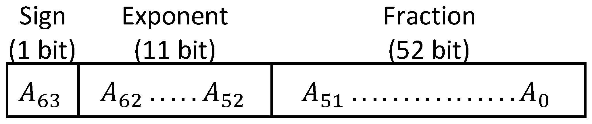
Based on IEEE 754 standard, a 64-bit floating-point number, A, consists of three parts: (1) the sign bit, (2) the exponent, and (3) the fraction, as shown in Figure 1. Starting from left to right, the most significant bit, , represents the sign bit. If is 1, the number is negative; otherwise, it is considered as a positive number. The exponent portion is indicated with the next 11 bits, . Lastly, the 52 least significant bit, , show the mantissae which is a number between 1 and 2 (note that the 1 is implicit and the 52 LSB bits, store a fractional value).
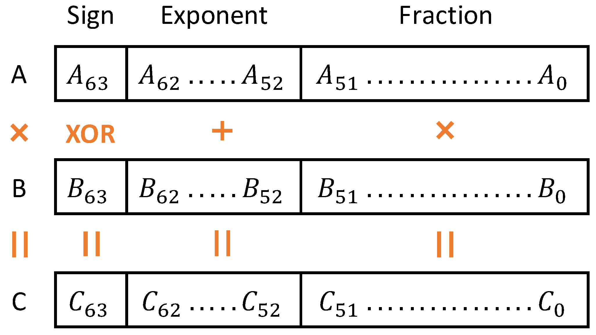
Given two such numbers, A and B, the multiplication can be accomplished through a three-step operation. Based on Figure 2, the sign bit of the result, , is calculated by XORing and . Adding the exponent portions of the inputs leads to the exponential value of the result. And the 52-bit fractional value or mantissa is equal to the product of input fractions.
2.2. Related Work
In this section, we review some of the prior research that focuses on approximate multipliers. Mohapatra et al. [9] propose to design techniques that enable the hardware implementations to scale more gracefully under the presence of voltage over-scaling. Hashemi et al. [5] proposed a dynamic and fast bit selection scheme to reduce the size of multipliers. Vahdat et al. [10] proposed a scalable approximate sequential multiplier which reduces the number of partial products by truncating each of the input operands based on their leading-one bit position. In [7,11], smaller approximate and low-power multipliers are first designed, and then, they are used as basic building blocks to form larger multipliers. References [12,13] proposed to employ approximate adders like iCAC [14] or CMA [12] for calculating the summation of the partial products, or to skip some of the least significant bits. Imani et al. proposed the CFPU, CMUL, and RMAC in [15,16,17], respectively. CFPU and CMUL are configurable floating-point multiplier, and they decide to operate in the approximate or exact mode by examining only one of the input mantissae. RMAC uses addition for manitssae product computation, instead of multiplying them [17]. In [18], Jiao et al. proposed a multiplier which exploits the computation reuse opportunities and enhance them by performing approximate pattern matching.
Due to the inherent resilience of Neural Networks (NNs) to errors, many prior works have proposed to apply approximate computing to DNNs for exploiting power and area efficiency. In [19], Venkataramani et al. proposed the characterization of neurons into resilient and sensitive neurons. Then, the resilient neurons are replaced with their approximate counterparts. Zhang et al. proposed to improve the power consumption and the delay by overlooking uncritical memory accesses [20]. Floating-point multiplication is one of the most key units in DNNs that consume a vast majority of the whole DNNs energy and silicon budget. Therefore, some prior work attempted on reducing the power consumption and area occupation of the DNNs by investigating the benefits of approximate multipliers when employed in a DNN. In [21], Sarwar et al. proposed an approximate multiplier that utilize the notion of computation sharing to achieve improved energy consumption. Neshatpour et al. proposed Iterative CNN by reformulating the CNN from a single feed-forward network to a series of sequentially executed smaller networks and allows the CNN function to be approximated by creating the early termination, with far fewer operations compared to a conventional CNN [22].
3. Proposed Method
3.1. Approximate Mantissa Product Computation: The Comparator-Enabled Multipliers (CEM)
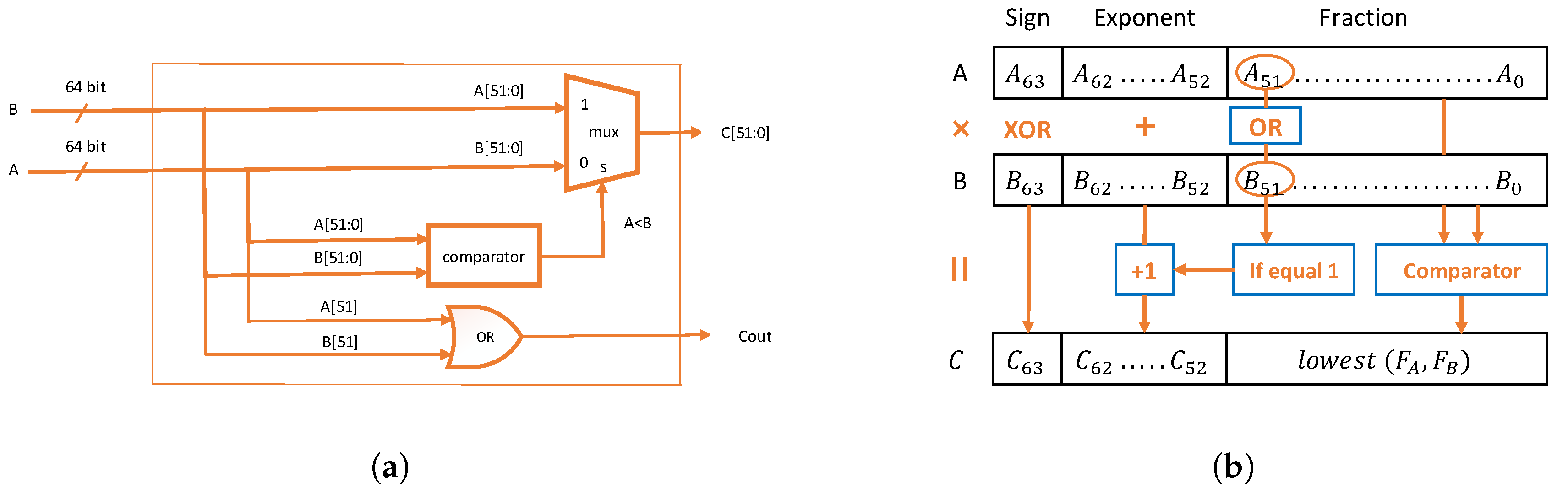
We propose to use a CEM unit instead of an accurate multiplier for the calculation of mantissae product. A CEM unit takes two 52-bit mantissae and as inputs, compares them, and outputs the smaller one as their product . Figure 3a shows the implementation of the proposed CEM (as shown in Figure 3b the is added to the exponent portion of the final result). Employing a CEM as an alternative for an accurate multiplier decreases the power consumption and area of the FP multiplier, significantly. Note that the proposed CEM consumes less power and area than an accurate comparator. Owing to the fact that the CEM only identifies the smaller operand (i.e., it only outputs the signal ). Hence, it does not contain the required logic for identifying and . After a thorough investigation, we realize that the proposed CEM has a relatively lower error under two conditions: (1) when the absolute difference between the operands is rather significant, or (2) at least one of the operands is roughly equal to 2 or 1. Apart from that, the degradation in accuracy is relatively higher. We perform excessive simulations to justify the validity of these two conditions. Since the mantissae is always between 1 and 2, we consider perform our simulations on this range, i.e., .
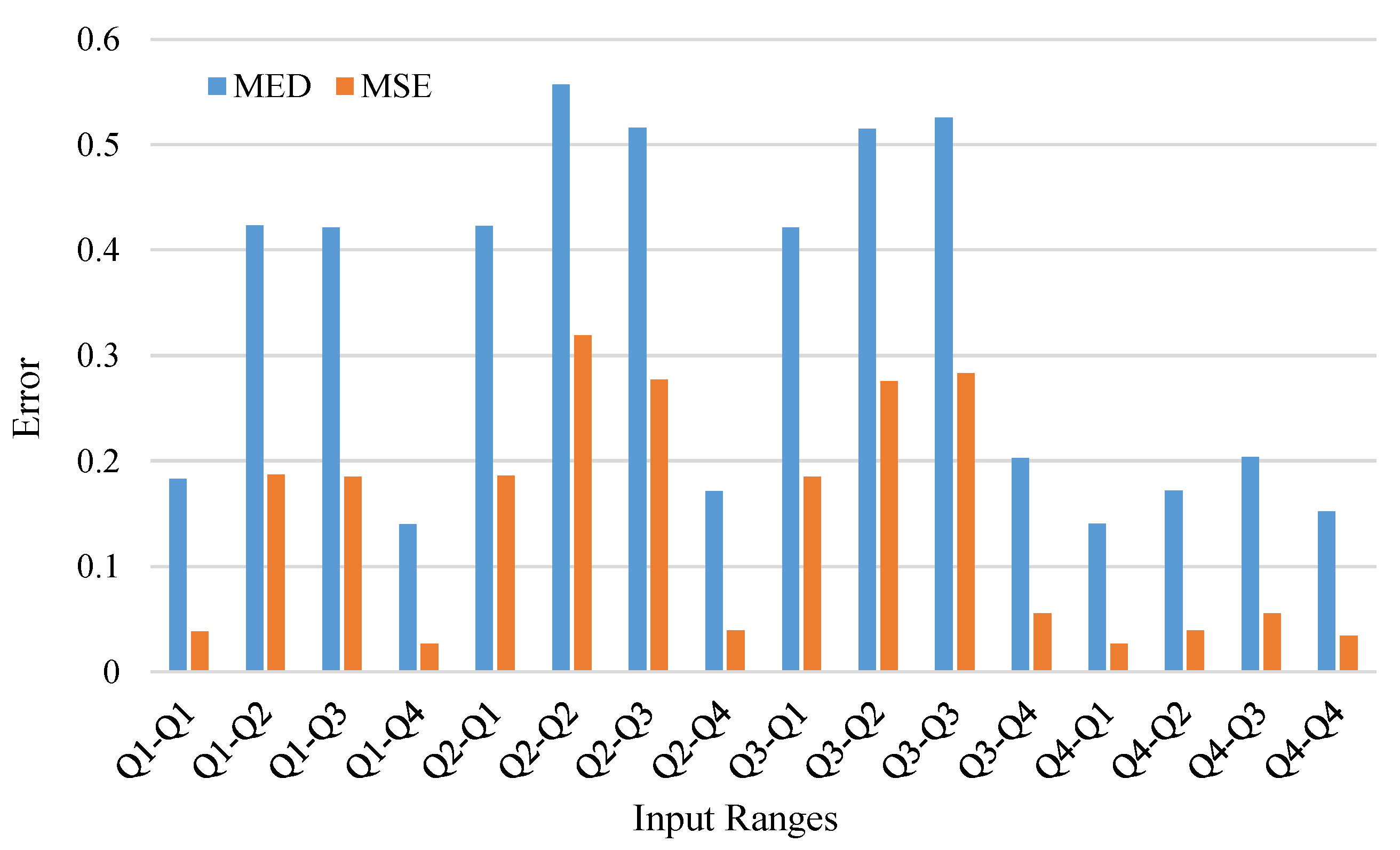
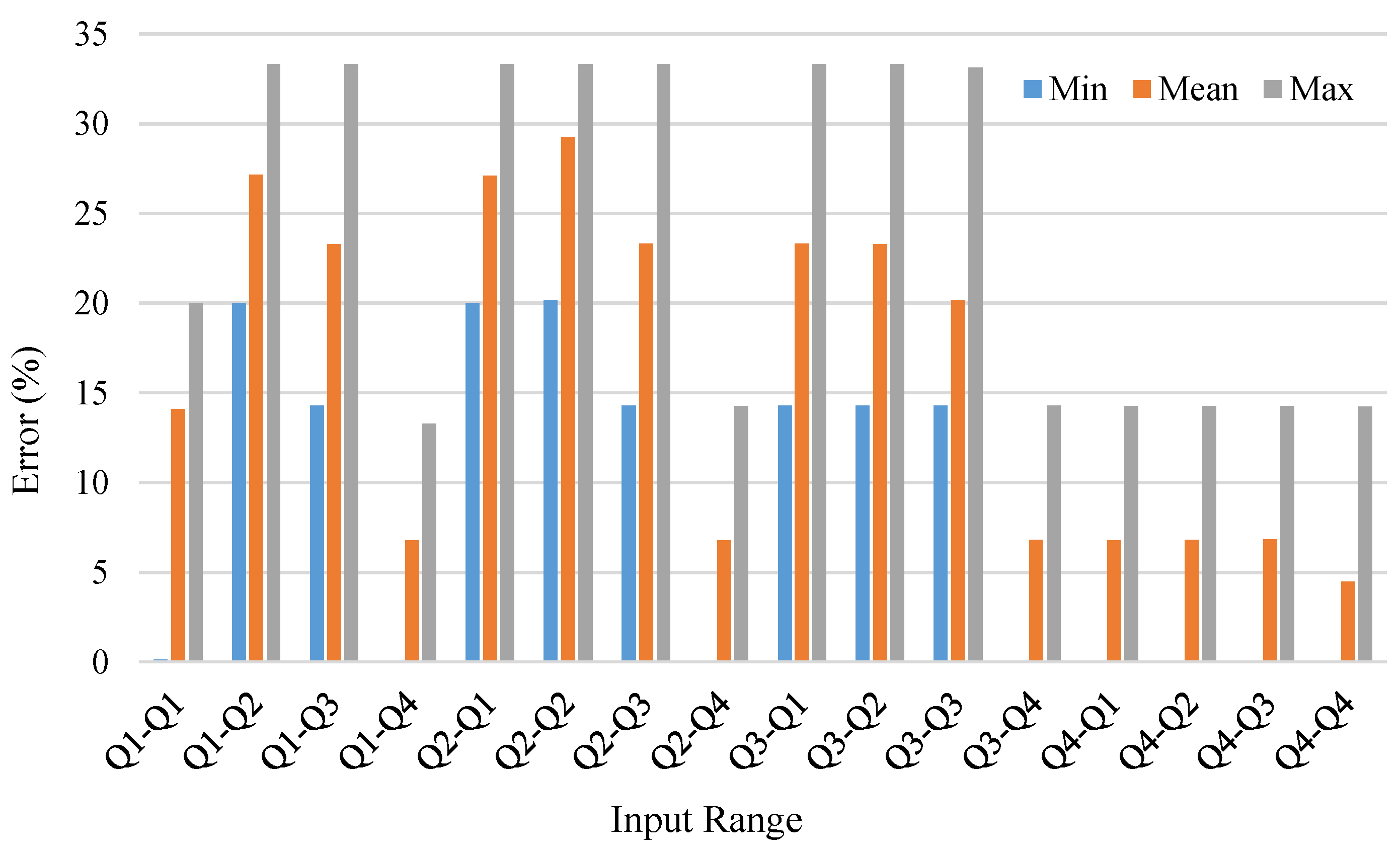
In Figure 4, we divide each of the input mantissae into four quarters (denoted with to ), based on their proximity to 1. Each quarter refers to a specific range for the input mantissae; (1) for the mantissa is in the range , (2) for the mantissa is in the range , (3) for the mantissa is in the range , and (4) for the mantissa is in the range . Each pair of input ranges are identified using the notation , where . For example, refers to a case where the first input is in the range , and the second input is in the range . This leads to 4×4 combinations of input ranges. Figure 4 demonstrates the error of the proposed CEM over each of these 16 input ranges, in terms of MED and MSE metrics. Figure 5 shows the error percentage of the CEM. These metrics are evaluated over 10000 randomly generated numbers—in Figure 4 and Figure 5 all three metrics follow almost the same trend; thus, we only investigate the errors through the MED metric. As shown in Figure 4, for six input ranges, at least one input is close to 2 (i.e., there is at least one , e.g., and ), thus they have relatively smaller MED. Within these six input ranges, as the difference between the two inputs enlarges (or one input gets closer to 1), the error gets smaller. This is why and have the lowest errors. For , both input ranges are close to 1; therefore, it has a relatively small MED. The same error pattern can be seen for other input ranges as well, i.e., as the absolute difference between two numbers enlarges, the error gets reduced. Also, as one input gets closer to 2 or 1, the error decreases.
3.2. AxCEM: Approximate Comparator-Enabled Multipliers
We propose to apply approximate computing to the proposed CEM to further reduce its power consumption, area occupation, and delay. By applying logic simplifications to the CEM, we propose two novel approximate CEMs, namely “AxCEM1” and “AxCEM2”. The main idea for improving the circuit metrics (i.e., the power consumption, silicon area, and the delay) is to simplify the boolean equations of the CEM. However, this simplification is accomplished in a way that it preserves the accuracy at an acceptable range. This, prior to the logic simplification, requires a thorough examination of the CEM error for different input ranges (similar to Figure 4 and Figure 5). Next, the logic responsible for the error at a specific range should be modified in a way that it consumes less power and area, compared to the proposed CEM. Note that such logic simplifications, although improve the circuit metrics, often entail some amount of accuracy loss. However, we show our approach for simplifying the CEM logic, while decreases the accuracy in some cases, may lead to accuracy improvements for other input ranges. For the sake of simplicity, we illustrate our approach on 3 MSB bits of the proposed CEM over input range. We choose because it is one of the input ranges in which the CEM has relatively low accuracy.
Step 1. We examine the error histogram of the CEM for a specific input range. Then, we check if it mostly contains negative or positive errors. If the vast majority of errors are positive, the CEM should be under-approximated, i.e., the approximate results should be less than the accurate results, averagely. Otherwise, the equation should be simplified (approximated) in a way that generates results that are larger than the accurate results (over-approximated).
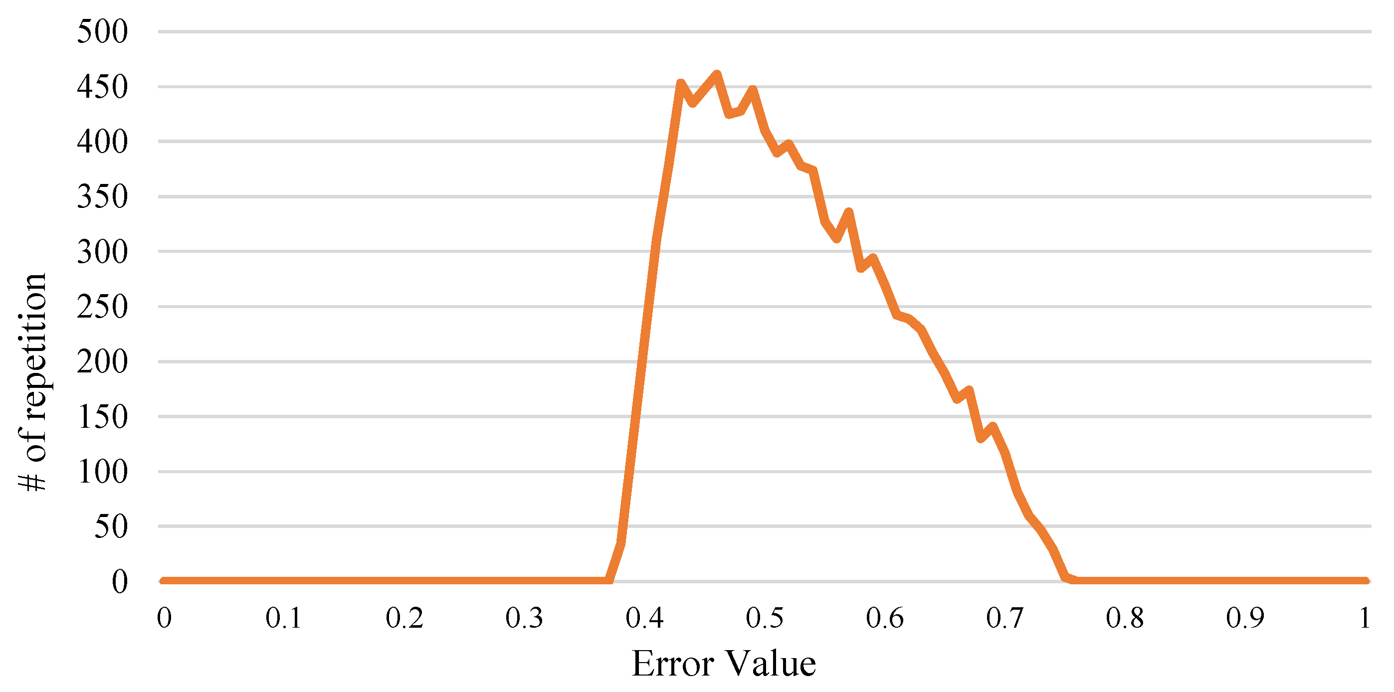
Figure 6 demonstrates the error histogram of the CEM over input range. As shown in Figure 6, all errors are positive, having their values between 0.35 to 0.75. Thus, a logic simplification that under-approximate the CEM may have to cause the lowest accuracy loss—this approach might even lead to accuracy improvements because it cancels some of the positive errors.
Step 2. For the case of under-approximation, the simplifications should result in more 0s in the outputs. Conversely, for over-approximation, we simplify the boolean equations of CEM in a way that the simplified version tends to generate more 1s in the output.
In our example, step 1 concludes that under-approximation sounds a viable approach for logic simplification. Moreover, the errors with the highest number of repetitions are in the range of 0.4 to 0.5. Therefore, if the approximation leads to a -0.5 error in comparison with the CEM, the accuracy loss will be quite low. Bit position 51 has a value of 0.5. Hence, if the CEM results have a 1 in bit position 51, the approximate version should result in a 0 in the same bit position. Equation (1) shows the boolean equations for 3 MSBs of the proposed CEM. In our example, for each bit position, we simplify the CEM equations while satisfying two conditions: (1) the approximation should result in a less complex gate-level circuit, and (2) deduced from step 1 & 2, the simplification must lead to more 0s in the results, on average.
Equations (2) and (3) show two approximations of the proposed CEM, AxCEM1 and AxCEM2. For AxCEM1, the AND gate in the MSB of the CEM is replaced with a NOT gate. There are two reasons for doing so: (1) the power consumption and area is reduced, and (2) in the input range , both and are always 1; therefore, this approximation causes a −0.5 decrease in the final result. Note that employing either one of or has the same impact on both circuit and error metrics. In AxCEM2, the same idea is implemented using a NOR gate. In the CEM structure, the boolean equations for calculating the LSB bits of the output are more complex than those of the MSB bits. Thus, the LSB bits are more suitable for exploiting power, area, and delay improvements through aggressive logic simplifications while the accuracy decrease is kept relatively low. Therefore, for bit positions 50 and 49, reducing the power consumption, area occupation, and the delay has a higher priority than preserving the accuracy. As can be seen in Equations (2) and (3), the number of gates required for bit 49 and 51 are drastically reduced. At the same time, the total delay is reduced because and (in Equations (2) and (3)) does not take any inputs from their higher bit positions.
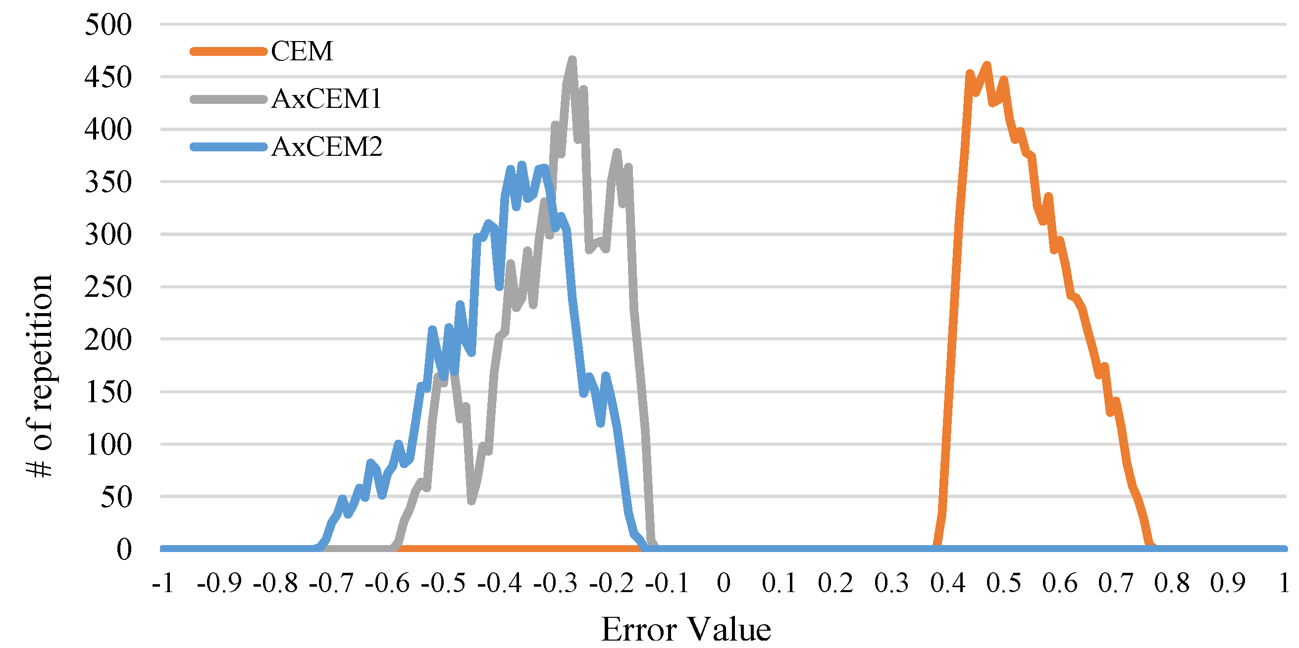
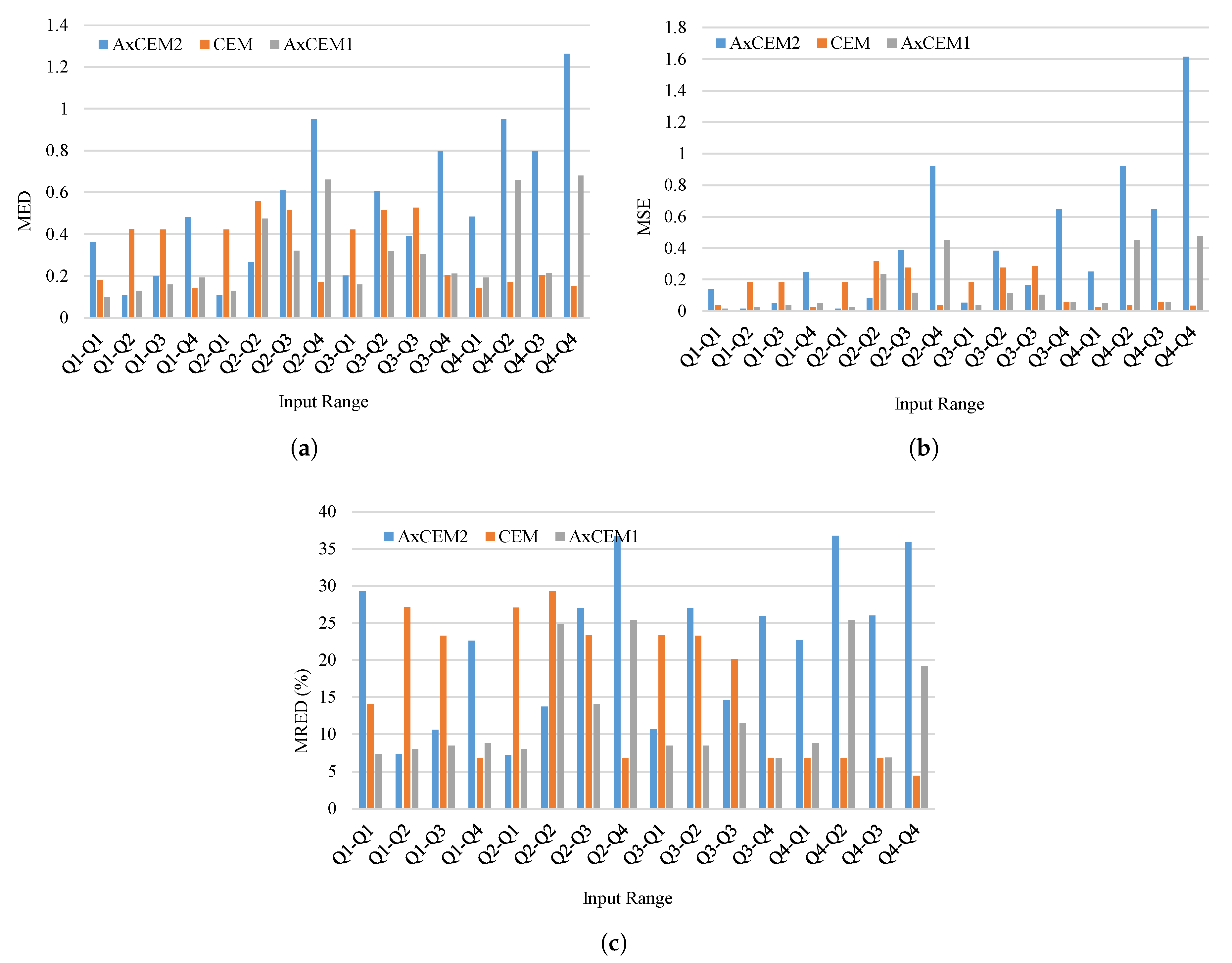
After applying this approach for all 52 bits of mantissae, the error histograms of AxCEM1 and AxCEM2 become as Figure 7. Based on Figure 7, errors of the proposed AxCEM1 and AxCEM2 are all negative. The error of AxCEM1 starts from −0.1 and ends with −0.6, and the most repetition occurs for errors ranging from −0.2 to −0.4. Therefore, AxCEM1 is expected to have less average error (i.e., MED, MSE, and MRED) than the CEM. For AxCEM2, the error range is from −0.1 to −0.7, and the most repeated errors are in range −0.3 to −0.5, which is slightly lower than those of the CEM. Figure 8 shows the MED, MSE, and the MRED for the proposed CEM, AxCEM1, and AxCEM2 for all input ranges. Despite the aggressive approximation performed for AxCEM1 and AxCEM2, Figure 8a–c shows that these two designs have higher accuracy than the CEM over several input ranges. As an example, Figure 8a shows that for input range the MED of AxCEM1 and AxCEM2 are 0.4 and 0.3, respectively, while the MED for CEM is more than 0.5. This is because the approach was mostly oriented on input range . After applying this approach for all 52 bits of mantissae, the error histograms of AxCEM1 and AxCEM2 become as Figure 7. Based on Figure 7, errors of the proposed AxCEM1 and AxCEM2 are all negative. The error of AxCEM1 starts from −0.1 and ends with −0.6, and the most repetition occurs for errors ranging from −0.2 tp −0.4. Therefore, AxCEM1 is expected to have less average error (i.e., MED, MSE, and MRED) than the CEM. For AxCEM2, the error range starts from −0.1 to −0.7, and the most repeated errors are in range −0.3 to −0.5, which is slightly lower than those of the CEM. Figure 8 shows the MED, MSE, and the MRED for the proposed CEM, AxCEM1, and AxCEM2 for all input ranges. Despite the aggressive approximation performed for AxCEM1 and AxCEM2, Figure 8a–c shows that these two designs have higher accuracy than the CEM over several input ranges. As an example, Figure 8a shows that for input range the MED of AxCEM1 and AxCEM2 are 0.4 and 0.3, respectively, while the MED for CEM is more than 0.5. This is because the approach was mostly oriented on input range .
4. Evaluation
This section assesses the performance (i.e., both circuit and error metrics) of the proposed structures. Three state-of-the-art approximate floating-point multipliers, namely, CFPU, RMAC, and CMUL, are chosen as our baselines for comparisons. For circuit metric assessments, we evaluate the static and dynamic power consumption, area occupation, and delay, and we consider them as circuit metrics. To evaluate error metrics, we calculate Mean Error Distance (MED), Mean Squared Error (MSE), and Mean Relative Error Distance (MRED). Moreover, the performance of all designs (i.e., three previous work, three novel designs, and one accurate design) are assessed in two ways; (1) as a standalone structure, and (2) when they are employed in a Convolutional Neural Network (CNN).
4.1. Experiment Setup
For standalone comparisons, all multipliers, both previous and proposed work, are implemented using VHDL description language. The circuit metrics are evaluated using the Synopsys Design Compiler synthesis tool using the NanGate FreePDK45nm library [23]. The Monte Carlo method with 10,000 samples was employed to estimate the MED, MSE, and MRED of multipliers. Based on [2], MED is calculated using Equation (4), and it represents the average of absolute errors over all possible input combinations.
where is the difference between the accurate and approximate result. MSE is represents the average of squared absolute errors for all inputs, as Equation (5) demonstrates [24].
Finally, as shown in 6, MRED refers to the average of relative absolute errors over all applicable inputs [3].
where is the correct result of the input pair.
To evaluate the impact of approximate multipliers (both previous and proposed ones) on the accuracy of CNNs, operating on MNIST and CIFAR-100 datasets, we replaced the exact multipliers of the CNN with approximate versions. Accordingly, seven CNNs are constructed based on seven different multipliers: (1) the exact multiplier, (2) CFPU, (3) CMUL, (4) RMAC, (5) the proposed exact Comparator-Enabled Multiplier (CEM), (6) the proposed AxCEM1, and (7) the proposed AxCEM2. For the sake of readability, in this section, we refer to the different CNNs with the name of their multipliers, e.g., a CNN that employs the AxCEM1 multiplier is named “AxCEM1-CNN”.
4.2. Circuit and Error Metrics
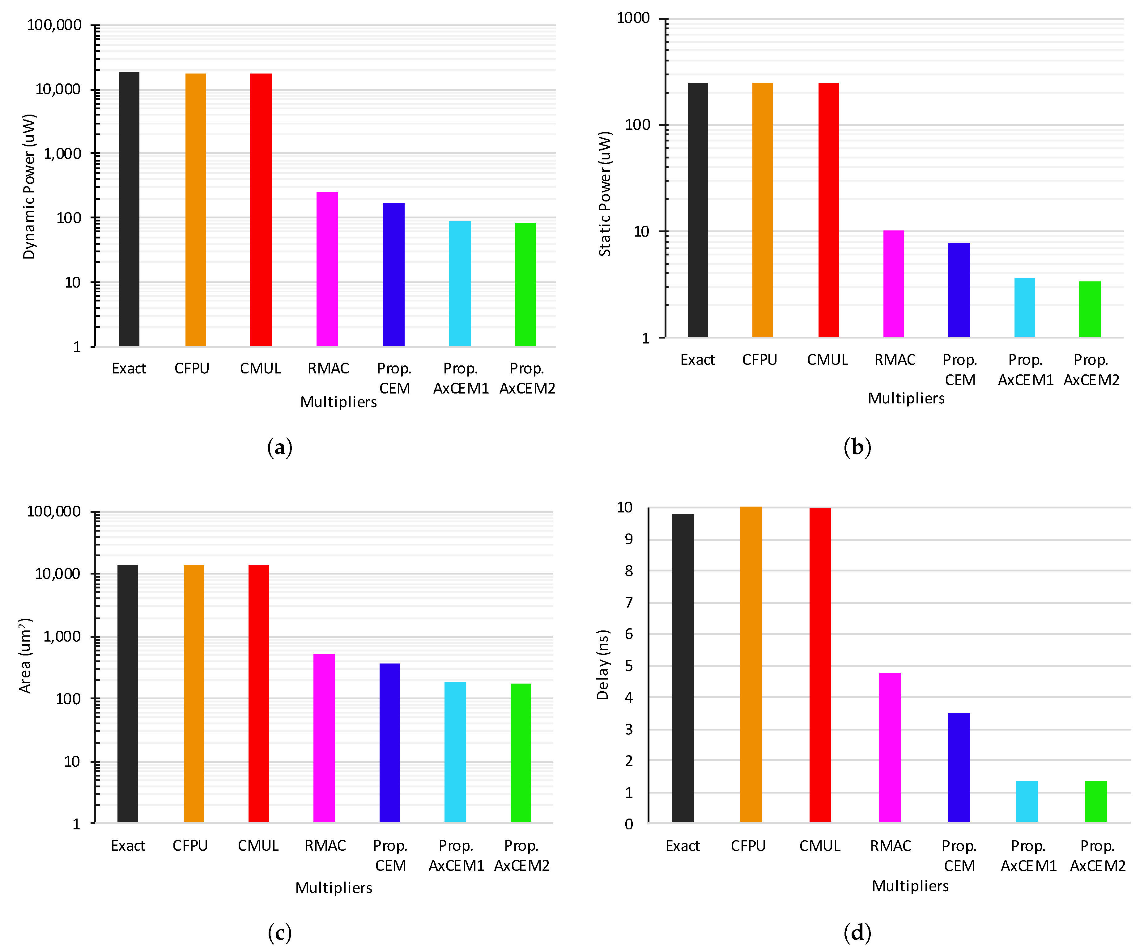
In Figure 9, we compare the circuit metrics (i.e., dynamic and static power consumption, occupied area, and delay) of the proposed designs with those of the exact multiplier and previous approximate ones. Figure 9a,b indicate that regarding the dynamic and static power, all three proposed designs, the CEM, AxCEM1, and AxCEM2 perform the best, followed by RMAC—RMAC also replaces the mantissae product computation unit with a much simpler circuit, i.e., adder. Figure 9a shows that the proposed AxCEMs achieve more than two orders of magnitude improvements concerning the dynamic power consumption, compared with the exact, CFPU, and CMUL multipliers. When compared with RMAC, proposed CEM, AxCEM1, and AxCEM2 exhibit 30, 65, and 66% improvements, respectively. Likewise, the proposed designs consume less static power by more than one order of magnitude in comparison with the exact, CFPU, and CMUL, and up to 66% when compared with RMAC.
Based on Figure 9c, the proposed designs show superiority compared with other multipliers, demonstrating more than one order of magnitude less silicon footprint compared with the exact, CFPU, and CMUL. They also advance more area efficiency than what RMAC offers, ranging from 29 (for CEM) to 65% (for AxCEM2). Moreover, AxCEMs and CEM operate 7X and 2.8X faster than the exact multiplier (CFPU and CMUL are slightly slower). They also outperform RMAC, exhibiting 1.3X to 3.4X faster response.
The benefits achieved on circuit metrics are mainly due to the idea of replacing the mantissae multiplication unit with a much simpler circuit, the comparator, which, in its own terms, serves a twofold purpose: (1) the comparator itself is more circuit-budget friendlier than a multiplier, and (2) it also provides a good starting point for applying hardware-oriented approximation leading to further hardware savings and performance increase. Nevertheless, all such circuit gains appear at the downside of accuracy loss.
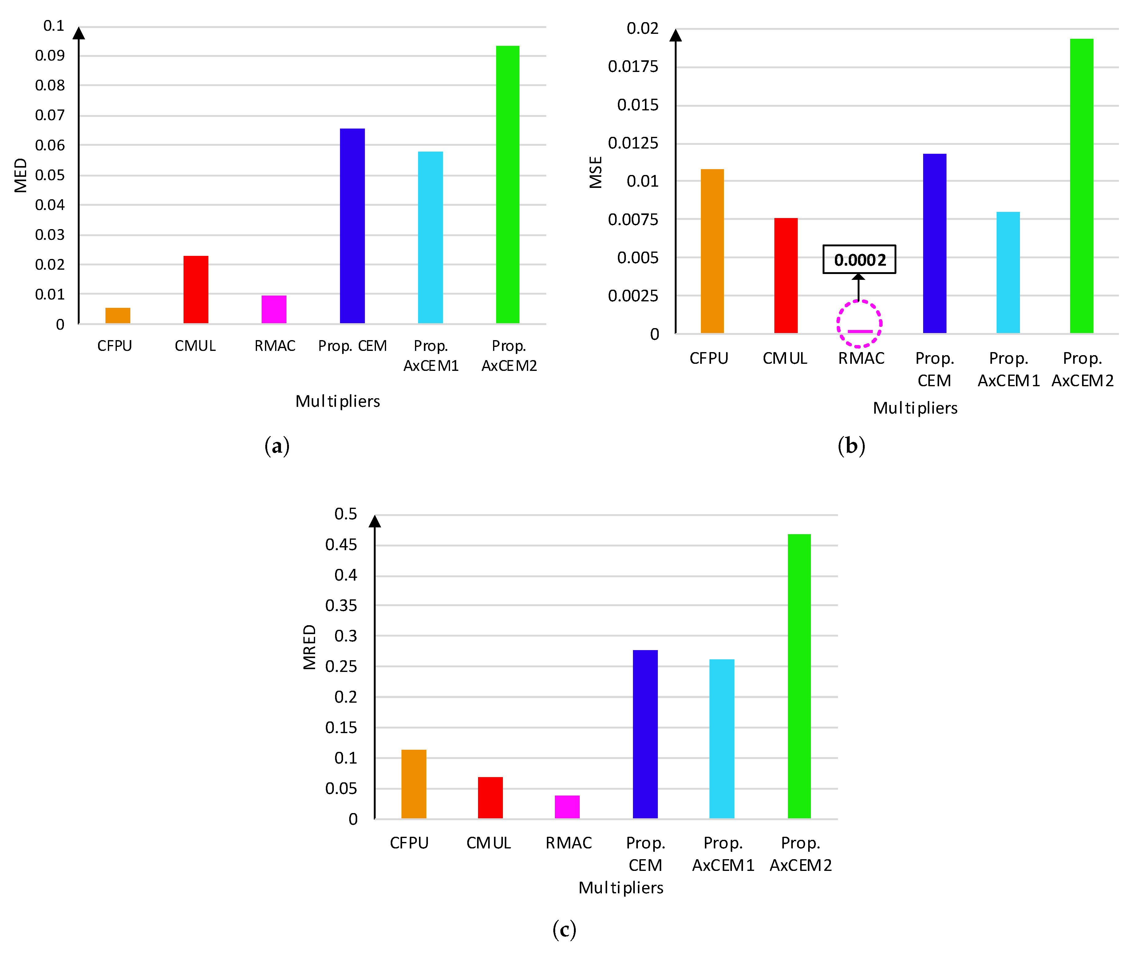
Figure 10 presents error characteristics of the proposed designs in comparison with previous work. Initially, in Figure 4, the MED of CFPU, CMUL, and RMAC are less than 0.03, while the MED of the proposed designs reaches up to 0.1. Regarding MSE in Figure 5, RMAC outperforms other designs, followed by CMUL and AxCEM1, yet all designs have MSEs less than 0.02. Lastly, as shown in Figure 6, again, RMAC is more accurate than other designs.
It can be seen that despite their advantages in hardware resources, the proposed designs have moderate performances w.r.t error metrics. That being said, these metrics, although they sound suitable for standalone comparisons are rather conservative when it comes to evaluating their performance in more complex systems such as CNNs. Thus, they are anticipated to fail to be a good representative of the whole system’s accuracy for two reasons. First and foremost, complex CNN-like systems include many multi-level addition/multiplication operations in the path from the input to the output layer. In multi-level operation, approximate units in different layers may reduce (or even cancel) the prior computational errors. Thus, a proper error analysis of a complex system must consider such error-reducing (or canceling) properties.
Second, approximate computing is extremely data-dependent. However, the metrics displayed in Figure 10 are evaluated over uniformly distributed input patterns. In such cases, a more realistic evaluation must examine approximate units at each layer, only then, calculate the error metrics over their specific input patterns—because inputs of the next layers are under the influence of their previous layer’s outputs, approximate units at different layers may have a completely different input pattern. To mitigate the outcomes of these two problems coupled with standalone metrics, we aim at evaluating the error behavior of approximate designs with a more realistic approach, i.e., employ them in a CNN and calculate the final accuracy of the CNN.
4.3. CNN Performance
The architectures used for the CNNs over the MNIST and CIFAR-100 datasets are as follows. As shown in Table 1, for MNIST: (1) Inputs are black-and-white images. Thus, we allow 784 () input nodes (neurons), (2) A single convolution layer, comprising twenty convolution filters, is contained within the feature extraction network, (3) The ReLU (Rectified Linear Unit) function takes the outputs of the convolution layer as its inputs, (4) The outputs of the ReLU function are passed to the pooling layer in which the average pooling is performed, (5) The classification of the NN comprises a single hidden layer and an output layer. The hidden layer has 100 nodes that use the ReLU as their activation function. There is a total of 10 classes to classify; thus, the output layer is constructed with 10 nodes, (6) We use the Softmax activation function for output nodes. The architecture for CIFAR-100 dataset is roughly similar to that of MNIST but with the following changes shown in Table 2.
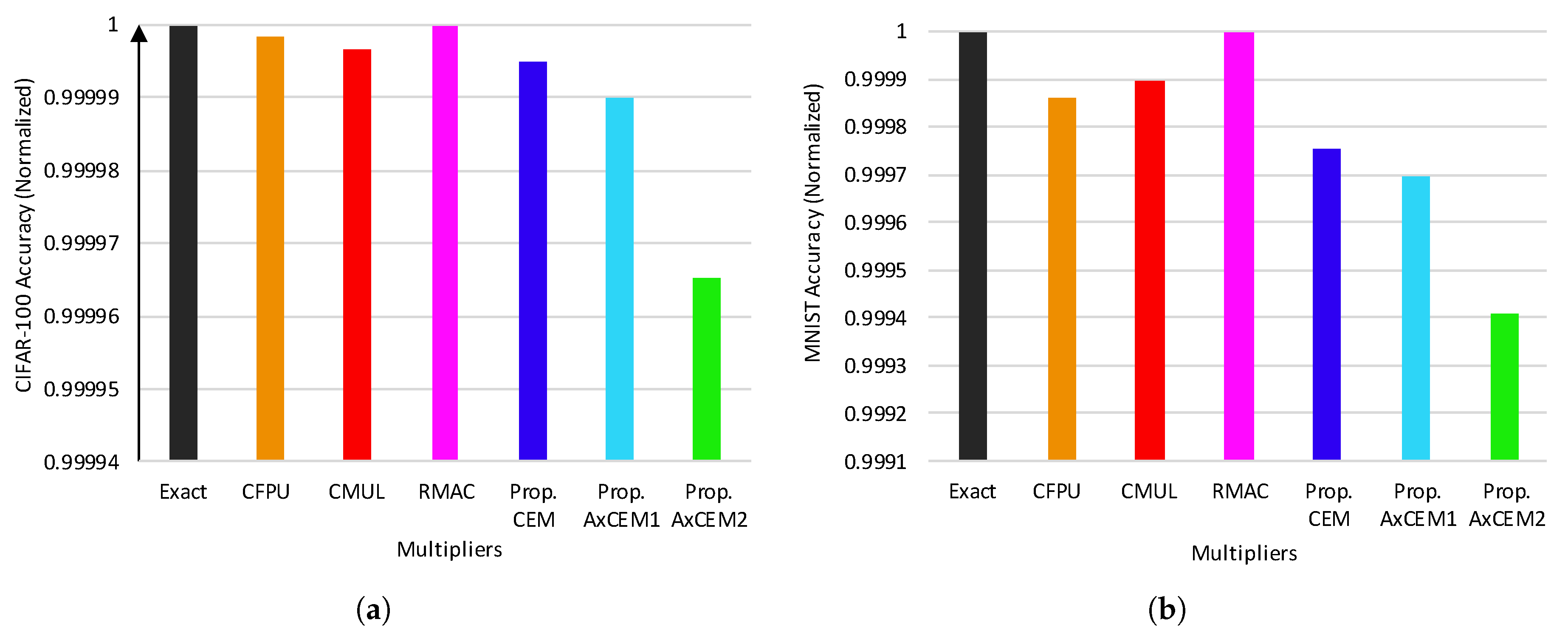
Figure 11 depicts the quality of results of a CNN over two datasets, i.e., CIFAR-100 and MNIST. The vertical axis shows the probability of success for correctly classifying and identifying the input images, and they are normalized based on the exact-CNN. In Figure 11a, it can be seen that the accuracy of CEM-CNN matches to that of exact-CNN up to the fifth decimal place. AxCEM1 and AxCEM2-CNN show small degradations in the accuracy compared to exact, CFPU, CMUL, and RMAC. For the MNIST dataset, the proposed designs-based CNN accuracy loss reaches up to 0.06%—the probability of success for exact-CNN and AxCEM2 is 96.6921% and 96.6348%, respectively.
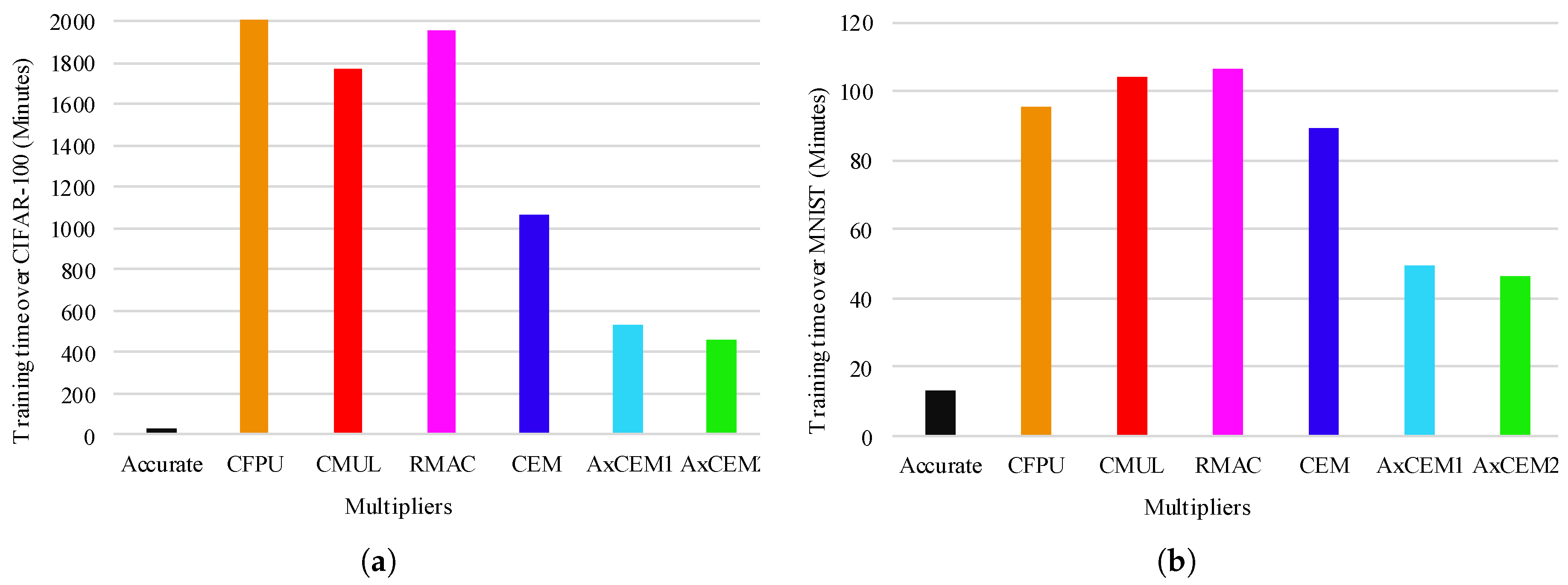
As shown in Figure 12, for the training step, in general, the training time for CNNs employing the approximate multipliers is higher than the accurate-CNN. However, the CNNs employing the proposed designs (i.e., CEM, AxCEM1, and AxCEM2) takes a shorter time to be trained in comparison with the CNNs based on the prior approximate multipliers (i.e., CFPU, CMUL, and RMAC). For CIFAR-100 dataset, Figure 12a shows that the CNNs based on the proposed designs are trained at least 25% faster than the prior wok-based CNNs. Based on Figure 12a, the training times for CFPU-CNN, CMUL-CNN, and RMAC-CNN are more than 1600 minutes, while the proposed CEM-CNN, AxCEM1-CNN, and AxCEM2-CNN, are trained in less than 1200 minutes. For MNIST, the CNNs employing the proposed designs show better performance in comparison with the prior approximate multipliers based CNNs. Figure 12b shows that the CMUL and RMAC-CNNs take more than 100 minutes to train. And the training time for CFPU-CNN is 95 minutes. For the CEM, AxCEM1, and AxCEM2-CNNs the training times are 89, 49 and 45 minutes, respectively. In summary, the results insinuate that although the proposed designs, when considered as standalone designs, perform poorly w.r.t. MED, MSE, and MRED, they are quite good candidates for approximating CNNs as a whole, due to there negligible accuracy loss when employed so.
5. Conclusions
In this paper, floating-point multipliers that can approximately perform the computation with significantly lower energy and higher performance are proposed. Our methodology, employing a Comparator-Enabled Multiplier (CEM), suggests that instead of multiplying fractions, the smaller fraction can be passed as the product output. Subsequently, two approximate versions of CEM, AxCEM1, and AxCEM2, were presented to improve the circuit and error metrics of the CEM. In comparison with other approximate designs, we achieve a 66% reduction in energy consumption. The value of the MRED of the proposed approach Maximum equaled to 47%. The result of MRED indicated more error in calculations, but when used proposed structures in CNN, the value of error achieved a maximum 0.06%. Moreover, the CNNs employing the proposed designs takes a shorter time (at least, 6% over the MNIST and 25% over CIFAR-100 datasets) to be trained in comparison with the CNNs based on the prior approximate multipliers. The results indicate that the train feature of CNN could reduce the influence of the proposed error structures. Therefore, it could be concluded that the MRED, MSE, and MED are not suitable criteria for evaluating the error of computational units. Accordingly, the error of the proposed structure should be evaluated in real applications.
Author Contributions
Conceptualization and methodology is done by S.G., M.D., and M.N.B. Software, validation, formal analysis, and investigation is done by M.R. and S.G. Writing original draft preparation is done by S.G. and M.R. Writing review and editing is done by M.R., M.D. and M.N.B. Visualization, supervision, and project administration is done by M.D. and M.N.B. All authors have read and agreed to the published version of the manuscript.
Funding
This research received no external funding.
Conflicts of Interest
The authors declare no conflict of interest.
References
- Sekanina, L. Introduction to approximate computing: Embedded tutorial. In Proceedings of the 2016 IEEE 19th International Symposium on Design and Diagnostics of Electronic Circuits & Systems (DDECS), Kosice, Slovakia, 20–22 April 2016; IEEE: Piscataway, NJ, USA, 2016; pp. 1–6. [Google Scholar]
- Liang, J.; Han, J.; Lombardi, F. New metrics for the reliability of approximate and probabilistic adders. IEEE Trans. Comput. 2012, 62, 1760–1771. [Google Scholar] [CrossRef]
- Yin, P.; Wang, C.; Liu, W.; Lombardi, F. Design and Performance Evaluation of Approximate Floating-Point Multipliers. In Proceedings of the 2016 IEEE Computer Society Annual Symposium on VLSI (ISVLSI), Pittsburgh, PA, USA, 11–13 July 2016; pp. 296–301. [Google Scholar] [CrossRef]
- Qiqieh, I.; Shafik, R.; Tarawneh, G.; Sokolov, D.; Yakovlev, A. Energy-efficient approximate multiplier design using bit significance-driven logic compression. In Proceedings of the Conference on Design, Automation & Test in Europe, Lausanne, Switzerland, 27–31 March 2017; European Design and Automation Association: Leuven, Belgium; pp. 7–12. [Google Scholar]
- Hashemi, S.; Bahar, R.; Reda, S. DRUM: A dynamic range unbiased multiplier for approximate applications. In Proceedings of the IEEE/ACM International Conference on Computer-Aided Design, Austin, TX, USA, 2–6 November 2015; IEEE Press: Piscataway, NJ, USA, 2015; pp. 418–425. [Google Scholar]
- Rizzo, R.G.; Calimera, A. Implementing Adaptive Voltage Over-Scaling: Algorithmic Noise Tolerance vs. Approximate Error Detection. J. Low Power Electron. Appl. 2019, 9, 17. [Google Scholar] [CrossRef] [Green Version]
- Kulkarni, P.; Gupta, P.; Ercegovac, M. Trading accuracy for power with an underdesigned multiplier architecture. In Proceedings of the 2011 24th Internatioal Conference on VLSI Design, Chennai, India, 2–7 January 2011; IEEE: Piscataway, NJ, USA, 2011; pp. 346–351. [Google Scholar]
- Huang, J.; Lach, J.; Robins, G. A methodology for energy-quality tradeoff using imprecise hardware. In Proceedings of the 49th Annual Design Automation Conference, San Francisco, CA, USA, 3–7 June 2012; ACM: New York, NY, USA, 2012; pp. 504–509. [Google Scholar]
- Mohapatra, D.; Chippa, V.K.; Raghunathan, A.; Roy, K. Design of voltage-scalable meta-functions for approximate computing. In Proceedings of the 2011 Design, Automation Test in Europe, Grenoble, France, 14–18 March 2011; pp. 1–6. [Google Scholar] [CrossRef]
- Vahdat, S.; Kamal, M.; Afzali-Kusha, A.; Pedram, M. TOSAM: An Energy-Efficient Truncation- and Rounding-Based Scalable Approximate Multiplier. IEEE Trans. Very Large Scale Integr. (VLSI) Syst. 2019, 27, 1161–1173. [Google Scholar] [CrossRef]
- Lin, C.; Lin, I. High accuracy approximate multiplier with error correction. In Proceedings of the 2013 IEEE 31st International Conference on Computer Design (ICCD), Asheville, NC, USA, 6–9 October 2013; pp. 33–38. [Google Scholar] [CrossRef]
- Yang, T.; Ukezono, T.; Sato, T. A low-power high-speed accuracy-controllable approximate multiplier design. In Proceedings of the 2018 23rd Asia and South Pacific Design Automation Conference (ASP-DAC), Jeju Island, Korea, 22–25 January 2018; pp. 605–610. [Google Scholar] [CrossRef]
- Baba, H.; Yang, T.; Inoue, M.; Tajima, K.; Ukezono, T.; Sato, T. A Low-Power and Small-Area Multiplier for Accuracy-Scalable Approximate Computing. In Proceedings of the 2018 IEEE Computer Society Annual Symposium on VLSI (ISVLSI), Hong Kong, China, 8–11 July 2018; pp. 569–574. [Google Scholar] [CrossRef]
- Yang, T.; Ukezono, T.; Sato, T. Low-Power and High-Speed Approximate Multiplier Design with a Tree Compressor. In Proceedings of the 2017 IEEE International Conference on Computer Design (ICCD), Boston, MA, USA, 5–8 November 2017; pp. 89–96. [Google Scholar] [CrossRef]
- Imani, M.; Peroni, D.; Rosing, T. CFPU: Configurable floating point multiplier for energy-efficient computing. In Proceedings of the 2017 54th ACM/EDAC/IEEE Design Automation Conference (DAC), Austin, TX, USA, 18–22 June 2017; pp. 1–6. [Google Scholar] [CrossRef] [Green Version]
- Imani, M.; Garcia, R.; Gupta, S.; Rosing, T. Hardware-Software Co-design to Accelerate Neural Network Applications. J. Emerg. Technol. Comput. Syst. 2019, 15, 21:1–21:18. [Google Scholar] [CrossRef]
- Imani, M.; Garcia, R.; Gupta, S.; Rosing, T. RMAC: Runtime Configurable Floating Point Multiplier for Approximate Computing. In Proceedings of the International Symposium on Low Power Electronics and Design, Seattle, WA, USA, 23–25 July 2018; ACM: New York, NY, USA, 2018. ISLPED ’18. pp. 12:1–12:6. [Google Scholar] [CrossRef]
- Jiao, X.; Akhlaghi, V.; Jiang, Y.; Gupta, R.K. Energy-efficient neural networks using approximate computation reuse. In Proceedings of the 2018 Design, Automation Test in Europe Conference Exhibition (DATE), Dresden, Germany, 19–23 March 2018; pp. 1223–1228. [Google Scholar] [CrossRef]
- Venkataramani, S.; Ranjan, A.; Roy, K.; Raghunathan, A. AxNN: Energy-efficient neuromorphic systems using approximate computing. In Proceedings of the 2014 IEEE/ACM International Symposium on Low Power Electronics and Design (ISLPED), La Jolla, CA, USA, 11–13 August 2014; pp. 27–32. [Google Scholar] [CrossRef]
- Zhang, Q.; Wang, T.; Tian, Y.; Yuan, F.; Xu, Q. ApproxANN: An approximate computing framework for artificial neural network. In Proceedings of the 2015 Design, Automation Test in Europe Conference Exhibition (DATE), Grenoble, France, 9–13 March 2015; pp. 701–706. [Google Scholar]
- Sarwar, S.S.; Venkataramani, S.; Raghunathan, A.; Roy, K. Multiplier-less Artificial Neurons exploiting error resiliency for energy-efficient neural computing. In Proceedings of the 2016 Design, Automation Test in Europe Conference Exhibition (DATE), Dresden, Germany, 14–18 March 2016; pp. 145–150. [Google Scholar]
- Neshatpour, K.; Behnia, F.; Homayoun, H.; Sasan, A. ICNN: An iterative implementation of convolutional neural networks to enable energy and computational complexity aware dynamic approximation. In Proceedings of the 2018 Design, Automation Test in Europe Conference Exhibition (DATE), Dresden, Germany, 19–23 March 2018; pp. 551–556. [Google Scholar] [CrossRef]
- NanGate, Inc. NanGate FreePDK45 Open Cell Library; NanGate, Inc.: Santa Clara, CA, USA, 2008. [Google Scholar]
- Ye, R.; Wang, T.; Yuan, F.; Kumar, R.; Xu, Q. On reconfiguration-oriented approximate adder design and its application. In Proceedings of the 2013 IEEE/ACM International Conference on Computer-Aided Design (ICCAD), San Jose, CA, USA, 18–21 November 2013; pp. 48–54. [Google Scholar] [CrossRef]
Figure 1.
A 64-bit floating point number in IEEE 754 standard.

Figure 2.
The multiplication operation of two 64-bit floating-point numbers using IEEE 754 standard.
Figure 2.
The multiplication operation of two 64-bit floating-point numbers using IEEE 754 standard.

Figure 3.
The proposed CEM; (a) the proposed CEM mantissae multiplication, (b) the whole floating-point multiplier using the proposed CEM.
Figure 3.
The proposed CEM; (a) the proposed CEM mantissae multiplication, (b) the whole floating-point multiplier using the proposed CEM.

Figure 4.
The MED and MSE of the proposed CEM for different input ranges.

Figure 5.
The error percentage of the proposed CEM for different input ranges.

Figure 6.
The error histogram of the CEM.

Figure 7.
The error histogram of the CEM, AxCEM1, and AxCEM2.

Figure 8.
Error comparison between CEM, AxCEM1, and AxCEM2; (a) MED, (b) MSE, and (c) MRED.

Figure 9.
Standalone comparison of circuit metrics: (a) dynamic power, (b) static power, (c) area, (d) delay.
Figure 9.
Standalone comparison of circuit metrics: (a) dynamic power, (b) static power, (c) area, (d) delay.

Figure 10.
Standalone comparison of error metrics: (a) MED, (b) MSE, (c) MRED.

Figure 11.
Accuracy comparison of the CNN provided with two different datasets: (a) CIFAR-100, (b) MNIST.
Figure 11.
Accuracy comparison of the CNN provided with two different datasets: (a) CIFAR-100, (b) MNIST.

Figure 12.
The comparison between training times of the CNNs over the two different datasets: (a) CIFAR-100, (b) MNIST.
Figure 12.
The comparison between training times of the CNNs over the two different datasets: (a) CIFAR-100, (b) MNIST.


Table 1.
The CNN architecture over MNIST dataset.
| Layer | Remark | Activation Function |
|---|---|---|
| Input | nodes | – |
| Convolution | 20 convolution filters () | ReLU |
| Pooling | Mean Pooling () | – |
| Hidden | 100 nodes | ReLU |
| Output | 10 nodes | Softmax |
Table 2.
The CNN architecture over CIFAR-100 dataset.
| Layer | Remark | Activation Function |
|---|---|---|
| Input | nodes | – |
| Convolution | 128 convolution filters () | ReLU |
| Pooling | Mean Pooling () | – |
| Hidden | 256 nodes | ReLU |
| Output | 100 nodes | Softmax |
© 2020 by the authors. Licensee MDPI, Basel, Switzerland. This article is an open access article distributed under the terms and conditions of the Creative Commons Attribution (CC BY) license (http://creativecommons.org/licenses/by/4.0/).
Share and Cite
MDPI and ACS Style
Ghabraei, S.; Rezaalipour, M.; Dehyadegari, M.; Nazm Bojnordi, M. AxCEM: Designing Approximate Comparator-Enabled Multipliers. J. Low Power Electron. Appl. 2020, 10, 9. https://0-doi-org.brum.beds.ac.uk/10.3390/jlpea10010009
AMA Style
Ghabraei S, Rezaalipour M, Dehyadegari M, Nazm Bojnordi M. AxCEM: Designing Approximate Comparator-Enabled Multipliers. Journal of Low Power Electronics and Applications. 2020; 10(1):9. https://0-doi-org.brum.beds.ac.uk/10.3390/jlpea10010009
Chicago/Turabian StyleGhabraei, Samar, Morteza Rezaalipour, Masoud Dehyadegari, and Mahdi Nazm Bojnordi. 2020. "AxCEM: Designing Approximate Comparator-Enabled Multipliers" Journal of Low Power Electronics and Applications 10, no. 1: 9. https://0-doi-org.brum.beds.ac.uk/10.3390/jlpea10010009
Note that from the first issue of 2016, this journal uses article numbers instead of page numbers. See further details here.