
Analog Filters Design for Improving Precision in Proton Sound Detectors


1
Department of Physics, University of Milano-Bicocca, 20126 Milan, Italy
2
INFN Section of Milano-Bicocca, 20126 Milan, Italy
*
Author to whom correspondence should be addressed.
J. Low Power Electron. Appl. 2021, 11(1), 12; https://0-doi-org.brum.beds.ac.uk/10.3390/jlpea11010012
Submission received: 4 February 2021
/
Revised: 14 March 2021
/
Accepted: 16 March 2021
/
Published: 18 March 2021
Abstract
:This paper analyzes how to improve the precision of ionoacoustic proton range verification by optimizing the analog signal processing stages with particular emphasis on analog filters. The ionoacoustic technique allows one to spatially detect the proton beam penetration depth/range in a water absorber, with interesting possible applications in real-time beam monitoring during hadron therapy treatments. The state of the art uses nonoptimized detectors that have low signal quality and thus require a higher total dose, which is not compatible with clinical applications. For these reasons, a comprehensive analysis of acoustic signal bandwidth, signal-to-noise-ratio and noise power/bandwidth will be presented. The correlation between these signal-quality parameters with maximum achievable proton range measurement precision will be discussed. In particular, the use of an optimized analog filter allows one to decrease the dose required to achieve a given precision by as much as 98.4% compared to a nonoptimized filter approach.
1. Introduction
Ionoacoustic range verification is a promising method to experimentally measure the range of a proton beam in an absorber. The rapid deposition of energy that occurs at the end of the particle range, in a region called the Bragg peak (BP), generates an acoustic signal that can be acquired by dedicated sensors and used to locate the BP by measuring the time of flight of the acoustic wave. This has many promising applications in the field of oncological hadron therapy, where it promises a real-time and more precise localization than the currently used nuclear imaging techniques (e.g., PET, prompt gamma ray imaging) [1,2,3,4]. Improving the precision in the localization of the BP allows one to monitor the treatment in real time, verifying that the radiation dose is actually administered in the volume to be treated. The ionoacoustic technique was first proposed by Sulak in 1979, while in 1995, Hayakawa observed the first ionoacoustic signal within a patient [5,6]. Numerous experiments have recently been carried out both at preclinical (<65 MeV) and clinical (between 65 and 250 MeV) energies [7,8,9,10,11,12,13]. The precision in the localization of the BP is of a few tens of micrometers in preclinical scenarios and in the order of a millimeter at clinical energies. However, the biggest obstacle to the application of this technique in clinical scenarios is the high dose required to obtain these precisions, which are not compatible with clinical treatments. In fact, in clinical scenarios, the acoustic signal is extremely weak (in the milliPascal range). The state of the art uses nonoptimized and general-purpose electronics which limits the achievable signal-to-noise ratio and therefore forces the use of postprocessing (averaging acoustic signals from multiple beam shots) which drastically increases the deposited dose.
For this reason, this paper analyzes the main aspects that make clinical scenarios critical and shows how an optimized analog filter can strongly decrease the dose necessary to obtain a certain precision (defined as the standard deviation of the measured BP position), moving in the direction of a clinical application of the ionoacoustic technique. This paper is organized as follows: Section 2 presents the characteristics of the preclinical and clinical scenarios present in the literature, with a particular focus on the instrumentation used and the signal-to-noise ratio achieved. Section 3 presents a cross-domain model of ionoacoustic experiments and evaluates the main factors that influence measurement precision. Section 4 shows how an optimized analog filter allows one to greatly reduce the dose. Finally, in Section 5, conclusions will be drawn.
2. Ionoacoustic Experimental Setup and Scenarios
Ionoacoustic experimental setups are typically composed of a pulsed particle beam hitting a water phantom where the pressure signal is generated. Then, the pressure signal propagates in water and is sensed by a specific acoustic sensor (AS). The signal transduced into the voltage domain is then conditioned by an analog front end (AFE) and converted in the digital domain where the BP is localized with respect to the AS by measuring the acoustic wave time of flight (ToF). The scheme of a typical ionoacoustic experimental setup is illustrated in Figure 1.
Figure 2 shows how the Bragg curve varies at different beam energies. While at sub-clinical energies the range is a few millimeters, in clinical energies it varies from a few centimeters to a few tens of centimeters to reach tumors located at different depths within the human body. As the range increases, the Bragg peak full width at half-maximum (BPFWHM) and thus the volume of the Bragg peak increases accordingly. This volume does not grow linearly with energy. As a consequence, at high beam energies the energy deposited per unit of mass (called dose, D) becomes lower. Since the amplitude of the pressure signal is proportional to the dose, this means that while at preclinical energies the pressure signal at the BP is of tens or hundreds of Pascals, this value drops to a few Pa or fractions of Pa in clinical scenarios, as shown in the bottom of Figure 2.
Considering the spherical propagation from the BP to the sensor, in preclinical scenarios the sensor acquires signals of a few Pa, while in clinical scenarios this value drops to a few milliPascals. To acquire such weak signals, the state of the art improves the signal-to-noise ratio (SNR) by heavily relying on postprocessing algorithms such as averaging multiple beam shots. However, this increase in SNR comes at the cost of an extra dose. In particular, the SNR and the dose increase with averaging as in Equations (1) and (2), where SNR1sh and SNRavg are the single shot, Nsh is the number of averaged beam shots and the total dose Dtot is Nsh times the single-shot dose D1sh.
Another effect of increasing the BP volume is the decrease in the frequency of the acoustic signal. In particular, while a 20 MeV beam generates a signal whose main frequency is 2 MHz, this value drops to a few tens of kHz at clinical energies. Equation (3) shows the relationship between the signal frequency (fsignal), the sound speed in water cW (~1500 m/s at 30 °C) and the Bragg peak full width at half-maximum (BPFWHM).
This frequency dependance on proton beam energy is shown in Figure 2 (bottom). The next section will show how optimized ionoacoustic detectors reduce extra doses with the same precision, highlighting how an advancement in ionoacoustic detector technology has the potential to bring this technique closer to clinical applications.
3. Factors Influencing Ionoacoustic Measurement Precision
In literature, the precision achieved by a detector is usually evaluated a posteriori by repeating the experimental measurements many times and observing the variance of the data collected. This approach is good for evaluating the achieved performance but does not investigate what factors influence the precision of the result. Without precise information on the relationship between signal characteristics and precision, it is not possible to design a detector knowing in advance that it will achieve a certain desired precision. For this reason, this section investigates the relationship between the main characteristics of the signal and the precision achieved. Noise is added to a typical ionoacoustic signal (bipolar pulse). Noise has a given limited bandwidth and a given SNR.
The ToF is then calculated with different noise realizations, and by evaluating the ToF variance, the measurement precision is estimated as shown in Figure 3. Then, the effect of three different parameters on measurement precision is evaluated. In particular, the three relevant parameters are signal frequency, SNR and noise shaping, defined as the ratio between the signal bandwidth and the noise bandwidth.
3.1. Signal Frequency
Figure 4 shows the dependence of measurement precision on signal frequency for three fixed SNR values. It is possible to see how by decreasing the signal frequency the precision decreases proportionally to 1/f. This relationship is not unexpected when one considers the well-known relationship between resolution and wavelength in acoustic and optical systems. However, in ionoacoustic experiments, this effect explains the difference in performance obtained in the preclinical and clinical experiments. In particular, with the same SNR, switching from a beam at 20 MeV (acoustic signal at 2 MHz) to a beam at 200 MeV (acoustic signal at 40 kHz) implies a reduction in precision by a factor of 50. If in fact 10 dB of SNR results in a precision of about 10 microns at 20 MeV, the same SNR at 200 MeV will correspond to a precision of just 1.5 mm. Similarly, to obtain a precision of 100 microns, 15 dB of SNR will be enough for a 50 MeV beam (600 kHz), while to obtain the same precision with a 150 MeV beam (70 kHz), 30 dB of SNR is required. Clinical scenarios are therefore critical not only for the weakness of acoustic signals, but also for the low frequency of the acoustic signal which intrinsically penalizes the precision of the measurement.
3.2. Signal-to-Noise Ratio
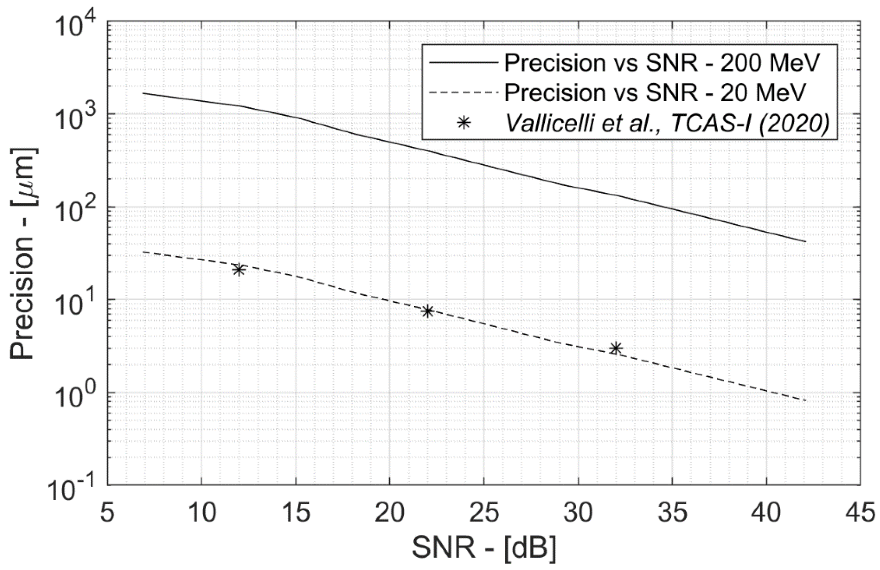
Figure 5 shows the relationship between precision and SNR for the two cases under review, 20 and 200 MeV. It is intuitive to think that at a high SNR, the achievable precision is greater, but having an analytical tool to quantify this ratio is essential to extract the SNR specifications to design a detector that achieves the desired precision. According to Figure 4, the precision at 20 MeV is higher than that at 200 MeV due to the different frequency of the signal.
To validate the results of the model proposed here, the precision results reported in [13] have been inserted. In fact, this paper reports the precision results of an experiment at 20 MeV proton energy together with an accurate characterization of the SNR. It can be seen that the hereby presented model fits perfectly with the experimental data.
Finally, the linear trend in log-log scale shows how the precision is proportional to 1/SNRdB.
3.3. Relative Noise Bandwidth
In addition to the signal frequency and SNR, there is a final factor that has an important impact on precision, and that is the frequency shaping of the noise. In fact, the use of a low-pass filter attenuates the high frequency noise components. This has a double effect. First, it improves the SNR, reducing the noise power. Secondly, reducing the high-frequency components of the noise increases the correlation between adjacent samples. In fact, while white noise (i.e., with a flat power spectral density over a bandwidth much greater than the signal bandwidth) is perfectly uncorrelated, applying a low-pass filtering eliminates the high-frequency components and makes the noise correlated.
To separate the effect of the SNR and noise frequency shaping, we introduce the relative noise bandwidth (RNBW), defined as the ratio between the noise bandwidth BWnoise and the signal frequency.
For high RNBW values, the noise band is much higher than that of the signal (white noise, uncorrelated) while for RNBW values tending to 1 the noise band is always more similar to that of the signal (pink noise, correlated) as shown in Figure 6. For the sake of simplicity, a second-order Butterworth low-pass filter was used, but a more accurate study can be done by varying the type and order of the filter. Figure 7 shows the effect of different RNBW values in a 20 MeV scenario. Given a signal bandwidth of 2 MHz, the RNBW values vary from 100 (200 MHz noise bandwidth, white uncorrelated noise) to 1 (same noise and signal bandwidth). It is interesting to note that the noise bandwidth has a strong impact on precision. For example, considering an SNR of 20 dB, the precision is equal to 32 microns in the case of white noise (RNBW = 100) and improves up to 6 microns in the case of RNBW = 1. This effect can be explained by considering that in white noise, subsequent samples are strongly unrelated. We call xM the sample corresponding to the true maximum point (i.e., evaluated in the absence of noise). In the case of white noise, the adjacent samples are uncorrelated, so it is easy for the samples adjacent to xM to have a very different value to that of xM (variation between a subsequent sample statistically equal to 1 sigma) and can therefore overtake it by moving the position of the point of maximum measured.
Conversely, in the case of correlated noise (low frequency noise), the adjacent samples will have a similar value (variation between one sample and the next, statistically less than 1 sigma), and the variation will be on a larger time scale. It is therefore easier to detect the true maximum point, improving the precision with the same SNR. This effect highlights the importance of proper analog filter sizing, which improves precision by both rejecting high frequency noise (improving SNR) and correlating noise, thus further improving precision. Again, the model results are in good agreement with [14], where a third-order Butterworth with RNBW = 2.5 was used.
3.4. Ionoacoustic Relative Precision
Figure 8 includes and summarizes all the effects shown in the previous sections and can be used as a chart to evaluate the performance of a detector in any scenario. In fact, the precision relative to the dimension of the Bragg peak (BPFWHM) instead of the absolute one is reported on the y-axis. As explained in Section 2, the BPFWHM is equal to half the wavelength of the acoustic signal. Therefore, by plotting relative precision, we automatically include the effect of the signal frequency shown in Figure 4. Thus, Figure 8 is a useful tool to predict the measurement precision in any scenario. In particular, Figure 8 allows one to derive the project specifications for any experimental scenario. For example, to achieve 0.5 mm accuracy with a 200 MeV beam (2.5% wrt BPFWHM) and a 10 mPa0-peak signal at the sensor, Figure 8 shows that 17 dB of SNR will be required with ENBW = 1. This means that the acoustic sensor must have an equivalent noise 17 dB lower than 10 mPa0-peak, that is 1 mPaRMS. In this way, it is possible to obtain the main design specifications for the acoustic sensor (resonance frequency and noise floor) and for the front end (noise figure, filter cutoff frequency, A/D converter characteristics) so that the detector achieves the desired precision.
4. Analog Filter Design for 200 MeV Proton Sound Detector
The results in Section 3 show that the analog filter is a fundamental stage to improve the precision of ionoacoustic detectors. In fact, it allows one to increase the SNR by rejecting out-of-band noise and interference, increasing the precision as shown in Figure 5. It also attenuates the high-frequency noise components, which have a particular impact on precision, as shown in Section 3.3. This section will apply the results of the previous section to show how a dedicated analog filter can improve the performance of ionoacoustic detectors.
The worst-case scenario has been considered and corresponds to the 200 MeV proton beam, as the low frequency and amplitude of the signal make it more difficult to achieve high precisions. This scenario is well characterized in the literature and the typical characteristics are reported in Table 1 [7,10]. This section shows the design of a second-order, fully differential Rauch low-pass filter optimized for this experimental scenario that achieves RNBW = 1. The Rauch filter implements a couple of complex-conjugate poles at a given frequency f0 = 2πω0 and quality factor Q:
The filter scheme is shown in Figure 9.
The −3 dB frequency (13 kHz), Q factor (0.707, corresponding to a Butterworth filter) and gain (G = 1) allow one to dimension the passive components as in (6)–(9) [15]. The main filter parameters and component values are reported in Table 2.
where
Equation (5) allows one to dimension the noise sources (operational amplifier and resistors) so that they are negligible with respect to the noise of the sensor and of the LNA. Figure 10 shows the simulated low-pass filter frequency response.
5. Results—Analog Filter Design Dose Reduction at 200 MeV
In state-of-the-art experiments, little attention is paid to filtering, which usually has cut-off frequencies equal to 10 times the signal or more (RNBW > 10). Figure 11 shows the effect of the optimal filter (RNBW = 1) presented in the previous section and allows one to calculate the reduction in dose with respect to the state of the art. The effects of the dedicated filter are as follows:
- ▪
- The band on which the noise is integrated is limited by a factor of 10, resulting in a 10 dB lower noise power and consequently an SNR increase by the same amount (top of Figure 11).
- ▪
- The reduction of the RNBW allows one to obtain the same precision (for example, of 0.5 mm in the bottom of Figure 11) with an 8 dB lower SNR.
Considering the two combined effects, the use of an optimized filter results in an equivalent 18 dB SNR increase compared to nondedicated state-of-the-art detectors.
This 18 dB increase in SNR is particularly relevant if we consider the extra dose required in the state of the art to achieve the performance of an optimized filter. In fact, the strategy used by the state of the art to improve SNR is based on the average of several successive shots of the beam. However, averaging is inefficient as the noise power decreases with the square root of the number of shots, while the extra dose grows linearly with the number of shots. For this reason, to match the dedicated filter 18 dB SNR increase, the state of the art requires one to shoot the beam 63 times, thus leading to a deposited dose 63 times higher. Comparing these performances with those obtained from the state of the art, [7,10] report a precision of 0.34 mm and 2.2 mm with a dose of 10 Gy and 2 Gy, respectively. Using a dedicated analog filter, it is possible to significantly reduce the dose to just 1.6% (1/63), achieving the same precision with just 160 mGy and 32 mGy, respectively. This promising result shows that the ionoacoustic technique has the potential to be applied in clinical scenarios but highlights that a new generation of dedicated ionoacoustic detectors is needed.
6. Conclusions
This article shows the main aspects that influence precision in a proton range measurement using the ionoacoustic technique. In particular, the signal frequency, SNR and noise bandwidth have a strong impact that must be taken into account when designing a new generation acoustic detector. In fact, most of the experiments present in the state of the art had the objective of characterizing the physical phenomenon, using general-purpose electronics not optimized to the characteristics of the signal itself. This involves an intensive use of postprocessing to improve signal quality in the digital domain, at the cost of a high extra dose not compatible with clinical applications. This paper shows that, by optimizing the detector and in particular the analog filter, it is possible to drastically decrease the dose, bringing this technique closer to clinical applications. The next generation of ionoacoustic detectors will therefore have to focus on optimized and compact instrumentation, which is possible thanks to the use of Application Specific Integrated Circuits (ASICs) [14,15].
Author Contributions
Conceptualization, E.A.V.; writing—original draft preparation, E.A.V.; supervision, M.D.M. All authors have read and agreed to the published version of the manuscript.
Funding
This research was supported by the Proton Sound Detector Project funded by the Italian Institute for Nuclear Physics (INFN).
Conflicts of Interest
The authors declare no conflict of interest.
References
- Knoll, G.F. Radiation Sources. In Radiation Detection and Measurement; John Wiley & Sons: Hoboken, NJ, USA, 2000; pp. 1–28. [Google Scholar]
- Parodi, K.; Polf, J.C. In vivo range verification in particle therapy. Med. Phys. 2018, 45, e1036–e1050. [Google Scholar] [CrossRef] [PubMed] [Green Version]
- Min, C.-H.; Kim, C.H.; Youn, M.-Y.; Kim, J.-W. Prompt gamma measurements for locating the dose falloff region in the proton therapy. Appl. Phys. Lett. 2006, 89, 183517. [Google Scholar] [CrossRef]
- Mirandola, A.; Molinelli, S.; Freixas, G.V.; Mairani, A.; Gallio, E.; Panizza, D.; Russo, S.; Ciocca, M.; Donetti, M.; Magro, G.; et al. Dosimetric commissioning and quality assurance of scanned ion beams at the Italian National Center for Oncological Hadrontherapy. Radiat. Meas. Phys. 2015, 42, 5287–5300. [Google Scholar] [CrossRef] [PubMed]
- Sulak, L.; Armstrong, T.; Baranger, H.; Bregman, M.; Levi, M.; Mael, D.; Strait, J.; Bowen, T.; Pifer, A.; Polakos, P.; et al. Experimental studies of the acoustic signature of proton beams traversing fluid media. Nucl. Instrum. Methods 1979, 161, 203–217. [Google Scholar] [CrossRef]
- Hayakawa, Y.; Tada, J.; Arai, N.; Hosono, K.; Sato, M.; Wagai, T.; Tsuji, H.; Tsujii, H. Acoustic pulse generated in a patient during treatment by pulsed proton radiation beam. Radiat. Oncol. Investig. 1995, 3, 42–45. [Google Scholar] [CrossRef]
- Assmann, W.; Kellnberger, S.; Reinhardt, S.; Lehrack, S.; Edlich, A.; Thirolf, P.G.; Moser, M.; Dollinger, G.; Omar, M.; Ntziachristos, V.; et al. Ionoacoustic characterization of the proton Bragg peak with sub-millimeter precision. Med. Phys. 2015, 42, 567–574. [Google Scholar] [CrossRef] [PubMed]
- Lehrack, S.; Assmann, W.; Bender, M.; Severin, D.; Trautmann, C.; Schreiber, J.; Parodi, K. Ionoacoustic detection of swift heavy ions. Nucl. Instrum. Methods Phys. Res. Sect. A Accel. Spectrometers Detect. Assoc. Equip. 2020, 950, 162935. [Google Scholar] [CrossRef] [Green Version]
- Patch, S.K.; Covo, M.K.; Jackson, A.; Qadadha, Y.M.; Campbell, K.S.; Albright, R.A.; Bloemhard, P.; Donoghue, A.P.; Siero, C.R.; Gimpel, T.L.; et al. Thermoacoustic range verification using a clinical ultrasound array provides perfectly co-registered overlay of the Bragg peak onto an ultrasound image. Phys. Med. Biol. 2016, 61, 5621–5638. [Google Scholar] [CrossRef] [PubMed]
- Jones, K.C.; Stappen, F.V.; Sehgal, C.M.; Avery, S. Acoustic time-of-flight for proton range verification in water. Med. Phys. 2016, 43, 5213–5224. [Google Scholar] [CrossRef] [PubMed]
- Riva, M.; Vallicelli, E.A.; Baschirotto, A.; De Matteis, M. Acoustic Analog Front End for Proton Range Detection in Hadron Therapy. IEEE Trans. Biomed. Circuits Syst. 2018, 12, 954–962. [Google Scholar] [CrossRef] [PubMed] [Green Version]
- Vallicelli, E.A.; Turossi, D.; Gelmi, L.; Baù, A.; Bertoni, R.; Fulgione, W.; Quintino, A.; Corcione, M.; Baschirotto, A.; De Matteis, M. A 0.3 nV/√ Hz Input-Referred-Noise Analog Front-End for Radiation-Induced Thermo-Acoustic Pulses. Integration 2020, 74, 11–18. [Google Scholar] [CrossRef]
- Vallicelli, E.A.; Baschirotto, A.; Lehrack, S.; Assmann, W.; Parodi, K.; Viola, S.; Riccobene, G.; De Matteis, M. 22 dB Signal-to-Noise Ratio Real-Time Proton Sound Detector for Experimental Beam Range Verification. IEEE Trans. Circuits Syst. I Regul. Pap. 2021, 68, 3–13. [Google Scholar] [CrossRef]
- Baschirotto, A.; D’Amico, S.; De Matteis, M. Advances on analog filters for telecommunications. In Proceedings of the 2006 Advanced Signal Processing, Circuit and System Design Techniques for Communications, Kos, Greece, 21–24 May 2006; pp. 131–168. [Google Scholar]
- De Matteis, M.; D’Amico, S.; Baschirotto, A. Power-minimization design procedure for Rauch biquadratic cells. In Proceedings of the 2006 Ph. D. Research in Microelectronics and Electronics, Otranto, Italy, 12–15 June 2006; pp. 141–144. [Google Scholar]
Figure 1.
Typical ionoacoustic experimental setup scheme.

Figure 2.
Bragg curves and ionoacoustic signal for different energies in the preclinical (<65 MeV) and clinical (65–200 MeV) range.
Figure 2.
Bragg curves and ionoacoustic signal for different energies in the preclinical (<65 MeV) and clinical (65–200 MeV) range.

Figure 3.
Effect of random noise fluctuations on Bragg peak localization precision.

Figure 4.
Effect of signal frequency on measurement precision.

Figure 5.
Effect of signal-to-noise ratio on measurement precision.

Figure 6.
Effect of relative noise bandwidth (RNBW) on measurement precision.

Figure 7.
Effect of relative noise bandwidth (RNBW) on measurement precision.

Figure 8.
Ionoacoustic relative precision versus SNR and Relative Noise Bandwidth.

Figure 9.
Rauch topology low-pass filter.

Figure 10.
Low-pass filter frequency response.

Figure 11.
Effects of dedicated filter on SNR in 200 MeV protons scenario.


Table 1.
200 MeV case-of-study scenario parameters.
| Parameter | Value |
|---|---|
| Particle beam energy | 200 MeV |
| Dose per shot | 2 mGy |
| Signal frequency | 13 kHz |
| Signal amplitude at Bragg peak | 200 mPa |
| Signal amplitude at sensor | 2 mPa |
| Acoustic sensor distance | 7.5 cm |
| Acoustic sensor sensitivity | 4 mV/Pa |
| Acoustic sensor bandwidth | 130 kHz |
| Sensor noise power | 4.5 μVRMS |
| Sensor noise power spectral density | 12 nV/√Hz |
| LNA in-band gain | 60 dB |
Table 2.
200 MeV Rauch low-pass filter parameters.
| Parameter | Value |
|---|---|
| −3 dB cut frequency | 13 kHz |
| Quality factor | 0.707 |
| Input Referred Noise Power (0–13 kHz) | 13 μVRMS |
| Input Referred Noise Power Spectral Density @13 kHz | 100 nV/√Hz |
| Relative Noise Bandwidth (RNBW) | 1 |
| R1, R2, R3 | 44.2 kΩ |
| C1 | 294 pF |
| C2 | 130 pF |
Publisher’s Note: MDPI stays neutral with regard to jurisdictional claims in published maps and institutional affiliations. |
© 2021 by the authors. Licensee MDPI, Basel, Switzerland. This article is an open access article distributed under the terms and conditions of the Creative Commons Attribution (CC BY) license (http://creativecommons.org/licenses/by/4.0/).
Share and Cite
MDPI and ACS Style
Vallicelli, E.A.; De Matteis, M. Analog Filters Design for Improving Precision in Proton Sound Detectors. J. Low Power Electron. Appl. 2021, 11, 12. https://0-doi-org.brum.beds.ac.uk/10.3390/jlpea11010012
AMA Style
Vallicelli EA, De Matteis M. Analog Filters Design for Improving Precision in Proton Sound Detectors. Journal of Low Power Electronics and Applications. 2021; 11(1):12. https://0-doi-org.brum.beds.ac.uk/10.3390/jlpea11010012
Chicago/Turabian StyleVallicelli, Elia Arturo, and Marcello De Matteis. 2021. "Analog Filters Design for Improving Precision in Proton Sound Detectors" Journal of Low Power Electronics and Applications 11, no. 1: 12. https://0-doi-org.brum.beds.ac.uk/10.3390/jlpea11010012
Note that from the first issue of 2016, this journal uses article numbers instead of page numbers. See further details here.