
Design of Low-Voltage FO-[PD] Controller for Motion Systems


1
Electronics Laboratory, Department of Physics, University of Patras, GR-26504 Rio Patras, Greece
2
Department of Electrical and Computer Engineering, University of Sharjah, Sharjah P.O. Box 27272, United Arab Emirates
3
Nanoelectronics Integrated Systems Center (NISC), Nile University, lGiza 12588, Egypt
4
Department of Electrical and Computer Engineering, University of Calgary, Calgary, AB T2N 1N4, Canada
*
Author to whom correspondence should be addressed.
†
Current address: Affiliation 2.
J. Low Power Electron. Appl. 2021, 11(2), 26; https://0-doi-org.brum.beds.ac.uk/10.3390/jlpea11020026
Submission received: 8 May 2021
/
Revised: 26 May 2021
/
Accepted: 28 May 2021
/
Published: 31 May 2021
Abstract
:Fractional-order controllers have gained significant research interest in various practical applications due to the additional degrees of freedom offered in their tuning process. The main contribution of this work is the analog implementation, for the first time in the literature, of a fractional-order controller with a transfer function that is not directly constructed from terms of the fractional-order Laplacian operator. This is achieved using Padé approximation, and the resulting integer-order transfer function is implemented using operational transconductance amplifiers as active elements. Post-layout simulation results verify the validity of the introduced procedure.
1. Introduction
The concept of a fractional-order proportional-integral-derivative (FO-PID) controller constitutes a generalization of the conventional integer-order PID controller [1]. It is denoted by , where and (, ) are two additional parameters to the integral and the derivative components of the conventional PID controller. The transfer function of a general FO-PID controller is given by (1).
where , provide the controller with two extra degrees of freedom and thereby, with a better adjustment of its characteristics [2,3,4,5,6,7,8,9,10,11,12,13,14,15,16,17,18].
Machine automation is entering an era of rapid changes and technological advances. Motion-control systems are widely used in various industries in order to develop automated systems. The purpose of a motion-control device is to move an object in the desired manner. The basic components of a motion-control device are a controller and a mechanical system. The mechanical system translates signals generated by the controller into the movement of an object. While the mechanical system commonly comprises a drive and an electrical motor, a number of other systems, such as hydraulic or vibrational systems, can be used to cause the movement of an object on the basis of a control signal. Additionally, a motion-control device could comprise a plurality of drives and motors to allow for the multiaxis control of the movement of the object. In a mechanical system comprising a controller, a drive, and an electrical motor, the motor is physically connected to the object to be moved, such that rotation of the motor shaft is translated into the movement of the object. The drive is an electronic power amplifier adapted to provide power to a motor to rotate the motor shaft in a controlled manner. On the basis of control commands, the controller controls the drive in a predictable manner, such that the object is moved in the desired manner.
Studies over the past few decades have provided important information on the way in which variations of the FO-PID controller contribute to the development of the industry of motion-control systems [18,19,20,21,22,23]. On the basis of values of , , the main subcategories of FO-PID controllers, employed towards this purpose, are summarized in Table 1.
Assuming that and are the transfer functions of the controller and plant, respectively, then, based on the fact that the “flat phase” tuning rule is meaningful for system stability and robustness in fractional-order controller designs, there are three design specifications concerned with the phase and gain of open-loop transfer function :
- (i)
- Gain crossover frequency :
- (ii)
- Phase margin :
- (iii)
- Specification on robustness to loop gain variations with “flat phase”: This specification demands that the open-loop phase derivative with respect to the frequency is zero:
Following the aforementioned specifications, parameters , , , and can be calculated. A comparison between the FO-PD and FO-[PD] controllers shows that the FO-[PD] controller has less overshoot for a step response than that of the FO-PD controller, while the FO-PI and FO-[PI] controllers do not have significant differences in the performance for the fractional-order process systems [24,25].
FO-[PD] controllers were mathematically studied in [20,21], but according to the authors’ best knowledge, analog implementations of these types of controllers have not yet been introduced in the literature. This is the contribution made in this work, and this is achieved through the utilization of Padé approximation, which helps in deriving a rational integer-order transfer function, which approximates the transfer function of an FO-[PD] controller. The paper is organized as follows: the procedure for approximating the controller’s transfer function is presented in Section 2, while the implementation aspects are discussed in Section 3. The performance of the system is evaluated in Section 4 through post-layout simulation results obtained through the utilization of Cadence software and the design kit provided by the Austria Mikro Systeme (AMS) CMOS 0.35 μm technology.
2. Approximation of Controller Transfer Function
The transfer function of the plant considered in this work is given by (5), as follows:
where T = 0.04s is the associated time constant. The plant gain is normalized to 1 without loss of generality since it can be incorporated in the gain of the controller.
The gain and phase responses of the plant are given as
The transfer function of the FO-[PD] controller is
with the gain and phase responses being
The specifications of Section 1 were applied to the design of the controller; substituting (6)–(10) into (2), the following relationship between and μ is established:
According to (3), it is derived that
The values of and can be obtained from (11) and (12). Then, can be calculated from (14). Considering that rad/s and = 70°, the obtained values of the parameters are as follows: , and . Therefore, the transfer function of the controller takes the form of
One clear problem is that the transfer function in (15) cannot be approximated through the utilization of conventional tools, such as Continued Fraction Expansion and Matsuda’s method [26], due to the absence of a pure expression that contains the fractional-order Laplacian operator. The solution of the aforementioned problem is the employment of other tools, such as the Oustaloup, curve-fitting approximation, and Padé methods. The Oustaloup method performs the approximation within a given frequency range, but it suffers from reduced accuracy on the limits of the frequency range of interest. This can be overcome by increasing the order of approximation at the expense of circuit complexity [13,27,28,29,30]. Curve-fitting-based approximation offers improved accuracy compared to that offered by the Oustaloup method, but the main problem is that it is dependent on MATLAB software. The Padé method is an one-step process (like the Oustaloup method), and is actually a generalization of the asymptotic Taylor expansion that is able to extract the information from power-series expansions with only a few known terms [31,32]. The main advantage of the Padé form is convergence acceleration, which leads to efficient approximation even outside a power-series expansion’s radius of convergence. Symbolic Math Toolbox™ function pade can be used towards this purpose. Input data include the expansion point (which is the specific frequency value around which the approximation is performed), and the orders of approximation [] (where m is the number of zeros and n the number of poles) [32]. This method is very efficient in the approximation of the filtering characteristics of a transfer function, and results in an integer-order polynomial ratio of the following form.
where are positive, real coefficients. Hereinafter, it is considered that in all cases; thus, the order of approximation is equal to n.
Considering that = 10 rad/s, the resulting 5th-order transfer function of the controller is given by (17), with the values of coefficients being summarized in Table 2.
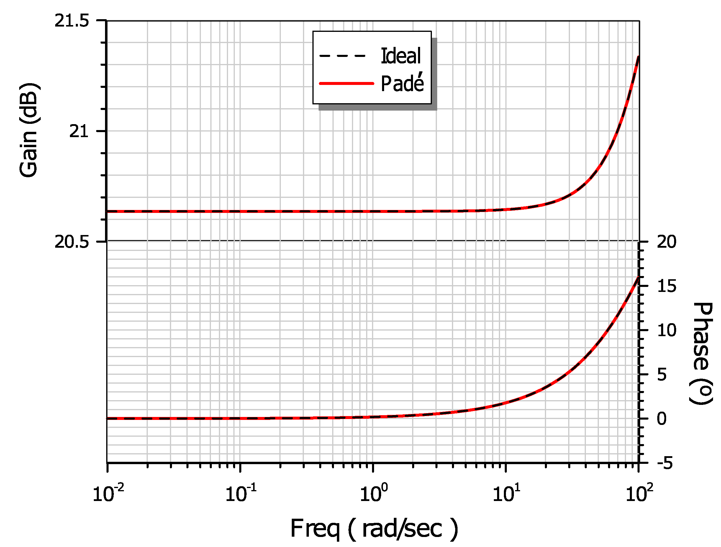
The gain and phase frequency responses obtained from (17), along with theoretically predicted ones given by dashes, are depicted in the plots of Figure 1, where the efficiency of the Padé approximation is readily obtained. The rational integer-order transfer function in (17) can be implemented by following well-known filter design techniques, including series (e.g., multifeedback schemes) as well the parallel connection of fundamental filter functions. The presented concept is general, in the sense that it is independent of the parameters of the FO-[PD] controller, and from the type of the employed plant, it offers versatility from an implementation point of view.
3. Implementation Aspects
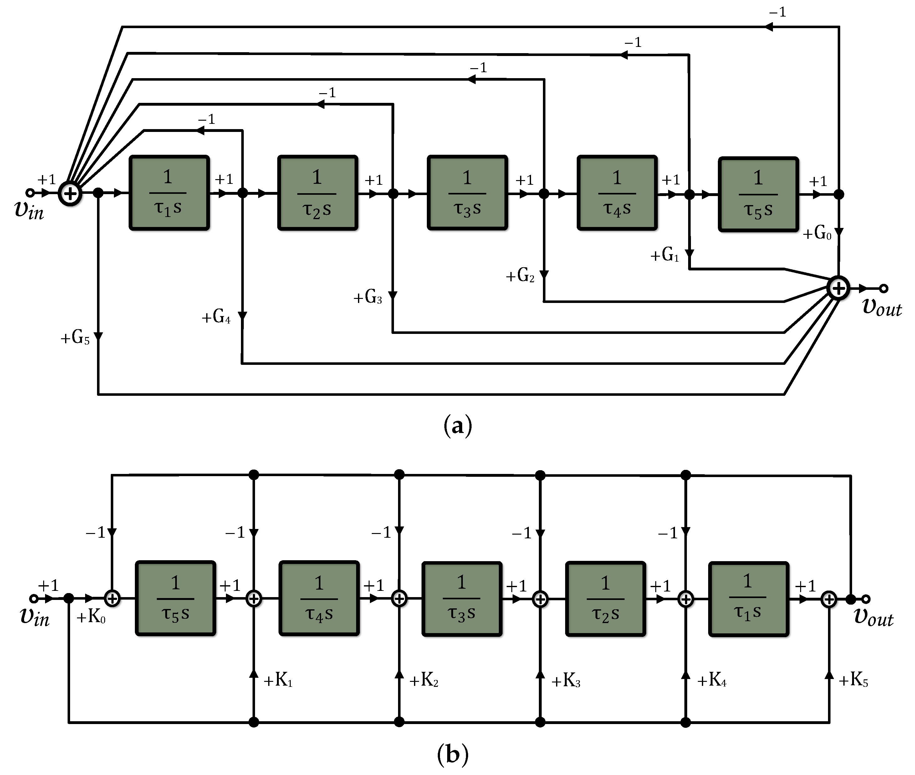
Multifeedback structures, such as follow-the-leader feedback (FLF) and inverse follow-the-leader feedback (IFLF), are extremely useful tools to describe these approximations and constitute the implementation of a generalized filter structure [33]. The functional block diagrams (FBDs) in Figure 2 represent these topologies for 5th-order approximation, which are described by the same transfer function as that given by (18)
where variables and represent scaling factors and time constants, respectively.
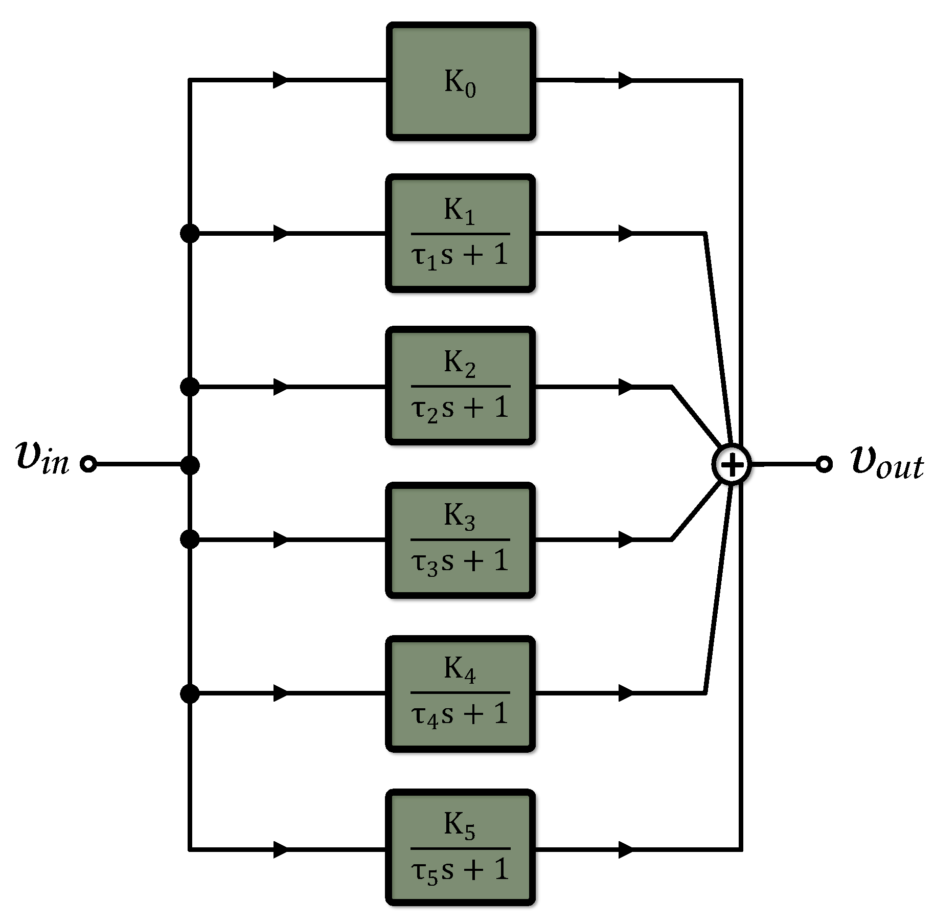
An alternative realization is based on the partial fraction expansion (PFE) of the transfer function in (17), and the obtained expression is the following:
with scaling factors and time constants given by the formulae: and , where and () are the residues and poles of the transfer function in (17) and [34]. The corresponding FBD is given in Figure 3.
The IFLF topology is more advantageous in terms of active component count than the FLF is in the case that active elements with differential input are utilized [35]. In this work, operational transconductance amplifiers (OTAs) are employed; therefore, the IFLF topology is compared with the corresponding PFE topology. Using (17)–(19), the values of scaling factors and time constants are summarized in Table 3.
The spread (i.e., the ratio of the maximal and minimal values of a variable) of the values of the variables in Table 3 is an important performance factor that affects total silicon area and/or power dissipation. The provided results show that the values of the spread of time-constants and scaling factors in the case of the IFLF topology are equal to 138.13 and 11.52, respectively. The corresponding values in the case of the PFE topology are 46.75 and 729.41. Taking into account that the time constants in OTA-C topologies are implemented as , where is the transconductance of the OTA [35], it is obvious that the spread of time constants affects the total capacitor occupied area. In addition, scaling factors in OTA-C topologies are implemented through an appropriate scaling of DC bias currents of OTAs; consequently, the spread of scaling factors affects the total power dissipation of the circuit. Therefore, the IFLF is preferable in the case where power dissipation must be minimized as it offers about 73 times lower maximal current, while the PFE is the best choice in the case of a system with minimal total capacitor area, as it requires three times lower maximal capacitance. Just for demonstration purposes, the performance of the IFLF topology is evaluated in the next section.
4. Simulation Results
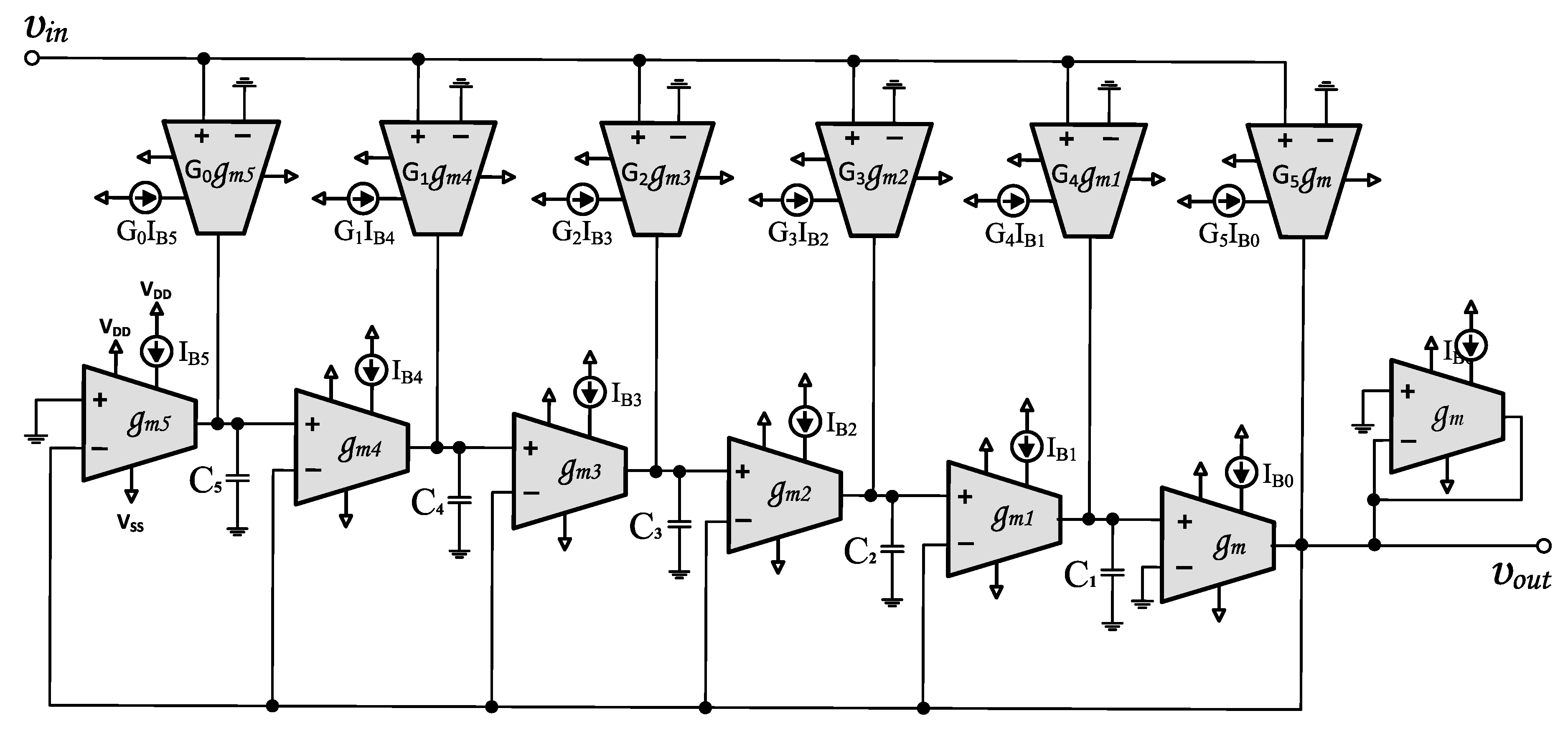
The OTA-C topology that implements the FBD in Figure 2b is demonstrated in Figure 4. An appropriate CMOS OTA topology in terms of linearity is demonstrated in [36] (Figure 5). Considering MOS transistors biased in the subthreshold region, realized transconductance is equal to , where is the bias current, is the subthreshold slope factor, and (≃26 mV at 27 °C) is thermal voltage. The time constants that are implemented following the design equation are given by
According to (20) the time constants are electronically adjustable, taking into account that scaling factors for IFLF method and for PFE method can be realized through the scaling of transconductances, which is also performed through a scaling of the corresponding bias currents.
The performance of the proposed fractional-order controller realizations were evaluated using the Cadence IC design suite and the MOS transistor models provided by the AMS 0.35 μm CMOS Design Kit. Power supply voltages are V. Assuming operation of the MOS transistors in the subthreshold region, their chosen aspect ratios are given in Table 4. The values of bias currents and of capacitors, derived using the content of Table 3, are provided in Table 5.
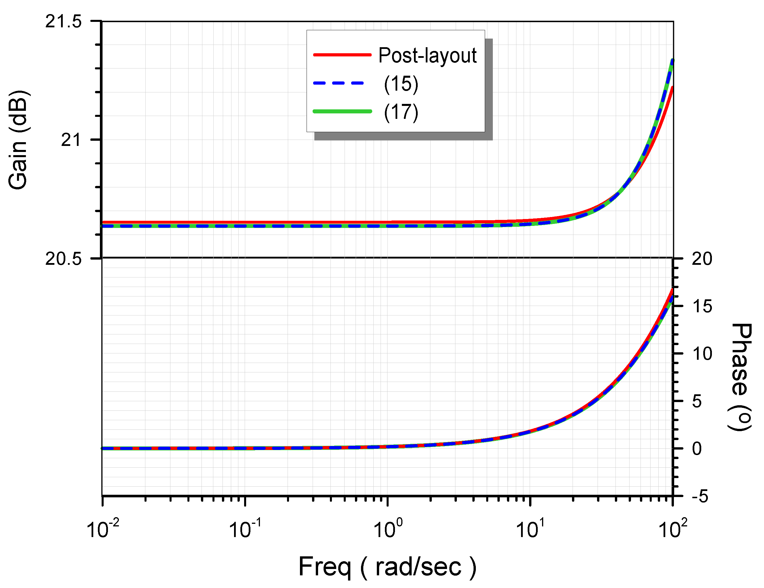
The layout of the controller was designed using the Virtuoso Layout Editor and is depicted in Figure 5, with the dimensions of 190.55 μm × 174.98 μm. The post-layout gain and phase responses of the controller, along with those derived from (15) and those derived from (17), are demonstrated in Figure 6.
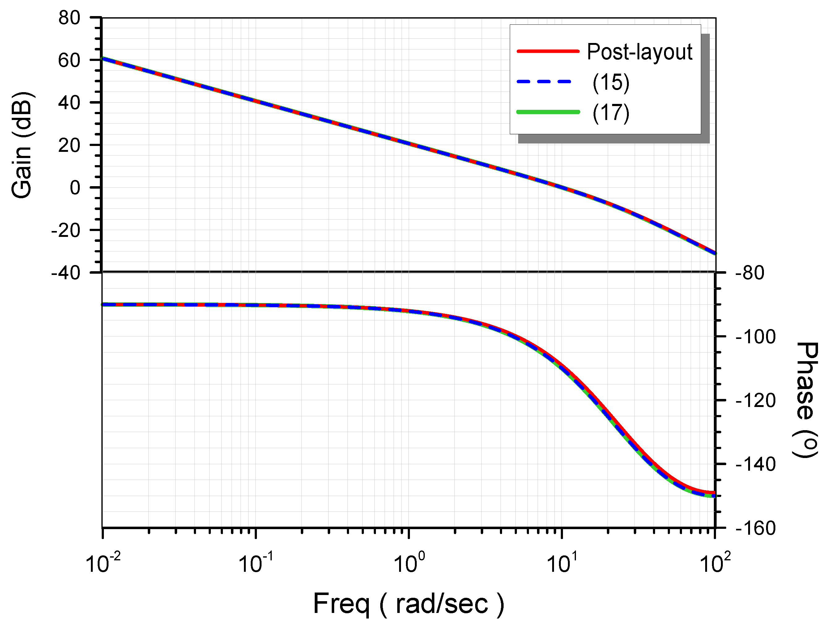
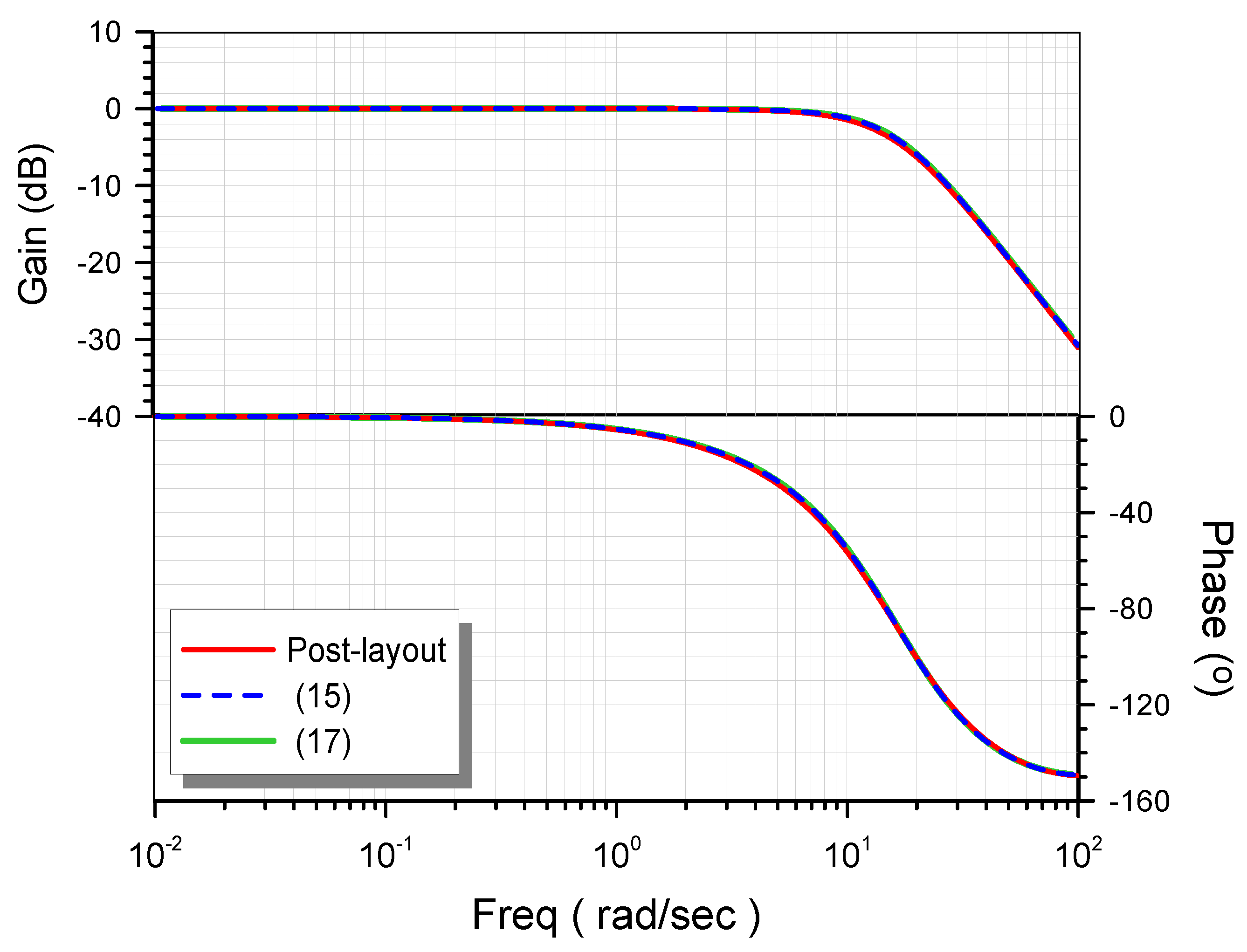
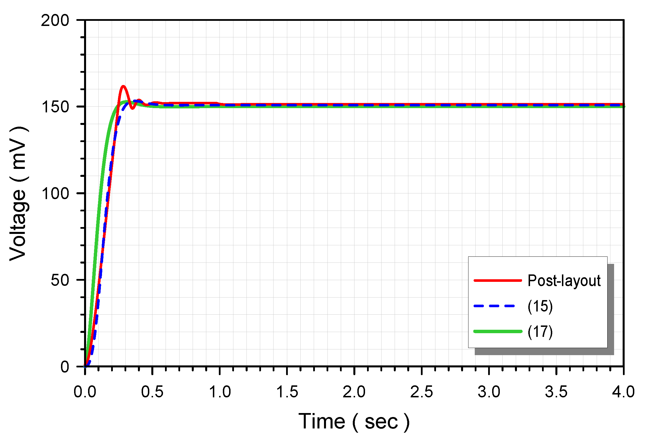
The corresponding open- and closed-loop responses of the controller–plant system are given in Figure 7 and Figure 8, respectively. The time-domain behavior was evaluated through the stimulation of the system by a 150 mV step signal, and the waveforms of the corresponding outputs are depicted in Figure 9.
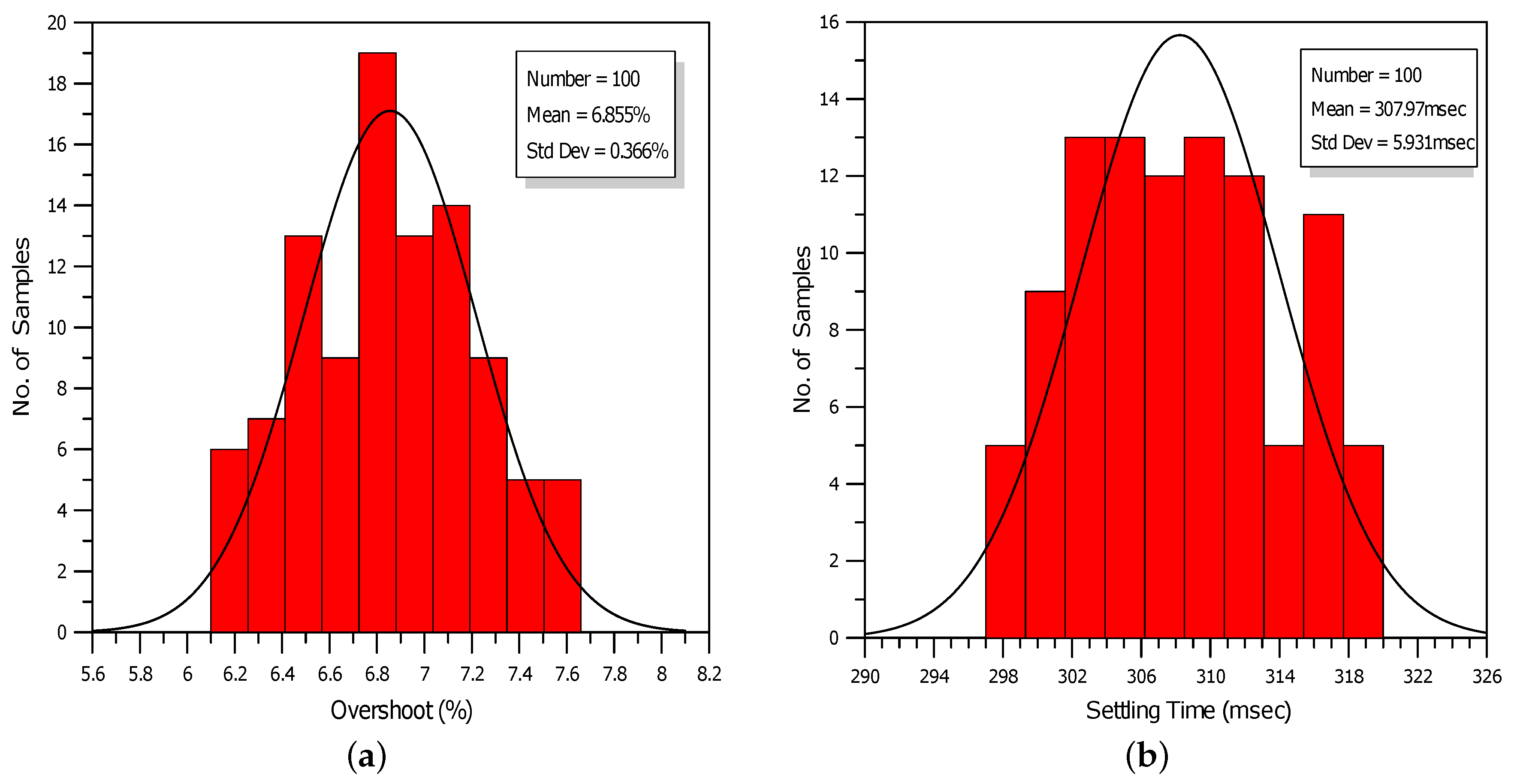
The robustness of the system was evaluated through Monte Carlo analysis offered by the Analog Design Environment for 100 runs. Considering the effects of MOS transistor parameters mismatching and process-parameter variations, the derived histograms related to the overshoot and settling time are given in Figure 10a,b, respectively. The values of the standard deviation were 0.366% and 5.931 ms with the corresponding mean values being 6.855% and 307.97 ms. The most important performance factors are summarized in Table 6, where the observed deviations in the time-step performance were mainly caused by the nonlinearity imposed by the OTA when it was leaving the small signal operation region.
5. Conclusions
The utilization of the Padé approximation solves the problem of the analog implementation of FO-[PD] controllers. The provided design example, where such a controller was employed in a motion-control system, showed that a high level of accuracy with regards to controller characteristics was achieved in both the frequency and the time domain. The main benefit of the proposed procedure is that it is general, in the sense that it is independent from specific controller characteristics and plant type. Another important aspect is the offered flexibility on the choice of the topology that could be utilized for implementing the derived integer-order transfer function. Choosing active elements with electronically controlled characteristics, such as OTAs, the resulting controller topology is fully adjustable and versatile because the characteristics of the controller are tuned through appropriate DC bias currents. On the other hand, in the case in which a controller with predefined characteristics must be designed, the employment of op-amp-based RC filter topologies is a cheaper solution [9,22]. Another attractive solution that combines an easy design procedure with programmability and versatility is the utilization of field-programmable analog arrays (FPAAs), which are based on configurable analog blocks (CABs) connected through programmable interconnects [37,38].
Author Contributions
Conceptualization, C.P. and A.S.E.; methodology, S.K.; software, R.M.; validation, R.M. and S.K.; formal analysis, C.P.; investigation, C.P., S.K. and A.S.E.; writing—original-draft preparation, R.M. and S.K.; writing—review and editing, C.P., A.S.E.; project administration, C.P. All authors have read and agreed to the published version of the manuscript.
Funding
This research received no external funding.
Data Availability Statement
No new data were created or analyzed in this study. Data sharing is not applicable to this article.
Acknowledgments
This research was cofinanced by Greece and the European Union (European Social Fund-ESF) through Operational Program “Human Resources Development, Education and Lifelong Learning” in the context of the project “Strengthening Human Resources Research Potential via Doctorate Research-2nd Cycle” (MIS-5000432), implemented by the State Scholarships Foundation (IKY).
Conflicts of Interest
The authors declare no conflict of interest.
Abbreviations
The following abbreviations are used in this manuscript:
| CMOS | Complementary metal oxide semiconductor |
| FO | Fractional order |
| FBD | Functional block diagram |
| FLF | Follow-the-leader feedback |
| IFLF | Inverse follow-the-leader feedback |
| IC | Integrated circuits |
| IO | Integer order |
| OTA | Operational transconductance amplifier |
| PFE | Partial fraction expansion |
| PID | Proportional integral derivative |
References
- Podlubny, I. Fractional-order systems and PIλDμ controllers. IEEE Trans. Autom. Control 1999, 44, 208–214. [Google Scholar] [CrossRef]
- Podlubny, I.; Petraš, I.; Vinagre, B.M.; O’leary, P.; Dorčák, L. Analogue realizations of fractional-order controllers. Nonlinear Dyn. 2002, 29, 281–296. [Google Scholar] [CrossRef]
- Vinagre, B.M.; Monje, C.A.; Calderón, A.J.; Suárez, J.I. Fractional PID controllers for industry application. A brief introduction. J. Vib. Control 2007, 13, 1419–1429. [Google Scholar] [CrossRef]
- Petráš, I. Fractional-Order Nonlinear Systems; Springer: Berlin, Germany, 2011. [Google Scholar]
- Monje, C.A.; Chen, Y.; Vinagre, B.M.; Xue, D.; Feliu-Batlle, V. Fractional-Order Systems and Controls: Fundamentals and Applications; Springer Science and Business Media: Berlin, Germany, 2010. [Google Scholar]
- Caponetto, R. Fractional Order Systems: Modeling and Control Applications; World Scientific: Singapore, 2010; Volume 72. [Google Scholar]
- Gonzalez, E.; Dorčák, L.; Monje, C.; Valsa, J.; Caluyo, F.; Petráš, I. Conceptual design of a selectable fractional-order differentiator for industrial applications. Fract. Calc. Appl. Anal. 2014, 17, 697–716. [Google Scholar] [CrossRef] [Green Version]
- Dimeas, I.; Petras, I.; Psychalinos, C. New analog implementation technique for fractional-order controller: A DC motor control. AEU-Int. J. Electron. Commun. 2017, 78, 192–200. [Google Scholar] [CrossRef]
- Muñiz-Montero, C.; García-Jiménez, L.V.; Sánchez-Gaspariano, L.A.; Sánchez-López, C.; González-Díaz, V.R.; Tlelo-Cuautle, E. New alternatives for analog implementation of fractional-order integrators, differentiators and PID controllers based on integer-order integrators. Nonlinear Dyn. 2017, 90, 241–256. [Google Scholar] [CrossRef]
- Kapoulea, S.; Psychalinos, C.; Elwakil, A.S. Single active element implementation of fractional-order differentiators and integrators. AEU-Int. J. Electron. Commun. 2018, 97, 6–15. [Google Scholar] [CrossRef]
- Kapoulea, S.; Tsirimokou, G.; Psychalinos, C.; Elwakil, A. OTA-C Implementation of Fractional-Order Lead/Lag Compensators. In Proceedings of the 2019 Novel Intelligent and Leading Emerging Sciences Conference (NILES), Giza, Egypt, 28–30 October 2019; Volume 1, pp. 38–41. [Google Scholar]
- Krijnen, M.E.; van Ostayen, R.A.; HosseinNia, H. The application of fractional order control for an air-based contactless actuation system. ISA Trans. 2018, 82, 172–183. [Google Scholar] [CrossRef] [Green Version]
- van Duist, L.; van der Gugten, G.; Toten, D.; Saikumar, N.; HosseinNia, H. FLOreS-Fractional order loop shaping MATLAB toolbox. IFAC-PapersOnLine 2018, 51, 545–550. [Google Scholar] [CrossRef]
- Dastjerdi, A.A.; Vinagre, B.M.; Chen, Y.; HosseinNia, S.H. Linear fractional order controllers; A survey in the frequency domain. Annu. Rev. Control 2019, 47, 51–70. [Google Scholar] [CrossRef]
- Psychalinos, C. Development of fractional-order analog integrated controllers–application examples. In Applications in Control; De Gruyter: Berlin, Germany, 2019; p. 357. [Google Scholar]
- Talebi, S.P.; Werner, S.; Li, S.; Mandic, D.P. Tracking dynamic systems in α-stable environments. In Proceedings of the ICASSP 2019—2019 IEEE International Conference on Acoustics, Speech and Signal Processing (ICASSP), Brighton, UK, 12–17 May 2019; pp. 4853–4857. [Google Scholar]
- Kapoulea, S.; Bizonis, V.; Bertsias, P.; Psychalinos, C.; Elwakil, A.; Petráš, I. Reduced Active Components Count Electronically Adjustable Fractional-Order Controllers: Two Design Examples. Electronics 2020, 9, 63. [Google Scholar] [CrossRef] [Green Version]
- Bauer, W.; Baranowski, J. Fractional PIλD Controller Design for a Magnetic Levitation System. Electronics 2020, 9, 2135. [Google Scholar] [CrossRef]
- Tepljakov, A.; Alagoz, B.B.; Yeroglu, C.; Gonzalez, E.; HosseinNia, S.H.; Petlenkov, E. FOPID controllers and their industrial applications: A survey of recent results. IFAC-PapersOnLine 2018, 51, 25–30. [Google Scholar] [CrossRef]
- Luo, Y.; Chen, Y. Fractional-order [proportional derivative] controller for robust motion control: Tuning procedure and validation. In Proceedings of the 2009 American Control Conference, St. Louis, MO, USA, 10–12 June 2009; pp. 1412–1417. [Google Scholar]
- Luo, Y.; Chen, Y. Fractional Order Motion Controls; Wiley Online Library: Hoboken, NJ, USA, 2012. [Google Scholar]
- Petráš, I. Handbook of Fractional Calculus with Applications: Vol. 6: Applications in Control; Walter de Gruyter GmbH & Co KG: Berlin, Germany, 2019. [Google Scholar]
- HosseinNia, S.H.; Saikumar, N. Fractional-order Precision Motion Control for Mechatronic Applications. In Handbook of Fractional Calculus with Applications; Petráš, I., Ed.; Walter de Gruyter GmbH & Co KG: Berlin, Germany, 2019; Volume 6, pp. 339–356. [Google Scholar]
- Luo, Y.; Chen, Y.; Pi, Y. Experimental study of fractional order proportional derivative controller synthesis for fractional order systems. Mechatronics 2011, 21, 204–214. [Google Scholar] [CrossRef]
- Malek, H.; Luo, Y.; Chen, Y. Identification and tuning fractional order proportional integral controllers for time delayed systems with a fractional pole. Mechatronics 2013, 23, 746–754. [Google Scholar] [CrossRef]
- Krishna, B.T. Studies on fractional order differentiators and integrators: A survey. Signal Process. 2011, 91, 386–426. [Google Scholar] [CrossRef]
- Oustaloup, A.; Levron, F.; Mathieu, B.; Nanot, F.M. Frequency-band complex noninteger differentiator: Characterization and synthesis. IEEE Trans. Circuits Syst. I Fundam. Theory Appl. 2000, 47, 25–39. [Google Scholar] [CrossRef]
- Tavazoei, M.S.; Tavakoli-Kakhki, M. Compensation by fractional-order phase-lead/lag compensators. IET Control Theory Appl. 2014, 8, 319–329. [Google Scholar] [CrossRef]
- Lanusse, P.; Sabatier, J.; Gruel, D.N.; Oustaloup, A. Second and third generation CRONE control-system design. In Fractional Order Differentiation and Robust Control Design; Springer: Dordrecht, The Netherlands, 2015; pp. 107–192. [Google Scholar]
- Xue, D. Fractional-Order Control Systems: Fundamentals and Numerical Implementations; Walter de Gruyter GmbH & Co KG: Berlin, Germany, 2017; Volume 1. [Google Scholar]
- Bošković, M.Č.; Rapaić, M.R.; Šekara, T.B.; Mandić, P.D.; Lazarević, M.P.; Cvetković, B.; Lutovac, B.; Daković, M. On the rational representation of fractional order lead compensator using Padé approximation. In Proceedings of the 2018 7th Mediterranean Conference on Embedded Computing (MECO), Budva, Montenegro, 10–14 June 2018; pp. 1–4. [Google Scholar]
- Kapoulea, S.; Tsirimokou, G.; Psychalinos, C.; Elwakil, A.S. Employment of the Padé Approximation for Implementing Fractional-Order Lead/Lag Compensators. AEU-Int. J. Electron. Commun. 2020, 120, 153203. [Google Scholar] [CrossRef]
- Tsirimokou, G.; Psychalinos, C.; Elwakil, A. Design of CMOS Analog Integrated Fractional-Order Circuits: Applications in Medicine and Biology; Springer: Cham, Switzerland, 2017. [Google Scholar]
- Bertsias, P.; Psychalinos, C.; Maundy, B.J.; Elwakil, A.S.; Radwan, A.G. Partial fraction expansion—Based realizations of fractional-order differentiators and integrators using active filters. Int. J. Circuit Theory Appl. 2019, 47, 513–531. [Google Scholar] [CrossRef]
- Mohan, P.A. VLSI Analog Filters: Active RC, OTA-C, and SC; Springer Science and Business Media: Berlin, Germany, 2012. [Google Scholar]
- Tsirimokou, G.; Psychalinos, C.; Elwakil, A.S. Emulation of a constant phase element using operational transconductance amplifiers. Analog Integr. Circuits Signal Process. 2015, 85, 413–423. [Google Scholar] [CrossRef]
- Muñiz-Montero, C.; Sánchez-Gaspariano, L.A.; Sánchez-López, C.; González-Díaz, V.R.; Tlelo-Cuautle, E. On the electronic realizations of fractional-order phase-lead-lag compensators with OpAmps and FPAAs. In Fractional Order Control and Synchronization of Chaotic Systems; Springer: Cham, Switzerland, 2017; pp. 131–164. [Google Scholar]
- Tlelo-Cuautle, E.; Pano-Azucena, A.D.; Guillén-Fernández, O.; Silva-Juárez, A. Analog/Digital Implementation of Fractional Order Chaotic Circuits and Applications; Springer: Cham, Switzerland, 2020. [Google Scholar]
Figure 1.
Approximated controller gain and phase frequency responses derived according to (17).
Figure 1.
Approximated controller gain and phase frequency responses derived according to (17).

Figure 2.
Functional block diagrams of 5th-order (a) FLF and (b) IFLF topologies.

Figure 3.
Functional block diagram of 5th–order PFE topology.

Figure 4.
5th–order IFLF filter topology using OTAs.

Figure 5.
Layout design of the proposed controller.

Figure 6.
Post-layout gain and phase frequency responses of the controller.

Figure 7.
Post-layout open-loop gain and phase-frequency responses of the system (controller-plant).
Figure 7.
Post-layout open-loop gain and phase-frequency responses of the system (controller-plant).

Figure 8.
Post-layout closed-loop gain and phase frequency responses of the system (controller-plant).
Figure 8.
Post-layout closed-loop gain and phase frequency responses of the system (controller-plant).

Figure 9.
Post-layout step-response of the closed-loop system stimulated by a step input voltage 150 mV.
Figure 9.
Post-layout step-response of the closed-loop system stimulated by a step input voltage 150 mV.

Figure 10.
Histogram plots of (a) overshoot and (b) settling time of open-loop system (controller-plant).
Figure 10.
Histogram plots of (a) overshoot and (b) settling time of open-loop system (controller-plant).


Table 1.
Main subcategories of FO-PID controllers employed in motion-control systems.
| Type of Controller | Order | Transfer Function |
|---|---|---|
| FO-PI | ||
| FO-[PI] | ||
| FO-PD | ||
| FO-[PD] |
| Coefficient | Value | Coefficient | Value |
|---|---|---|---|
| 124 | – | – |
Table 3.
Values of time constants and scaling factors for IFLF and PFE topology implementations.
| IFLF | PFE | ||
|---|---|---|---|
| Variable | Value | Variable | Value |
| 124 | |||
| 124 | |||
| (ms) | (ms) | ||
| (ms) | (ms) | ||
| (ms) | (ms) | ||
| (ms) | (ms) | ||
| (ms) | (ms) | ||
| Transistor | Aspect Ratio () |
|---|---|
| – | 5/15 μm/μm |
| , | 10/5 μm/μm |
| – | 2/5 μm/μm |
| – | 1/8 μm/μm |
Table 5.
Values of bias currents and capacitors in the OTA-C topology in Figure 4.
Table 5.
Values of bias currents and capacitors in the OTA-C topology in Figure 4.
| Bias Current | Value | Capacitor | Value |
|---|---|---|---|
| 392.2 pA | – | – | |
| 597.5 pA | 0.886 pF | ||
| 107.8 pA | 1.15 pF | ||
| 31.13 pA | 1.01 pF | ||
| 34.0 pA | 2.52 pF | ||
| 32.4 pA | 7.30 pF |
Table 6.
Comparison of derived phase-margin, overshoot, settling-time, and rise-time values.
| System | Phase Margin | Overshoot | Settling Time | Rise Time |
|---|---|---|---|---|
| Ideal | 70.00° | 1.621% | 256.1 ms | 164.3 ms |
| Post-layout | 70.86° | 6.866% | 308.2 ms | 178.0 ms |
Publisher’s Note: MDPI stays neutral with regard to jurisdictional claims in published maps and institutional affiliations. |
© 2021 by the authors. Licensee MDPI, Basel, Switzerland. This article is an open access article distributed under the terms and conditions of the Creative Commons Attribution (CC BY) license (https://creativecommons.org/licenses/by/4.0/).
Share and Cite
MDPI and ACS Style
Malatesta, R.; Kapoulea, S.; Psychalinos, C.; Elwakil, A.S. Design of Low-Voltage FO-[PD] Controller for Motion Systems. J. Low Power Electron. Appl. 2021, 11, 26. https://0-doi-org.brum.beds.ac.uk/10.3390/jlpea11020026
AMA Style
Malatesta R, Kapoulea S, Psychalinos C, Elwakil AS. Design of Low-Voltage FO-[PD] Controller for Motion Systems. Journal of Low Power Electronics and Applications. 2021; 11(2):26. https://0-doi-org.brum.beds.ac.uk/10.3390/jlpea11020026
Chicago/Turabian StyleMalatesta, Rafailia, Stavroula Kapoulea, Costas Psychalinos, and Ahmed S. Elwakil. 2021. "Design of Low-Voltage FO-[PD] Controller for Motion Systems" Journal of Low Power Electronics and Applications 11, no. 2: 26. https://0-doi-org.brum.beds.ac.uk/10.3390/jlpea11020026
Note that from the first issue of 2016, this journal uses article numbers instead of page numbers. See further details here.