
Low-Power FPGA Architecture Based Monitoring Applications in Precision Agriculture


1
Laboratory of Systems Engineering and Information Technology LISTI, National School of Applied Sciences, Ibn Zohr University, Agadir 80000, Morocco
2
SATIE, ENS, Paris-Saclay University, 91190 Gif-sur-Yvette, France
*
Author to whom correspondence should be addressed.
J. Low Power Electron. Appl. 2021, 11(4), 39; https://0-doi-org.brum.beds.ac.uk/10.3390/jlpea11040039
Submission received: 23 August 2021
/
Revised: 22 September 2021
/
Accepted: 27 September 2021
/
Published: 30 September 2021
(This article belongs to the Special Issue Advanced Researches in Embedded Systems)
Abstract
:Today’s on-chip systems technology has grounded impressive advances in computing power and energy consumption. The choice of the right architecture depends on the application. In our case, we were studying vegetation monitoring algorithms in precision agriculture. This study presents a system based on a monitoring algorithm for agricultural fields, an electronic architecture based on a CPU-FPGA SoC system and the OpenCL parallel programming paradigm. We focused our study on our own dataset of agricultural fields to validate the results. The fields studied in our case are in the Guelmin-Oued noun region in the south of Morocco. These fields are divided into two areas, with a total surface of 3.44 Ha2 for the first field and 3.73 Ha2 for the second. The images were collected using a DJI-type unmanned aerial vehicle and an RGB camera. Performance evaluation showed that the system could process up to 86 fps versus 12 fps or 20 fps in C/C++ and OpenMP implementations, respectively. Software optimizations have increased the performance to 107 fps, which meets real-time constraints.
1. Introduction
Algorithm-based vegetation indices monitoring involves mathematical models used in precision agriculture. The main role of these indices is to extract information used on agricultural fields. This information will be interpreted later to monitor the crop in the agricultural areas. The use of embedded systems in the field of monitoring has been increasing. As a solution proposed in the literature, we can find applications based on embedded CPU systems, such as raspberry [1], and CPU-GPU systems, such as the jetson family proposed by NVIDIA [2].
Due to the processing power used in GPU architectures, these architectures can be strong options for implementing monitoring algorithms. However, the problem with this type of architecture is the high energy consumption, limiting the use of autonomous systems such as robots and unmanned aerial vehicles. As a solution, we address the use of FPGA architectures; this type of architecture combines computational power and energy savings [3,4].
On-chip FPGA systems contain a CPU and an FPGA coprocessor; this heterogeneous system helps to speed up processing by focusing on reducing processing time and energy consumption. This type of system can help us in cases where we have agricultural fields with a huge surface. The autonomous monitoring of this type of field based on UAVs or robots requires the use of low-cost systems as well as low energy consumption [5]. In the context of monitoring indices in agricultural fields, the literature offers various indices based on different special bands depending on the application. We can divide these indices into three families. The first family is based on hyperspectral bands such as the moisture index [6,7]. The second type is based on the vegetation and water index; this type of index uses multispectral images [8]. The last type is based on RGB images; this index represents low-cost solutions based on RGB cameras instead of expensive multispectral or hyperspectral cameras [9].
In our work, we aim to accelerate the processing of indices for real-time applications on heterogeneous CPU-FPGA systems, as well as to study the implementation issues and the corresponding optimizations. The results have been evaluated on real datasets based on a DJI UAV and an RGB camera [8].
Our contribution is as follows:
- Speeding up the algorithm proposed in [8] for indices computation on a CPU-FPGA-based SoC using the OpenCL paradigm;
- Design study of the proposed architecture based on the H/S Co-Design approach;
- A case study on a data set acquired on agricultural fields (Guelmim-Oued Noun region in the south of Morocco).
The rest of the paper is organized as follows:
We provide an overview of the different monitoring applications in agricultural fields. Subsequently, we present the two areas that will be used in our study. Afterward, the methodology followed will be explained, and the hardware and experimental implementation results will be discussed. Finally, we give a conclusion and an outline of future work.
2. Overview and Study Area
2.1. RGB Indices Overview in Precision Agriculture
Monitoring applications in agricultural fields aim to predict performance in the corresponding areas. This prediction is based on weed counts, weed detection, and other applications [10,11,12]. However, none of these applications can be realized if a disease-resistant crop is not detected. For this reason, the monitoring of vital signs plays a very important role in different applications. Several works have been developed towards monitoring agricultural fields based on various indices. In this context, L. Congcong et al. (2019) used the normalized difference vegetation index (NDVI) to monitor plant growth in real-time. The evaluation of the proposed approach was based on satellite images between 2018 and 2014 [13]. R. Shoujia et al. 2021 used NDVI for yield prediction in agricultural fields [14]. In [8], the authors used NDVI and the Normalized Difference Water Index (NDWI) to perform agricultural field analysis using an embedded CPU-GPU system.
In terms of monitoring indices based on multispectral cameras, NDVI and NDWI are the most widely used indices in the field, either for detecting diseases or for yield prediction and crop monitoring. However, RGB indices present an alternative solution to other indices that require multispectral and hyperspectral cameras. The problem with this type of camera is the high cost. Therefore, the construction of a low-cost system requires this type of solution, which is based on RGB cameras. Among the RGB indices, we can identify the Red Green Blue Vegetation Index (RGBVI), based on the three bands red, green and blue, proposed in [15]. Additionally, the Modified Green Red Vegetation Index (MGRVI) is an improvement of the Green Red Vegetation Index (GRVI) based on the two bands red and green [16].
Thus, we can find various applications in the agriculture field. These applications are based on different tools; e.g., R. Bezen et al. (2020) proposed a GPU-based system for cow feed intake measurement. The approach proposed by the authors is based on an RGB-D camera and the CNN model. After evaluation, they showed that the system processes the algorithm in real time for the developed application [17]. In the same way, J. Gené-Mola et al. (2019) proposed a method for Fuji apple detection based on an Nvidia TITAN GTX GPU system and the R-CNN approach. The tool used for image collection was a Kinect v2 RGB-D camera [18]. The embedded part was based on a raspberry V3 board. In addition, J. Shin et al. 2021 proposed a system based on an Intel workstation with a CPU operating at 3.2 GHz implemented in MATLAB. This system is dedicated to detecting disease in strawberry farms with an accuracy that can reach 92.61%. Table 1 summarizes the recent applications used in precision agriculture.
In our case, we chose the two indices Green Red Vegetation Index (GRVI) and Green Leaf Index (GLI). Both indices track and detect the vegetation in agricultural fields using RGB cameras. Equations (1) and (2) show how we can obtain these indices.
The values of these indices vary between −1 and 1. Generally, an index less than 0 reflects soil or non-living plants. Values above 0 reflect vegetation. Therefore, the threshold of these indices must be above 0 [28].
2.2. FPGA-SoC Architecture Overview
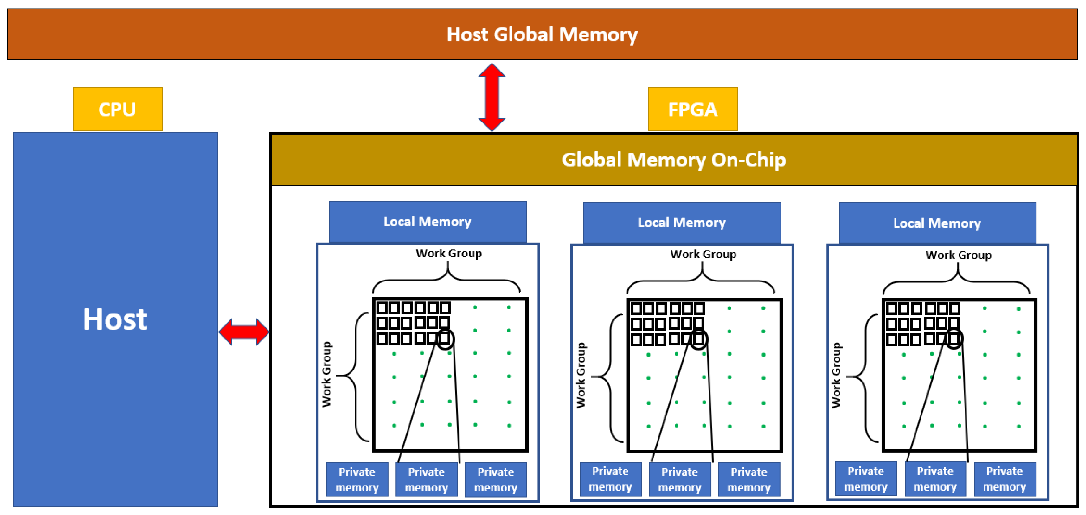
The architectures listed in Table 1 are based on GPU processors. The use of this type of architecture is due to the high computing power. However, the problem here is the high energy consumption, limiting the use of autonomous systems based on monitoring agricultural fields. The use of FPGA on-chip systems can solve this problem. Among the most reliable and robust systems in parallel processing are the CPU-FPGA systems, which contain both a CPU and an FPGA. Figure 1 shows the CPU-FPGA architecture. the host global memory is the memory of the CPU that contains the whole memory. The host is the CPU part of the board. Local memory is the device part (FPGA) memory, which shares the work with the items of each group. Global memory on-chip is the global memory of the FPGA part. The Work Group is a set of work items; the number of work items depends on the configuration chosen in the CPU part. The private memory is that which is not shared with the elements of each work group.
Generally, the exploitation of an FPGA architecture is achieved using VHSIC Hardware Description Language (VHDL) [29]. On the other hand, the CPU architecture is operated using languages such as C/C++. Therefore, using both parts (CPU and FPGA) simultaneously in the same architecture requires a high-level language such as OpenCL paradigm. OpenCL is a parallel programming language used to improve performance by exploiting the architecture as much as possible. It is a dedicated language for heterogeneous architectures that contains a host and a device part. Generally, the host part is a CPU, and the device can include GPU, FPGA, or DSP. In our case, we have opted for the CPU-FPGA architecture, given its computational performance as well as its low power consumption. The selected device in our study is the Cyclone V SoC, proposed by the Intel-Altera company. This on-chip system contains a Cyclone V FPGA with a hardware dual-core A9 cortex processor. Besides its low power consumption, this type of architecture is characterized by its low cost compared to other CPU-GPU architectures. Additionally, CPU-FPGA systems are characterized by their pseudo-parallel behavior in different processes. This makes this architecture the best choice.
Table 2 summarizes the different characteristics of the evaluation platform used.
We did not choose a CPU-GPU architecture because this architecture leads to a high energy consumption. Moreover, it uses the CUDA language, which is dedicated to Nvidia CPU-GPU architectures only, and no other architectures such as Intel or AMD. For this reason, OpenCL presents a flexible and powerful solution for the various architectures used.
2.3. Area Study
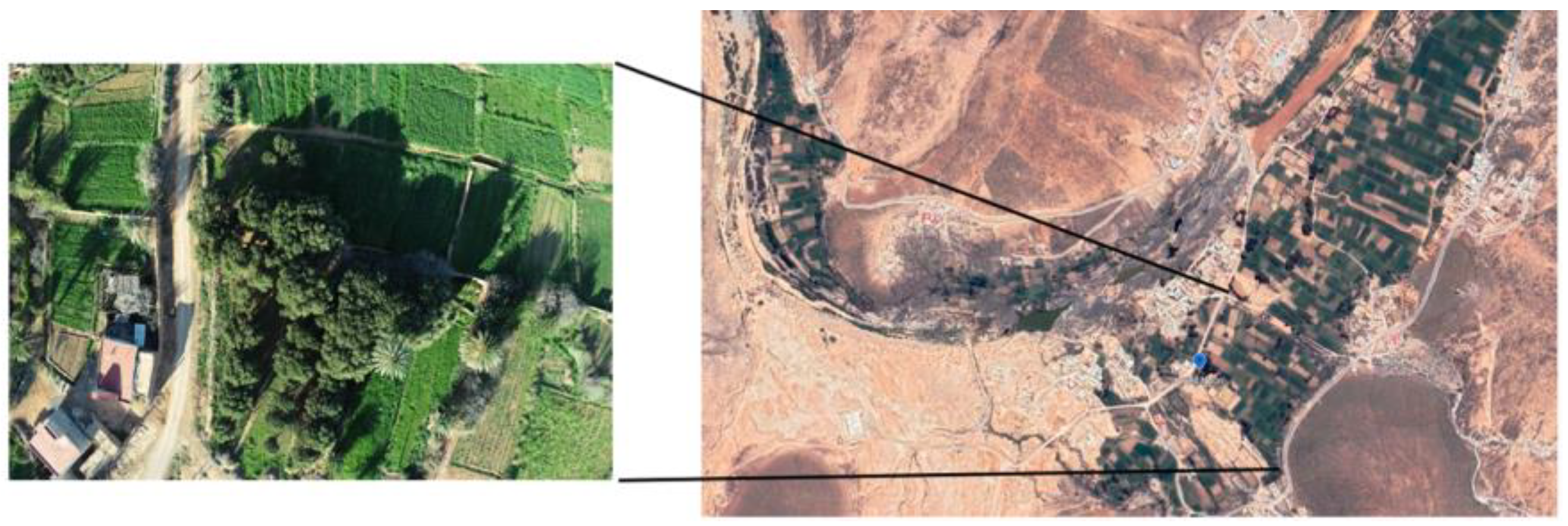
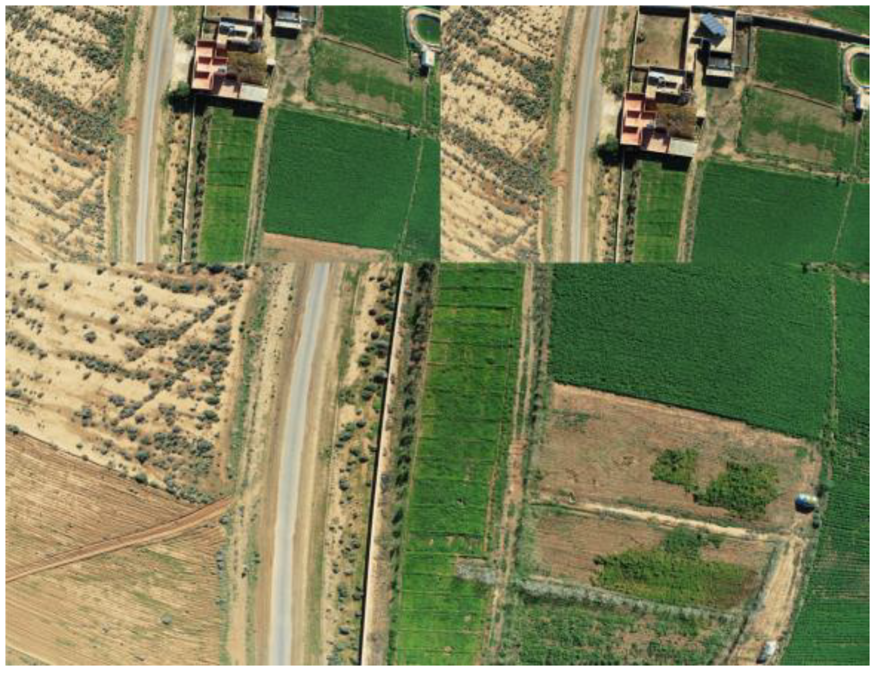
The agricultural field selected in our study is located in the Guelmim-Oued Noun region in the south of Morocco, with a perimeter of 0.81 Km and a surface area of 3.44 Ha2. The coordinates of the agricultural field used in this study are 29°04′39″ N and 10°16′29″ W. Thus, the tools used for collecting our dataset are based on an unmanned aerial vehicle type DJI Phantom Pro4 with an RGB camera based on 1-inch CMOS and 20 Mpx. The lens had an FOV of 84°8.8 mm/24 mm and a focal length f/2.8 auto focus. The left image of Figure 2 shows an example of images collected with the UAV.
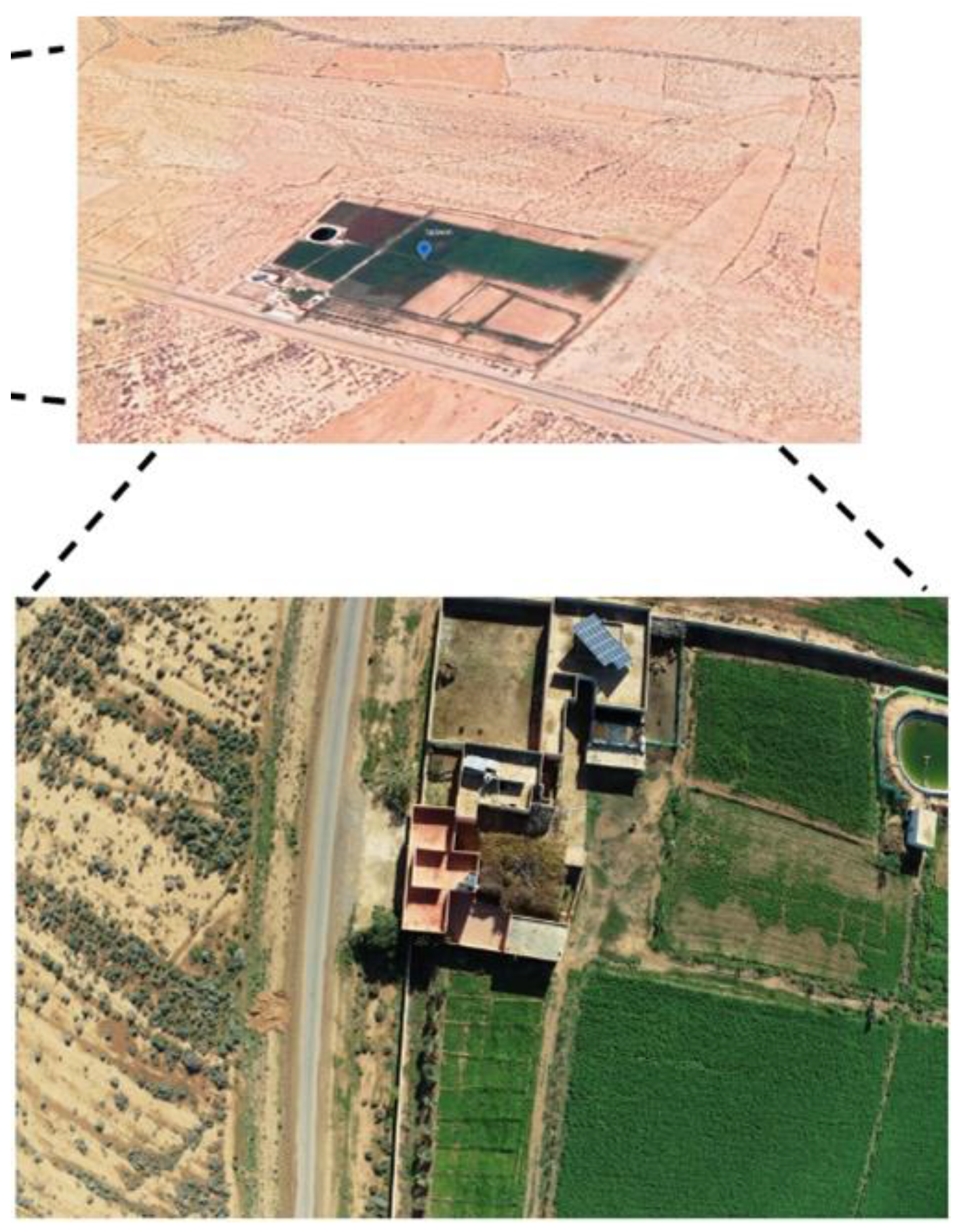
The type of camera used in this study operated on RGB bands. The reason for using this camera is the low cost of this type of sensor compared to multispectral cameras that operate on near-infrared or red-edge bands. In this study, we also used another field located in the Guelmim-Oued Noun region, with a longitude of 29°00′36″ N and a latitude of 10°12′39″ W. The selected field’s perimeter is about 0.78 Km, with a surface area of 3.73 Ha2. Figure 3 shows the localization of the second field.
3. Methodology and Results
3.1. Methodology
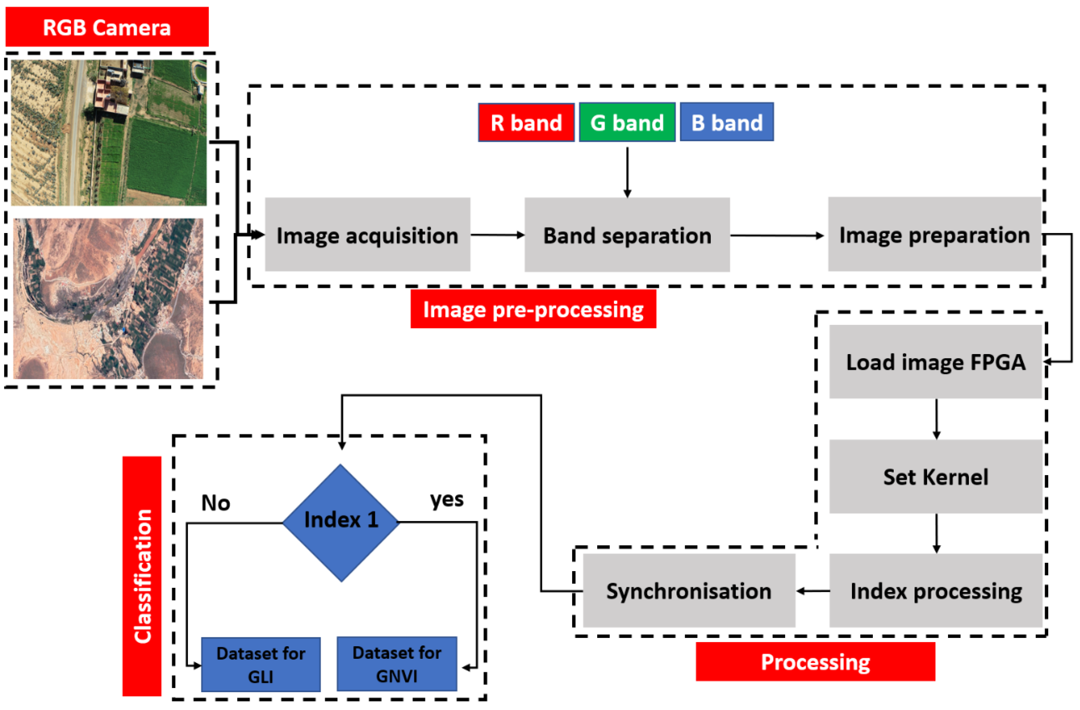
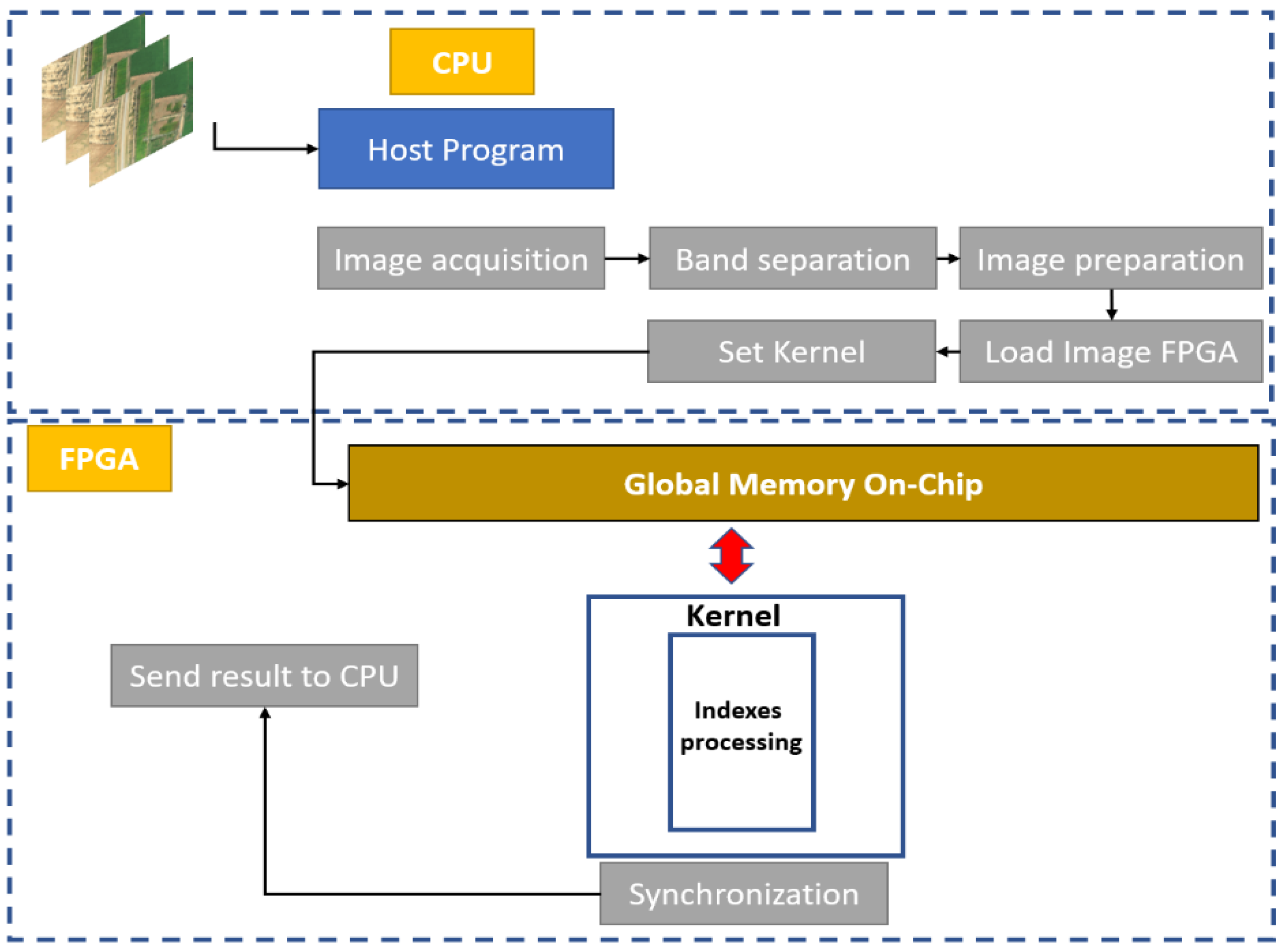
The methodology adopted in our study is based on a hardware–software partitioning and processing-time evaluation using the C/C++ language and OpenCl paradigm. A study was conducted to define parts that consume more time in order to be accelerated in the CPU-FPGA system. The developed code is based on two parts. The first one is dedicated to the CPU, which loads the necessary data for the FPGA coprocessor acceleration. For the device part, we used an Altera offline compiler (AOC) based on the OpenCL kernel. Then, we compiled our kernel to create the hardware part that was to be implemented in the FPGA part. The evaluation of the hardware constraint in our implementation was based on two techniques. The first one was to make the naive implementation in order to evaluate the performance. The second one was based on optimization using the local fast memory compared to the global memory. Figure 6 shows the algorithm we used for the implementation, and Figure 7 shows the naive implementation.
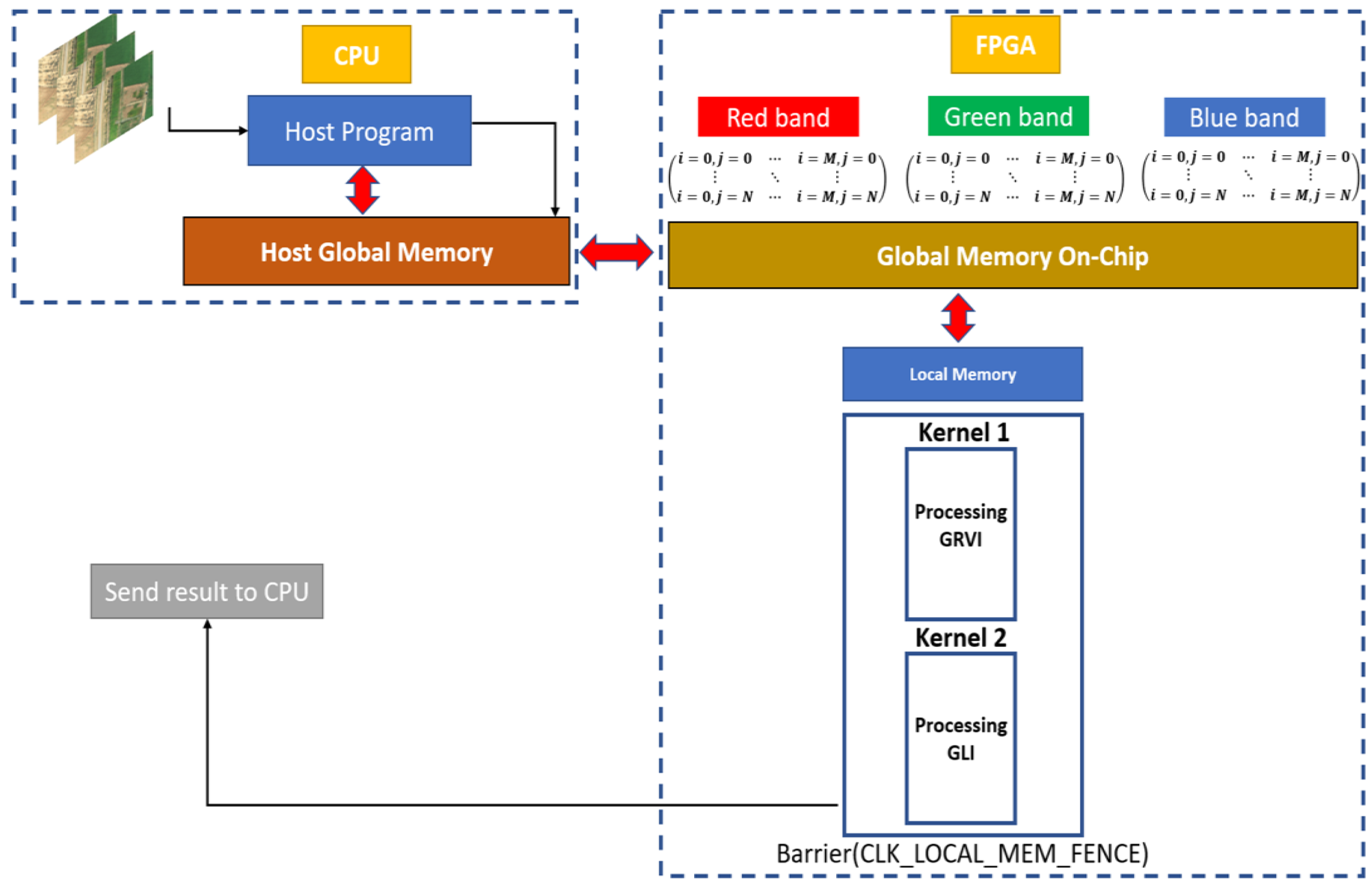
After the naive implementation in the CPU-FPGA architecture, we improved the processing time using the local memory of the FPGA board. Once we acquired the images, the data were uploaded to the FPGA global memory. The local memory was used for kernel processing. In addition, we used two kernels to avoid data concurrency. The first kernel was dedicated to processing the GRVI index, and the second one was dedicated to the GLI index. The evaluation has shown that the second technique gives better results than the first one in terms of processing times. Figure 8 shows the second technique used to improve the first implementation.
3.2. Processing Times Evaluation
We have evaluated the processing times between different implementations. As well as a comparison of two implementations (the first one using an intel desktop operating 2.2 GHz, the second one using an XU4 platform operative at 2 Ghz), both are CPU-GPU architectures. The XU4 platform is equipped with an Exynos 5 processor, which contains an ARM Cortex A7 and A15 with 1.4 Ghz and 2 Ghz, respectively, as well as a Mali T628MP6 GPU. For the TX1 platform, we used an ARM Cortex A57 MPCore processor and an Nvidia Maxwell GPU with 256 cores. Table 3 presents the specifications of the used platforms. Table 4 presents a synthesis of the different processing times obtained using different languages and architectures.
The processing time on the desktop allows us to process 32 fps (frames per second) based on C/C++ implementation. On the other hand, the use of the OpenMP directive leads to a rate of 66 fps. In the case of the XU4 platform, we can process 21 fps using OpenMP optimization, but only 12 fps in the case of C/C++ implementation. The TX1 platform gave us 80 ms for the sequential processing, and about 0.77 ms using the CUDA heterogeneous architecture programming language.
The time shown in Table 3 shows that the real-time constraint is respected in the case of the desktop using OpenMP, as well as in the case of the TX1 board using CUDA. The real-time constraint, in our case, is based on the acquisition frequency of the RGB camera. The camera used in our study operates at 60 fps. Therefore, it is necessary to follow this frequency in order to achieve real-time processing. Generally, desktops are not suitable because they are validation tools and not embedded architecture, and they consume more energy than an embedded architecture. Additionally, the TX1 card can present an alternative solution for boarding the various algorithms. This type of card also consumes a lot of energy—as much as 15 W—compared to the other embedded architectures.
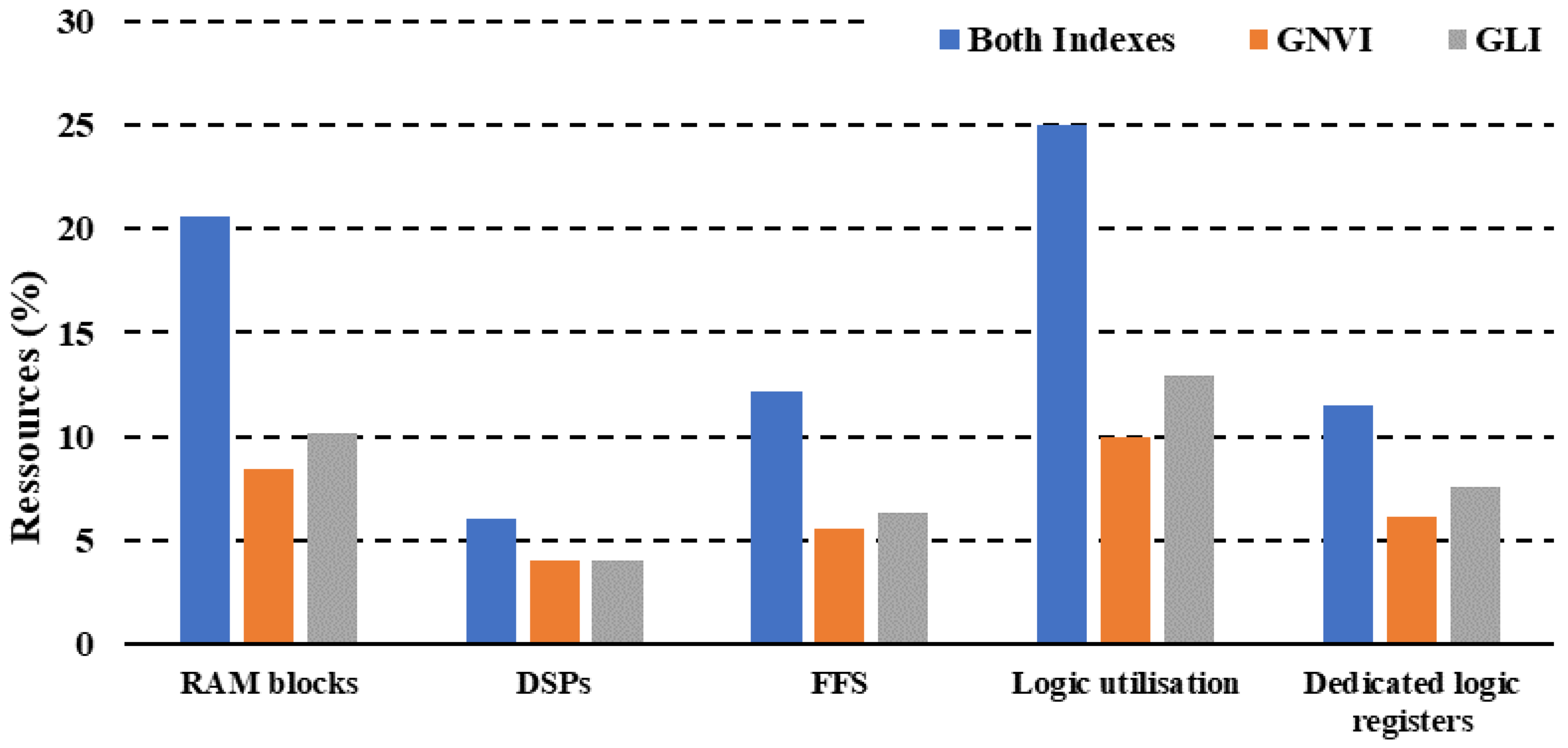
The solution is to use a low-cost system with low power consumption. The SoC system based on a CPU-FPGA architecture can present a robust solution for high processing efficiency and low power consumption. In our case, we have evaluated both implementations on the same platform. Figure 9 shows the results obtained after the synthesis and placement routing.
The evaluation of the resources shown in Figure 8 is based on the RAM (random access memory) blocks consumed, the DSP (digital signal processing), the FFS (flip flops), logic usage, and the dedicated logic register. The results show that the naive implementation based on processing two indices in the same kernel consumes 20.63% of RAM, 6% of DSPs, 12.15% of FFS, 25% logic usage, and 11.53% of the dedicated logic registers. On the other hand, the implementation based on two separated kernels and the use of the FPGA on-chip memory has significant benefits. This implementation achieved rates of 8.4% for the GNVI kernel and 10.2% for GLI in the RAM block utilization. The DSPs achieved 4% for the GNVI kernel and the same for the GLI kernel.
Additionally, FFS showed consumption rates of 5.56% and 6.32% for GNVI and GLI, respectively. In addition, logic usage was 10% for GNVI and 12.96% for GLI. We noticed that the GLI kernel consumed more resources than GNVI, due to the fact that the GLI index is based on three bands in place of two in the GNVI case, which leads to its higher consumption. Table 5 summarizes the different results obtained.
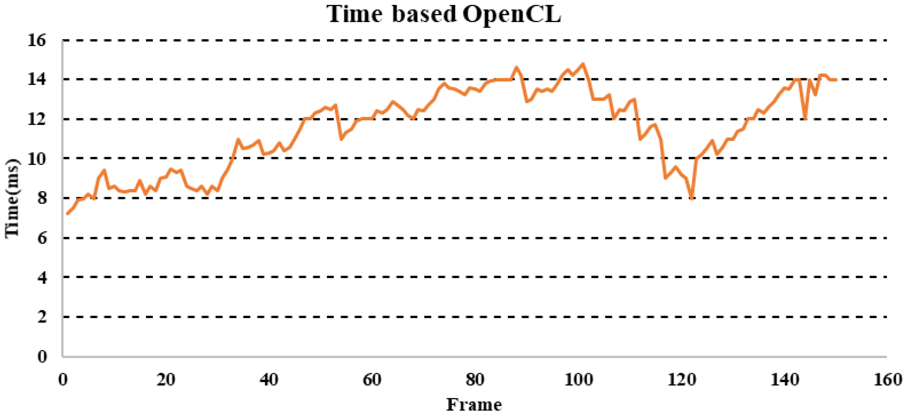
After the extraction of different resources, we proceeded to the processing time evaluation. This evaluation was based on a sequence of 150 images, evaluating the robustness of the processing task. Figure 10 shows the results obtained.
Figure 10 shows the results obtained with the evaluation of the algorithm used on an image sequence. The time varied between a minimum value of 7.23 ms and a maximum value of 14.8, with an average of 11.5 ms. The approach used in this work allowed us to accelerate the second block shown in Figure 6, which was based on the processing of indices. The sequential evaluation of processing time confirmed this choice, which encouraged us to process the first block in the CPU part (host) and the second block in the device part (FPGA) in order to return the results to the host for classification. In the proposed acceleration, we used a naive acceleration based on a single kernel that achieved all the processing. Subsequently, we optimized this implementation in terms of processing time by using the fast local memory of the CPU-FPGA architecture. The tool used in our case was based on OpenCL, both for the naive implementation and the optimized version. The following two pseudo codes (Algorithms 1 and 2) show the processing in the host part and the kernel part.
| Algorithm 1: Kernel Code |
Start Algorithm
|
| Algorithm 2: Host code |
Start Algorithm
|
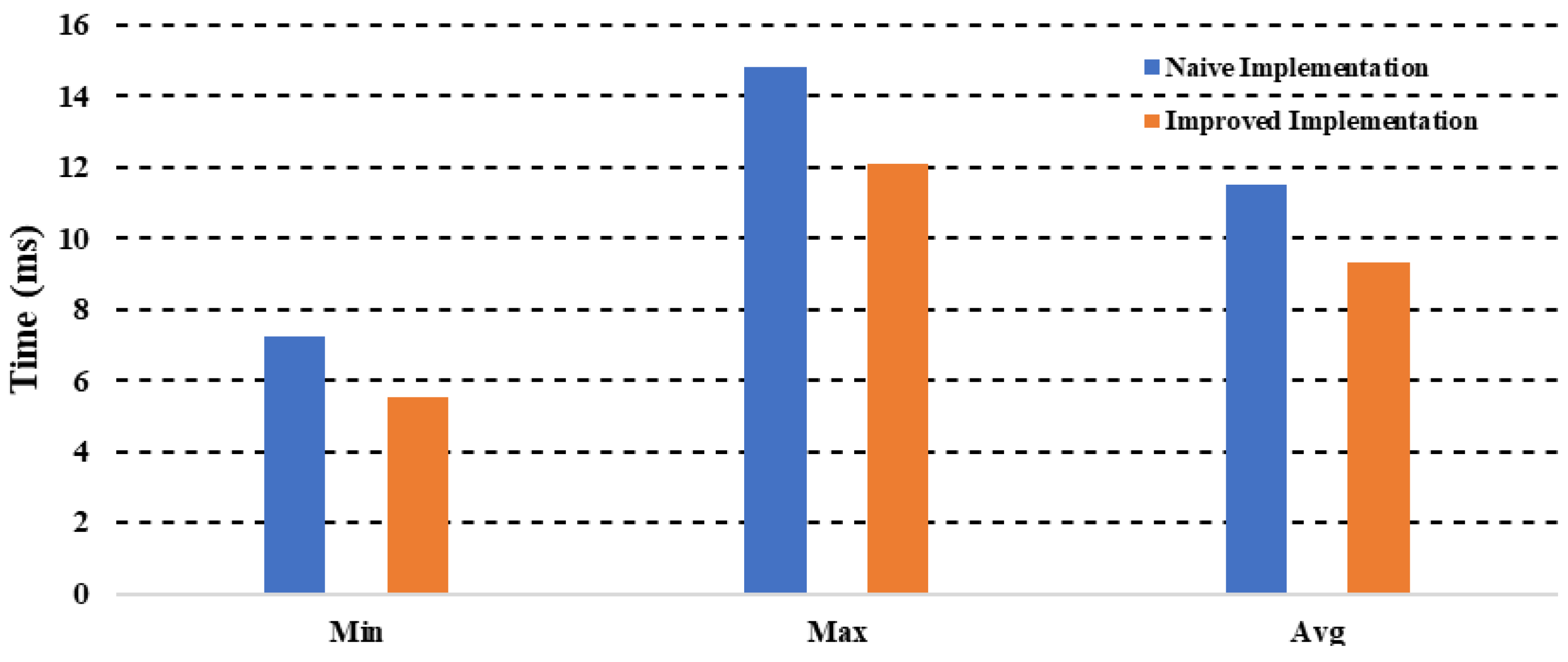
Figure 11 shows a comparison between the naive and improved implementations.
Figure 11 shows that the improved version has a mean processing time of 9.31 ms, compared to the naive version’s mean processing time of 11.5 ms. This improvement allows for processing 107 frames/s compared to 86 frames/s in the naïve implementation.
Consequently, the temporal evaluation has shown that our algorithm can respect the real-time constrain, which is 60 frames/s. In this context, the enhanced implementation has shown an acceleration of ×9 compared to the sequential version, which consumes 90 ms [8]. The time obtained in the sequential version is based on a low resolution compared to our resolution proposed in this paper, which is 5472 × 3648. This shows that the OpenCL-based CPU-FPGA architecture has improved the processing time, even though the resolution is very high.
3.3. Experimental Results
The experimental results are based on calculating the two indices GLI and GRVI in different agricultural fields. The images used in this evaluation have a resolution of 5472 × 3648 pixels for each image collected by the UAV RGB camera used in this study. The temporal evaluation showed that we could process up to 107 images/s with high resolution. This resolution will influence the calculation of the indices. The results obtained were based on the coding of the algorithm with OpenCL in the CPU-FPGA architecture.
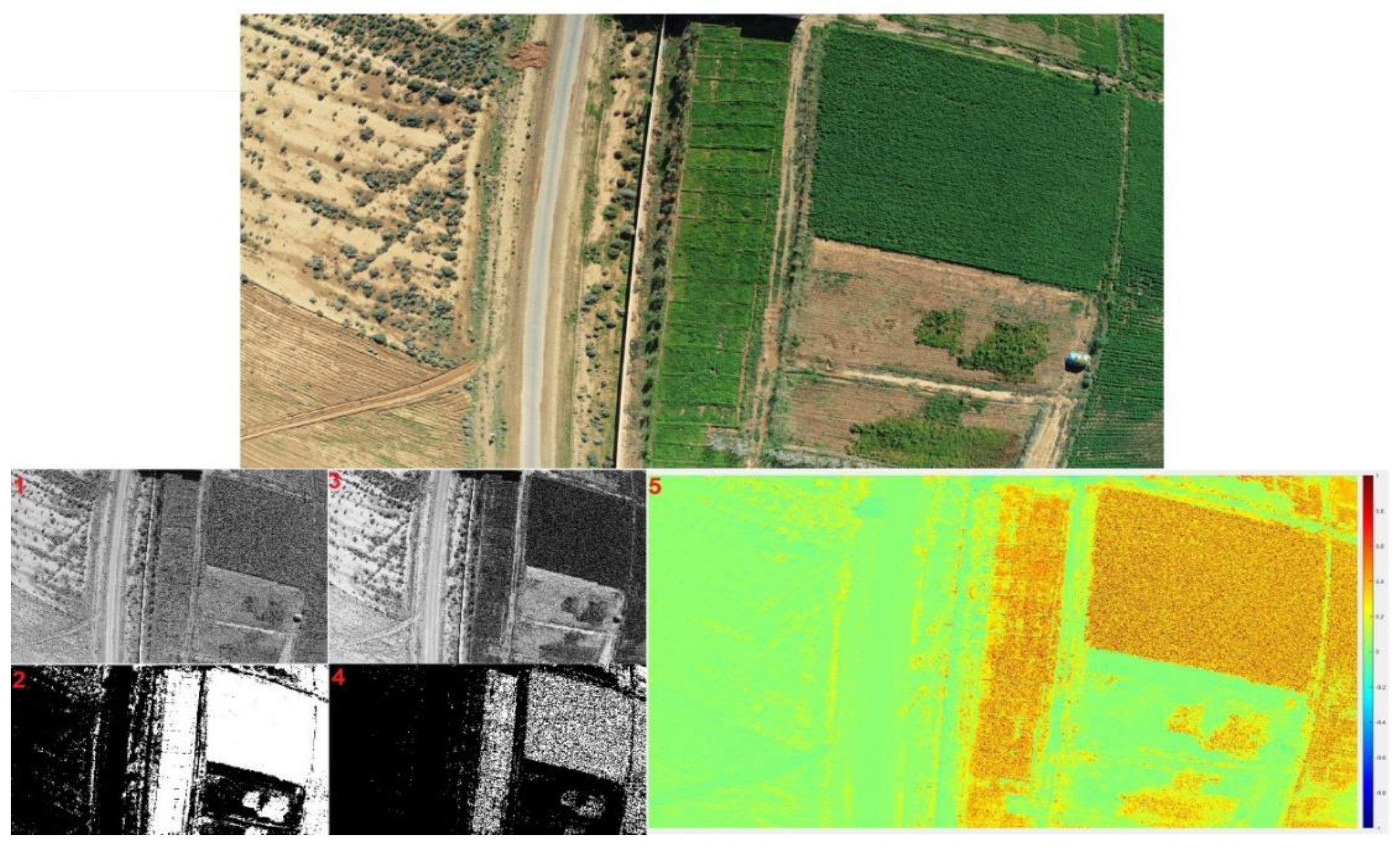
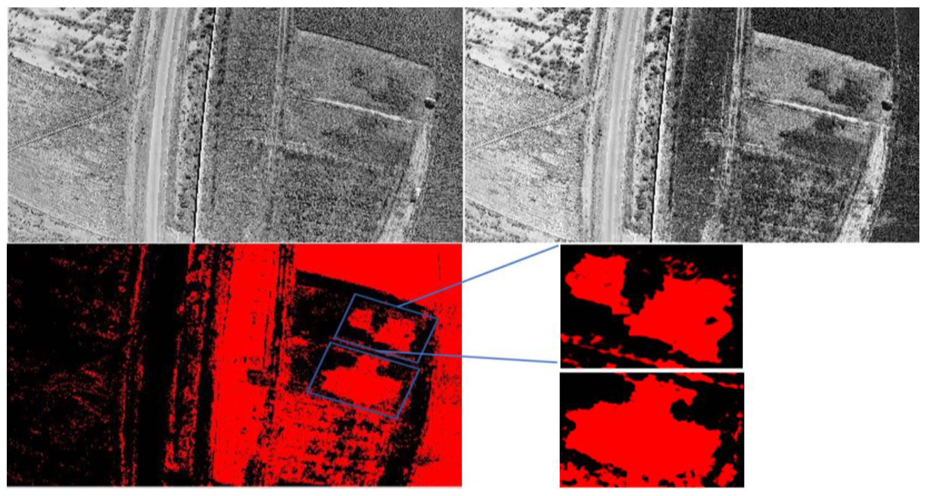
The evaluation of our algorithm was based on two tools, the FPGA SoC embedded platform and the desktop using the Matlab tool. The reason for using Matlab is to validate the results obtained with the FPGA embedded architecture. The algorithm is based on the acquisition of images and then separating these RGB images into different images containing red, green, and blue bands. Then, the prepared images are transferred to the FPGA to process the different indices. The process of calculation is described in detail in [8]. After the calculation of the indices, we binarized images using a thresholding operation in order to be able to interpret the results. Figure 12 shows the results obtained from the evaluation of the second agricultural field.
In Figure 12, the top image shows the three bands that build the RGB image. Images 1 and 3 show the R and G bands after the separation of the bands. In image two, we show the GRVI index based on the thresholding operation. The threshold used in this image is 0.3. In image four, we tried to change the threshold to 0.45 to show the regions with a low index. Figure 13 shows the interpretation of the high index regions.
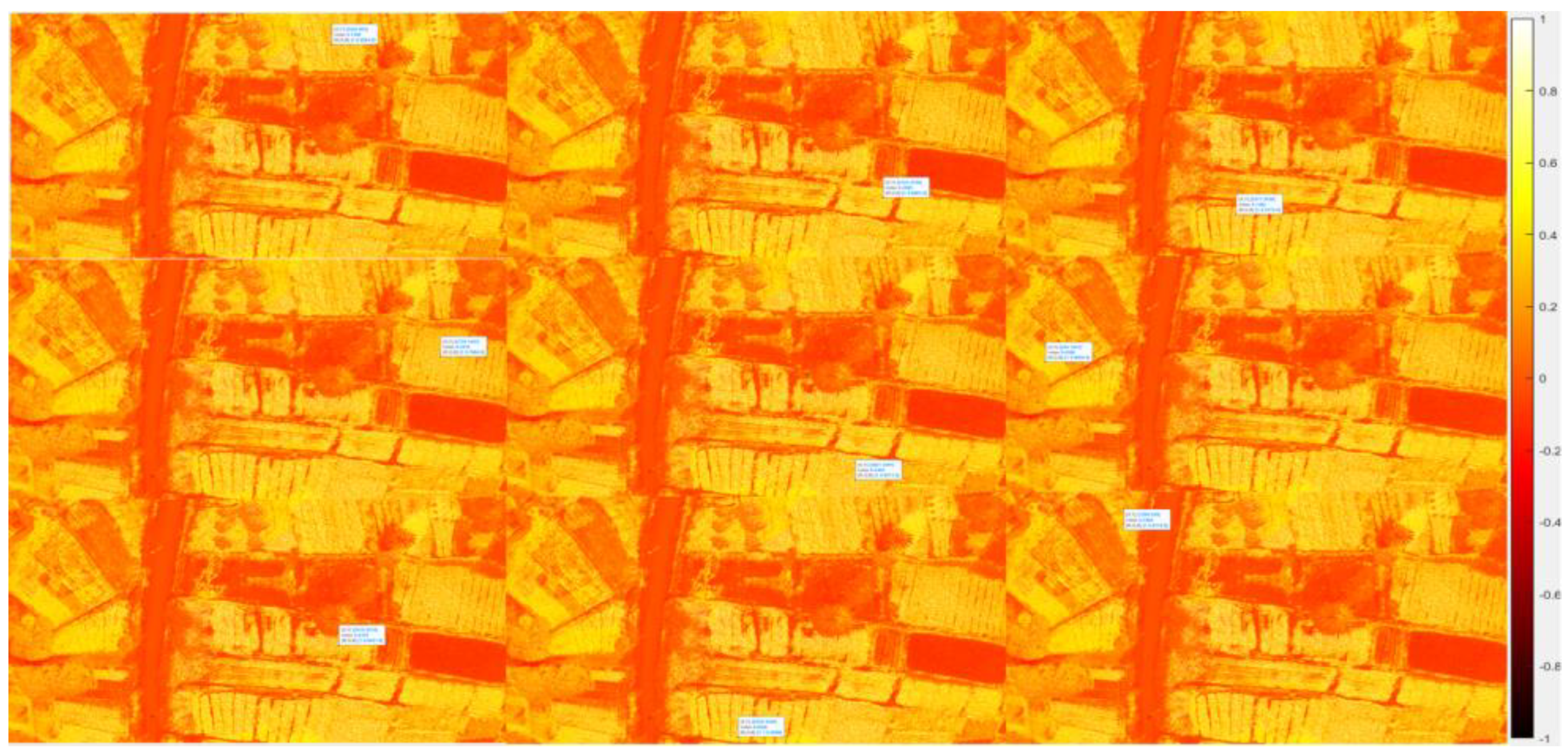
Figure 13 shows the evaluation of the GRVI index. The blue areas indicate regions that have a low index compared to other areas. The interpretation of the results obtained gives the farmer an idea about the agricultural field. The decision is made based on the physiology of each agricultural product. Therefore, the decision and the threshold operation are based on this physiology. Generally, each agricultural product has a specific index threshold. After evaluating the GRVI based on the second agricultural field shown in Figure 3, we evaluated the GLI in the first agricultural field. Figure 13 shows the results obtained.
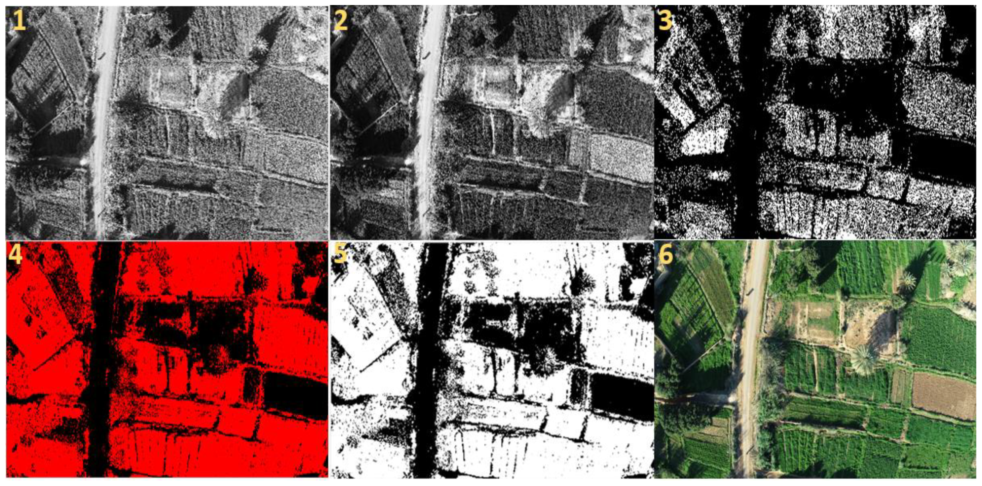
The GLI index is more sensitive than GRVI because it is based on three bands instead of two in the case of GRVI. This fact gives it more visibility than GRVI. On the other hand, the GRVI index is more precise than the GLI index. In our study, we used these two indices because they are the most known and are used for monitoring agricultural fields. In Figure 14, we have evaluated the GLI index of the first agricultural field illustrated in Figure 2. Images 1 and 2 show the red and green bands, respectively, after the separation of the bands. Image 3 shows the results obtained with the FPGA SoC architecture after the thresholding operation.
Similarly, for image 4, we used different thresholds to depict the high value of the index in red. Image 5 shows the binary image obtained with the FPGA SoC platform. Finally, image 6 shows the original image based on the three RGB bands. In the same context and to compare the results, we have also evaluated this index in Matlab to compare the software and hardware implementations. Figure 15 shows the results obtained on Matlab.
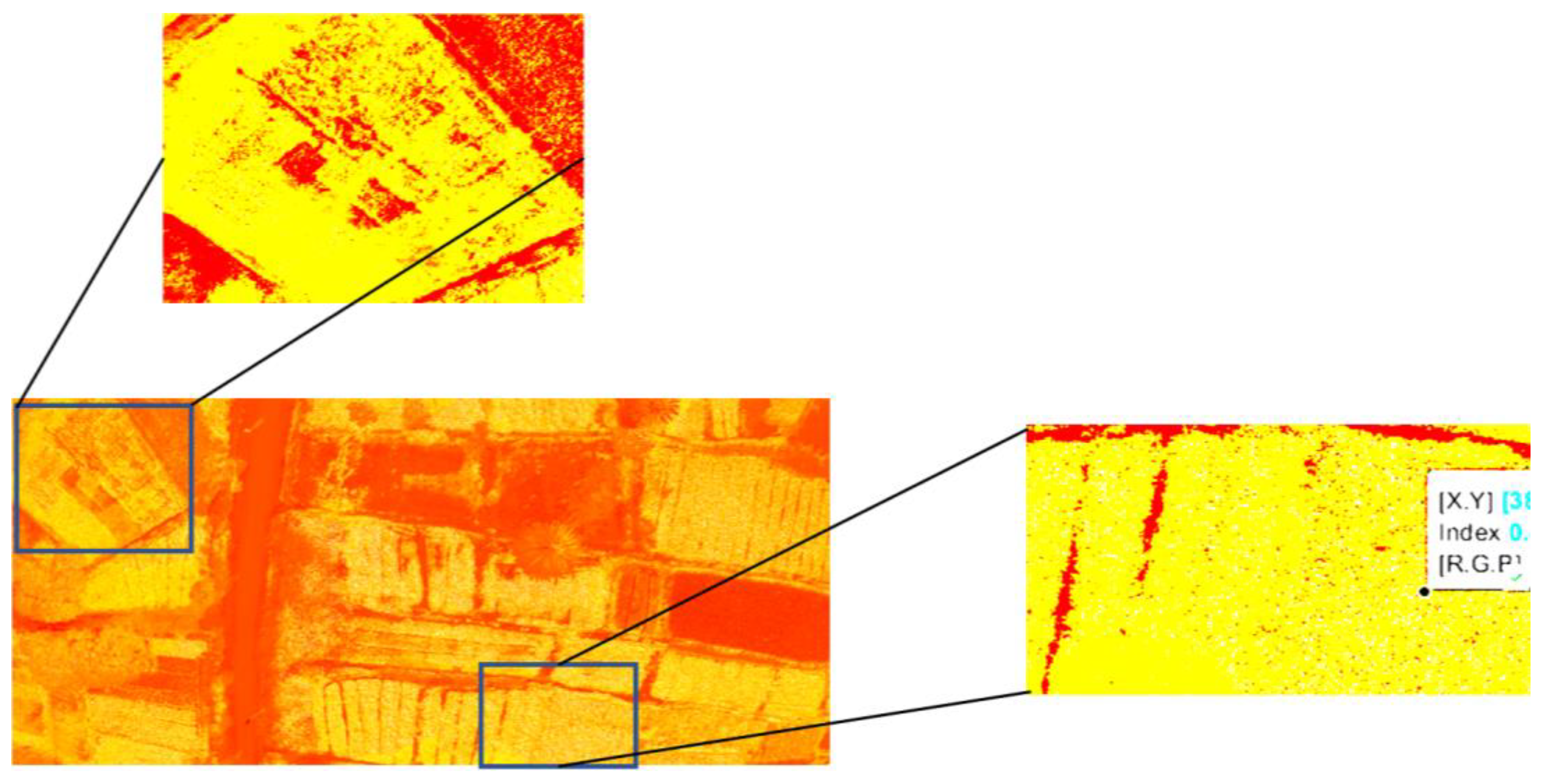
The Matlab evaluation in Figure 14 shows that the FPGA SoC platform gives accurate results based on the Matlab software tool. This shows that this architecture, in addition to its low cost and low consumption, gives robust results. Figure 15 shows the interpretation of the results.
In Figure 16, we have focused on the first region in the blue box at the top left, which gives a matrix of indices values with an average of 0.12. In the blue box at the bottom right, the index evaluation shows a value of 0.6, which offers a high index of GLVI.
3.4. Discussion
The two indices used in this evaluation are known for their high sensitivity to vegetation compared to the other indices. The comparison between the embedded architecture used in this work and the Matlab tool on the desktop shows that the FPGA SoC architecture gave accurate results. In this context, we can find other architectures, such as TX1, TX2, Xavier and other CPU-GPU-type systems. These architectures provide better results, but the problem is the high energy consumption in embedded applications dedicated to precision agriculture. For this reason, the CPU-GPU architecture has a high-power consumption even if we use only a part of the architecture. This leads to high consumption despite the low complexity of the applications. On the other hand, FPGA-based architectures allow the mapping of the algorithm to be implemented. This allows for optimized implementation using the hardware/software co-design approach. This adequation between architecture and algorithm will exploit the lowest amount of resources while maintaining the accuracy of the results.
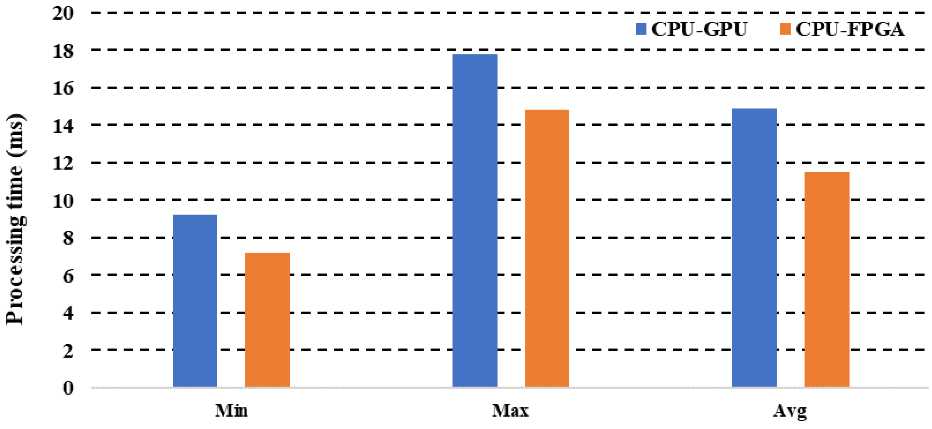
In this study, we have compared XU4 CPU-GPU low-cost architectures with a CPU-FPGA based SoC architecture. The experimental results show that it can take 14.89 ms to process one image with a maximum value of 17.8 ms and a minimum value of 9.2 ms. This processing time was based on the XU4 architecture, which gave a processing rate of 67 frames/s. On the other hand, the processing time using the FPGA SoC architecture was 11.5 ms, which shows that the architecture chosen in this study, along with its low power consumption, reached a processing time lower than the CPU-GPU-based architecture using the same paradigm OpenCL. Figure 17 shows the performances of the two architectures.
4. Conclusions
In this work, we present a CPU-FPGA architecture for index monitoring applications in precision agriculture using the OpenCL paradigm. The results obtained with the SoC FPGA architecture are similar to the results obtained in software implementation based on MATLAB. In addition, the evaluation processing times showed that our algorithm could process 87 frames/s in the naive implementation and 107 frames/s in the improved implementation, with a high resolution of 5472 × 3648 pixels. Compared to the C/C++ implementation, which was based on a resolution of 1280 × 960 pixels, the improvement factor reached 9.6. Thus, our implementation has shown robustness at the processing time level, as well as the number of images processed per second (which exceeds the frame rate of the camera, i.e., 60 frames/s). This responds to the real-time constraints of a monitoring system.
Author Contributions
Conceptualization, A.S.; data curation, A.S.; formal analysis, A.S.; methodology, A.S.; writing—original draft. and A.E.O.; resources, R.L.; supervision, R.L. and A.E.O.; validation, A.E.O.; writing—review & editing, R.L. and A.E.O. All authors have read and agreed to the published version of the manuscript.
Funding
This research received no external funding.
Data Availability Statement
Data sharing not applicable.
Acknowledgments
We owe a debt of gratitude to the National Centre for Scientific and Technical Research of Morocco (CNRST) for their financial support and for their supervision (grant number: 19 UIZ2020).
Conflicts of Interest
The authors declare no conflict of interest.
References
- Shadrin, D.; Menshchikov, A.; Ermilov, D.; Somov, A. Designing Future Precision Agriculture: Detection of Seeds Germination Using Artificial Intelligence on a Low-Power Embedded System. IEEE Sens. J. 2019, 19, 11573–11582. [Google Scholar] [CrossRef]
- Melián, J.M.; Jiménez, A.; Díaz, M.; Morales, A.; Horstrand, P.; Guerra, R.; López, S.; López, J.F. Real-Time Hyperspectral Data Transmission for UAV-Based Acquisition Platforms. Remote Sens. 2021, 13, 850. [Google Scholar] [CrossRef]
- Cortes Torres, C.C.; Yasudo, R.; Amano, H. Body Bias Optimization for Real-Time Systems. J. Low Power Electron. Appl. 2020, 10, 8. [Google Scholar] [CrossRef] [Green Version]
- Spagnolo, F.; Perri, S.; Frustaci, F.; Corsonello, P. Energy-Efficient Architecture for CNNs Inference on Heterogeneous FPGA. J. Low Power Electron. Appl. 2020, 10, 1. [Google Scholar] [CrossRef] [Green Version]
- Latif, R.; Jamad, L.; Saddik, A. Implementation of Hybrid Algorithm for the UAV Images Preprocessing Based on Embedded Heterogeneous System: The Case of Precision Agriculture. In Enabling Machine Learning Applications in Data Science; Hassanien, A.E., Darwish, A., Abd El-Kader, S.M., Alboaneen, D.A., Eds.; Algorithms for Intelligent Systems; Springer: Singapore, 2021. [Google Scholar] [CrossRef]
- McFeeters, S.K. The use of the Normalized Difference Water Index (NDWI) in the delineation of open water features. Int. J. Remote. Sens. 1996, 17, 1425–1432. [Google Scholar] [CrossRef]
- Bastarrika, A.; Alvarado, M.; Artano, K.; Martinez, M.P.; Mesanza, A.; Torre, L.; Ramo, R.; Chuvieco, E. BAMS: A tool for supervised burned area mapping using Landsat data. Remote. Sens. 2014, 6, 12360–12380. [Google Scholar] [CrossRef] [Green Version]
- Saddik, A.; Latif, R.; Elhoseny, M.; El Ouardi, A. Real-time evaluation of different indexes in precision agriculture using a heterogeneous embedded system. Sustain. Comput. Inform. Syst. 2021, 30, 100506. [Google Scholar] [CrossRef]
- Sumesh, K.C.; Ninsawat, S.; Som-ard, J. Integration of RGB-based vegetation index, crop surface model and object-based image analysis approach for sugarcane yield estimation using unmanned aerial vehicle. Comput. Electron. Agric. 2021, 180, 105903. [Google Scholar] [CrossRef]
- Tian, H.; Wang, P.; Tansey, K.; Han, D.; Zhang, J.; Zhang, S.; Li, H. A deep learning framework under attention mechanism for wheat yield estimation using remotely sensed indices in the Guanzhong Plain, PR China. Int. J. Appl. Earth Obs. Geoinf. 2021, 102, 102375. [Google Scholar] [CrossRef]
- Yu, R.; Luo, Y.; Zhou, Q.; Zhang, X.; Wu, D.; Ren, L. A machine learning algorithm to detect pine wilt disease using UAV-based hyperspectral imagery and LiDAR data at the tree level. Int. J. Appl. Earth Obs. Geoinf. 2021, 101, 102363. [Google Scholar] [CrossRef]
- Hunt, E.R., Jr.; Doraiswamy, P.C.; McMurtrey, J.E.; Daughtry, C.S.; Perry, E.M.; Akhmedov, B. A visible band index for remote sensing leaf chlorophyll content at the canopy scale. Int. J. Appl. Earth Obs. Geoinf. 2013, 21, 103–112. [Google Scholar] [CrossRef] [Green Version]
- Li, C.; Li, H.; Li, J.; Lei, Y.; Li, C.; Manevski, K.; Shen, Y. Using NDVI percentiles to monitor real-time crop growth. Comput. Electron. Agric. 2019, 162, 357–363. [Google Scholar] [CrossRef]
- Ren, S.; Guo, B.; Wu, X.; Zhang, L.; Ji, M.; Wang, J. Winter wheat planted area monitoring and yield modeling using MODIS data in the Huang-Huai Hai Plain, China. Comput. Electron. Agric. 2021, 182, 106049. [Google Scholar] [CrossRef]
- Bendig, J.; Yu, K.; Aasen, H.; Bolten, A.; Bennertz, S.; Broscheit, J.; Gnyp, M.L.; Bareth, G. Combining UAV-based plant height from crop surface models, visible, and near infrared vegetation indices for biomass monitoring in barley. Int. J. Appl. Earth Obs. Geoinf. 2015, 39, 79–87. [Google Scholar] [CrossRef]
- Tucker, C.J. Red and photographic infrared linear combinations for monitoring vegetation. Remote. Sens. Environ. 1979, 8, 127–150. [Google Scholar] [CrossRef] [Green Version]
- Bezen, R.; Edan, Y.; Halachmi, I. Computer vision system for measuring individual cow feed intake using RGB-D camera and deep learning algorithms. Comput. Electron. Agric. 2020, 172, 105345. [Google Scholar] [CrossRef]
- Gené-Mola, J.; Vilaplana, V.; Rosell-Polo, J.R.; Morros, J.R.; Ruiz-Hidalgo, J.; Gregorio, E. Multi-modal deep learning for Fuji apple detection using RGB-D cameras and their radiometric capabilities. Comput. Electron. Agric. 2019, 162, 689–698. [Google Scholar] [CrossRef]
- Osroosh, Y.; Khot, L.R.; Peters, R.T. Economical thermal-RGB imaging system for monitoring agricultural crops. Comput. Electron. Agric. 2018, 147, 34–43. [Google Scholar] [CrossRef]
- Shin, J.; Chang, Y.K.; Heung, B.; Nguyen-Quang, T.; Price, G.W.; Al-Mallahi, A. A deep learning approach for RGB image-based powdery mildew disease detection on strawberry leaves. Comput. Electron. Agric. 2021, 183, 106042. [Google Scholar] [CrossRef]
- Isachsen, U.J.; Theoharis, T.; Misimi, E. Fast and accurate GPU-accelerated, high-resolution 3D registration for the robotic 3D reconstruction of compliant food objects. Comput. Electron. Agric. 2021, 180, 105929. [Google Scholar] [CrossRef]
- Moriguchi, K. Acceleration and enhancement of reliability of simulated annealing for optimizing thinning schedule of a forest stand. Comput. Electron. Agric. 2020, 177, 105691. [Google Scholar] [CrossRef]
- Partel, V.; Kakarla, S.C.; Ampatzidis, Y. Development and evaluation of a low-cost and smart technology for precision weed management utilizing artificial intelligence. Comput. Electron. Agric. 2019, 157, 339–350. [Google Scholar] [CrossRef]
- Hussain, N.; Farooque, A.A.; Schumann, A.W.; Abbas, F.; Acharya, B.; McKenzie-Gopsill, A.; Barrett, R.; Afzaal, H.; Zaman, Q.U.; Cheema, M.J. Application of deep learning to detect Lamb’s quarters (Chenopodium album L.) in potato fields of Atlantic Canada. Comput. Electron. Agric. 2021, 182, 106040. [Google Scholar] [CrossRef]
- Song, Z.; Zhou, Z.; Wang, W.; Gao, F.; Fu, L.; Li, R.; Cui, Y. Canopy segmentation and wire reconstruction for kiwifruit robotic harvesting. Comput. Electron. Agric. 2021, 181, 105933. [Google Scholar] [CrossRef]
- Temniranrat, P.; Kiratiratanapruk, K.; Kitvimonrat, A.; Sinthupinyo, W.; Patarapuwadol, S. A system for automatic rice disease detection from rice paddy images serviced via a Chatbot. Comput. Electron. Agric. 2021, 185, 106156. [Google Scholar] [CrossRef]
- Trong, V.H.; Gwang-hyun, Y.; Vu, D.T.; Jin-young, K. Late fusion of multimodal deep neural networks for weeds classification. Comput. Electron. Agric. 2020, 175, 105506. [Google Scholar] [CrossRef]
- Louhaichi, M.; Borman, M.M.; Johnson, D.E. Spatially Located Platform and Aerial Photography for Documentation of Grazing Impacts on Wheat. Geocarto Int. 2001, 16, 65–70. [Google Scholar] [CrossRef]
- Skliarova, I. Accelerating Population Count with a Hardware Co-Processor for MicroBlaze. J. Low Power Electron. Applications. 2021, 11, 20. [Google Scholar] [CrossRef]
Figure 1.
Memory model-based OpenCL architecture.

Figure 2.
Image illustrating area 1.

Figure 3.
Image illustrating area 2.

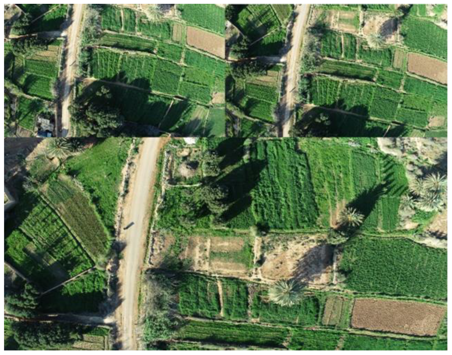
Figure 4.
Images of dataset corresponding to area 1.

Figure 5.
Images of dataset corresponding to area 2.

Figure 6.
Algorithm overview.

Figure 7.
Naive implementation mapping.

Figure 8.
Improved implementation mapping.

Figure 9.
FPGA resources usage after synthesis and placement routing.

Figure 10.
OpenCL time processing.

Figure 11.
Processing time comparison between naive and improved implementations.

Figure 12.
GRVI evaluation based on FPGA SoC architecture compared to MATLAB implementation.

Figure 13.
GRVI interpretation.

Figure 14.
GLI evaluation based on the FPGA SoC platform.

Figure 15.
GLI evaluation based on Matlab.

Figure 16.
GLI interpretation.

Figure 17.
CPU-GPU and CPU-FPGA comparaison.


Table 1.
Recent precision agriculture-based application and tools.
| Reference | Application | Algorithm | Tools |
|---|---|---|---|
| [17] | Cow feed measurement | CNNs Model | RGB-D Camera |
| [18] | Fuji apple detection | R-CNN | RGB-D Camera type Kinect v2 and GPU Nvidia TITAN GTX |
| [19] | Crop monitoring | Image-processing algorithms | Raspberry V3 board and RGB camera |
| [20] | Disease detection | CNNs Model | Workstation |
| [21] | Detection of food objects | ICP algorithm | GTX Nvidia 1080Ti and camera type SR300 RealSense |
| [22] | System of thinning a forest stand | __ | NVIDIA GPU Titan-V |
| [23] | Weed management | __ | GTX NVIDIA GPU 1070 Ti and Jetson TX2 |
| [24] | Lamb’s quarters detection in potato production | DCNN models | GPUs: GTX1080 Ti, GeForce 930MX and GTX1050 |
| [25] | Kiwifruit harvest | __ | Desktop with GPU TITAN XP and RGB camera |
| [26] | Detection of rice disease | YOLOv3 | GPU Tesla V100 |
| [27] | Weeds classification | Multimodal fusion | Tesla K40c NVIDIA |
Table 2.
Evaluation SoC platform specifications.
| FPGA Device | 5CSEMA5F31C6 |
|---|---|
| CPU | ARM CORTEX-A9 |
| Logic Elements | 85 K |
| Embedded Memory | 4450 Kbits |
| SDRAM on FPGA | 32 M × 16 |
| SDRAM on HPS | 2 × 256 M × 16 |
| Communication | USB 2.0 |
| Power | 12 V DC |
Table 3.
Different platform specification.
| Type | Desktop | TX1 | XU4 |
|---|---|---|---|
| Frequency | 2.2 Ghz | 1.9 Ghz | 1.4/2 Ghz |
| Processor | Intel I5 | MPCore | Exynos 5 |
| CPU | Intel | Cortex A57 | Cortex A7/A15 |
| GPU | Intel | Nvidia Maxwell | Mali T628MP6 |
| Energy | 20 W | 15 W | 5 W |
Table 4.
Processing times using different architectures.
| Architecture | Desktop | XU4 | TX1 | |||
|---|---|---|---|---|---|---|
| Executing time (ms) | C/C++ | OpenMP | C/C++ | OpenMP | C/C++ | CUDA |
| 31 | 15 | 91 | 47 | 80 | 0.77 | |
Table 5.
Resource utilization on FPGA.
| Kernel Type. | RAM Blocks | DSPs | FFS | Logic Utilization | Dedicated Logic Registers |
|---|---|---|---|---|---|
| Both Indices | 20.63% | 6% | 12.153% | 25% | 11.53% |
| GNVI | 8.4% | 4% | 5.56% | 10% | 6.12% |
| GLI | 10.2% | 4% | 6.32% | 12.96 | 7.56% |
| Available in the FPGA | 379 | 87 | -- | 32,070 | 77,650 |
Publisher’s Note: MDPI stays neutral with regard to jurisdictional claims in published maps and institutional affiliations. |
© 2021 by the authors. Licensee MDPI, Basel, Switzerland. This article is an open access article distributed under the terms and conditions of the Creative Commons Attribution (CC BY) license (https://creativecommons.org/licenses/by/4.0/).
Share and Cite
MDPI and ACS Style
Saddik, A.; Latif, R.; El Ouardi, A. Low-Power FPGA Architecture Based Monitoring Applications in Precision Agriculture. J. Low Power Electron. Appl. 2021, 11, 39. https://0-doi-org.brum.beds.ac.uk/10.3390/jlpea11040039
AMA Style
Saddik A, Latif R, El Ouardi A. Low-Power FPGA Architecture Based Monitoring Applications in Precision Agriculture. Journal of Low Power Electronics and Applications. 2021; 11(4):39. https://0-doi-org.brum.beds.ac.uk/10.3390/jlpea11040039
Chicago/Turabian StyleSaddik, Amine, Rachid Latif, and Abdelhafid El Ouardi. 2021. "Low-Power FPGA Architecture Based Monitoring Applications in Precision Agriculture" Journal of Low Power Electronics and Applications 11, no. 4: 39. https://0-doi-org.brum.beds.ac.uk/10.3390/jlpea11040039
Note that from the first issue of 2016, this journal uses article numbers instead of page numbers. See further details here.