Article

A Model for the Evaluation of Monostable Molecule Signal Energy in Molecular Field-Coupled Nanocomputing

by
Yuri Ardesi
1,*,
Mariagrazia Graziano
2 and
Gianluca Piccinini
1
1
Department of Electronics and Telecommunications, Politecnico di Torino, 10129 Torino, Italy
2
Department of Applied Science and Technology, Politecnico di Torino, 10129 Torino, Italy
*
Author to whom correspondence should be addressed.
J. Low Power Electron. Appl. 2022, 12(1), 13; https://0-doi-org.brum.beds.ac.uk/10.3390/jlpea12010013
Submission received: 20 January 2022 / Revised: 11 February 2022 / Accepted: 17 February 2022 / Published: 1 March 2022

Abstract

:
Molecular Field-Coupled Nanocomputing (FCN) is a computational paradigm promising high-frequency information elaboration at ambient temperature. This work proposes a model to evaluate the signal energy involved in propagating and elaborating the information. It splits the evaluation into several energy contributions calculated with closed-form expressions without computationally expensive calculation. The essential features of the 1,4-diallylbutane cation are evaluated with Density Functional Theory (DFT) and used in the model to evaluate circuit energy. This model enables understanding the information propagation mechanism in the FCN paradigm based on monostable molecules. We use the model to verify the bistable factor theory, describing the information propagation in molecular FCN based on monostable molecules, analyzed so far only from an electrostatic standpoint. Finally, the model is integrated into the SCERPA tool and used to quantify the information encoding stability and possible memory effects. The obtained results are consistent with state-of-the-art considerations and comparable with DFT calculation.

1. Introduction

Field-Coupled Nanocomputing (FCN) is one of the most attractive technologies proposed to overcome CMOS issues. This work focuses on molecular FCN, where the information is encoded in the charge distribution of molecules that are typically oxidized. Two redox centers allow the positive charge to concentrate on particular points of the oxidized molecule. By aligning two molecules, it is possible to realize square molecular cells where charges order to minimize the electrostatic repulsion, thus creating two stable states that can encode the logic information, see Figure 1a. The definition of logic information relies on the concept of Quantum-dot Cellular Automata (QCA) [1]. FCN can also be realized with several physical interactions; for instance, it is possible to realize FCN computation by using magnets [2,3,4,5,6,7], or atomic silicon or metallic quantum dots [8,9,10].
By aligning different cells, the information propagates in a domino-like way in molecular FCN wires, see Figure 1b. An external electric field, named the clock field [11], generally activated or deactivated regions of the molecular wire, in order to guide the information propagation [12]. Molecular technology promises very high on-chip device density thanks to the natural nanometric size of molecules [13]. It also enables high-frequency operations at ambient temperature and the possibility to use self-assembly techniques. In addition, no current transport is necessary for propagating the binary information, drastically reducing the power dissipation.
This work focuses on the analysis of the energy given to the signal to allow the information encoding and propagation, known in the literature as signal energy [14]. An external electric field, named the clock field [11], typically forces molecules to vary slowly compared to the time constant. In these conditions, the propagation is named adiabatic. In perfectly adiabatic conditions, molecules lie at the ground state configuration, and the signal energy is given back to the clock system when deactivated, rather than dissipated to the environment [14]. The signal energy is vital to understand the information propagation mechanism in the FCN paradigm. Nevertheless, it should not be confused with dissipated energy, which is out of the scope of this work. Within the general QCA paradigm, the dissipated power can be evaluated by studying the interaction between molecule and environment [15,16]. In the molecular FCN, the power dissipation should be also evaluated by considering the dissipation of the clocking electrode system [17].
In this work, we conceive a model for calculating the signal energy of circuits, and we verify it with ab initio calculation. The model computes the signal energy without the need for computationally expensive ab initio calculations. This enables the model to be easily integrated into CAD and simulation tools [18,19], which are gaining more and more importance in the field of FCN design [8,18,20,21,22,23,24], enabling the analysis of signal energy in large circuits with considerable accuracy and without strongly impacting the demand of computational resources, thus favoring the design of future molecular FCN devices. The proposed model is generic and can be applied to any molecule provided it is monostable. Thus, the molecule should be logically neutral at the thermal equilibrium, which means it does provide a polar configuration, eventually encoding logic information. We base our work on the diallylbutane molecule, shown in Figure 1c. This molecule is typically used for modeling purposes [25,26] and was recently announced as a monostable molecule [27]. Moreover, this molecule is reasonably small, facilitating Density Functional Theory (DFT) calculation, and permitting the model validation through ab initio calculation. In fact, the molecular energy of a few diallylbutane molecules can be obtained through DFT calculation in a reasonable computational time.
The proposed model analyses the interaction among molecules by approximating each molecule with a charge distribution, named atomic charges and shown in Figure 1d, obtained by fitting electrostatic potentials generated by the molecule and calculated with ab initio programs. The atomic charges are eventually grouped to obtain the so-called Aggregated Charge [28]. Figure 1e shows the definition of the diallylbutane aggregated charge model. In [29], we demonstrated that the aggregated charge allows evaluating the electrostatic potential generated by the molecule with high precision, without the need for solving integral equations. The aggregated charge allows considering the effective electrostatic behavior of molecules with a low computational cost, fulfilling our aim to provide a model with low computational effort and considerable precision.
We integrate the proposed model into the Self-Consistent Electrostatic Potential Algorithm (SCERPA) [12,30] to demonstrate the possibility to integrate it into Computer-aided Design (CAD) tools easily. Therefore, we use the model to analyze the bistable propagation, and we justify from an energy standpoint, the so-called bistable factors used for determining whether the information can be propagated in circuits [31]. This work provides a theoretical perspective alternative to the standard QCA approach, enabling a deep understanding of the information propagation mechanism in the molecular FCN.

2. Theoretical Methods

This article focuses on the analysis of molecular FCN circuit energy. Each molecule is treated using the MoSQuiTO methodology [28], which models the molecule as an electronic device. The simulation of molecular FCN circuits relies on the Self-Consistent Electrostatic Potential Algorithm (SCERPA) [12,30].

2.1. MoSQuiTo Methodology

The MoSQuiTo methodology consists of a three-step procedure enabling to consider the molecule as an electronic device [29]. DFT calculation evaluates the equilibrium geometry, Figure 1c, and the atomic charges obtained by fitting the electrostatic potential (ESP), also known as ESP charges, (MoSQuiTo step I), Figure 1d. For this work, we make use of the ORCA package [32,33]. The atomic charges are spatially summed to obtain two aggregated charges Q 1 and Q 2 which model the molecule electrostatic behaviour (MoSQuiTo step I), Figure 1e. The aggregated charges depend on electric fields that might be generated by electrodes for implementing possible drivers [34], Figure 2a. The electric field is described by the so-called input voltage ( V i n ) evaluated as:
V i n = λ E i n dl
where E i n is the electric field generated by the two electrodes, whereas λ is a generic path connecting the position of the two diallylbutane dots (formally positioned on the two carbon atoms enlarged and colored in blue in Figure 2a). The link between the aggregated charge and the input voltage is known as Vin-Aggregated Charge Transcharacteristics (VACT) [29].
In addition to external electrodes, the electric field might also be generated by other molecules, permitting the information propagation, as schematized in Figure 2b. In this case, a driver molecule generates an electric field (denoted as E i n ) impacting the Molecule Under Test (MUT). Again, it is possible to measure an input voltage V i n by integrating the field E i n . The MUT reacts with a charge displacement that creates a second electric field influencing other molecules. A possible “fictitious molecule”, positioned at the same driver-MUT distance receives the effect of E o u t . It is possible to evaluate the so-called output voltage of the MUT by integrating the field E o u t on a path connecting the two dots of the fictitious molecule, according to Equation (1). Finally, the electrostatic model permits the analysis of molecular FCN circuits by considering the effective molecule behavior without complex ab initio calculation. This methodology allows the SCERPA tool [12,30] to iteratively evaluate the field generated by molecules to obtain the charge distribution of the molecular circuit, eventually deriving the cross-implications between molecular physics and circuit behaviour [35].

2.2. Bistable Factor

The propagation of the information in a molecular wire based on monostable molecules can be evanescent or bistable. The propagation is evanescent when only a few molecules propagate the information, whereas it is named bistable when all the molecules alternate the polarization (i.e., the displacement of the molecule charge distribution). The polarization can be described by the so-called Bistable Factor, which is fully described in [27]. We here report the necessary basics to understand this work.
In bistable propagation, the polarization of adjacent molecules alternates; if the polarization is correlated to the input voltage, this implies two adjacent molecules are subjected to opposite input voltages, named V S A T . Considering the trivial case of two molecules, the same input voltage also implies the same output voltage. That means, for a single molecule, V o u t / V i n = 1 . More in general, the bistable propagation is possible if, for a small input voltage, the molecule reacts with an output voltage that tends to increase the input voltage for the adjacent molecule towards the V o u t / V i n = 1 condition. Formally, this is described by the bistable factor B F 0 :
B F 0 ( d , L , α ) = lim V i n 0 V o u t V i n
where d is the intermolecular distance, L is the width of the molecule (here labeled L instead of w as in the original manuscript, to avoid confusion with energy quantities), and α is the so-called polarizability. The polarizability is the tendency of a molecule to create a dipole moment when subjected to an electric field.
In a wire composed of N molecules, the input voltage of a single molecule depends on the output voltage of all the molecules in the circuit. Thus, the so-called centered bistable factor ( B F N c ) is generally defined by considering a molecule in the center of two N-molecule wires and by evaluating the input voltage considering the effect of all the molecules of the wire, as depicted by Figure 2c.
B F N c = 2 n = 1 N ( 1 ) n + 1 B F 0 n d , L , α
The bistable factor will be used in Section 4.4 to demonstrate its effectiveness and the characteristics of the bistable propagation from an energy standpoint. Indeed, according to the theory [31], B F N c describes the possibility to have bistable propagation using monostable molecules. The information propagation is possible if a small variation of the input voltage implies a larger variation of the output voltage, which means the bistable factor exceeds 1.

3. Energy Modelling

In this section, we introduce the proposed energy model for evaluating signal energy in the molecular FCN paradigm based on monostable molecules. Section 3.1 describes the reference system used to model the molecular circuit and the main contributions taking part in the evaluation of the signal energy, which will be named internal and interaction energies. Then, Section 3.2 and Section 3.3 describes the internal energies related to the conformation of the molecule and the polarization, respectively, whereas Section 3.5 and Section 3.4 describe the interaction energies related to possible external electric fields and surrounding molecules, respectively. Finally, Section 3.6 derives the complete model for the evaluation of the molecular FCN signal energy circuit.

3.1. Model Definition

Quantum chemistry rigorously evaluates the energy of molecules by solving the Schröedinger equation. The approach is exact yet computationally challenging when dealing with many-molecule systems.
In this work, we provide an efficient model to evaluate the total energy W t o t of a molecular FCN circuit comprising N molecules. The proposed model uses physical chemistry and electrostatic equations to reduce the computational effort in evaluating the Schroedinger equation and permitting the eventual integration into CAD tools. The quantum nature of the molecular system is wholly embedded in the derivation of the molecular characteristics, performed through ab initio calculation. We assume the Born–Oppenheimer approximation: The electrostatic interactions are considered non-geometry influencing. Nuclei are assumed fixed in the space. We split the energy problem into two main contributions, in turn, divided into two subcomponents. Thereinafter, we will model the energy of single molecules or systems composed of a group of molecules. We denote with lowercase w a single energy contribution (e.g., w 0 is the conformation energy of a single molecule) whereas uppercase W denotes the energy of a group of molecules (e.g., W 0 is the conformation energy of a group of non-interacting molecules). Superscripts associate the single energy contribution to a precise molecule (e.g., w 0 ( i ) is the conformation energy of a generic molecule i). In the following paragraphs, we discuss and model the four subcomponents.
Figure 3 shows a system of two diallylbutane molecules exposed to the influence of an electric field (E). The system internal energy W m depends on the internal energy of each molecule ( w m ( 1 ) and w m ( 2 ) ), double-underlined red quantities in Figure 3). It is composed of the conformation energy of the molecules ( w 0 ), which is a property of the single isolated molecule, and the dipole induction energy ( w μ ), gained by each molecule when exposed to an external electric field due to polarization.
The interaction energy W i n t depends on the electrostatic interaction between molecules ( w m m ( 1 , 2 ) ), and between molecules and external electric fields ( w E ( 1 ) , w E ( 2 ) ) (blue single-underlined quantities in Figure 3). With reference to Figure 3, the two molecules are oxidized; therefore, they retain a positive charge on the two molecules. For this reason, the two molecules create radial electric fields which are responsible for the intermolecular interaction, thus w m m ( 1 , 2 ) , that generate opposite dipoles on the two molecules [35]. In addition, the molecules also experience polarization induced by the electric field (E), which makes the two dipoles not perfectly opposite but slightly rotated towards the direction of the external electric field (E). Finally, in the case depicted in the figure, we should expect Mol 1 to maintain the charge in the center of the molecule, since the electric field (E) and the electric field generated by Mol 2 compensate each other, whereas we expect Mol 2 to polarize due to the consistent alignment between the electric field (E) and the radial electric field generated by Mol 1 on Mol 2.

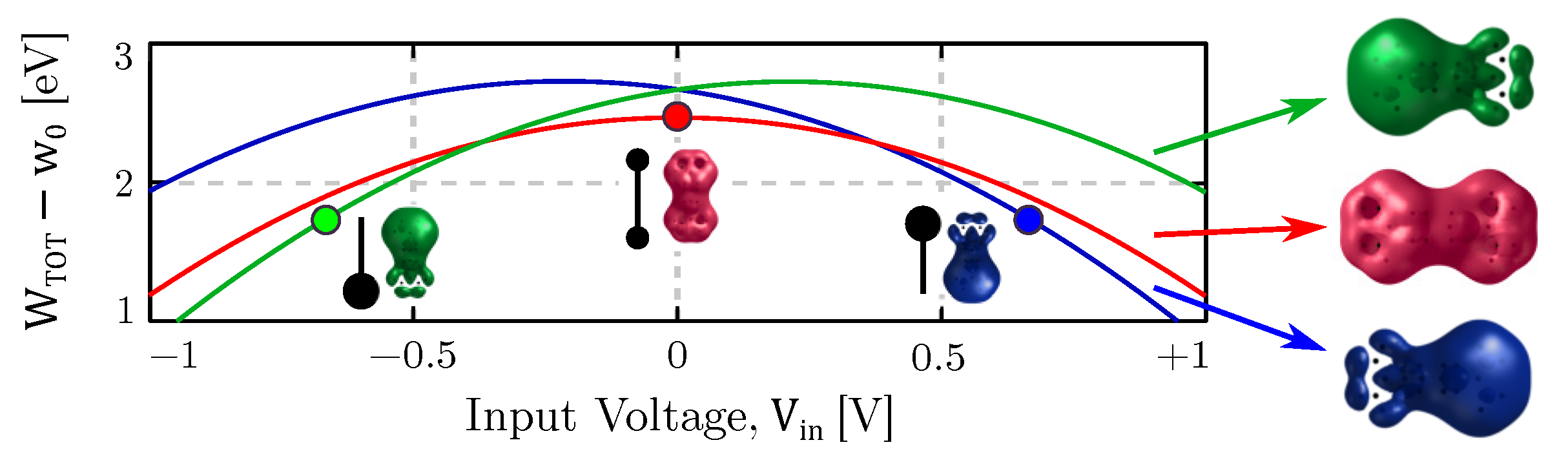
3.2. Internal Energy: The Conformation Energy

We employ the Density Functional Theory (DFT) to compute the energy of the single molecule w 0 numerically. In general, it is possible to evaluate w 0 by solving the molecular Schröedinger equation [36]. Naming Ψ m o l and H ^ m o l the molecule wavefunction and the molecular hamiltonian operator respectively:
w 0 = Ψ m o l | H ^ m o l | Ψ m o l Ψ m o l | Ψ m o l
Dealing with monostable molecules, w 0 is the energy of the equilibrum configuration, thus it matches the molecule minimum energy configuration. Any perturbation applied to the molecule increases the internal energy w m .
We evaluate the total conformation energy W 0 as the energy of a system composed of N non-interacting molecules (ideally, the distance among molecules is consider infinite). Indeed, at the current state, molecular FCN circuits are typically conceived as molecular monolayers constituted by a single molecular species [11,37]. As a consequence, the system conformation energy is:
W 0 = i = 1 N w 0 ( i ) = N w 0
The evaluation of the conformation energy is very time-expensive but generally not necessary. The conformation energy is constant and supposed to be available in the literature if the circuit relies on well-known molecules, or evaluated the first time only. In the next paragraphs, we evaluate the energy contributions related to the interaction among molecules.

3.3. Internal Energy: The Polarization Energy

When an electric field E generated by electrodes or other molecules influences a molecule, the electron cloud of the latter molecule reshapes to minimize the electrostatic energy resulting in the interaction with the external field, here named w E . As a consequence of the electron cloud reshape, the charge of the molecule is not uniformly distributed, and the isopotential surface is deformed [38]. The isopotential surface enlarges where a positive charge is present. Figure 4a shows the isopotential surface of the molecule evaluated before the molecule polarises in the exact moment the electric field is applied (situation denoted as [A]). The electric field induces a displacement of the molecule charge center in the direction of the field, inducing a non-zero dipole moment μ , and leading the molecule to the configuration denoted as [B], see Figure 4b. Since the considered molecule is monostable, the molecular energy increases by a quantity w μ , so that w m = w 0 + w μ > w 0 , see Figure 4c. Notice this method is different to typical energy approaches used to analyze the general QCA paradigm, used for instance in QCADesigner [16]. Indeed, the general QCA paradigm based on bi-stable molecules usually employs the Two-State Approximation (TSA) to model molecular physics. In the TSA case, the energy minima are placed on the two polarized states rather than in the non-polarized one. Therefore, the monostable molecule considered in this work should be studied with a different theory, which correctly positions the molecule energy minimum in the non-polarized state, implying the molecule to polarize only if an external electric field is present.
If the applied field is small, the induced dipole moment μ can be expressed in the so-called linear dipole approximation [39] as:
μ = α E
where α is the molecule polarizability and describes the linear response of the molecule to external electric fields. It is essential to highlight the need for monostability since this is a requirement of the molecule to be used with the proposed model. The proposed model requires the molecule to be monostable. As an example, the used diallylbutane is recognized as a monostable molecule intended to provide calculation capabilities [27]. Bistable molecules can be eventually studied with the TSA [38]. For the sake of completeness, we discuss in Appendix A the energy analysis of a bistable molecule analyzed with the TSA. The energy variation associated with the polarization of a monostable molecule is well-known in the literature [39]:
Δ u = 1 2 α | E | 2
The energy Δ u represents the work performed by the molecule during the polarization process. The potential energy is evaluated as:
w μ = Δ u = 1 2 α | E | 2
The polarizability mechanism of a molecule can be modeled as a charged harmonic oscillator under the influence of an external electric field [40]. For this work, we employ the equivalent mechanical system depicted in Figure 4. We can evaluate the corresponding dipole moment of the mechanical system μ s as:
μ s = q x
When the charge is in the equilibrium position, see Figure 4d, the mechanical system shows null dipole moment, equivalently to the configuration [A] of the molecular system. The external electric field ( E ) accelerates the charge (q) by acting with an electrostatic force F e l = q E . The force moves the charge in a second position x 0 = q | E | / 2 k , see Figure 4e, which represents the displacement of the molecule electron cloud in configuration [B]. The two mechanical springs, characterized by stiffness k, model the restoring force F r e attempting to bring the molecule at the equilibrium. The dipole moment of the mechanical system in configuration [B] is evaluated according to Equation (6):
μ s | x 0 = q 2 2 k | E |
A linear relation between the electric field and the dipole moment holds at the mechanical equilibrium. This situation, shown in Figure 4e is equivalent to the case of a polarized molecule, shown in Figure 4b.
Therefore, by comparing Equation (5) with Equation (7), we relate the stifness parameter of the mechanical system to the molecular polarizability:
k = q 2 2 α
The energy of the mechanical system in the equilibrium position ( x 0 ), taking into account that x 0 = q | E | / 2 k :
w s | x 0 = k x 0 2 = q 2 4 k | E | 2
Out of the equilibrium condition (i.e., μ α E ) the position of the charge x in the mechanical system can be linked to the dipole moment according to Equation (6). Therefore the energy of the mechanical system can be evaluated as:
w s = k x 2 = q 2 2 α | μ | q 2 = μ 2 2 α = w μ
This equation models the energy increase of the molecule when an external electric field induces a dipole moment. DFT computation allows evaluating the polarizability α of single molecules.
Notice that external electric fields might apply in different directions. Fields on the switching direction realize drivers, whereas orthogonal electric fields implement the so-called clocking mechanism [11]. The polarizability may be different on the directions (anisotropy) and can be described with a 3 × 3 matrix:
μ μ 0 = α E = α x x α x y α x z α y x α y y α y z α z x α z y α z z E
In general, the term { α i j } of Equation (11) represents the attitude of the molecule to create a dipole moment along the direction i as a response of a field along the direction j. In many cases, if the coordinates are accurately chosen, the terms { α i j } (with i j ) can be neglected. In this work, we approximate the polarizability α as a diagonal matrix, implicitly stating that any electric field induces a dipole along the same direction and neglecting molecule anisotropy. More in general, an electric field produces a variation of the molecule. Indeed, the molecule might be polar, showing a non-zero dipole moment at the equilibrium μ 0 . The general expression of the induced dipole moment can be evaluated as the difference between the molecule dipole moment and the equilibrium dipole moment:
μ μ 0 = α x x 0 0 0 α y y 0 0 0 α z z E
Therefore, the general espression for the energy contribution is finally evaluated by expanding Equation (10) to the three polarizability components:
w μ = ( μ x μ 0 , x ) 2 2 α x x + ( μ y μ 0 , y ) 2 2 α y y + ( μ z μ 0 , z ) 2 2 α z z = ( Δ μ x ) 2 2 α x x + ( Δ μ y ) 2 2 α y y + ( Δ μ z ) 2 2 α z z

3.4. The Interaction Energy: Intermolecular Energy

To evaluate the field generated by each molecule, we approximate the single M-atom molecule as a distribution of M atom-centered charges evaluated by fitting the electrostatic potential according to the Merz-Singh-Kollman approach [41]. Considering two generic molecules (denoted as m i and m j ), modeled with the charges { q α } and { q β } respectively, the intermolecular interaction energy can be evaluated following the model reported in [35] as:
w m m ( i , j ) = 1 4 π ε 0 α m i β m j q α q β | r α r β |
where r α and r β represent the position of the atomic charges. Therefore, the total intermolecular interaction in the N-molecule circuit is:
W m m = 1 2 i , j [ 1 , N ] , j i w m m ( i , j )
The factor 1 / 2 avoids counting two times a single interaction, since w m m ( i , j ) = w m m ( j , i ) .

3.5. The Interaction Energy: Electric Field Energy

As already mentioned, electric fields deform the molecular charge distribution, inducing a dipole moment μ . The energy associated with the interaction between the molecule, described by a set of charges { Q α } , and the applied electric field E is evaluated as:
w E = μ · E
The dipole μ can be linked, with very good precision, to the value of the atomic charges [29] as:
μ = α q α · r α
where the vector r α = ( x α , y α , z α ) represents the position of atomic charge q α of a generic molecule.

3.6. Final Expression

To sum up, given a circuit composed by N molecules, denoted as { m 1 , , m N } , with each molecule subjected to a possible external electric field E i generated by external electrodes, the final energy can be evaluated as:
W T O T = N w 0 + i [ 1 , N ] ( Δ μ x , i ) 2 2 α x x + ( Δ μ y , i ) 2 2 α y y + ( Δ μ z , i ) 2 2 α z z + + 1 8 π ε 0 i , j [ 1 , N ] , j i α m i β m j q α q β | r α r β | i [ 1 , N ] μ i · E i

4. Results

This section begins by analyzing the energy of a diallylbutane molecule using DFT to derive the basic properties of the equilibrium (the conformation energy w 0 and the equilibrium dipole moment μ 0 ), Section 4.1, and under the influence of electric fields (the polarizability matrix α ), Section 4.2. The proposed energy model is then used to evaluate the energy of molecules under the effect of electric fields, and in molecular systems. The results are compared to DFT calculations to validate the proposed model, Section 4.2 and Section 4.3. Secondly, the model is used to study the bistability characteristics of the information propagation. We demonstrate from an energy standpoint the validity of the bistable factor theory in analyzing monostable molecules, Section 4.4. Finally, we integrate the energy model into the SCERPA tool. We demonstrate the possibility of using the model in CAD tools and demonstrate the capability of molecular FCN wires to retain information, Section 4.5

4.1. Equilibrium Analysis

The geometry of the oxidized diallylbutane is optimized by using the Kohn-Sham scheme with the Becke-Johnson damping scheme (D3BJ) [42,43]. Authors in [27] compared different ab initio techniques and reported CAM-B3LYP as correct DFT functional to correctly consider the symmetry of the molecule, making it possible considering the diallylbutane as a monostable molecule. The authors verified the monostability of the molecule using CAM-B3LYP/6-31G*. In this work, we make use of the CAM-B3LYP, and we improve the precision of the calculation by using the basis set def2-TZVPP [44]. The obtained equilibrium geometry is reported in Figure 5a. The conformation energy of the molecule is evaluated through DFT: w 0 = −390.206 Eh (−10,618 eV).
Figure 5b shows the iso-potential surface of the molecule, evaluated at 3.4 V. In the absence of applied electric fields, asymmetric iso-potential surface denotes the presence of a negligible dipole moment at the equilibrium μ 0 = ( 0.0023 , 0.000025 , 0.000076 ) D (1 D is 3.336 × 10 30 C·m). The obtained small dipole moment confirms the non-polar nature of the diallylbutane cation, confirming the result reported in [27] obtained with CAM-B3LYP/6-31G*. The geometry optimization of the molecule required 1 h 25 min and 14 s, whereas the single-point calculation required 13 min and 26 s. All the calculations were performed on four cores, Xeon Gold 6134.

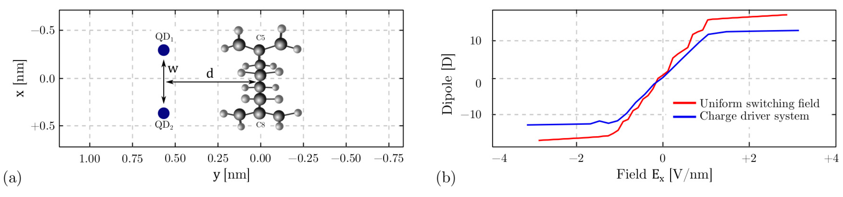
4.2. Field-Induced Polarization of the Diallylbutane

To obtain the polarizability, we study the response of the molecule to electric fields using two methods. At first, the polarizability is obtained with DFT calculation using the numeric differentiation of dipole procedure implemented in the ORCA package. The molecule is analyzed by stimulating the molecule with electric fields on the order of 0.001 a.u. (≈0.5 V/nm). The resulting polarizability matrix is:
α = 2837.5818 0.1008 4.5466 0.1008 129.7067 0.0016 4.5466 0.0016 79.9294 a . u .
The largest matrix elements belongs to the matrix diagonal (A first polarizability analysis permits the evaluation of the polarizability matrix eigenvectors. Hence, the coordinates of the molecule geometry are changed to maximize the final polarizability matrix diagonal elements.). The polarizability can be approximated with Equation (12) by assuming: α x x = 2837.58 a.u., α y y = 129.71 a.u., and α z z = 79.93 a.u. (For the polarizability, 1 a.u. is 1.649 × 10 41 C·m 2 /V).
The second method analyzes the molecule under the influence of electric fields by evaluating the dipole moment and linearly fitting it on the electric field value. The ORCA package allows inserting static fields through the definition of background charges. The molecule is positioned between two point charges with value Q and Q and distance d = 10 nm, see Figure 6a. In this system, the electric field can be computed as E x = 2 Q / ( π ε 0 d 2 ) .
The molecule is studied by gradually shifting the background charge Q in the range ±25 a.u., which corresponds to a ±3 V/nm electric field. We collect the dipole moment μ and the energy W T O T resulting from each DFT computation.
Figure 6b shows the dipole moment obtained with DFT analysis. The dipole moment increases consistently with the electric field. By fitting the dipole moment in the central region, following equation (5), we obtain the polarizability α x x = 2889.95 a.u. This value is consistent with the one obtained through direct DFT computation, confirming the previous method validity. For the next analyses, we decide, as an example, to consider α x x = 2837.58 a.u. (i.e., the polarizability obtained with the ORCA procedure).
Figure 7a, dashed red line, shows the total energy obtained by the DFT calculation. Each point denotes the configuration of a single simulation obtained with a precise electric field (reported on the x-axis).
We analyze each point with the proposed energy model by considering the four previously discussed contributions. The equilibrium energy w 0 is, by definition, constant and equal to the value obtained in Section 4.1. Figure 7b shows the electric field energy w E , evaluated using Equation (16). The electric field induces a dipole following the electric field direction, decreasing the energy μ x E x .
Figure 7c shows the molecule polarization energy w μ , obtained with Equation (13), introduced by the interaction between the electric field and the molecule and which allow the molecule to reshape its charge distribution: The larger the electric field, the larger the charge distribution modification and the consequent energy variation. Since there is only one molecule, the intermolecular interaction is not present. Figure 7c also shows with dashed red line the energy obtained with (9) representing the ideal internal energy obtained in the case of a linear molecule behavior. In the considered case, the molecule is linear for a small electric field: The dipole moment saturates for large electric field values. The use of the proposed model, whose polarization energy is evaluated with (13), allows better considering the non-linearity of the molecule, eventually providing a more accurate description of the polarization energy. The obtained parabolic trend confirms the monostable nature of the diallylbutane cation, confirming the result reported in [27] obtained with CAM-B3LYP/6-31G*. Figure 7a, solid black line, compares the sum of the three energy contributions ( w 0 + w E + w μ ) with the total energy obtained with DFT calculation. The two curves almost overlap, validating the method developed in this work. Figure 7d reports the absolute error between the two curves, which appear lower than 0.02 eV (lower than 2 × 10 4 % on the total energy, about 2% relative error if considering only the energy variation).

4.3. Intermolecular Interaction

In this section, we evaluate the interaction between molecules. We exploit DFT calculation to evaluate the atomic charges and the total energy of two oxidized diallylbutane molecules positioned at different distances (d). To consider the oxidation state of the two molecules, the total charge of the molecular system is 2 a.u. (For the charge, 1. a.u. is 1.6 × 10 16 C), no background static field is present in the analysis.
Figure 8a, black line, reports the energy calculated by the DFT analysis deprived by the equilibrium energy of the two molecules ( W 0 = 2 w 0 ). The electrostatic intermolecular interaction strength decreases with the intermolecular distance, justifying the obtained decreasing energy trend.
For all the simulations, we evaluate the intermolecular interaction energy W m m using Equation (15) by using the atomic charges obtained from DFT. Figure 8a, blue line, compares the obtained interaction energy W m m with the ab initio values. Figure 8b, blue line, reports the error between the DFT result and the model prediction. For typical intermolecular distances (i.e., comparable with molecular width), the error is on the order of 0.01%.
By decreasing the intermolecular distance (d), the electrostatic interaction increases, favoring the polarization of molecules. The polarization of each molecule implies a variation of the dipole induction energy w μ . The contribution w μ is evaluated using Equation (13) and added to the interaction energy, see Figure 8a, red line. The error is on the order of 0.001%, see Figure 8b, dashed red line.
For very low intermolecular distances, the distance between atoms of the single molecule is comparable with distances among atoms of different molecules. The two molecules cannot be considered two independent elements, and the proposed model is out of the validity scope, justifying the increasing error between DFT and model results.
Figure 8c reports the interaction energy evaluated with different atomic charge approximations in the range 0.6–1 nm. Figure 8d reports the associated relative error evaluated with respect to the DFT calculation. In particular, we consider the charges obtained from the fitting of the electrostatic potential (ESP charges), the Mulliken charge and the Lowdin charges. As expected, the ESP charges provide the lowest error in describing the electrostatic behaviour of the molecule, lower than 0.1 eV, thus motivating the use of this charge approximation for determining the interaction energy.

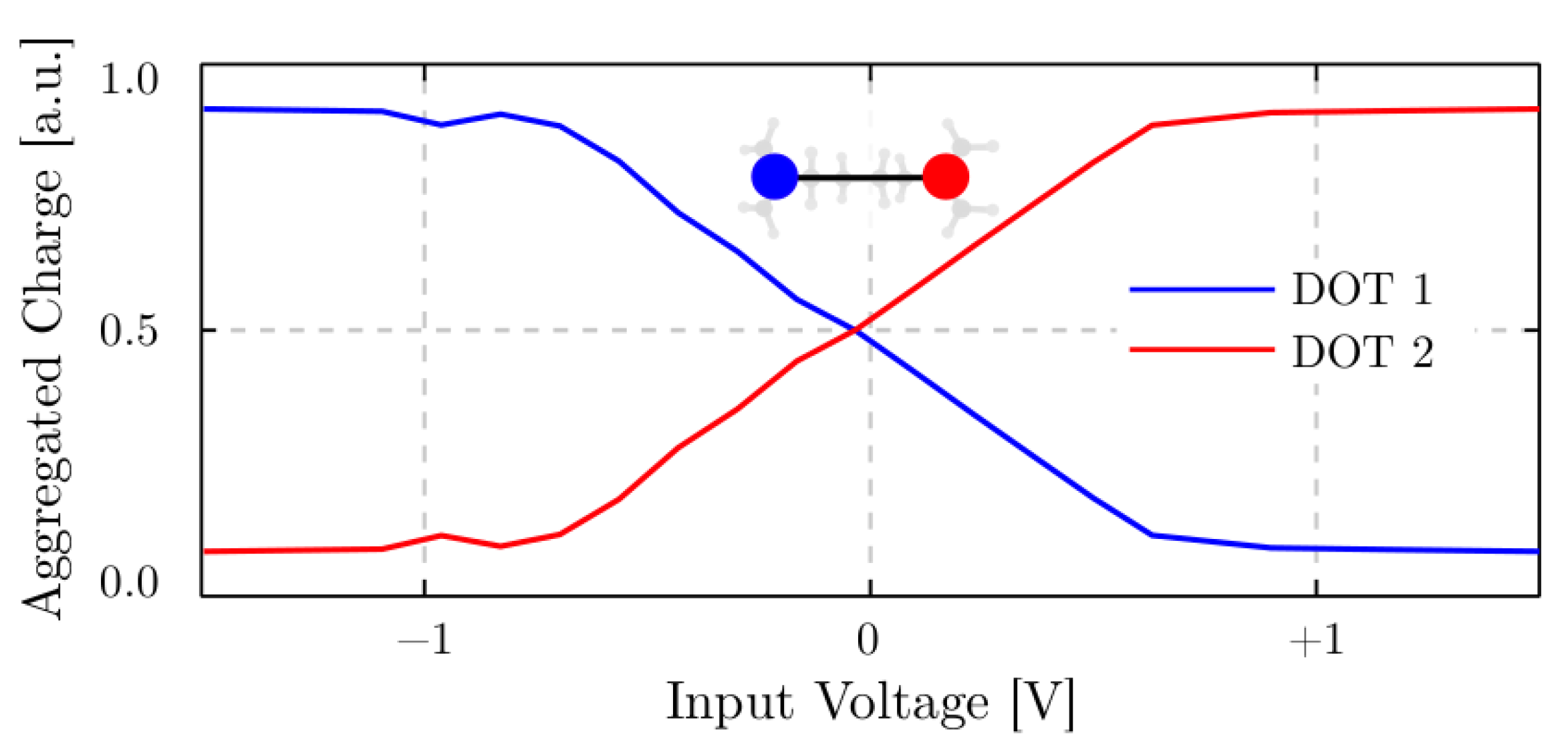
4.3.1. The Driver Response

In this paragraph, we study the response of the single molecule (Molecule Under Test, MUT) to the effects of a driver molecule positioned as depicted in Figure 9a. Two charges Q D 1 and Q D 2 , aligned with atoms C5 and C8, emulate the presence of a molecule whose polarization is forced by external electrodes. The distance between the two charges (L) equals the intermolecular distance (d). This schematic is commonly used to characterise the driver-molecule interaction. The value of the charges is gradually varied to study the driver-molecule interaction. The two charges generate a switching electric field on the molecule under test describable by the so-called input voltage V i n [29].
V i n = 1 4 π ε 0 d 2 2 2 Q D 1 Q D 2
Figure 9b, solid line, reports the dipole moment obtained for different input voltages (i.e., different driver charges). The figure also reports, with the dotted line, the dipole moment obtained with a uniform electric field in Section 4.2. The field generated by point charges is less uniform, leading to a weaker driver-molecule interaction. The molecule polarizes less when influenced by a non-uniform electric field. This effect can be considered in the proposed model by defining an effective polarizability, α ¯ x x = 2226.84 a.u., evaluated by interpolation.
To deepen the information propagation and encoding, we analyze the cases where the two driver charges Q D 1 and Q D 2 are in configurations “1–0”, “0.5–0.5” and “0–1” with DFT calculation. For each configuration, we evaluate the distribution of the atomic charges { Q i } . Figure 10 reports, with three points, the energy W T O T w 0 of the three configurations located at the input voltages obtained with Equation (20). Figure 10 also shows the three curves of the driver-MUT system energy computed with the proposed model. For each curve, the MUT charge distribution (i.e., the molecule dipole, and the polarization energy w μ ) is fixed to the DFT value, whereas the driver charges Q D 1 and Q D 2 vary, modifying the driver-MUT interaction energy w m m ( d , M U T ) :
w m m ( d , M U T ) = 1 4 π ε 0 i = 1 26 Q i Q D 1 | R i R Q D 1 | + Q i Q D 2 | R i R Q D 2 |
Notice that each point lies on the curve demonstrating the lowest energy for the same V i n , confirming the proposed model correctness on the analysis of the information encoding and propagation.

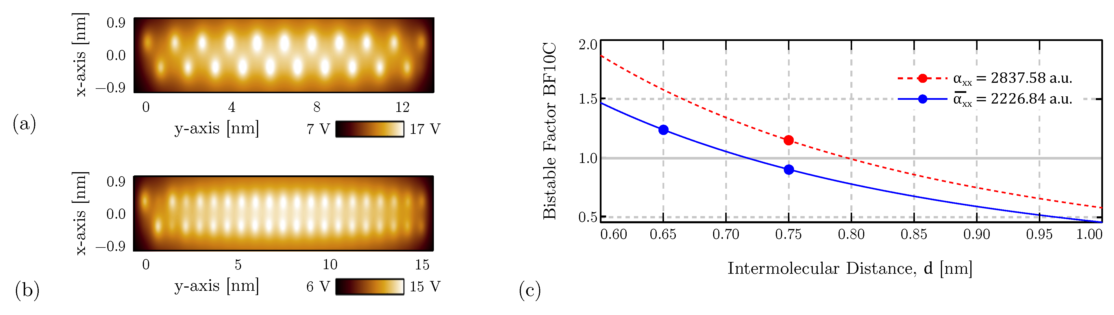
4.4. Bistability Study

So far, we considered simple systems with one or two molecules. Two molecules can be used to encode some logic information, whereas long molecular wires propagate it. Concerning the interaction among many molecules, the charge distribution of each molecule depends on the interaction among all the molecules of the wire. In particular, the propagation can be, as already explained in Section 2.2, bistable or evanescent. The propagation is named bistable when the charge distribution alternates on adjacent molecules, see Figure 11a, whereas it is evanescent when the charge separation among logical dots fades after a few molecules on the propagation direction, Figure 11b.
We defined in Section 2.2 the so-called bistable factor theory, which evaluates the information propagation in N-molecule wires using the concept of bistable factor ( B F ). In this paragraph, we analyze the bistable factor theory with the proposed energy model. In the case of the bistable propagation ( B F > 1 ), we expect to find two energy minima in the configurations of the molecular charge distribution associated with the two logical values. On the other side, if the propagation is evanescent ( B F < 1 ), we expect to find a single energy minimum in a configuration that does not propagate information.
The so-called centered bistable factor evaluated considering the interaction of 10 molecules ( B F 10 c ) can be obtained from Equation (3). Since the dipole-field relation is linear for small fields, Figure 9b, B F 0 can be derived from Equation (2) using the linear assumption described in [31].
B F 0 ( d , L , α x x ) = α x x 2 π ε 0 L 2 1 d 1 d 2 + L 2
For the diallylbutane, the width (L) equals the distance between atoms C5 and C8, see Figure 9, therefore L = 0.634 nm. The effective polarizability is considered α ¯ x x = 2226.84 a.u. to take into account the non-uniformity of the field generated by molecules. The possibility to have bistable propagation, considering a precise molecule, mainly depends on the chosen intermolecular distance. Figure 11c shows the bistable factor as a function of the intermolecular distance (d) either using the corrected polarizability ( α ¯ ) or the uniform polarizability ( α = 2837.58 a.u.). As expected, the lowest polarizability (i.e., the lower tendency of the molecule to become polar as a response to the electric field) decreases the bistable factor, eventually obstructing the information propagation.
To analyze both the bistable ( B F > 1 ) and evanescent ( B F < 1 ) propagation cases, we now focus on two precise intermolecular distances 0.65 nm and 0.75 nm, highlighted in Figure 11c with two points. We expect to find two energy minima for the 0.65 nm case, as this is supposed to favor a bistable propagation, whereas a single energy minimum for the 0.75 nm, as this is supposed to be evanescent propagation. We use the SCERPA tool to evaluate the charge distribution in a wire composed of 21 molecules. Two aggregated charges centered on atoms C5 and C8, shown in Figure 9, model the molecule electrostatic behavior. The VACT links the value of the aggregated charges to the input voltage and allows SCERPA to evaluate the intermolecular interaction. Figure 12 shows the VACT of the diallylbutane molecule, obtained from results in Section 4.3.1.
Figure 11c also reports, with a dotted line, the bistable factor evaluated with the uniform electric field polarizability ( α x x ). By using polarizability α x x with 0.75 nm distance, the bistable factor is overestimated (1.15), wrongly indicating bistable propagation. Indeed, propagation for the 0.75 nm is evanescent, as depicted by Figure 11b. This motivates the use of the effective polarizability ( α ¯ x x ) for the analysis of intermolecular interaction.
It is interesting to deepen the two cases with the proposed energy model to understand the bistable propagation under the energy standpoint and to evaluate the presence of energy minima. In this analysis, we construct a wire composed of 20 molecules. Each molecule, denoted as generic Mol-i, is modeled with two aggregated charges whose values depend on the input voltages V i n = { V 1 , , V 20 } through the VACT. The input voltages are initially set to alternate on adjacent molecules, similar to the situation of Figure 11a, following the rule:
V ¯ i n , i = 2 ( 1 ) i [ V ]
Then, the configuration is linearly changed through a parameter β to the opposite configuration V ¯ i n , that is the configuration propagating the opposite logic information, according to the equation:
V i n , i = β V ¯ i n , i
The energy of the entire wire is studied for both the intermolecular distances. For 0.65 nm, shown in Figure 13a, a 0.56 eV barrier raises between the two stable states, confirming the prediction of the bistable model. Indeed, with a short intermolecular distance, the electrostatic interaction is very high, and the exchange energy prevails on the increase of the internal energy. Concerning the 0.75 nm case, the electrostatic interaction is reduced, and the molecule polarization is not energetically favored. Indeed, no barrier appears in the energy profile. The system equilibrium and the molecule equilibrium coincide, see Figure 13b.
To conclude the analysis, we add a molecule (i.e., 21 molecules compose the wire) representing a possible driver forcing the logic information propagated through the wire. The driver input voltage (molecule i = 1 ) is constant to −2 V, whereas the other molecules (molecules i = 2 , , 21 ) input voltages follow Equation (22).
Figure 13c shows the energy trend with 0.65 nm intermolecular distance. The input voltage of the second molecule (first after the driver) can be evaluated with Equation (22) as V ¯ i n , 2 , that is, according to Equation (21), equal to −2 V. The input voltage for both the driver and the second molecule is the same: The two molecules have the same charge distribution. From a logical point of view, with β = 1 , the wire propagates the wrong information. From the energy standpoint, the barrier is reduced on the negative β -side, indicating a stable but less favorable situation than the result shown in Figure 13a. On the opposite β -side, the barrier is increased to 0.78 eV. In this condition, all the molecules create a zigzag-fashioned charge distribution, correctly propagating the driver logic information.
Finally, Figure 13d shows the same analysis performed with 0.75 nm distance. The driver introduces an asymmetry in the energy trend, increasing the barrier on the negative β -side and decreasing the energy barrier on the positive β -side. Nevertheless, the energy minimum still occurs for β 0 , indicating the logic information does not propagate in a bistable way. This result demonstrates the validity of the proposed energy model to analyze the information stability in the molecular FCN paradigm.

4.5. Memory Effect

The analysis depicted in Figure 13c reports an energy barrier between the two logical states that suggests a possible memory effect might be present in the wire. Indeed, if a wire propagates a specific logical value, some energy must be provided to the wire to propagate a different logical value. This problem is already well-known for the general QCA paradigm. Indeed, a clocking system is necessary to guide the information propagation, eventually erasing the information propagated in previous instants. We now want to deepen this memory effect from an energy perspective. We want to study how this effect can be influenced by the number of monostable molecules composing the wire.
At first, we repeat the analysis reported in Figure 13c by changing the number of molecules in the wire. Figure 14a shows the total energy of the N-molecule FCN wire as a function of the linear coordinate (i.e., the propagated logical value). For the sake of clarity, the energy value is normalized by subtracting W T O T evaluated for β = 1 . The driver is fixed to an input voltage favoring the molecular wire to assume configuration β = 1 . The plots show an energy barrier which decreases by decreasing the number of molecules in the wire. This result demonstrates that a large number of molecules enhances the memory effect. If the number of molecules is reduced to 4, the barrier is flattened, which implies the memory effect eventually be suppressed.
At this point, we analyze the molecular wire with the SCERPA tool. We insert the proposed energy model in the calculation procedure to evaluate the final total energy at the end of each timestep. For simplicity, since we are mainly interested in energy variations, the conformation energy w 0 is considered null.
We analyze the propagation of a 14-molecule and a 4-molecule wire using SCERPA in two precise timesteps. In the first timestep, we fix the driver molecule to propagate the logical information associated with β = 1 (from now on, named configuration [A]). Then, in the second time step, we change the driver to the opposite configuration to see if the propagated information changes or a memory effect appears. The latter case would be confirmed in the case the propagated information remains the same. The obtained configuration at the second timestep is referred to as configuration [B].
Figure 14b shows the charge distribution of the 14-molecule wire in the two configurations obtained with SCERPA. In configuration [A], the wire propagates the logic information denoted as β = 1 correctly. The final energy ( W T O T W 0 ) is 71.2578 eV. For the 14-molecule wire, as reported in Figure 14a, there is an energy barrier between the two logical configurations. By changing the driver configuration, we expect that the wire retains the information propagated in configuration [A]. We change the driver and let the molecular charge distribution evolving towards configuration [B]. In this last configuration, the charge distribution of the last molecule remains the same, thus the new logic does not propagate. It is possible to observe an aberration in the information propagation: After a few molecules, there are two molecules with the same charge distribution. The final energy is 71.3494 eV, thus 91.6 meV larger than configuration [A], where the information is correct. In this case, a clock field should be applied to the molecular wire in order to delete the previous information and allow the new logical information to propagate. In this work, we analyze the problem from an energy perspective, and we do not address the problem of the clocking mechanism, which is left as future work. The problem of propagating different logical values in a pipelined structure has been already analysed elsewhere [12].
Figure 14c shows the charge distribution of the 4-molecule wire in the two configurations obtained with the SCERPA tool. The wire correctly propagates the logic information denoted as β = 1 in configuration [A], and the final total energy ( W T O T W 0 ) is 12.7457 eV. For the 4-molecule wire, as reported in Figure 14a, there is no barrier between the two logical configurations. We expect that a variation of the driver voltage varies the propagated logical information. Indeed, configuration [B] shows a perfect propagation of the opposite information. The final energy is 12.1789 eV, 26.8 meV lower than configuration [A].
As the last analysis, we examine the 4-molecule wire to understand how the number of molecules in the wire influences the memory effect. Figure 15 reports the configuration of the wire, in terms of β , as a function of the driver molecule input voltage (i.e., the first molecule V i n ). With 4 and 5 molecules, the wire shows a hysteresis behavior, which means the wire maintains the propagated logic information when the driver is removed. This result confirms the presence of a memory effect.
Instead, the wire composed of 3 molecules does not show any hysteresis effect. This result demonstrates that a large number of molecules promotes the memory effect. Three molecules are not enough to create memory capabilities.
In conclusion, this analysis shows a memory effect in the propagation of molecular FCN wires and demonstrates how the energy model can be easily integrated into a simulation tool to understand better the propagation of the information in molecular FCN wires. All the calculations have been carried out by the SCERPA tool in a few seconds. The energy evaluation introduced a minimal overhead in the computation time, making the model suitable for emerging technologies CAD tools.

5. Conclusions

In this work, we propose a theoretical model to evaluate monostable molecule signal energy, when embedded in a molecular FCN circuit. In particular, we evaluate the energy into four contributions: The conformation energy, the polarization energy, the electric field energy, and the intermolecular energy. All the contributions have been defined, analyzed, calculated in several circumstances, and compared to the results of DFT calculation to validate the model.
The model relies on metrics derived from ab initio calculation, enabling the signal energy analysis by considering the effective molecule electrostatic behavior. The model allows obtaining results consistent and comparable to ab initio precision overcoming the need for computationally expensive calculation and enabling the eventual integration of the model in CAD tools.
We employ the energy model to understand the information propagation in the FCN paradigm, and, as an example, we demonstrate the so-called bistable factor validity, so far demonstrated only with electrostatic equations. We highlighted the presence of energetically stable states allowing the encoding and propagation of logic information when the molecular parameters (intermolecular distance, polarizability, and molecular width) provide a correct bistable factor. This result is essential to the characterization of information propagation in monostable molecules and demonstrates the proposed model allows linking the logical level to the molecular level, favoring the eventual design and realization of a possible molecular FCN prototype.

Author Contributions

Conceptualization, Y.A. and G.P.; methodology, Y.A. and G.P.; software, Y.A. and M.G.; validation, Y.A. and M.G.; formal analysis, Y.A. and G.P.; investigation, M.G. and G.P.; resources, M.G.; data curation, Y.A.; writing—original draft preparation, Y.A.; writing—review and editing, Y.A., M.G. and G.P.; visualization, Y.A.; supervision, M.G. and G.P.; project administration, M.G. and G.P. All authors have read and agreed to the published version of the manuscript.

Funding

This research received no external funding.

Institutional Review Board Statement

Not applicable.

Informed Consent Statement

Not applicable.

Conflicts of Interest

The authors declare no conflict of interest.

Abbreviations

The following abbreviations are used in this manuscript:
CADComputer-Aided Design
CMOSComplementary Metal-Oxide Semiconductor
DFTDensity Functiona Theory
ESPElectrostatic Potential
FCNField-Coupled Nanocomputing
MoSQuiToMolecular Simulator Quantum-dot cellular automata Torino
MUTMolecule Under Test
SCERPASelf-Consistent Electrostatic Potential Algorithm
TSATwo-State Approximation
QCAQuantum-dot Cellular Automata
VACTVin-Aggregated Charge Transcharacteristics

Appendix A

This section reports a short insight into the energy evaluation in general Quantum-dot Cellular Automata (QCA) theory. The Two-State Approximation approximates the 2-dot single molecule as a bi-stable quantum system. The two charge distributions enabling the logic encoding can be described as two quantum states a and b with associated wavefunctions ψ a and ψ b . The wavefunction of the molecular system, intended as a two-state quantum system:
Ψ | = c a ψ a | + c b ψ b |
The Hamiltonian operator H T S A :
H T S A = H a a γ γ H b b
where H a a and H b b are the energies of the two states, whereas γ is the matrix element coupling the two states. If the system is symmetrical, the two contributions are equal: H a a = H b b = H 0 . H 0 is the on-site energy. When an external stimulus is applied, one of the two states can be favored or disfavored. From the energy standpoint, we introduce the external stimulus as a perturbation of the Hamiltonian operator δ H , which favors one state and discourages the opposite one, following the approach reported in [45].
H a a = H 0 + δ H H b b = H 0 δ H
By assuming c a 2 + c b 2 = 1 , the quantum system energy W T S A can be computed as the expected value of the Hamiltonian operator.
W T S A = Ψ | H | Ψ Ψ | Ψ = 2 c a γ 1 c a 2 + ( 2 c a 2 1 ) δ H
Figure A1 shows the obtained energy by varying the coefficient c 1 for different values of δ H . If δ H = 0 , thus no perturbation, the energy profile shows the two states being equipotential. None of the two states is favored. It is important to notice that the symmetric condition ( c a = 0 ) has the maximum energy. The system has no formal neutral state with low energy. When an external stimulus is applied, the energy of the two states changes and one state becomes favored.
Figure A1. Expectation value of the Hamiltonian operator (Energy) evaluated in a Two-State Approximation.
Jlpea 12 00013 g0a1

References

  1. Lent, C.S.; Tougaw, P.D.; Porod, W.; Bernstein, G.H. Quantum cellular automata. Nanotechnology 1993, 4, 49. [Google Scholar] [CrossRef]
  2. Turvani, G.; Tohti, A.; Bollo, M.; Riente, F.; Vacca, M.; Graziano, M.; Zamboni, M. Physical design and testing of Nano Magnetic architectures. In Proceedings of the 2014 9th IEEE International Conference on Design Technology of Integrated Systems in Nanoscale Era (DTIS), Santorini, Greece, 6–8 May 2014; pp. 1–6. [Google Scholar]
  3. Breitkreutz, S.; Kiermaier, J.; Eichwald, I.; Ju, X.; Csaba, G.; Schmitt-Landsiedel, D.; Becherer, M. Majority Gate for Nanomagnetic Logic With Perpendicular Magnetic Anisotropy. IEEE Trans. Magn. 2012, 48, 4336–4339. [Google Scholar] [CrossRef]
  4. Riente, F.; Ziemys, G.; Turvani, G.; Schmitt-Landsiedel, D.; Gamm, S.B.; Graziano, M. Towards Logic-In-Memory circuits using 3D-integrated Nanomagnetic logic. In Proceedings of the 2016 IEEE International Conference on Rebooting Computing (ICRC), San Diego, CA, USA, 17–19 October 2016; pp. 1–8. [Google Scholar] [CrossRef]
  5. Csaba, G.; Imre, A.; Bernstein, G.; Porod, W.; Metlushko, V. Nanocomputing by field-coupled nanomagnets. IEEE Trans. Nanotechnol. 2002, 1, 209–213. [Google Scholar] [CrossRef] [Green Version]
  6. Turvani, G.; Riente, F.; Cairo, F.; Vacca, M.; Garlando, U.; Zamboni, M.; Graziano, M. Efficient and reliable fault analysis methodology for nanomagnetic circuits. Int. J. Circuit Theory Appl. 2017, 45, 660–680. [Google Scholar] [CrossRef] [Green Version]
  7. Cofano, M.; Santoro, G.; Vacca, M.; Pala, D.; Causapruno, G.; Cairo, F.; Riente, F.; Turvani, G.; Roch, M.R.; Graziano, M.; et al. Logic-in-Memory: A Nano Magnet Logic Implementation. In Proceedings of the 2015 IEEE Computer Society Annual Symposium on VLSI, Montpellier, France, 8–10 July 2015; pp. 286–291. [Google Scholar] [CrossRef] [Green Version]
  8. Ng, S.S.H.; Retallick, J.; Chiu, H.N.; Lupoiu, R.; Livadaru, L.; Huff, T.; Rashidi, M.; Vine, W.; Dienel, T.; Wolkow, R.A.; et al. SiQAD: A Design and Simulation Tool for Atomic Silicon Quantum Dot Circuits. IEEE Trans. Nanotechnol. 2020, 19, 137–146. [Google Scholar] [CrossRef] [Green Version]
  9. Orlov, A.O.; Amlani, I.; Bernstein, G.H.; Lent, C.S.; Snider, G.L. Realization of a Functional Cell for Quantum-Dot Cellular Automata. Science 1997, 277, 928–930. [Google Scholar] [CrossRef] [Green Version]
  10. Tóth, G.; Lent, C.S. Quasiadiabatic switching for metal-island quantum-dot cellular automata. J. Appl. Phys. 1999, 85, 2977–2984. [Google Scholar] [CrossRef] [Green Version]
  11. Wang, R.; Pulimeno, A.; Roch, M.; Turvani, G.; Piccinini, G.; Graziano, M. Effect of a Clock System on Bis-ferrocene Molecular QCA. IEEE Trans. Nanotechnol. 2016, 15, 574–582. [Google Scholar] [CrossRef]
  12. Ardesi, Y.; Turvani, G.; Graziano, M.; Piccinini, G. SCERPA Simulation of Clocked Molecular Field-Coupling Nanocomputing. IEEE Trans. Very Large Scale Integr. (VLSI) Syst. 2021, 29, 558–567. [Google Scholar] [CrossRef]
  13. Mo, F.; Spano, C.E.; Ardesi, Y.; Piccinini, G.; Graziano, M. Beyond-CMOS Artificial Neuron: A Simulation- Based Exploration of the Molecular-FET. IEEE Trans. Nanotechnol. 2021, 20, 903–911. [Google Scholar] [CrossRef]
  14. Blair, E.P.; Liu, M.; Lent, C.S. Signal Energy in Quantum-Dot Cellular Automata Bit Packets. J. Comput. Theor. Nanosci. 2011, 8, 972–982. [Google Scholar] [CrossRef]
  15. Timler, J.; Lent, C.S. Power gain and dissipation in quantum-dot cellular automata. J. Appl. Phys. 2002, 91, 823–831. [Google Scholar] [CrossRef] [Green Version]
  16. Sill Torres, F.; Wille, R.; Niemann, P.; Drechsler, R. An Energy-Aware Model for the Logic Synthesis of Quantum-Dot Cellular Automata. IEEE Trans. Comput.-Aided Des. Integr. Circuits Syst. 2018, 37, 3031–3041. [Google Scholar] [CrossRef]
  17. Blair, E.P.; Blair, E.P.; Lent, C.S. Power dissipation in clocking wires for clocked molecular quantum-dot cellular automata. J. Comput. Electron. 2010, 9, 49–55. [Google Scholar] [CrossRef]
  18. Vacca, M.; Frache, S.; Graziano, M.; Riente, F.; Turvani, G.; Roch, M.R.; Zamboni, M. ToPoliNano: NanoMagnet Logic Circuits Design and Simulation. In Field-Coupled Nanocomputing: Paradigms, Progress, and Perspectives; Springer: Berlin/Heidelberg, Germany, 2014; pp. 274–306. [Google Scholar] [CrossRef] [Green Version]
  19. Riente, F.; Garlando, U.; Turvani, G.; Vacca, M.; Ruo Roch, M.; Graziano, M. MagCAD: Tool for the Design of 3-D Magnetic Circuits. IEEE J. Explor. Solid-State Comput. Devices Circuits 2017, 3, 65–73. [Google Scholar] [CrossRef]
  20. Wille, R.; Walter, M.; Sill Torres, F.; Große, D.; Drechsler, R. Ignore Clocking Constraints: An Alternative Physical Design Methodology for Field-Coupled Nanotechnologies. In Proceedings of the 2019 IEEE Computer Society Annual Symposium on VLSI (ISVLSI), Miami, FL, USA, 15–17 July 2019; pp. 651–656. [Google Scholar] [CrossRef]
  21. Garlando, U.; Walter, M.; Wille, R.; Riente, F.; Torres, F.S.; Drechsler, R. ToPoliNano and fiction: Design Tools for Field-coupled Nanocomputing. In Proceedings of the 2020 23rd Euromicro Conference on Digital System Design (DSD), Kranj, Slovenia, 26–28 August 2020; pp. 408–415. [Google Scholar] [CrossRef]
  22. Walter, M.; Wille, R.; Torres, F.S.; Große, D.; Drechsler, R. Verification for Field-coupled Nanocomputing Circuits. In Proceedings of the 2020 57th ACM/IEEE Design Automation Conference (DAC), San Francisco, CA, USA, 20–24 July 2020; pp. 1–6. [Google Scholar] [CrossRef]
  23. Luz, L.O.; Nacif, J.A.M.; Ferreira, R.S.; Neto, O.P.V. NMLib: A Nanomagnetic Logic Standard Cell Library. In Proceedings of the 2021 IEEE International Symposium on Circuits and Systems (ISCAS), Daegu, Korea, 22–28 May 2021; pp. 1–5. [Google Scholar] [CrossRef]
  24. Frache, S.; Chiabrando, D.; Graziano, M.; Riente, F.; Turvani, G.; Zamboni, M. ToPoliNano: Nanoarchitectures design made real. In Proceedings of the 2012 IEEE/ACM International Symposium on Nanoscale Architectures (NANOARCH), Amsterdam, The Netherlands, 4–6 July 2012; pp. 160–167. [Google Scholar] [CrossRef]
  25. Lu, Y.; Lent, C.S. A metric for characterizing the bistability of molecular quantum-dot cellular automata. Nanotechnology 2008, 19, 155703. [Google Scholar] [CrossRef]
  26. Ardesi, Y.; Gaeta, A.; Beretta, G.; Piccinini, G.; Graziano, M. Ab initio Molecular Dynamics Simulations of Field-Coupled Nanocomputing Molecules. J. Integr. Circuits Syst. 2021, 16, 1–8. [Google Scholar] [CrossRef]
  27. Rahimi, E.; Reimers, J.R. Molecular quantum cellular automata cell design trade-offs: Latching vs. power dissipation. Phys. Chem. Chem. Phys. 2018, 20, 17881–17888. [Google Scholar] [CrossRef]
  28. Pulimeno, A.; Graziano, M.; Antidormi, A.; Wang, R.; Zahir, A.; Piccinini, G. Understanding a Bisferrocene Molecular QCA Wire. In Field-Coupled Nanocomputing: Paradigms, Progress, and Perspectives; Springer: Berlin/Heidelberg, Germany, 2014; pp. 307–338. [Google Scholar] [CrossRef] [Green Version]
  29. Ardesi, Y.; Pulimeno, A.; Graziano, M.; Riente, F.; Piccinini, G. Effectiveness of Molecules for Quantum Cellular Automata as Computing Devices. J. Low Power Electron. Appl. 2018, 8, 24. [Google Scholar] [CrossRef] [Green Version]
  30. Ardesi, Y.; Wang, R.; Graziano, M.; Piccinini, G. SCERPA: A Self-Consistent Algorithm for the Evaluation of the Information Propagation in Molecular Field-Coupled Nanocomputing. IEEE Trans. Comput.-Aided Des. Integr. Circuits Syst. 2019, 39, 2749–2760. [Google Scholar] [CrossRef]
  31. Ardesi, Y.; Gnoli, L.; Graziano, M.; Piccinini, G. Bistable Propagation of Monostable Molecules in Molecular Field-Coupled Nanocomputing. In Proceedings of the 15th Conference on PhD Research in Microelectronics and Electronics (PRIME), Lausanne, Switzerland, 15–18 July 2019. [Google Scholar]
  32. Neese, F. The ORCA program system. Wiley Interdiscip. Rev. Comput. Mol. Sci. 2012, 2, 73–78. [Google Scholar] [CrossRef]
  33. Neese, F. Software update: The ORCA program system, version 4.0. Wiley Interdiscip. Rev. Comput. Mol. Sci. 2018, 8, e1327. [Google Scholar] [CrossRef]
  34. Pulimeno, A.; Graziano, M.; Abrardi, C.; Demarchi, D.; Piccinini, G. Molecular QCA: A write-in system based on electric fields. In Proceedings of the 4th IEEE International NanoElectronics Conference, Tao-Yuan, Taiwan, 21–24 June 2011; pp. 1–2. [Google Scholar] [CrossRef] [Green Version]
  35. Ardesi, Y.; Beretta, G.; Vacca, M.; Piccinini, G.; Graziano, M. Impact of Molecular Electrostatics on Field-Coupled Nanocomputing and Quantum-Dot Cellular Automata Circuits. Electronics 2022, 11, 276. [Google Scholar] [CrossRef]
  36. Sutcliffe, B.T.; Woolley, R.G. On the quantum theory of molecules. J. Chem. Phys. 2012, 137, 22A544. [Google Scholar] [CrossRef] [PubMed]
  37. Graziano, M.; Wang, R.; Roch, M.R.; Ardesi, Y.; Riente, F.; Piccinini, G. Characterisation of a bis-ferrocene molecular QCA wire on a non-ideal gold surface. Micro Nano Lett. 2019, 14, 22–27. [Google Scholar] [CrossRef]
  38. Lent, C.S.; Isaksen, B. Clocked molecular quantum-dot cellular automata. IEEE Trans. Electron Devices 2003, 50, 1890–1896. [Google Scholar] [CrossRef]
  39. Atkins, P.W.; Paula, J.D. Physical Chemistry, 8th ed.; Oxford University Press: Oxford, UK, 2006. [Google Scholar]
  40. Frydel, D. Mean Field Electrostatics Beyond the Point Charge Description. In Advances in Chemical Physics; John Wiley & Sons, Ltd.: Hoboken, NJ, USA, 2016; pp. 209–260. [Google Scholar] [CrossRef] [Green Version]
  41. Singh, U.C.; Kollman, P.A. An approach to computing electrostatic charges for molecules. J. Comput. Chem. 1984, 5, 129–145. [Google Scholar] [CrossRef]
  42. Grimme, S.; Antony, J.; Ehrlich, S.; Krieg, H. A consistent and accurate ab initio parametrization of density functional dispersion correction (DFT-D) for the 94 elements H-Pu. J. Chem. Phys. 2010, 132, 154104. [Google Scholar] [CrossRef] [Green Version]
  43. Grimme, S.; Ehrlich, S.; Goerigk, L. Effect of the damping function in dispersion corrected density functional theory. J. Comput. Chem. 2011, 32, 1456–1465. [Google Scholar] [CrossRef]
  44. Weigend, F.; Ahlrichs, R. Balanced basis sets of split valence, triple zeta valence and quadruple zeta valence quality for H to Rn: Design and assessment of accuracy. Phys. Chem. Chem. Phys. 2005, 7, 3297. [Google Scholar] [CrossRef]
  45. Lu, Y.; Liu, M.; Lent, C. Molecular quantum-dot cellular automata: From molecular structure to circuit dynamics. J. Appl. Phys. 2007, 102, 034311. [Google Scholar] [CrossRef] [Green Version]
Figure 1. Basics of the molecular FCN paradigm and modelling. (a) Information encoding in Molecular FCN cells. The blue and red circles represent the location of the molecule charges; (b) propagation of the information in a molecular FCN wire composed of three cells; (c) derivation of the Aggregated charge of a 1,4-diallylbutane: DFT computed equilibrium geometry; (d) DFT computed atomic charges, colored according to the aggregation groups; (e) aggregated charges Q 1 (blue atomic charges) and Q 2 (red atomic charges).
Jlpea 12 00013 g001
Figure 2. Modelling of the molecular interaction. (a) Molecule under the effect of an electric field E i n generated by electrodes. The electric field is measured on the molecule through the so-called input voltage V i n , which is obtained by integrating E i n on a generic path connecting the two carbon atoms highlighted in blue and enlarged in the molecule; (b) molecule under test (MUT) under the effect of an electric field E i n generated by a driver molecule. The electric field is measured on the MUT through the so-called input voltage V i n . In turn, the MUT creates a second electric field E o u t which impacts other molecules. A fictitious molecule position at the same distance as the driver molecule can be exploited to evaluate the MUT capability to impact other elements by evaluating the so-called output voltage V o u t , that is, the input voltage of the fictitious molecule; (c) basic scheme for the evaluation of the centered bistable factor. The MUT is positioned between two N-molecule wires (N = 4).
Jlpea 12 00013 g002
Figure 3. Basic schematic of the energy model: Two diallylbutane molecules contribute to the total energy with their conformation energy w 0 . The intermolecular interaction and the electric field E induce a dipole μ , which increases the molecule internal energy. Each molecule is fixed in the space and interact with the other molecules and with the electric field, leading to the Interaction Energy of the system w m m ( 1 , 2 ) + w E ( 1 ) + w E ( 2 ) .
Jlpea 12 00013 g003
Figure 4. Modelling of the internal energy. (a) Diallylbutane equipotential surface (3.4 V) evaluated with the molecule at the equilibrium (configuration [A]); (b) diallylbutane equipotential surface (3.4 V) of the evaluated when an electric field induces a dipole moment in the molecule (configuration [B]); (c) internal energy W m variation of the molecule when brought from equilibrium (configuration [A]) to a polarized condition (configuration [B]) with an electric field E ; (d) equivalent mechanical model used for the modelling of the molecule polarizability at the equilibrium (configuration [A]); (e) polarization of the mechanical model under the effect of an electric field E (configuration [B]).
Jlpea 12 00013 g004
Figure 5. Equilibrium configuration of the diallylbutane cation. (a) position of atoms obtained by the geometry optimization procedure; (b) electrostatic iso-potential surface evaluated at 3.4 V.
Jlpea 12 00013 g005
Figure 6. Study of the diallylbutane cation under the effect of external electric fields. (a) Schematic of the procedure for the evaluation of the molecular polarizability; (b) dipole moment obtained with DFT computation (CAM-B3LYP/def2-TZVPP) for an oxidized diallylbutane stimulated under the effect of electric field (E). The polarization α is obtained by linearly interpolating the dipole in the central region (interpolation range).
Jlpea 12 00013 g006
Figure 7. Energy study of the diallylbutane cation under the effect of external electric fields. (a) Total energy W T O T obtained with DFT calculation (CAM-B3LYP/def2-TZVPP) and with the proposed energy model for a diallylbutane molecule embedded in an electric field; (b) electric field energy w E . (c) polarization internal energy w μ obtained with the proposed model, Equation (13), and with the ideal linear assumption, Equation (9); (d) absolute error between the DFT calculated energy and the proposed model result.
Jlpea 12 00013 g007
Figure 8. Energy study of the diallylbutane cation under the effect of surrounding molecules. (a) Interaction energy of two diallylbutane molecules positioned at different distances ‘d’ evaluated with DFT (CAM-B3LYP/def2-TZVPP) and with the proposed model; (b) relative error between the model evaluated energy and the DFT calculation; (c) interaction energy of two diallylbutane molecules evaluated with DFT and with the proposed model by using several charge approximations (ESP, Mulliken and Lowdin) for describing the molecule electrostatic behaviour with the associated relative error between the proposed model and the DFT calculation; (d) relative error between the model evaluated interaction energy obtained with different charge approximations and the DFT calculation.
Jlpea 12 00013 g008
Figure 9. Analysis of the diallylbutane cation under the effect of a driver molecule. (a) Simulation scheme of the driver-molecule system used for the evaluation of the transcharacteristics, two charges aligned with atoms C5 and C8 model the aggregated charge of a possible driver molecule; (b) diallylbutane dipole computed for different input voltages using the driver-molecule system. A linear fitting enables the evaluation of the effective polarizability α ¯ x x . The plot also reports the dipole moment obtained with a uniform electric field.
Jlpea 12 00013 g009
Figure 10. The total energy of a driver-molecule system evaluated using the proposed energy model. In this calculation, the value of molecule atomic charges { Q i } is fixed to ground state values, whereas the driver charges Q D 1 and Q D 2 are varied. Under this condition, the internal energy of the molecule is constant, and the driver-molecule interaction varies. Points highlight the energy obtained with the proposed model for the ground state configuration (i.e., the driver charges used to obtain the ground state charge distribution).
Jlpea 12 00013 g010
Figure 11. Analysis of the bistable propagation. (a) SCERPA simulation of a wire composed of 21 molecules with intermolecular distance 0.65 nm. The figure reports the voltage generated by the molecule charge distribution evaluated 0.2 nm above the molecules. The zigzag positioned white spots indicate the correctness of the information propagation; (b) SCERPA simulation of a wire composed of 21 molecules with intermolecular distance 0.75 nm. The information fades after a few molecules; (c) Centered Bistable Factor (BF10c) evaluated as a function of the intermolecular distance. The use of the effective polarizability avoid overestimating the bistable factor, correctly describing the propagation of the information in molecular wires.
Jlpea 12 00013 g011
Figure 12. Vin-Aggregated Charge Transcharacteristics (VACT) of the diallylbutane. The Aggregated Charge is calculated by summing the atomic charges calculated with DFT (CAM-B3LYP/def2-TZVPP).
Jlpea 12 00013 g012
Figure 13. Energy study of molecular wires evaluated by varying the polarization of molecules between the two propagating configurations. (a) The energy of a 20 molecule wire with the intermolecular distance 0.65 nm. A barrier between the two states ( β = ± 1 ) appears, demonstrating the bistability of the two logic states; (b) the energy of a 20 molecule wire, intermolecular distance 0.75 nm. No barrier between the two states ( β = ± 1 ) appears, demonstrating that information propagation is not possible since the logic states are not stable; (c) the energy of a 21 molecule wire, intermolecular distance 0.65 nm. The first molecule polarization is constant and emulates a possible driver. The driver introduces an asymmetry in the energy trend, favoring one of the two stable states; (d) the energy of a 21 molecule wire, intermolecular distance 0.75 nm. The first molecule polarization is constant and emulates a possible driver. The driver makes the energy trend asymmetric, yet information propagation remains not possible.
Jlpea 12 00013 g013
Figure 14. Energy analysis of the bistable propagation. (a) Total energy of a wire composed by 14, 10, and 4 molecules as a function of the β parameter, i.e., as a function of the wire molecular charge distribution. The total energy is subtracted by the total energy evaluated with β = 1 for the sake of clarity. (b) SCERPA simulations of a wire composed of 14 molecules (and a driver) with an intermolecular distance of 0.65 nm. The figure reports the voltage generated by the molecule charge distribution evaluated 0.2 nm above the molecules. In timestep [A], the zigzag positioned white spots indicate the correctness of the information propagation. In configuration [B], the driver molecule is switched to propagate the opposite logical information. The new logical information does not propagate correctly as a consequence of a memory effect. (c) SCERPA simulations of a wire composed of 4 molecules (and a driver) with an intermolecular distance of 0.65 nm. The figure reports the voltage generated by the molecule charge distribution evaluated 0.2 nm above the molecules. In timestep [A], the zigzag positioned white spots indicate the correctness of the information propagation. In configuration [B], the driver molecule is switched to propagate the opposite logical information. The molecular wire well propagates the expected logical information in both configurations, with no memory effect.
Jlpea 12 00013 g014
Figure 15. Charge configuration, described in terms of β , of a molecular wire composed of 3, 4, and 5 molecules. The β parameter is plotted as a function of the driver input voltage.
Jlpea 12 00013 g015
Publisher’s Note: MDPI stays neutral with regard to jurisdictional claims in published maps and institutional affiliations.

