
Embedded Object Detection with Custom LittleNet, FINN and Vitis AI DCNN Accelerators


Embedded Vision Systems Group, Department of Automatic Control and Robotics, Faculty of Electrical Engineering, Automatics, Computer Science and Biomedical Engineering AGH, University of Science and Technology, 30-059 Krakow, Poland
*
Author to whom correspondence should be addressed.
J. Low Power Electron. Appl. 2022, 12(2), 30; https://0-doi-org.brum.beds.ac.uk/10.3390/jlpea12020030
Submission received: 4 April 2022
/
Revised: 6 May 2022
/
Accepted: 13 May 2022
/
Published: 20 May 2022
(This article belongs to the Special Issue Hardware for Machine Learning)
Abstract
:Object detection is an essential component of many systems used, for example, in advanced driver assistance systems (ADAS) or advanced video surveillance systems (AVSS). Currently, the highest detection accuracy is achieved by solutions using deep convolutional neural networks (DCNN). Unfortunately, these come at the cost of a high computational complexity; hence, the work on the widely understood acceleration of these algorithms is very important and timely. In this work, we compare three different DCNN hardware accelerator implementation methods: coarse-grained (a custom accelerator called LittleNet), fine-grained (FINN) and sequential (Vitis AI). We evaluate the approaches in terms of object detection accuracy, throughput and energy usage on the VOT and VTB datasets. We also present the limitations of each of the methods considered. We describe the whole process of DNNs implementation, including architecture design, training, quantisation and hardware implementation. We used two custom DNN architectures to obtain a higher accuracy, higher throughput and lower energy consumption. The first was implemented in SystemVerilog and the second with the FINN tool from AMD Xilinx. Next, both approaches were compared with the Vitis AI tool from AMD Xilinx. The final implementations were tested on the Avnet Ultra96-V2 development board with the Zynq UltraScale+ MPSoC ZCU3EG device. For two different DNNs architectures, we achieved a throughput of 196 fps for our custom accelerator and 111 fps for FINN. The same networks implemented with Vitis AI achieved 123.3 fps and 53.3 fps, respectively.
1. Introduction
Deep convolutional networks (DCNNs) are characterised by high accuracy, especially for applications in the area of computer vision systems. They represent state-of-the-art solutions for tasks such as classification [1], segmentation [2], object detection [3] or tracking [4]. Regardless of the application, DCNNs are characterised by a high computational complexity, both during training and inference. Network training is usually performed using GPUs (graphics processing units) or TPUs (tensor processing units) [5]. The use of these devices for inference is also a common practise. The implementation of DCNNs on these platforms is rather simple and allows high flexibility in choosing the network architecture. Furthermore, many libraries and pre-trained models are available (so-called model zoos).
GPUs, however, are devices with a high power consumption. (It should be noted that TPUs are rather less energy-hungry than GPUs. Also, so-called embedded GPUs are designed to be power efficient). Therefore, they may not always be applicable, especially for some edge devices operating within a limited energy budget (battery-powered), such as drones or autonomous electric cars. In these cases, the lowest power consumption can be achieved by using dedicated application-specific integrated circuits (ASICs). However, this approach is less flexible, as the computing architecture cannot be changed after production. A solution with a relatively low power consumption but still high flexibility is FPGAs (field-programmable gate arrays). Their structure is based on LUTs (look-up tables), FF (flip-flop), block memories (BRAM), arithmetic-logic units (DSP) and configurable interconnection resources. This allows for dynamic changes (reconfigurations) of functionality, also in the target device, and significantly facilitates the parallelisation of calculations. The flexibility of FPGAs allows for the implementation of different approaches to data processing; in particular, DCNNs.
We can distinguish three main categories of DCNN accelerators (presented in Figure 1):
Sequential—one general purpose accelerator or several multiplexed ones dedicated to selected layer types. Only one layer (its output) is computed at the time of processing. The processing of the next layer begins when the computation for the previous layer is complete. During layer processing, the full input feature map is available. This enables access to every element of the input data. The processing time of the whole network depends on the sum of the times for all layers.
Fine-grained—all layers are organisedinto a stream executed in parallel over time. Each layer is directly connected to the previous and the next layers, which imposes dependencies. One layer cannot continue processing if the next layer is not prepared for new data or the previous one has not provided it (if needed). Large memory resources are not required here. The throughput of the entire network depends on the slowest layer.
Coarse-grained—the processing is divided into groups of layers—blocks (specifically, one layer per block) with an accelerator for each. Each block is separated from the previous and next block with memories (RAM). These store both the input and output of the block. The block has access to the full input feature map. All layers can work in parallel as there is buffering of inputs and outputs. The result of each block is obtained after determining the output of the last layer of the block. The completion of block processing is or can be synchronised. The result of the last block is the result of the whole network. The next cycle starts with new data for the first block. The processing time depends on the throughput of the slowest block. In this architecture, it is possible to implement different processing methods for each block. In particular, a part of the blocks can be fine-grained, whereas the rest is executed by sequential/general purpose accelerators.
In this paper, we present a comparison between the three mentioned approaches for implementing DCNNs in FPGAs. We designed two different convolutional network architectures (LittleNet and YoloFINN) trained for the task of classless single object detection (SOD)—only the location and dimensions of an object are detected, but not the object’s class. As training datasets, Visual Object Tracking (VOT) [6] and Visual Tracking Benchmark (VTB) [7] were chosen. We describe the network training and the quantisation process. For the detection task, we proposed to use the GCIoU loss function. Both network architectures were implemented in an FPGA. The first, LittleNet, was designed for a dedicated coarse-grained accelerator. The second, YoloFINN, was implemented as a fine-grained one using the FINN tool from AMD Xilinx [8]. We analysed the energy consumption of the processing system, depending on the frequency and the degree of computation parallelisation. Both architectures were also implemented using the sequential approach in the Vitis AI DPU from AMD Xilinx [9]. We compared the obtained implementation and optimisation results and evaluated the accelerators on the Avnet Ultra96-V2 development board with the Zynq UltraScale+ MPSoC ZCU3EG device.
The main contributions can be summarised as follows:
- A comparison between FINN and Vitis AI—we are not aware of other papers that compare these environments. There is a comparison of a number of different acceleration methods in the paper [10]—including FINN. However, the Vitis AI environment was not available at the time of writing the publication. The authors of the paper [11] compare Vitis AI with a GPU implementation. They use selected neural network architectures adapted to the detection task. Our comparison uses the same network architecture on the same device.
- The proposal of two convolutional network architectures, LittleNet and YoloFINN, for the detection task optimised for a reconfigurable embedded computing platform. For the first one, we applied multipliers of YOLO width/height channels for anchors adjustment—a solution for the problem of anchor box sizing. We are not aware of any work using similar approaches.
- A coarse-grained accelerator for the LittleNet network. We used caching of the results of successive layers, as well as multiple use of memory blocks by selected accelerators. This allows for access to the full input feature map of a given accelerator. Furthermore, this limits the transfer with external memory. Our accelerator allows for a multi-depthwise convolution operation; it is rather a unique feature, as well as operation.
- A formulation of optimisation rules to reduce the energy consumption of a system that processes a finite dataset. The method takes into account the frequency and the degree of parallelisation of the computations.
The remainder of this paper is organised as follows. In Section 2, we discuss selected research papers that address the topic of DCNNs hardware acceleration. We then present the datasets used, their partitioning and the augmentation applied in Section 3. We have devoted Section 4 to presenting the developed LittleNet architecture, its training with selected loss functions (including GCIoU) and quantisation. For the architecture mentioned above, we developed a coarse-grained accelerator, which is described in Section 5. Furthermore, we performed an energy consumption analysis of the whole processing system with the relevant experiments—Section 6. The second proposed architecture is YoloFINN, whose topology and fine-grained acceleration in FINN is presented in Section 7. In Section 8 the implementation of both architectures in the Vitis AI tool is discussed. The results obtained—speed, resource usage and energy consumption—are presented in Section 9. We compare the proposed DNNs architectures with state-of-the-art solutions in Section 10. The paper ends with a short summary with conclusions and discussion of possible future work.
2. Related Work
Due to the wide range of DNN-based applications, the issue of their hardware implementation and acceleration is often addressed in the literature. The proposed solutions are mainly targeted for FPGAs, but could also be designed as ASICs. The overview presents only selected and popular approaches to the issue. It is not possible to discuss all available solutions due to the high degree of design freedom, which makes the number of solutions almost unlimited. Frankly, each network architecture could be deployed on a custom-designed accelerator.
In the paper [12], a general purpose solution implemented as an ASIC—Eyeriss—is presented. The computations are based on an array/matrix of processing elements (PEs) connected to adjacent rows. Each PE performs a scalar product operation. To reduce energy consumption, gating is applied in the case of zero input data. Each PE is connected to a global buffer via consecutive intra-row and inter-row buses. Data transfer is carried out using the appropriate column and row tags. Additionally, compression of data exchanged with external memory was used.
The work [13] presents an improved version of the above-described solution—Eyeriss v2. The global PE array and memory have been replaced by several smaller ones. Furthermore, the configuration possibilities have been extended through configurable data and signal routing. Among other things, computational elements allowing for the calculation of so-called sparse convolutions have been used. For this purpose, data compression also occurs at the processing level. This reduces energy consumption and increases throughput.
The gating technique has also been used in the paper [14]. The authors also pointed out the problem of zero filter weights. This can be addressed already at the training stage by pruning. However, the authors also proposed the gating of zero filter weights.
The DNNBuilder framework is presented in the work [15]. The acceleration is carried out here in a fine-grained way. The network weights are read from external memory and then cached. The HybridDNN [16] environment uses a general-purpose accelerator with storing the results to external memory. In addition, the ability to perform convolutional calculations spatially and according to the Winograd algorithm was used. In the work [17], the authors proposed a coarse-grained two-stage architecture. The initial layers are realised as a fine-grained stream. In contrast, further layers are determined based on a general purpose accelerator with an on-chip buffer. The authors also presented a comparison of DNNExplorer with previous projects: DNNBuilder, HybridDNN and the commercial Xilinx Vitis AI DPU solution (architecture not stated).
The work [18] presents the DNNWaver environment. It used multiple layer accelerators with a global memory buffer. In addition, there is a local input buffer for each computational element in each block. However, the authors have not presented how the data flow between successive accelerators occurs: coarsely/sequentially using the global buffer or fine-grainedly by direct data transfer on the bus connecting the processing units (layer accelerators).
The paper [19] presents an overview of selected solutions to the DNN acceleration problem using FPGAs and ASICs, including neuromorphic platforms. The authors also address the issue of energy consumption for selected data types or memory used. An overview of the many solutions available in the literature, including FINN [8], is presented in [10]. The authors describe accelerator architectures and present a comparison, including results from source publications, for different hardware platforms, different network architectures and datasets.
In turn, the paper [11] compares implementations of selected neural networks on CPU, GPU and Xilinx DPU for the object detection task. In the case of the GPU, two number formats were used: floating-point and fixed-point. The authors describe the accelerators architectures and present a comparison, including results from source publications, for different hardware platforms, different network architectures and datasets. In the case of the GPU, two number formats were used: floating-point and fixed-point.
In the presented papers, there is no direct comparison between FINN and Vitis AI, which is one of our objectives. In addition, the comparisons that occur are mostly implemented on different platforms. In our work, we compare three types of implementations for the same task considering the limitations of the same hardware platform.
3. The Dataset Used
The training of the considered networks required a properly prepared dataset. For this purpose, we chose two sets: Visual Object Tracking (VOT2019-LT) [6] and Visual Tracking Benchmark (VTB-100) [7] and merged them. They contain tracking sequences of single objects, such as a face, a human, a car and many others. The images have different dimensions. We removed images for which no ground truth (bounding boxes) were available or the object was not visible (was outside the frame). The final size of the set was 244,795 images. We randomly divided it into three subsets in a stratified manner:
Training—117,409 images (8/15 of the whole set);
Validation—29,417 images (2/15);
Test—97,969 images (5/15).
The division used was applied to each of the subsequent training stages. For hardware evaluation, we applied only first 3000 of samples from the test set—we call it hardware test set. The reason was the reduction in evaluation time—it does not affect throughput or power. We also applied data augmentation by: vertical and horizontal reflection, rotation, additive noise in RGB, LAB and YCbCr spaces, blurring and translation. Example images are presented in Figure 2.
4. Littlenet Network
As a first step, we decided to design a network architecture with relatively low computational complexity and a low number of parameters that could be implemented relatively easily and then deployed on an embedded reconfigurable computing platform—FPGA or SoC FPGA (system on chip FPGA). We based our design on the SkyNet [20] architecture, which uses depthwise and pointwise convolutions. SkyNet was successful in the DAC SDC [21] competition (high position in the ranking). Depthwise convolution allows for the extraction of contextual features from a given pixel within a single channel. On the other hand, pointwise convolution allows one to extract features of only a given point among all of its input features. The use of the successively mentioned types of convolution is called a separable convolution. It allows us to obtain a certain approximation of the full convolution and to apply additional non-linear activation functions after each component. The result obtained is characterised by a significantly smaller number of computations and parameters.
For example, the number of parameters of the full/standard convolution with filters, context and input channels is given by Equation (1):
For a separable convolution with the same parameters, of parameters is obtained, given by Equation (2).
The value of S decreases significantly, especially for a large number of filters, and also for large kernels.
4.1. Multi-Depthwise Convolution
As mentioned above, the use of separable convolution significantly reduces the number of parameters. However, depthwise convolution allows us to perform extraction of only one context feature from the channel. For initial layers, this can be limiting or also redundantly reduce the amount of input information. To prevent this, we decided to use multi-depthwise convolution, with more filters per channel (Figure 3). This represents some compromise between separable and standard convolution. We are not aware of any other network architecture that uses this type of convolution.
4.2. Architecture
The architecture of the proposed LittleNet network is shown in Figure 4. An RGB image is given as the input to the network. The output consists of the location, size of the object and its probability of occurrence. The architecture is built of 19 blocks containing the selected convolution type (with or without bias), a normalisation layer, a possible ReLU activation function or max-pooling layer. We also used depthwise linear convolutions. This allows us to obtain features of a larger context with limiting gradient degradation. The last layer of the network is the YOLOv3-type layer [22]. The results of the next five filters form the basis for determining the validity of the pixel v—object probability, its position parameters (x, y), width w and height h. Furthermore, we applied an additional scaling of the object dimensions through trainable parameters —we called them anchor multipliers. The relationships for the parameters mentioned are described by Equations (4)–(8), where and denote, respectively, the ratio of the width and height dimensions of the input image to the dimensions of the output layer, the row and column of the output grid a-th anchor box of dimension .
In the case of multiple object detection, the value of should be thresholded to obtain a list of objects. Then, a non-maximum suppression should be applied to eliminate redundant detections. For a single-object detection task, the solution are parameters at position as an argument of the function —the highest value of the probability of object occurrence.
The numbers of filters in particular layers, parameters of multi-depthwise convolution and the number of anchor boxes were chosen experimentally. We took into account the possibility of storing all of the network weights, as well as intermediate feature maps in the internal memory of the target device (its reconfigurable part). In the same way, we selected the input dimensions of the network— (height × width). For the given input dimensions, the network output size is (height × width).
The number of parameters of the entire network equals 243,919.
4.3. Training
We trained the floating-point network by minimising the loss function given by Equation (9). Suppose that the centre of the reference object is located at point (). The loss L consists of:
- Binary cross entropy calculated for v for each anchor box. The reference mask contains the value 1 at position ().
- Mean value of bounding box regression between prediction for a-th anchor box at position (). By , we denote any loss function based on the metric.
- Regularisation as the square of the norm of all network’s parameters P.
Gciou Loss Function
Some of the loss functions more commonly used than are CIoU, DIoU [23] and GIoU [24]. During network training (for a purpose not directly related to this work), we observed that the value of , as a metric, significantly underestimates the base value of more than or . Analysing the mentioned metrics as error functions, it can be observed that has the highest value that describes the same arguments. However, as the research by the authors shows, achieves better results than . Due to the above, we decided to use a combined version of both mentioned functions. This allows us to combine the “high penalty” and expansive nature of (as well as its early extinction) with the good convergence, centrality of and the dimensions scaling of . The proposed function GCIoU (generalised complete IoU) is defined by Equation (10).
is the smallest bounding box C containing bounding boxes A and B (it does not matter which one is the reference). The indices denote, in consecutive order, the coordinates of the centre of the bounding box and its dimensions and represents the coefficient proposed by the authors of [23].
To compare the aforementioned function, we trained the LittleNet architecture using the function, as well as with the coefficient: original [23] and zeroed for values of [25]. In addition, we also used the following parameter values: , and . As a learning method, we used the stochastic gradient descent with a momentum factor of 0.9 and an initial learning rate changed at each iteration according to Equation (16). By , we mean the value of the loss function (9) of the network in iteration t. The parameters were updated every 49 batches of training data, each of size 10.
The training results are presented in Figure 5. The higher error value for is noticeable. However, this seems to be natural because of the additional sum element. Analysing the course of both the metric and the loss, we can notice a larger oscillation of in the middle part of the learning stage. This is related to the “extinction” of at the moment when one object is contained in the other, as well as to the mentioned additional sum element increasing the amplitude. The final value of , for the proposed function, is slightly lower than the others. Furthermore, in the initial learning epochs, the value of for the validation set is higher for than for . This may indicate some kind of increase in the convergence rate. However, the dataset used is also not fully reliable. This is because it contains some images with incorrect and often inaccurate labels (e.g., Figure 2b). The proposed error function should be tested on a more challenging dataset, such as MS COCO. This will allow for more reliable comparison results. As an additional result from the comparison, we can note that the application of zeroing in for small values of obtained a worse result than the original version.
4.4. Quantisation
The models obtained were implemented using floating-point numbers. However, the accelerator described in Section 5 uses fixed-point operations. In order to change the format of the computation, we performed quantisation using the brevitas library [26]. We used 8-bit fixed-point quantisation as a compromise between accuracy and memory consumption in the target hardware solution. The input data are considered to be unsigned and fully fractional—0 bits of the integer part. This notation represents the normalisation also used during floating-point training. For the convolution and normalisation weights and their results, we used quantisation with a sign. To adjust the size of the fractional part depending on the layer, we used a trainable parameter (separate for each quantised stage of the network processing). Based on it, the number of bits of the fractional part was determined according to Equation (17). The value was set to 8 (width of the selected quantisation) and s denotes the sign bit and was set to 1. The function (18) returns the nearest integer in the given range. To limit the range of values of , we used the function (19). It contains a static parameter m to control the effect of on (mainly in the initial stage of training). Experimentally, we set .
Moreover, we chose the following integer approximation methods:
- —weights;
- —input data;
- —initially for intermediate results;
- —at the end of training for intermediate (and final) results.
The flow of the quantised learning process is shown in Figure 6. We performed quantisation on the model learned with the function and continued the quantised training using the same loss function. In the first learning step, we did not quantise the normalisation layer. This was to adjust the normalisation coefficients to the new ranges of values implied by the applied quantisation. Then, in epoch 36, we replaced the normalisation layers with an affine transformation and quantised them. In epoch 46, we changed the approximation method for the layer results from to . Finally, we obtained an accuracy of for the validation set and for the test set. In comparison, the floating-point model achieved an accuracy of and , respectively. The applied quantisation resulted in a reduction in bit width from 32 to 8 bits, reducing the network accuracy by only approximately .
5. LittleNet Accelerator
To implement the above-described network in a reconfigurable system, we designed a coarse-grained accelerator. Its general schematic is shown in Figure 7. We assumed that a separate accelerator would be used for each layer. We used caching the results of the layers in RAM (implemented with BRAM available in FPGA). However, to reduce the memory consumption, we used the sharing (multiplexing) of one block of RAM by several accelerators (ACCs). Finally, we obtained a macroblock structure (Figure 8). This represents an organisational division of the accelerator’s structure. A single macroblock contains up to four accelerators along with ROMs (weights) and up to two memory blocks (feature maps). We used dual-memory sharing, but other solutions are also possible—this will increase or decrease the processing time with different RAM usage. In addition, one of the read ports is shared with another macroblock. This allows data to flow between consecutive blocks.
To avoid RAM overwriting, the processing in each block is carried out sequentially in four states. They are synchronised, i.e., each macroblock is in the same state. In each state, only one accelerator can write or read to a given memory block. This is controlled by the LittleNet control unit (LN_CU). A state changes when the currently running corresponding accelerators (same index in macroblock) of all macroblocks are completed. These blocks are then deactivated. The first step to start the next state involves waking up (changing the value of the pin from 1 to 0) the corresponding ROMs from the power saving mode. The aforementioned mode allows for a reduction in energy consumption when the ROMs are not actively used. The wake up takes a dozen clock cycles. (The documentation [27] states that two clock cycles are enough to wake up the BRAM block from sleep mode.) After this time, the ROMs are available for use. The corresponding accelerators are then turned on, and the ROMs used in the previous processing state are put to sleep. The entire process is repeated recursively as long as input data are available and output data are received.
We distinguished five types of layer accelerators:
- Input layer (IL);
- Output layer (OL);
- Depthwise convolution layer (DW);
- Pointwise convolution layer (PW);
- Max finder layer (MF).
Furthermore, we applied the grouper unit (GU) and memory writer unit (MWU) modules in each layer (Figure 9).
5.1. Grouper Unit
The schematic of the grouper unit is shown in Figure 9a. It contains a serial-parallel register (SPR) and a counter for valid input data. When the counter obtains an appropriate value, the data stored in the registers are considered valid. This allows single bytes to be grouped into double words or other multiples of input data (in the diagram, the next G bytes of data).
5.2. Memory Writer Unit
The memory writer unit allows us to write data from parallel channels. A schematic of the module is shown in Figure 9b. Each channel contains the data to be written and its validity. Data from P channels are delayed by the value of the channel index. Then, for each channel, the target memory address is incremented in case of valid data. This occurs until the maximum address from the range assigned to the channel is reached. The resulting addresses, along with the data, are multiplexed. This is followed by reading from successive channels. In addition, the multiplexer counter is reset when new valid data arrive at the input. The resulting data and addresses are the input signals of the target output RAM. When the last address is reached by the address counters of all channels, the entire module is terminated. The operation of the MWU is similar to that of a parallel-serial register. Furthermore, the frequency of valid input data cannot be greater than the number of channels.
5.3. Input Layer
The layer accelerators discussed in the following subsections have been adapted to the “channel first” data representation (CHW)—in memory, the data of a given channel appear in one continuous sequence. Images coming from a camera or read from a memory card, rather, are stored in “channel last” format—the data describing a given point (pixel) is one continuous string. It is possible to change the format in software. However, the hardware execution of this operation seems to be a better solution. Furthermore, the data sent to the accelerator are in the form of an AXI4-Stream [28]. The input data must be stored in blocks of RAM.
For this purpose, we designed a suitable accelerator for the mentioned operations—input layer (IL). The scheme is shown in Figure 10. Data coming from a four-byte wide stream are grouped into three consecutive packets. This is implemented by the GU block. The accumulated data contain 12 bytes of data—4 bytes each from the R, G and B channels. These data need to be separated due to the aforementioned input ”channel last” format (the 12 bytes represent four RGB sequences). This operation is performed by the splitter unit (SU). The sorted data create three channels that go to the MWU. The address for each packet of data from each channel is determined there. Finally, the data are written to RAM. The entire process is managed by the input layer control unit (IL_CU) block.
5.4. Depthwise Convolution Layer
We implemented the depthwise (DW) convolution based on a fine-grained pipelined processing. The scheme is shown in Figure 11. The input data are read from RAM by the sliding window unit (SWU). It uses counters for the address of the input data and its position in the feature map—row, column and channel. The data are formed into a stream. In the case of the padded version, for padding elements, the incrementation of the input data address is paused and the value of 0 is inserted into the stream. Through the appropriate delay lines, the context of a given pixel is generated. Based on the position counters mentioned above, the validity of the context is determined. For multi-depthwise convolution, the data read cycle is repeated multiple times. The weights for a given filter/channel are read from ROM and stored in registers. This is carried out by the weight loading unit (WLU). While the weights are read, the rest of the accelerator components are paused.
For the stored weights and the generated context, the value of their scalar product is determined. This is carried out within the depthwise processing unit (DW_PU)—Figure 12. Here, we have used the cascade connection capability of the DSPs [29]. Each subsequent DSP performs multiplication operations and sums the result with the result from the previous element of the cascade. The delayed () weight (Wx) and context (Dx) signals, respectively, are multiplied after performing the corresponding data character expansion to higher bits. For the first DSP, it is possible to use a bias element (B), which is aligned to the multiplication result, so that the fractional parts are of the same length. The result of the last element of the cascade is limited (LIMIT) to the range resulting from the bit size of the convolution result (the intermediate result quantisation used during training). The next DSP performs the affine transformation. Transformed and delayed normalisation weights (BN) are used accordingly. The last block implements the re-limitation of the result, as well as the application of the ReLU activation function.
The convolution result already obtained for each point is grouped in the GU module. Then, the grouped data go to the single-channel MWU module. The target memory address is assigned there. Reaching the last address finishes the computation of the depthwise convolution module.
The accelerator design allows for the implementation of a convolution with an arbitrary fixed-point format for input data, weights, bias, normalisation weights, intermediate results and output data. A version with and without padding is available.
5.5. Pointwise Convolution Layer
The pointwise (PW) layer diagram is shown in Figure 13. Pointwise convolution does not require context gathering as in depthwise convolution. Instead, it is necessary to iterate through all the input data channels for each point in the feature map. This is carried out by the point streamer unit (PSU), which generates the corresponding data stream. In addition, a data validity signal and a point-ending signal are also generated. Pointwise convolution is also characterised by a larger number of weights. Using an analogous mechanism as in DW would require all weights and input data to be accumulated in registers, and the same number of DSPs to calculate the scalar product. Instead, the weights are read in a cyclic manner from the ROM. This is performed through the cyclic streamer unit (CSU). The bias and normalisation weights are read first. They are accumulated in appropriate registers. Then. the weights of the subsequent channels are read. When the last channel is reached, iteration starts from the first channel of a given filter. This creates a cyclic stream of weights. Reading “non-cyclic” weights (read only once, bias and normalisation weights stored in registers) causes some latency to the data stream. This requires the synchronisation of the streams. The pointwise control unit (PW_CU) performs this task (and general control of the acceleration operation).
The calculation of the scalar product of the two streams is performed by the pointwise processing unit (PW_PU) modules (Figure 14). Valid input data and weights are multiplied and then accumulated in the internal register of the DSP module [30]. If the incoming data are the last element of the scalar product (LAST), then the new point (NP) flip-flop is set. This allows for the accumulator to be initialised with the bias value (B). The arrival of valid data resets the NP. Also, if the data are not valid, its product is not accumulated. The NP and VALID signals are also delayed accordingly. The data obtained from the accumulation are processed analogously to those for depthwise convolution. The value is limited, normalised and finally limited again using the function.
For the resulting data pipeline, a max pooling 2D operation with stride 2 is performed. This is implemented by the max pooling unit (MPU in Figure 13). From two consecutive values, the larger one is selected. Next, it is delayed with a delay line of a dimension of half the number of columns. The output value is then compared with the input value, and the larger one is selected. If the input of the delay line is an odd row, the result is considered as the maximum in the block. This value is considered to be valid in the output stream. The resulting data are grouped into GU modules. The MWU then determines the address of the data in the target memory.
Since the convolution result is obtained relatively sparsely, it is possible to parallelise P times the computations. This requires a wider ROM that allows P weights to be read in each clock. Furthermore, P PW_PU and GU are used. MPU and MWU are used for P channels. However, P should be limited to, at most, the number of input channels. When the max pooling operation is used and the dimensions of the input feature map are even, it is possible to limit P to two or four times the base constraint. Note that not for every value of P is a shorter processing time obtained. In addition, the parameter P also affects BRAM (ROM) usage. The DSP usage is equal to , where the first value 1 indicates the DSP used by the PSU, the second value 1 indicates the multiplication and accumulation of PW_PU and indicates normalisation usage (value 1 or 0).
Similarly to the DW accelerator, static parameters for the format of the numbers may be used. Also available are versions using bias, normalisation, ReLU and max pooling ( kernel with stride , with or without ceil mode).
5.6. Max Finder
The last convolutional layer is the YOLO layer. The task of the entire network is to find only one object. This requires the successive application of the operations: —for the validity channels ( in Equation (4)) and —for the others (– in Equations (5)–(8)). We designed a dedicated accelerator—max finder unit (Figure 15)—to perform this task. The max finder streamer unit (MFSU) generates a stream of input data. For data from the stream, the column, row and anchor to which the incoming pixel belongs are determined. This is carried out by the position counter unit (PCU). The data from the stream and its position are then processed by the max finder control unit (MF_CU). This module is based on a machine of nine states. In the first state, among the validity channels of a pixel, the one with the largest value is searched. When the pixel value is larger than the previous one, the maximum value——and its position (anchor, row, and column) are updated—.
In the second state, the object parameters from the channels at the position of are determined. When the position of a given pixel in the stream is equivalent to , its value is sent to the GU and then to the MWU. This is repeated four times (for X, Y, W and H). When the entire data have been processed, the state is transitioned to the next one. In this and the next four states, the validity value, anchor index, column and row are sent to the GU. In the seventh state, waiting to write the results to the output memory occurs. In the next state, the acceleration completion flag is set and a transition is made to the idle state. The size of the output data is only eight bytes. This allows is to limit the transfer to external memory.
5.7. Output Layer
Each accelerator stores the results in block RAM. External modules (such as a processor or other processing logic) cannot access it directly, so data transfer functionality is required. This is carried out by the output layer (OL), which performs a one-byte read from the (block) RAM. The data are grouped into double words and sent over the AXI4-Stream bus. The sending of the last packet of data marks the end of the module’s operation.
5.8. Implementation
The implementation of individual components was carried out using the SystemVerilog language. We used static parametrisation of the modules. To properly connect the layer accelerators to the memory or to the master control module—LN_CU—we used the Jinja templates [31]. This allowed us to use any order and number (limited by hardware resources) of supported layers. The multi-depthwise layer accelerator first performs filtering of all channels with one filter each. In the PyTorch environment, this is carried out by first filtering one channel with all filters, and then subsequent channels. In order to obtain the correct processing results from the accelerator, we performed a reordering of the filters. This also resulted in the reordering of the output channels. The consecutive depthwise layer required an additional change in filter order. In contrast, the pointwise layers do not require a change in filter order, but only in their weights. The order of the output channels here follows the PyTorch model. Furthermore, the YOLO layer contains odd dimensions (). This does not allow for grouping the data by four bytes. To prevent this, we supplemented the layer with a sixteenth filter.
We implemented RAM and ROM in the form of a tree. The leaves of the tree are the BRAM blocks with latency 2 and width 32 bits, for RAM. For ROM, the width was determined by the applied parallelisation (equal to 1 for DW). The total latency of the tree was adjusted to the value given by the parameter. This allowed for the same memory communication latency value to be used for all layers.
We packed the accelerator as an IP core. The resulting block was connected by the AXI4-Stream interfaces with direct memory access (DMA). This allows for data exchange between the processor system (PS) and the programmable logic (PL) accelerator of the target Zynq UltraScale + MPSoC family heterogeneous chip. This is depicted in Figure 16. For the layer parallelisation shown in Table 1, the hardware acceleration results were consistent with the quantised software model. We obtained a IoU accuracy, fps throughput and J energy consumption. We conducted these measurements at 300 MHz and for the hardware test set. Furthermore, the coarse-grained latency is six accelerator processing cycles, which is equal to the number of macroblocks.
6. Energy Usage Optimisation
The use of hardware acceleration allows for a higher processing throughput. However, the additional circuit consumes energy, so it is advisable to optimise this parameter. Reconfigurable devices allow us to make changes in the developed architecture or to adjust the appropriate operating frequency of the chip. These properties allow for the accelerator to be tuned to reduce the total energy consumption. For the accelerator described in Section 5, we determined the relationships that allowed us to reduce the energy consumption.
Assume that the system power is expressed by Equation (20). By and , we denote the power of the programmable logic and the power of the processor system, respectively. As variables, we chose the computational parallelisation p of the PW layers (for simplicity, we assume the same for all layers) and the operating frequency of the reconfigurable part f.
The energy consumption e of the system needed to perform the detection process of N images reaching a throughput of is defined by Equation (21).
In Table 2, we present the approximate processing times for each layer (normalised relative to the largest). We determined them based on the number of clock cycles needed to obtain the full result. We omitted here such elements as the times of loading weights of DW convolution, bias or PW normalisation, as well as the times of waiting for the end of writing to memory (resulting from latency). Furthermore, we assumed that communication over the AXI4-Stream bus is latency-free.
Moreover, the approximate power can be expressed by (22). We assume a linear increase in power with p for the PW layers. We take the dependence of the power on frequency to be . By and , we denote the power of the accelerators (all layers of a given type) DW and PW, respectively (for acceleration using only one PW).
Table 3 presents the maximum durations of each state for the PW and non-PW layers. The DW layers (non-PW in general) computation times are much shorter compared to the duration of the state. The aforementioned state duration (as well as the whole cycle) depends on the processing times of the PW layers. In turn, these layers depend on the parallelisation p. This allows us to formulate the assumption (23), where and are constants—the base frequency and the base fps value.
The equation of energy consumption takes the form of Equation (24).
6.1. Dependence on Parallelisation
We take f as a constant and parallelisations and such that . For , to achieve less energy consumption than for , the relation (25) is required.
This inequality is always true. We can conclude that increasing the parallelisation of the computation reduces the power consumption of the system. Increasing the parallelisation is limited by the hardware resources, as well as the number of filters in a given layer.
6.2. Dependence on Frequency
We assume p as a constant and as the dynamic power without loss of generality (the power of is unknown) for Equation (24). The dependence of power on frequency f can be expressed by Equation (31) [32] and energy consumption through Equation (32).
We assume frequencies and such that . A reduction in energy consumption is possible if and only if the relation in Equation (33) is satisfied.
The relationship in Equation (37) is also true. We can conclude that increasing the frequency of the reprogrammable part reduces the power consumption of the whole system. The limitation is the maximum frequency at which the designed accelerator works properly.
6.3. Evaluation
For the determined dependencies, we conducted experiments/tests for several values of parallelisation (value sets) and at different frequencies. We also performed tests above the maximum frequency (300 MHz), for which, the system operates deterministically. The parallelisation values are given in Table 4. We present the results of the experiments in Table 5 and Figure 17. The results allow us to conclude the validity of the determined inequalities. It should also be noted that energy consumption decreased with increasing (electrical) power.
6.4. Conclusions
For both relationships presented, a higher (electrical) power and a shorter processing time are obtained. This results in a reduced energy consumption. It can be concluded that a linear increase in power, together with the same linear increase in throughput, reduces the energy consumption of the whole system. Therefore, the proposed optimisation would involve using batch processing—turning on the accelerator for a short period of time, processing the data and then turning it off. This allows us to save energy for systems where large amounts of data are processed, but not in a time-deterministic manner. However, it should be noted that real-time systems require a fast and deterministic response time, so this approach is applicable only in specific cases (when batch processing has no negative impact).
7. Finn Accelerator
FINN [8,33] is an experimental framework for the acceleration of deep neural networks in AMD Xilinx MPSoC devices. The compiler has four main components:
- Brevitas library for training quantised models;
- Finn-hlslib [34] library written in Vivado HLS C++ environment, where the key modules are implemented;
- A compiler that transforms the model description into basic modules of the finn-hlslib library;
- A driver generator for communication between the processing system and the programmable logic on the MPSoC.
The FINN environment puts some constraints on the network architecture. First, the depthwise separable convolution mechanism, which greatly reduces computational complexity, is not directly supported. In the latest version of the compiler, an experimental build of the MobileNet-v1 DCNN, which uses separable convolutions, is available. However, only a few devices are supported, and the build requires a different, architecture-specific workflow. Taking into account the above, every triplet of the LittleNet architecture (4) was replaced with a regular convolution. The ReLU activations were also replaced with the clamp function supported in FINN:
It is a function embedded in the default Brevitas quantiser used in the FINN framework. We concluded that it introduces sufficient non-linearity to the model. The resulting architecture is similar to UltraNet [35]. Furthermore, the use of additional ReLU activations did not result in an improvement in detection quality. Finally, for hardware acceleration using FINN, the architecture shown in Figure 18a was used.
One of the limitations of the compiler is also the requirement of a square input to the model. As a result of that, the training was performed for input images and, during the inference on the device, two images were fed to the model merged into one input. This may introduce slight differences in output feature maps compared to two separate inferences in ; however, no practical differences in detection quality were observed during the evaluation. For training, the loss function from Equation (9) was used with the box regression metric.
7.1. Streaming Dataflow Architecture
In the FINN accelerator, a fine-grained streaming computing architecture is used. The basic operation used by convolutional layers is a dot product, which consists of elementwise multiplication and the accumulation of products. The diagram of the elementary processing element (PE) used for dot product computation in FINN is shown in Figure 19. The processing begins with products of A-bit inputs and W-bit weights, which are stored in on-chip memory. The products are summed in parallel in an adder tree to be sequentially accumulated towards the currently computed dot product. The final result is acquired by comparing the accumulation results with values from threshold memory, which represents the activation function used. The next degree of concurrency is obtained by using P processing elements to form the MVTU (matrix-vector-threshold unit), which computes the P output channels in parallel (Figure 20).
In order to lower the convolution operation to a matrix–matrix product, an image context of the filter size must be extracted from the layer input. This is carried out by the sliding window unit (SWU), which, for a convolution kernel of size K and stride S, writes horizontal lines of the input tensor to the on-chip memory. The data are read from the memory with interleaved channels, so all channels of a given pixel are sent together in the output data stream. The interleaving allows us to avoid unnecessary buffering of the input channels in order to gather enough information to produce a single output pixel. It does not introduce errors in convolution results because of the commutative property of addition. The order of accumulating products in an image context and the results from input channels is not important. The example of an SWU operation for , , two input channels and two output channels is shown in Figure 21. Each column of the constructed image matrix contains all channels of all pixels in a single image context. The construction of the filter matrix requires no data manipulation because it is carried out offline by the proper initialisation of the on-chip weight memory during the synthesis of the design.
7.2. Folding
The choice of and P parameters determines how the filter and image matrices are partitioned between PEs and thus allows us to balance the processing speed and resource usage. Consider a convolution with input and output channels. Between subsequent convolutional layers (each consists of a SWU followed by an MVTU), a data stream of width is being sent, where and . Every PE inside the MVTU produces a single pixel of a single output channel in cycles. In addition, P processing elements can be used inside the MVTU ( and ), resulting in the processing of P rows of the filter matrix in parallel. Ultimately, all channels of a single output pixel are computed by the layer in cycles.
Another factor that we should also pay attention to is the varying spatial dimensions of processed tensors; for example, due to maxpool operations. A tensor containing pixels is processed by an MVTU in . The product represents the total layer folding and should be constant for subsequent layers in order to avoid wasting FPGA resources for PEs that have to wait for the input data or the overflowing of FIFOs between layers. The folding parameters of each layer of the used architecture are shown in Figure 18b. The first layer of the network has the most pixels to process, so maximum parallelisation with and was applied. For the second layer, PEs and SIMD lanes were used, because there are four times fewer pixels to process due to maxpooling. The rule was propagated for every next layer to maintain constant total folding, with the last layer being an exception. Here, a slight overhead of resources was applied, because the number of output channels must be divisible by P and the number of input channels by .
7.3. Training Results
As a baseline, we trained the model using eight-bit precision. The weights from this training were also used for acceleration using Vitis AI, which we describe in Section 8. The implementation of an eight-bit model using FINN would require many more resources than those available on the Ultra96-V2 target device. Thus, the model was further trained using quantisation with fewer bits. The training process is shown in Figure 22.
Using a lower precision yielded a drastic reduction in LUT utilisation, which is the main resource for the MVTU implementation. Table 6 presents the LUT utilisation and detection IoU for different levels of quantisation. In order to meet the resource constraints of the Ultra96-V2 board, the precision of weights and activations had to be lowered to four bits.
In conclusion, the FINN framework allows for theend-to-end implementation of convolutional neural networks on FPGAs, from quantisation-aware training to deployment on the target device. However, it comes with some limitations to the model architecture and an overhead in resource utilisation compared to a custom SystemVerilog implementation due to the usage of HLS.
8. Vitis AI
For thesequential acceleration type, we chose the DPU (deep learning processor unit) of the Vitis AI environment [9]. It is a general purpose accelerator and allows for the execution of many types of layers, including standard convolutional, depthwise and transposed layers, pooling layers, concatenation, normalisation, elementwise, upsampling and activation functions such as ReLU, ReLU6, LeakyReLU or softmax [36]. Implementations of functions such as the sigmoid and hyperbolic tangent are available for selected hardware platforms. For edge devices in the target architecture, up to four DPU cores can be used (limited by the resources of the chip). Moreover, it is possible to select one of eight architecture types representing different computational powers. Additional DPU parameters allow for the configuration of memory and DSP resource consumption, as well as the types of operations performed (elementwise, depthwise), channel augmentation or power configuration. During acceleration, one DPU performs operations of only one layer (merged with other selected layers). Calculations are performed on eight-bit data in a fixed-point representation with a sign. Moreover, once generated, the DPU allows for the acceleration of arbitrary architectures (based on supported operations) without the re-generation of programmable logic configuration.
The Vitis AI environment allows us to quantise and compile the trained model in one of the popular frameworks, such as PyTorch, TensorFlow or Caffe. Depending on the framework, different steps are required. For PyTorch, the quantisation step is performed using the provided programming interface on a subset of the training data. As a result, files containing information about the quantisation used and the model architecture are generated. The next stage involves compiling the quantised model for the selected DPU version. This is performed by a dedicated compiler. Finally, a file with the model representation and information about the number of network nodes and the number of subgraphs performed on the DPU, among other things, is obtained. Network architectures that contain unsupported operations are separated into subgraphs executed on the DPU or CPU, respectively.
The evaluation of the compiled model is performed using the Vitis AI Run Time library (VART) available from Python and C++ languages. In addition, the DPU-PYNQ [37] library is also available for the PYNQ environment.
Evaluation
For comparison with other accelerators, we quantised and compiled the trained model architectures in the Vitis AI environment. We performed the quantisation process on 200 images of the validation set. For the evaluation, we used the PYNQ-DPU and DPU in the configuration:
- Architecture B1600;
- High RAM usage;
- Without distributed RAM;
- Channel augmentation;
- Depthwise convolution;
- Without average pooling;
- Without elementwise multiplication;
- Activation functions: ReLU, ReLU6 and LeakyReLU;
- High DSP48 usage;
- With energy saving mode.
The chosen configuration was intended to maximise the computational power of the DPU for the available hardware resources presented in the next section. In addition, it was required to enable the acceleration of the developed DCNN architectures. During quantisation, we found that the multi-depthwise layers were not properly transformed to the quantised model. We replaced them by separating into single depthwise convolutions and then concatenating them. This is represented by the scheme in Figure 23. However, the performed transformation required changes to the subsequent layers:
- Depthwise—filters reordering;
- Pointwise—filters’ weights reordering.
In the YoloFINN model, we used activation as a value limitation in the range of . This type of operation is not directly supported by the Vitis AI environment. We replaced this function by (39).
This representation uses three depthwise convolutions with bias, a ReLU activation function for two of them and one elementwise addition operation.
We present the results of the evaluation in Table 7. The energy consumption obtained is almost linearly related to the throughput (more precisely, to the computation time). This is obviously due to the use of the same accelerator. However, the second architecture consumes more energy. This is due to both the higher computational effort—larger feature maps and more complex operations—and the lower throughput obtained.
9. Comparison of the Used Accelerators
The proposed solutions were tested on the same computing platform—the Avnet Ultra96-V2 development board. It contains the Zynq UltraScale+ MPSoC ZCU3EG chip (SoC FPGA) composed of two ARM processors and reprogrammable logic:
- 71k CLB LUTs;
- 141k CLB flip-flops;
- 360 DSP48;
- 7.6 Mb BRAM (216 × 36b blocks);
- Up to 1.8 Mb of distributed RAM.
The resources available are relatively small. This provides an additional challenge for the compared implementation methods. In addition, the entire system works under Linux from the PYNQ distribution version 2.6 suitably customised by the PYNQ-DPU library.
Experiments were carried out on samples from the hardware test set (Section 3). We measured the energy by reading the instantaneous power values from the controllers in the hardware platform accessible through the PYNQ library. The readout of the main power regulator was not available. Therefore, we measured the sum of the power of the slave regulators (all available from the PYNQ library). We determined the power consumption as the result of the product of the computation time and the average power value recorded with a period of 0.05 s. Moreover, the evaluation of all solutions was based on multi-threaded processing. Three parallel operations were implemented: data pre-processing, hardware acceleration and post-processing.
In Table 8, we present the results obtained for both compared network architectures using different acceleration methods. The effectiveness of the floating-point model and the one running in hardware is summarised, as well as the obtained throughputs and energy consumptions. In turn, the resource consumption for the selected architectures is presented in Table 9.
As a result of quantisation, the accuracy of the LittleNet architecture decreased slightly for both methods. However, this value is higher for Vitis AI. In addition, Vitis AI quantisation took significantly less time than training with quantisation. LittleNetAcc (LittleNet accelerator) achieved a significantly higher throughput and lower power consumption. However, the coarse-grained architecture consumed more resources, especially memory resources.
In the case of the YoloFINN model, the quantisation resulted in a better accuracy than Vitis AI as well. However, it should be noted here that the initial model was trained from the beginning using eight-bit quantisation, obtaining an 0.7153 accuracy for the hardware test set. For the FINN implementation, the model was also trained using four-bit quantisation, obtaining a slightly worse accuracy value. This significantly reduced the consumption of memory and DSP resources, with only a slightly higher LUT consumption. When comparing the throughputs obtained, it can be seen that a higher value is obtained for FINN. However, the applied activation function uses an operation that is not directly supported. The use of approximation here may have significantly affected the throughput.
10. Comparison with Similar Networks Architectures
A comparison of the proposed neural network architectures with state-of-the-art solutions is not fully possible due to the not so popular task of classless single object detection (SOD). Therefore, we can only present the number of parameters of the detection architectures and their special features—Table 10. Both of our proposed architectures contain the smallest number of parameters among those listed. This is a characteristic feature of the SOD problem, which is simpler than object detection. A similar order of magnitude characterises SkyNet and UltraNet. Both were designed for the same task (SOD), but trained on a different dataset. However, our proposals still have a smaller number of parameters. The designed LittleNet architecture initially assumed a hardware implementation using a coarse-grained acceleration. We based our design on SkyNet, but the dimensions of the initial layers would prevent the full feature maps from being cached in BRAM resources. Therefore, we minimised the required amount of memory by reducing the number of pointwise convolution filters and applying multi-depthwise convolution. Moreover, we applied additional coefficients to scale the anchor box sizes. This allowed us to make the detection quality independent of anchor box sizes, which is especially important for quantised networks. YoloFINN, on the other hand, is somewhat similar to UltraNet; however, it has more than twice as few parameters and a lower activation threshold of . Additionally, we list the architectures of YOLOv3-tiny and MobileNetV2 in Table 10 as solutions to the detection task with classification for mobile devices. Both have a significantly higher number of parameters, but this is determined by a much more complex task. The comparison presented cannot be considered as a complete evaluation of the proposed neural network architectures, as this was not the main objective of our work.
11. Summary
In this paper, we have compared three approaches to DCNN hardware acceleration: sequential (Vitis AI), fine-grained (FINN) and coarse-grained (LittleNet’s own accelerator). Vitis AI offers constant resource consumption that is independent of the depth of the network. Furthermore, it is possible to reuse the bitstream obtained for another network architecture. The prerequisite here is the use of operations supported by the given configuration. Certain operations that are not directly supported can be implemented using the available operations. Implementing the solution in this environment is relatively simple. It only requires static quantisation on a subset of the training data and then the compilation of the model. However, the general purpose architecture does not allow for the complete freedom of network architecture. For unsupported operations, the processing bandwidth is limited.
For acceleration with the FINN environment, we obtained a relatively low resource consumption. However, this is due to the use of a four-bit representation. The eight-bit quantisation resulted in exceeding the available Avnet Ultra96-V2 hardware resources. The use of separable convolutions proved to be more difficult than the use of more computationally complex standard convolutions. However, a relatively high throughput can be achieved.
Coarse-grained acceleration allowed for the highest throughput. However, because the implementation was of a custom design, this was the most complex and time-consuming task. The accelerator used two types of convolution, depthwise and pointwise, as well as modules for and operations. This architecture is characterised by a relatively high resource consumption. Although logical and arithmetic resources can be adapted, memory resources are determined by the dimensions of the feature maps. This limits the applicability of the solution to relatively small networks. For larger models, it is possible to increase memory sharing within macroblocks. Moreover, it should be noted that, in the case of depthwise convolution, a relatively small number of operations are obtained per element of the resulting feature map. This results in a greater demand on memory resources, of which, there are relatively few, than on logic-arithmetic resources. Using full convolutions would increase the number of operations, thereby increasing memory efficiency—a given memory element represents a more complex feature.
In order to reduce the energy consumption of the system, we have determined the dependencies on frequency and processing parallelisation. Note that they do not reduce the electrical power of the system, but, on the contrary, the power is increased. The optimisation relies on the reduction in the runtime of constant elements (such as CPU, counters or communication). Furthermore, the parallelisation condition assumes that, as the processing power increases, the processing time decreases.
Future Work
The proposed coarse-grained accelerator allows for only a few operations. This could be extended to include standard convolution. Moreover, each macroblock uses several accelerators of the same type. It is also possible to share DSPs inside a macroblock, as proposed in [41]. In our previous implementation, we used a simple dual-port RAM. This allowed for only reading and writing to a single address in memory. Using full dual-port memory will reduce the number of reads of the pointwise and standard convolution weights.
Author Contributions
The authors made the following contributions to this work: conceptualisation, M.M., M.D. and T.K.; methodology, T.K.; software, M.M. and M.D.; validation, M.M. and M.D.; formal analysis, M.M.; investigation, M.M. and M.D.; resources, M.M.; data curation, M.M. and M.D.; writing—original draft preparation, M.M. and M.D.; writing—review and editing, T.K.; visualisation, M.M. and M.D.; supervision, T.K.; project administration, T.K.; funding acquisition, T.K. All authors have read and agreed to the published version of the manuscript.
Funding
The work presented in this paper was supported by the AGH University of Science and Technology project no. 16.16.120.773 (first and second authors) and the National Science Centre project no. 2016/23/D/ST6/01389 entitled “The development of computing resources organisation in latest generation of heterogeneous reconfigurable devices enabling real-time processing of UHD/4K video stream” (third author).
Institutional Review Board Statement
Not applicable.
Informed Consent Statement
Not applicable.
Data Availability Statement
Repository of source code of software and hardware implementations available on: https://github.com/MichalMachura/LittleNet (accessed on 1 April 2022).
Acknowledgments
The authors also thank the Academic Computer Centre CYFRONET AGH for providing access to the Prometheus computing cluster.
Conflicts of Interest
The authors declare no conflict of interest.
References
- Zhai, X.; Kolesnikov, A.; Houlsby, N.; Beyer, L. Scaling Vision Transformers. arXiv 2021, arXiv:2106.04560. [Google Scholar]
- Chen, L.; Zhu, Y.; Papandreou, G.; Schroff, F.; Adam, H. Encoder-Decoder with Atrous Separable Convolution for Semantic Image Segmentation. In Proceedings of the European Conference on Computer Vision (ECCV), Munich, Germany, 8–14 September 2018. [Google Scholar]
- Bochkovskiy, A.; Wang, C.; Liao, H. YOLOv4: Optimal Speed and Accuracy of Object Detection. arXiv 2020, arXiv:2004.10934. [Google Scholar]
- He, A.; Luo, C.; Tian, X.; Zeng, W. A Twofold Siamese Network for Real-Time Object Tracking. In Proceedings of the 2018 IEEE/CVF Conference on Computer Vision and Pattern Recognition, Salt Lake City, UT, USA, 18–22 June 2018; pp. 4834–4843. [Google Scholar] [CrossRef] [Green Version]
- Google Cloud. Available online: https://cloud.google.com/tpu/docs/tpus (accessed on 1 March 2022).
- VOT2019 Chellenge|Dataset. Available online: https://www.votchallenge.net/vot2019/dataset.html (accessed on 12 December 2021).
- Visual Tracker Benchmark. Available online: http://cvlab.hanyang.ac.kr/tracker_benchmark/datasets.html (accessed on 12 December 2021).
- Umuroglu, Y.; Fraser, N.J.; Gambardella, G.; Blott, M.; Leong, P.; Jahre, M.; Vissers, K. FINN: A Framework for Fast, Scalable Binarized Neural Network Inference. In Proceedings of the 2017 ACM/SIGDA International Symposium on Field-Programmable Gate Arrays (FPGA ’17), Monterey, CA, USA, 22–24 February 2017; pp. 65–74. [Google Scholar]
- AMD Xilinx Inc.Xilinx Vitis AI. Available online: https://github.com/Xilinx/Vitis-AI/tree/1.3.2 (accessed on 24 February 2022).
- Shawahna, A.; Sait, S.; El-Maleh, A. FPGA-Based Accelerators of Deep Learning Networks for Learning and Classification: A Review. IEEE Access 2019, 7, 7823–7859. [Google Scholar] [CrossRef]
- Verucchi, M.; Brilli, G.; Sapienza, D.; Verasani, M.; Arena, M.; Gatti, F.; Capotondi, A.; Cavicchioli, R.; Bertogna, M.; Solieri, M. A Systematic Assessment of Embedded Neural Networks for Object Detection. In Proceedings of the 2020 25th IEEE International Conference on Emerging Technologies and Factory Automation (ETFA), Vienna, Austria, 8–11 September 2020; Volume 1, pp. 937–944. [Google Scholar] [CrossRef]
- Chen, Y.; Krishna, T.; Emer, J.; Sze, V. 14.5 Eyeriss: An energy-efficient reconfigurable accelerator for deep convolutional neural networks. In Proceedings of the 2016 IEEE International Solid-State Circuits Conference (ISSCC), San Francisco, CA, USA, 31 January–4 February 2016; pp. 262–263. [Google Scholar] [CrossRef] [Green Version]
- Chen, Y.; Yang, T.; Emer, J.; Sze, V. Eyeriss v2: A Flexible Accelerator for Emerging Deep Neural Networks on Mobile Devices. IEEE J. Emerg. Sel. Top. Circuits Syst. 2019, 9, 292–308. [Google Scholar] [CrossRef] [Green Version]
- Ye, L.; Ye, J.; Yanagisawa, M.; Shi, Y. Power-Efficient Deep Convolutional Neural Network Design Through Zero-Gating PEs and Partial-Sum Reuse Centric Dataflow. IEEE Access 2021, 9, 17411–17420. [Google Scholar] [CrossRef]
- Zhang, X.; Wang, J.; Zhu, C.; Lin, Y.; Xiong, J.; Hwu, W.; Chen, D. DNNBuilder: An Automated Tool for Building High-Performance DNN Hardware Accelerators for FPGAs. In Proceedings of the 2018 IEEE/ACM International Conference on Computer-Aided Design (ICCAD), San Diego, CA, USA, 5–8 November 2018; pp. 1–8. [Google Scholar] [CrossRef]
- Ye, H.; Zhang, X.; Huang, Z.; Chen, G.; Chen, D. HybridDNN: A Framework for High-Performance Hybrid DNN Accelerator Design and Implementation. In Proceedings of the 2020 57th ACM/IEEE Design Automation Conference (DAC), San Francisco, CA, USA, 20–24 July 2020; pp. 1–6. [Google Scholar] [CrossRef]
- Zhang, X.; Ye, H.; Wang, J.; Lin, Y.; Xiong, J.; Hwu, W.; Chen, D. DNNExplorer: A Framework for Modeling and Exploring a Novel Paradigm of FPGA-based DNN Accelerator. In Proceedings of the 2020 IEEE/ACM International Conference on Computer Aided Design (ICCAD), San Francisco, CA, USA, 2–5 November 2020; pp. 1–9. [Google Scholar]
- Sharma, H.; Park, J.; Mahajan, D.; Amaro, E.; Kim, J.; Shao, C.; Mishra, A.; Esmaeilzadeh, H. From high-level deep neural models to FPGAs. In Proceedings of the 2016 49th Annual IEEE/ACM International Symposium on Microarchitecture (MICRO), Taipei, Taiwan, 15–19 October 2016; pp. 1–12. [Google Scholar] [CrossRef]
- Zaman, K.; Reaz, M.; Ali, S.; Bakar, A.; Chowdhury, M. Custom Hardware Architectures for Deep Learning on Portable Devices: A Review. IEEE Trans. Neural Netw. Learn. Syst. 2021, 1–21. [Google Scholar] [CrossRef]
- Zhang, X.; Lu, H.; Hao, C.; Li, J.; Cheng, B.; Li, Y.; Rupnow, K.; Xiong, J.; Huang, T.; Shi, H.; et al. SkyNet: A Hardware-Efficient Method for Object Detection and Tracking on Embedded Systems. Proc. Mach. Learn. Syst. 2020, 2, 216–229. [Google Scholar]
- Xu, X.; Zhang, X.; Yu, B.; Hu, X.; Rowen, C.; Hu, J.; Shi, Y. DAC-SDC Low Power Object Detection Challenge for UAV Applications. IEEE Trans. Pattern Anal. Mach. Intell. 2021, 43, 392–403. [Google Scholar] [CrossRef] [PubMed] [Green Version]
- Redmon, J.; Farhadi, A. YOLOv3: An Incremental Improvement. arXiv 2018, arXiv:1804.02767. [Google Scholar]
- Du, S.; Zhang, B.; Zhang, P.; Xiang, P. An Improved Bounding Box Regression Loss Function Based on CIOU Loss for Multi-scale Object Detection. In Proceedings of the 2021 IEEE 2nd International Conference on Pattern Recognition and Machine Learning (PRML), Chengdu, China, 16–18 July 2021; pp. 92–98. [Google Scholar] [CrossRef]
- Rezatofighi, H.; Tsoi, N.; Gwak, J.; Sadeghian, A.; Reid, I.; Savarese, S. Generalized Intersection Over Union: A Metric and a Loss for Bounding Box Regression. In Proceedings of the 2019 IEEE/CVF Conference on Computer Vision and Pattern Recognition (CVPR), Long Beach, CA, USA, 15–20 June 2019; pp. 658–666. [Google Scholar] [CrossRef] [Green Version]
- Zheng, Z.; Wang, P.; Ren, D.; Liu, W.; Ye, R.; Hu, Q.; Zuo, W. Enhancing Geometric Factors in Model Learning and Inference for Object Detection and Instance Segmentation. IEEE Trans. Cybern. 2021, 1–13. [Google Scholar] [CrossRef] [PubMed]
- Pappalardo, A. Xilinx/Brevitas. 2021. Available online: https://github.com/Xilinx/brevitas (accessed on 10 March 2022). [CrossRef]
- Xilinx Inc. UltraScale Architecture Memory Resources User Guide; Technical Report UG573 (v1.13); Xilinx Inc.: San Jose, CA, USA, 2021. [Google Scholar]
- AMBA 4 AXI4-Stream Protocol Specification. Version 1.0; Technical Report. ARM Inc., 2010. Available online: https://developer.arm.com/documentation/ihi0051/a/Introduction/About-the-AXI4-Stream-protocol (accessed on 10 March 2022).
- Fu, Y.; Wu, E.; Sirasao, A. White Paper: UltraScale and UltraScale+ FPGAs, 8-Bit Dot-Product Acceleration; Technical Report WP487 (v1.0); Xilinx Inc.: San Jose, CA, USA, 2017. [Google Scholar]
- Fu, Y.; Wu, E.; Sirasao, A.; Attia, S.; Khan, K.; Wittig, R. White Paper: UltraScale and UltraScale+ FPGAs, Deep Learning with INT8 Optimization on Xilinx Devices; Technical Report WP486 (v1.0.1); Xilinx Inc.: San Jose, CA, USA, 2017. [Google Scholar]
- Jinja. Available online: https://palletsprojects.com/p/jinja/ (accessed on 20 March 2022).
- Chéour, R.; Khriji, S.; Götz, M.; Abid, M.; Kanoun, O. Accurate Dynamic Voltage and Frequency Scaling Measurement for Low-Power Microcontrollors in Wireless Sensor Networks. Microelectron. J. 2020, 105, 104874. [Google Scholar] [CrossRef]
- Blott, M.; Preußer, T.; Fraser, N.; Gambardella, G.; O’brien, K.; Umuroglu, Y.; Leeser, M.; Vissers, K. FINN-R: An end-to-end deep-learning framework for fast exploration of quantized neural networks. ACM Trans. Reconfigurable Technol. Syst. (TRETS) 2018, 11, 1–23. [Google Scholar] [CrossRef]
- FINN-HLSLIB. Available online: https://github.com/Xilinx/finn-hlslib (accessed on 10 March 2022).
- Zhang, K.; Guo, J.; Song, B.; Zhang, W.; Bao, Z. UltraNet: A FPGA-based Object Detection for the DAC-SDC 2020. 2020. Available online: https://github.com/heheda365/ultra_net (accessed on 4 May 2022).
- Xilinx Inc. Vitis AI User Guide; Technical Report UG1414 (v1.3); Xilinx Inc.: San Jose, CA, USA, 2021. [Google Scholar]
- DPU on PYNQ. Available online: https://github.com/Xilinx/DPU-PYNQ (accessed on 10 March 2022).
- Xilinx Inc. DPUCZDX8G for Zynq UltraScale+ MPSoCs Product Guide; Technical Report PG338 (v3.4); Xilinx Inc.: San Jose, CA, USA, 2022. [Google Scholar]
- Ding, S.; Long, F.; Fan, H.; Liu, L.; Wang, Y. A Novel YOLOv3-tiny Network for Unmanned Airship Obstacle Detection. In Proceedings of the 2019 IEEE 8th Data Driven Control and Learning Systems Conference (DDCLS), Dali, China, 24–27 May 2019; pp. 277–281. [Google Scholar] [CrossRef]
- Sandler, M.; Howard, A.; Zhu, M.; Zhmoginov, A.; Chen, L. Inverted Residuals and Linear Bottlenecks. In Proceedings of the IEEE/CVF Conference on Computer Vision and Pattern Recognition, Salt Lake City, UT, USA, 18–23 June 2018; pp. 4510–4520. [Google Scholar] [CrossRef] [Green Version]
- Bao, Z.; Guo, J.; Zhang, W.; Dang, H. DSCU: Accelerating CNN Inference in FPGAs with Dual Sizes of Compute Unit. J. Low Power Electron. Appl. 2022, 12, 11. [Google Scholar] [CrossRef]
Figure 1.
Schemes of DNNs accelerators: (a) sequential, (b) fine-grained and (c) coarse-grained.

Figure 2.
Merged VOT and VTB datasets. In (a), correctly marked bounding boxes are presented. (b) shows improper annotations: a fully covered object, wrong object, wrong object part, object not fully marked or inaccurately marked. Also visible are different images’ sizes.
Figure 2.
Merged VOT and VTB datasets. In (a), correctly marked bounding boxes are presented. (b) shows improper annotations: a fully covered object, wrong object, wrong object part, object not fully marked or inaccurately marked. Also visible are different images’ sizes.

Figure 3.
Multi-depthwise convolution scheme. Two input features maps are convolved with 4 filters— 2 different filters for each map. The output map contains results of all 4 convolutions—edge colour points to the input map, colour of filling is related to filter. The output features order depends on implementation strategy.

Figure 4.
LittleNet architecture’s scheme. Denotations: M × DW —depthwise convolution with kernel of size and M sets of filters, F × PW—pointwise convolution with F filters, BIAS—using bias in convolution, BN—using batch normalisation, ReLU—applying ReLU activation function, MP—max pooling 2D layer. Blocks with the same colours have similar structure.

Figure 5.
Networks’s training results with the selected loss functions. The following graphs show: (a)—loss and (b)—IoU for training data, (c)—loss and (d)—IoU for validation data. By , we have denoted the version with zero coefficient for a small value of . The obtained waveforms achieve relatively similar values of the metric. For , there is noticeably higher loss value in comparison to .

Figure 6.
The quantisation process waveforms: (a)—loss and (b)—. The red lines indicate the epochs starting the quantisation of the normalisation layers and the change in the integer approximation method from to . The introduction of quantisation for the normalisation layers does not introduce significant changes in the error value and accuracy. Changing the approximation method causes a significant increase in the error value as well as a decrease in the accuracy.

Figure 7.
LittleNet accelerator’s scheme. Connections between macroblocks are buses for reading data from previous macroblocks.
Figure 7.
LittleNet accelerator’s scheme. Connections between macroblocks are buses for reading data from previous macroblocks.

Figure 8.
Macroblock’s scheme—two shared memories (RAM and ROM) and four layer accelerators (ACC). The last macroblock in Figure 7 is not complete—only 2 accelerators are present. In addition, the output bus is connected directly to the last accelerator—the output layer. Moreover, the presence of ROM depends on the type of the accelerator.

Figure 9.
Grouper unit is presented in (a). Input signals are stored in the serial-parallel register (SPR). Next they are concatenated (CONCAT) into a wider package. (b) presents the memory writer unit. Parallel input channels () are delayed by blocks. The blocks determine the addresses for the valid data from each channel. Next, the multiplexer (MUX) iterates over channels and selects channel’s data, address and validity as output signals. The memory writer control unit (MW_CU) controls the entire module.

Figure 10.
Schematic of the input layer (IL) accelerator—receiving data from the AXI4-Stream stream, changing the “channel last” representation to “channel first”, and writing to RAM. Denotations: GU—grouper unit, SU—splitter unit (byte reordering is represented by coloured arrows), MWU—memory writer unit, IL_CU—input layer control unit.

Figure 11.
Depthwise layer accelerator scheme. The entire block depending on configuration consumes up to 10 DSP48 modules. Denotations: SWU—sliding window unit, WLU—weights loading unit, DW_PU—depthwise processing unit, DW_CU—depthwise control unit. SWU is implemented with a basic fine-grained stream method for context generation. WLU stores weights in serial-parallel register.

Figure 12.
Depthwise processing unit—cascaded connected DSPs. The design is based on [29]. The L2 and DSP10 blocks are optional depending on the configuration. The LIMIT blocks limit the input data to a range given by the fixed-point notation parameters or the applied activation. The mentioned DSP10 block implements the normalisation operation as an affine transformation. In addition, the corresponding delays of the signals are present.

Figure 13.
Pointwise convolution layer accelerator’s scheme. The input data stream is generated by the point stream unit (PSU)—the module uses proper counters to iterate over channels and determines signal of last channel of each point. Appropriate weights are streamed by the cyclic streamer unit (CSU)—incremented ADDR_CNTR (counter) is reset to ADDR_BEGIN when WEIGHT_CNTR (counter) achieves size of filter. Based on both streams, the pointwise processing units (PW_PU_x) calculate dot products. Next, the max pool unit (MPU) performs a max pool 2D operation on each channel. For each channel, for the next two elements, max function is applied. The result is properly delayed. Next, the results of subsequent lines are compared and the higher value is selected. The validity of the results and delay lines clock are dependent on the row and column of the pixel. The results are grouped in the grouper units (GU_x). For each group, the memory writer unit (MWU) assigns the memory address. The whole process is controlled by the pointwise control unit (PW_CU).

Figure 14.
Pointwise processing unit—multiplication and accumulation (MAC). The design is based on [30]. DATA, WEIGHT and BIAS are 8-bit signals that represent input feature and filter weight and bias. BN is a pair of 8-bit signals—weights ofnormalisation. LAST is a one-bit signal that is high if DATA comes from the last channel of input data. DSP1 implements the MAC operation. The new point (NP) flip-flop allows the accumulator to be initialised with a bias value. DSP1 uses internal multiplexing based on NP state and data validation signal (VALID). The L2 and DSP2 blocks are optional depending on the configuration. The LIMIT blocks limit the input data to a range given by the fixed-point notation parameters or the applied activation. The mentioned DSP2 block implements the normalisation operation as an affine transformation with delayed BN weighs by D_BN block.

Figure 15.
Max finder unit (MFU)—finding parameters of the object for the highest validity. The max finder streamer unit (MFSU) generates a data stream. For each element of the stream, the position counter unit (PCU) assigns coordinates of map and anchor positions. The max finder control unit (MF_CU) implements the main functionality—it finds coordinates of the most probable object and its parameters. The resulting single bytes of object description are grouped in the grouper unit (GU). The aforementioned description are values of the anchor channels ( and in Equations (4)–(8)), location of the object on the grid and anchor index. Next, the memory writer unit assigns the address for each group.

Figure 16.
Block design with our accelerator and inverter of reset signal highlighted—our accelerator is reset with logical 1.
Figure 16.
Block design with our accelerator and inverter of reset signal highlighted—our accelerator is reset with logical 1.

Figure 17.
Result of the experiments. Energy dependency on frequency and parallelisation. Applying higher frequencies and higher parallelism allows us to decrease total energy consumption (CPU + FPGA) for the processing of a fixed size dataset. The parallelism is limited by the available resources. The frequency is limited by the value that allows for correct results. The energy consumption saturates slightly with the increase in the frequency.

Figure 18.
(a) Convolutional architecture used in the FINN accelerator and (b) folding parameters for each layer. The number of processing elements (PE) and SIMD lanes used for each layer determines the level of parallelism. Note that the use of maxpool layers results in the reduction in spatial dimensions of the processed tensor. Therefore, fewer FPGA resources are needed for later layers of the network. For details, refer to Section 7.2.

Figure 19.
Single processing element (PE) used for dot product computation in FINN framework. Q input channels with A-bit precision are processed in parallel. The W-bit weights are stored in on-chip memory to avoid memory bandwidth bottlenecks. As a result of the fine-grained architecture of the system, the processed input pixels are accumulated sequentially before an output channel is computed. The values from the threshold memory are used for comparisons with the accumulated result to implement the required activation function.

Figure 20.
Matrix-vector-threshold unit used for fully connected and convolutional layers in FINN. The module processes the data stream generated by the sliding window unit (SWU), which reduces convolution operation to a multiplication between filter and image matrices. The columns of the filter matrix are split between SIMD lanes and each row is mapped to a different PE.

Figure 21.
The figure shows the process of reducing the convolution operation to a matrix–matrix multiplication. In this example, two-channel input is processed by four convolutional filters to produce two-channel output. The proper filter matrix is kept inside weight memory of every PE and the image matrix is constructed by the SWU during inference. The result of the convolution is a product of the filter matrix and the image matrix. Every column of the image matrix contains image context for a single filter location and each row of the filter matrix contains weights corresponding to a single output channel.

Figure 22.
The training procedure of the YoloFINN architecture. The dashed red line denotes the moment of changing the precision from 8 to 4 bits. Such level of quantisation was necessary to meet the constraints of the embedded platform.
Figure 22.
The training procedure of the YoloFINN architecture. The dashed red line denotes the moment of changing the precision from 8 to 4 bits. Such level of quantisation was necessary to meet the constraints of the embedded platform.

Figure 23.
Multi-depthwise convolution replaced by concatenated 3 single depthwise convolutions. The presented transformation allows for multi-depthwise convolution acceleration with Vitis AI DPU.
Figure 23.
Multi-depthwise convolution replaced by concatenated 3 single depthwise convolutions. The presented transformation allows for multi-depthwise convolution acceleration with Vitis AI DPU.


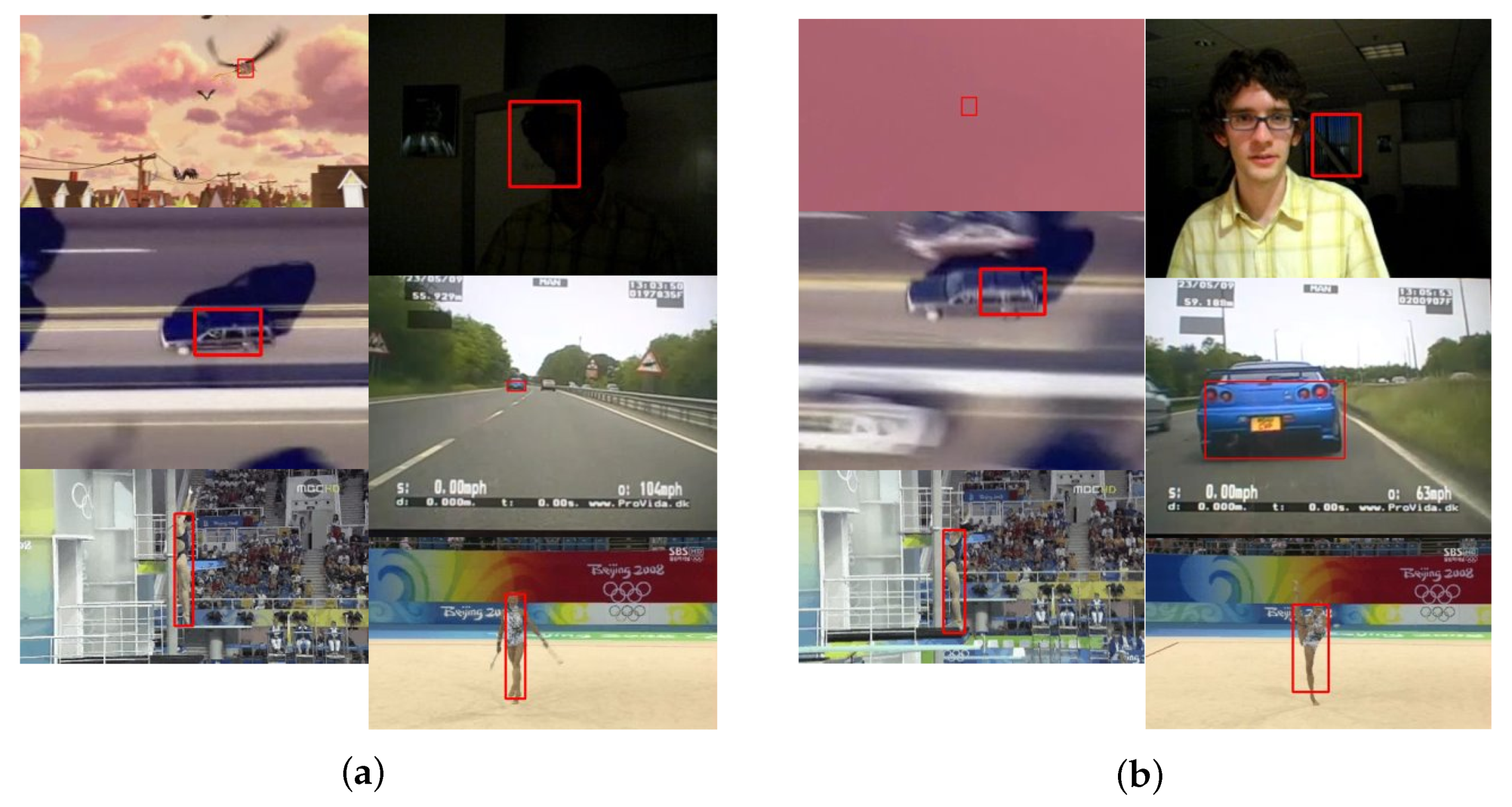
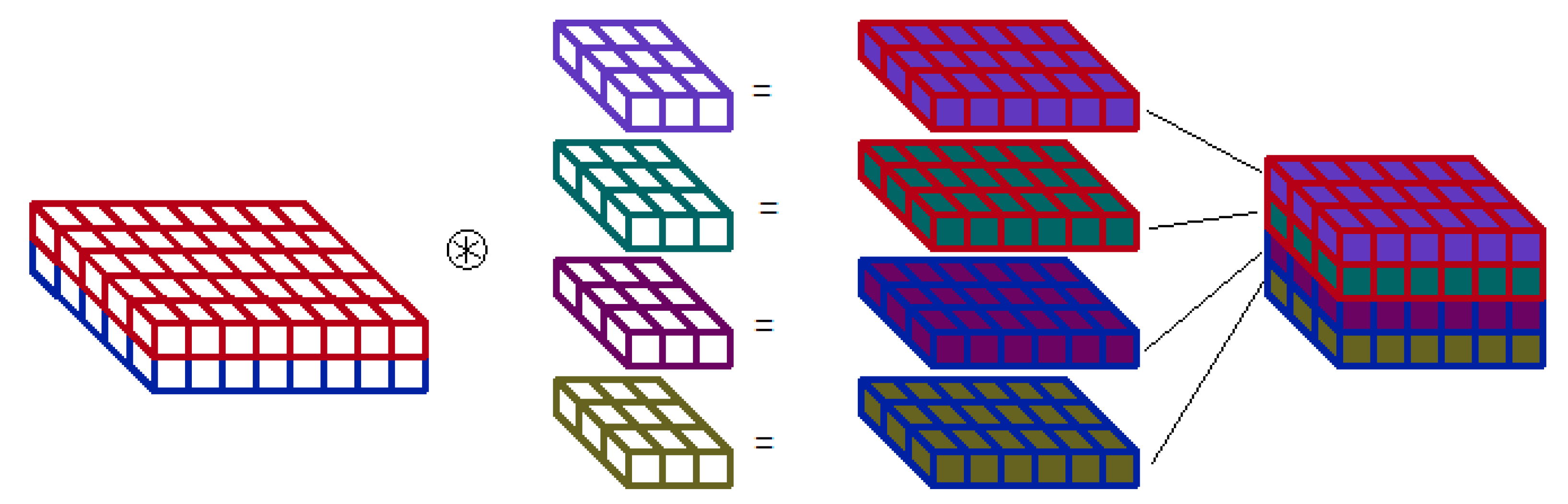
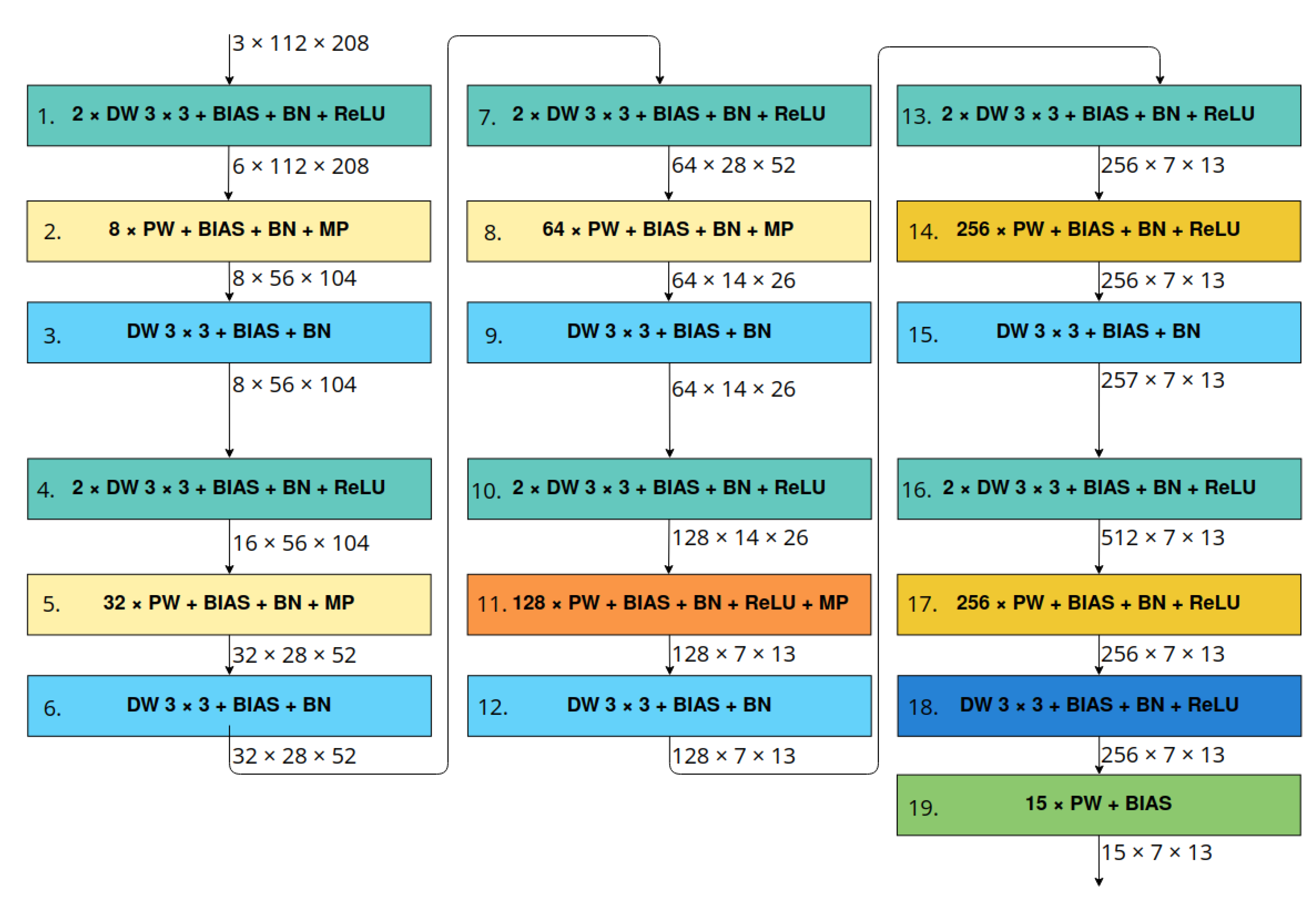
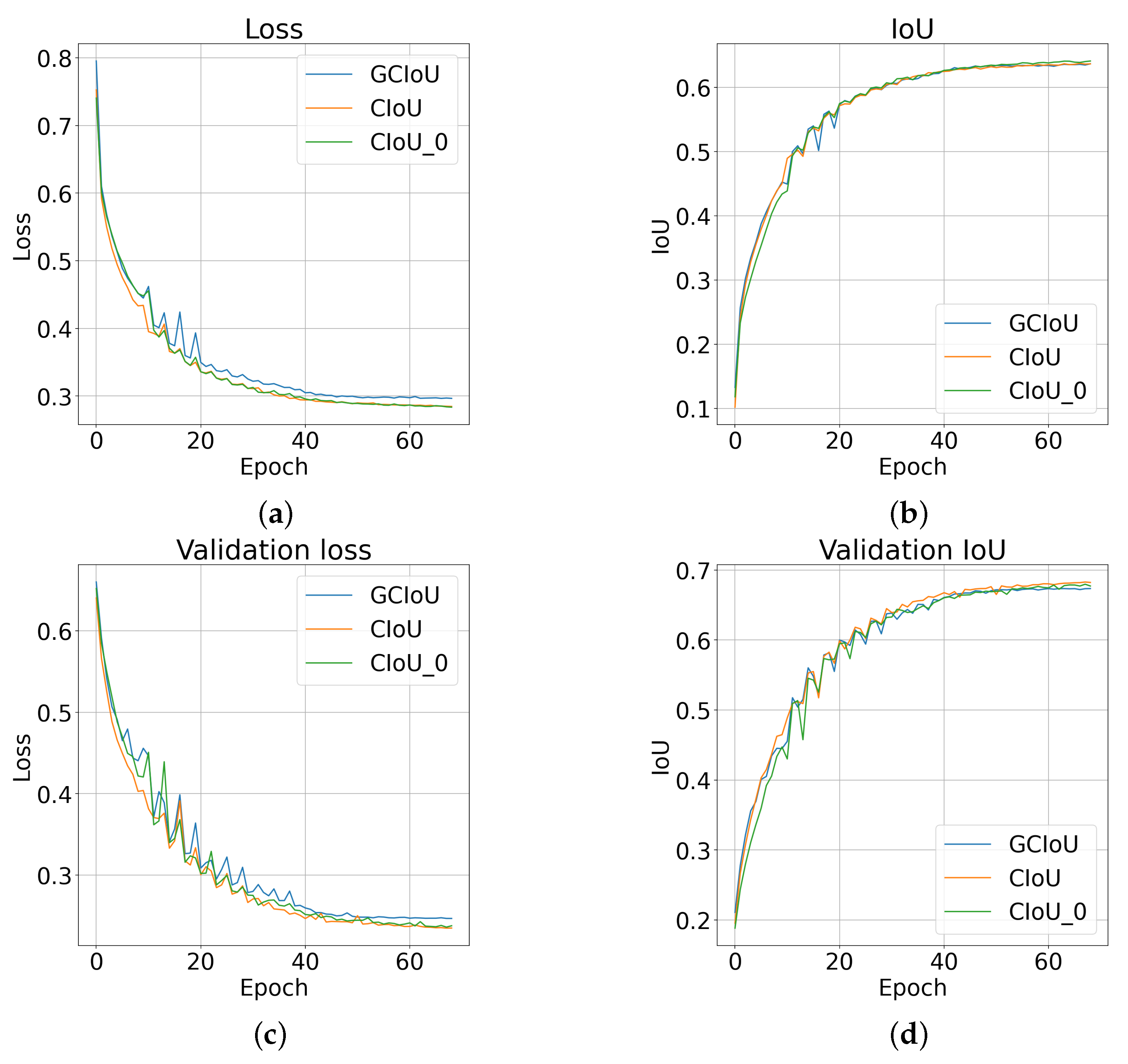
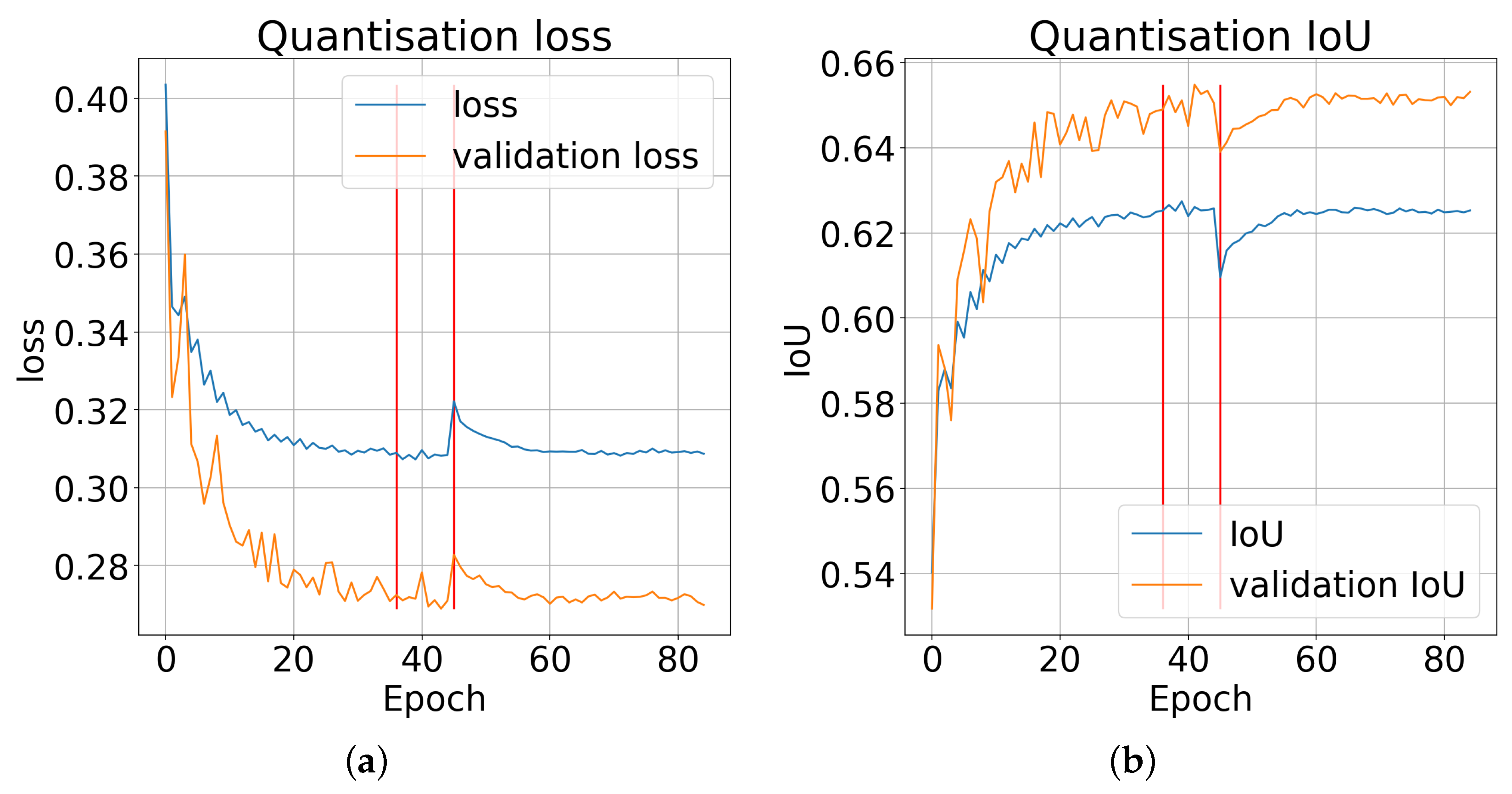
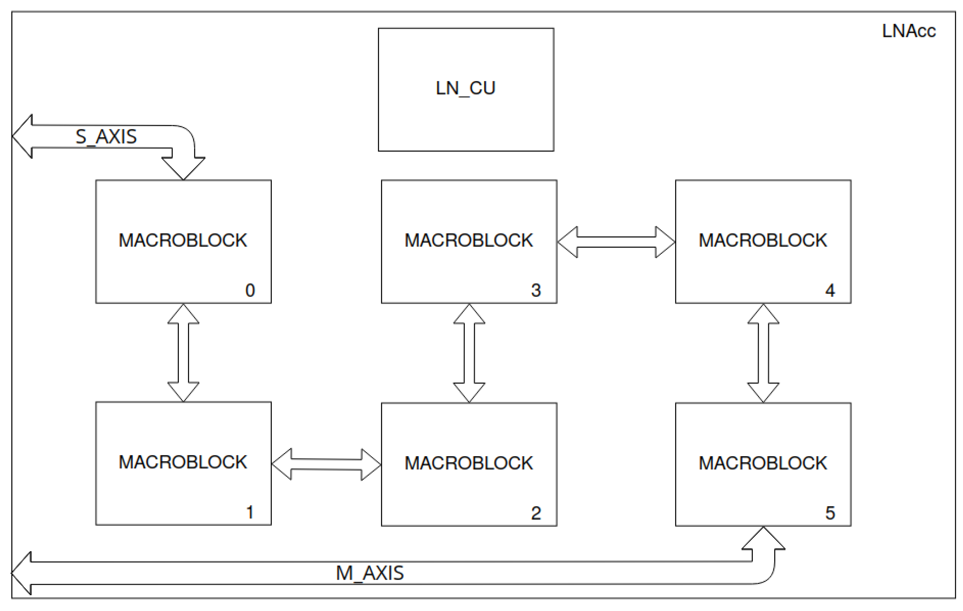
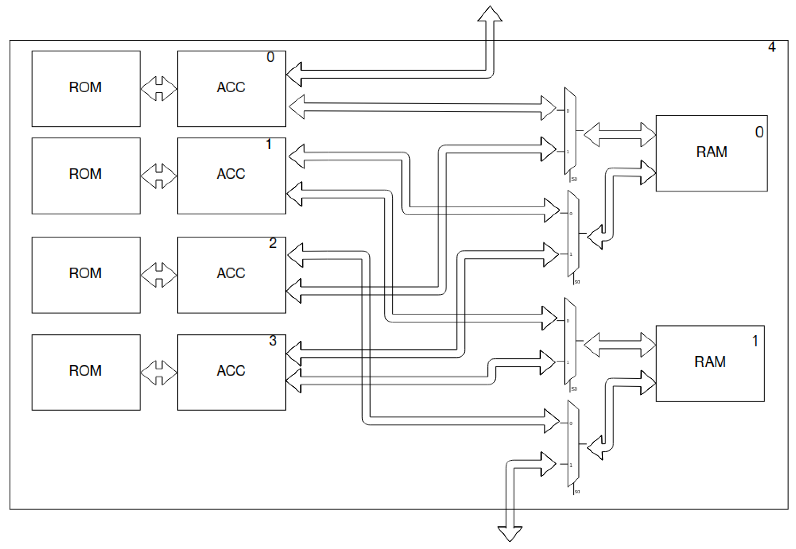
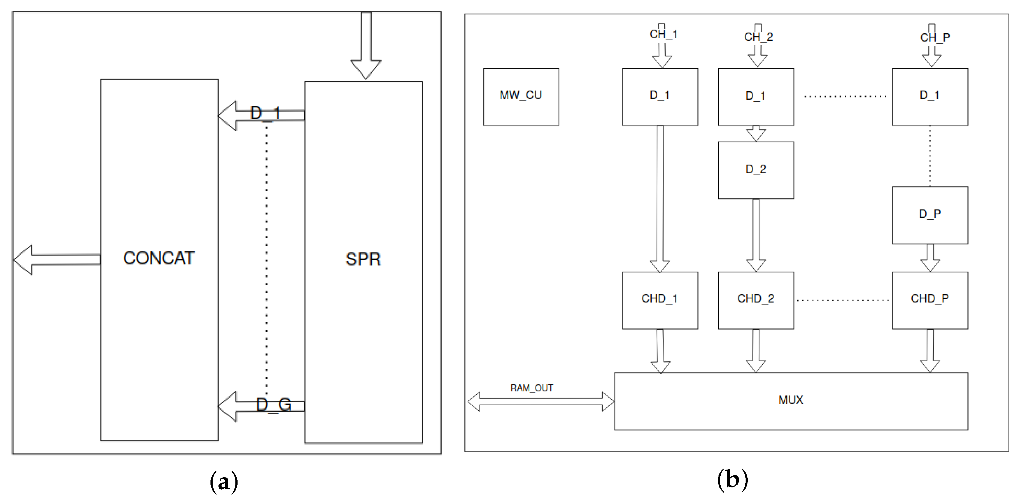
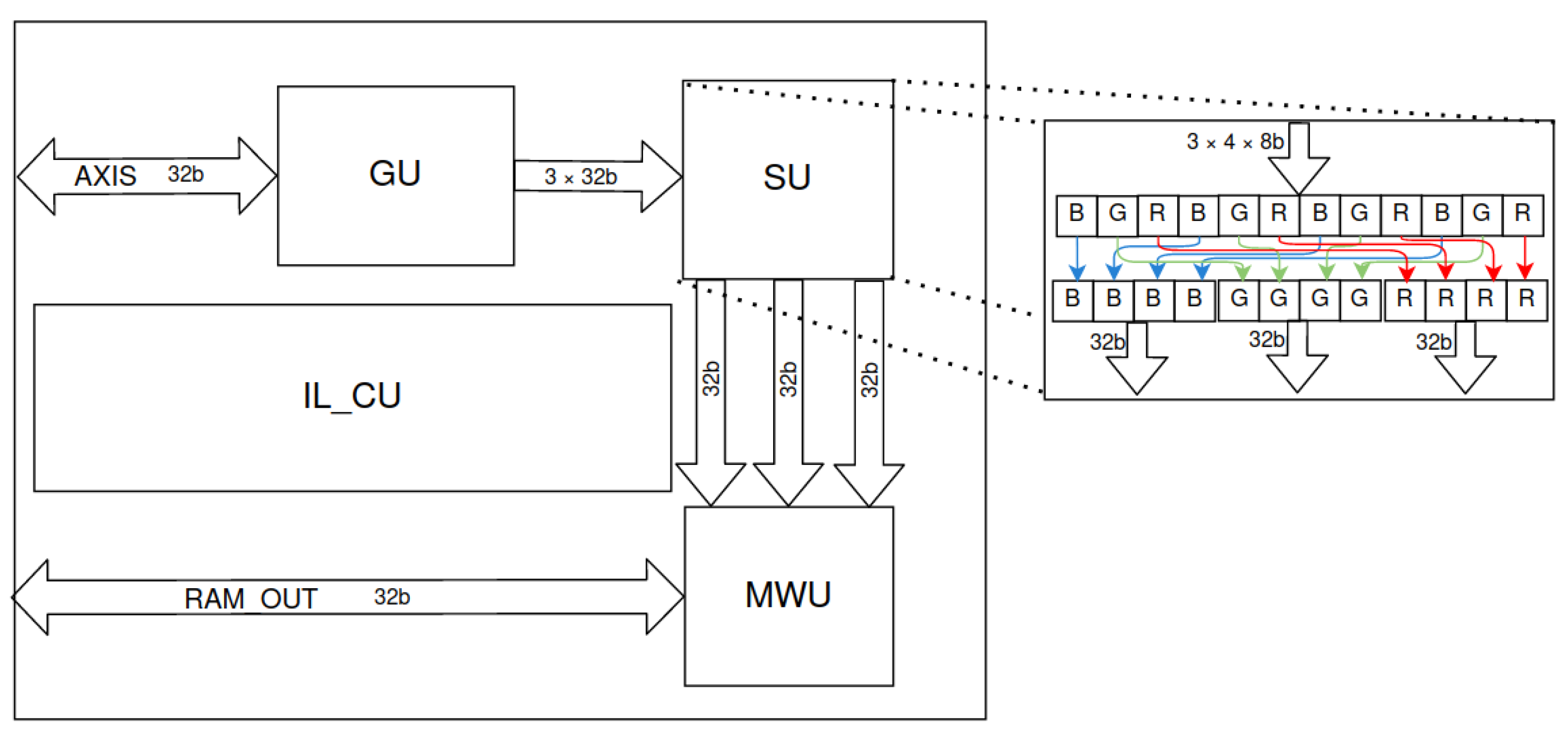
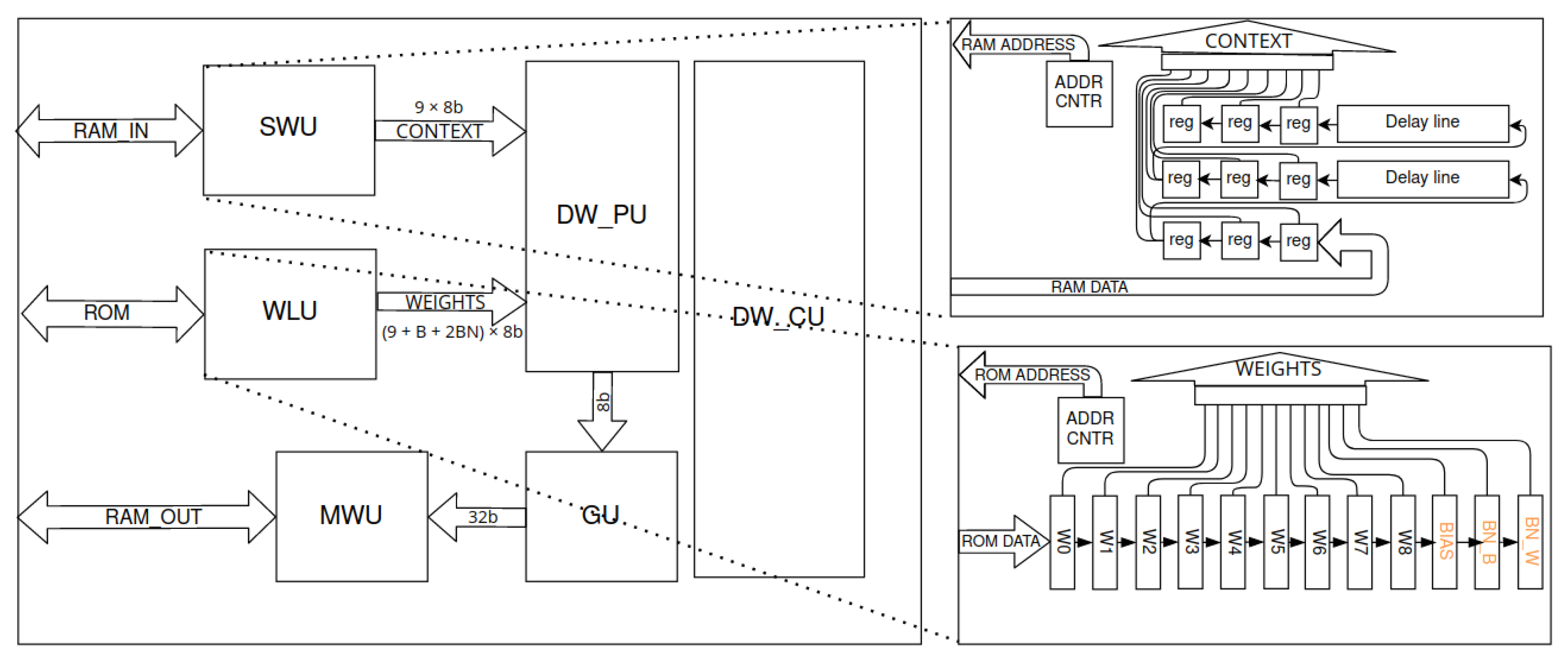
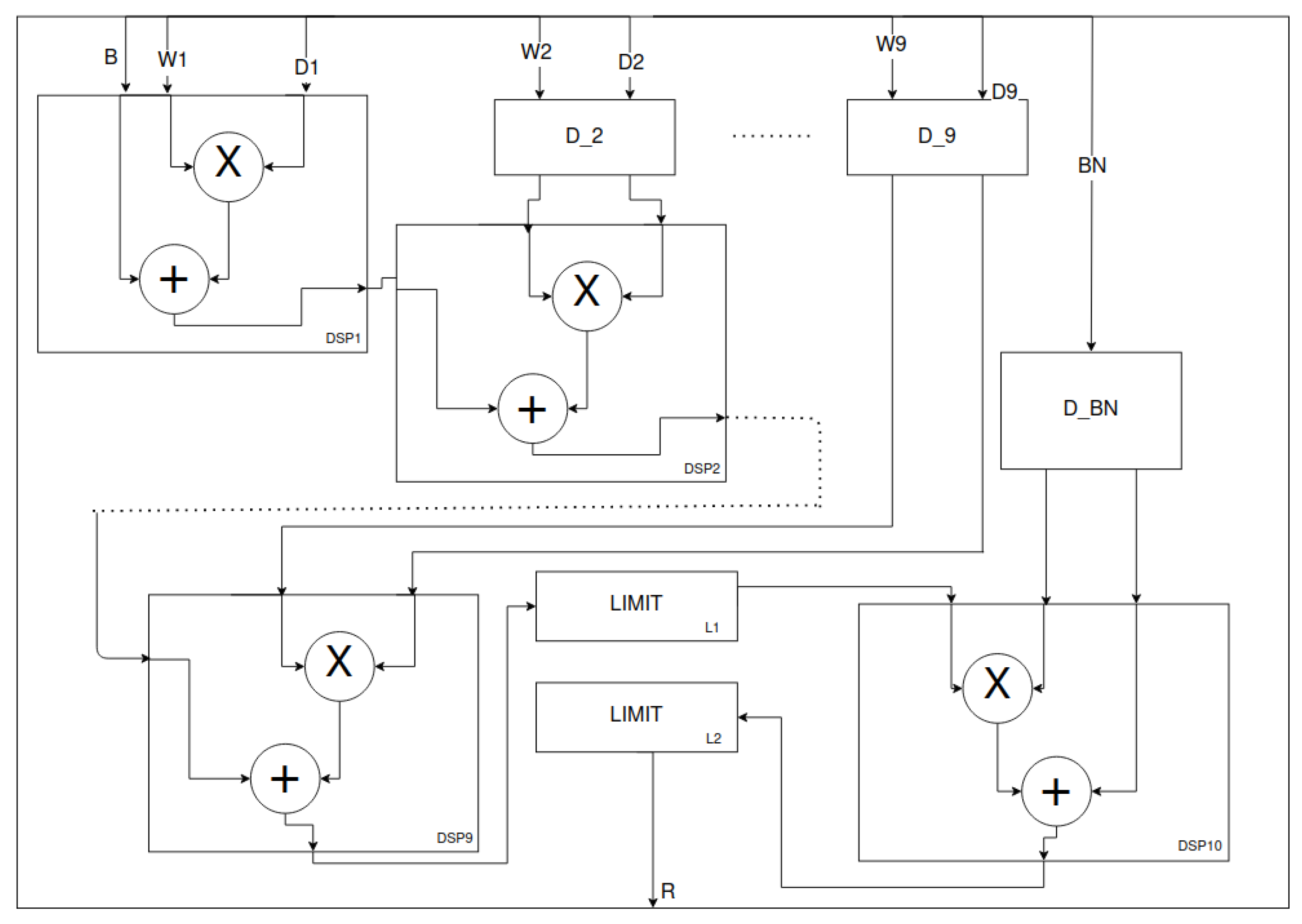
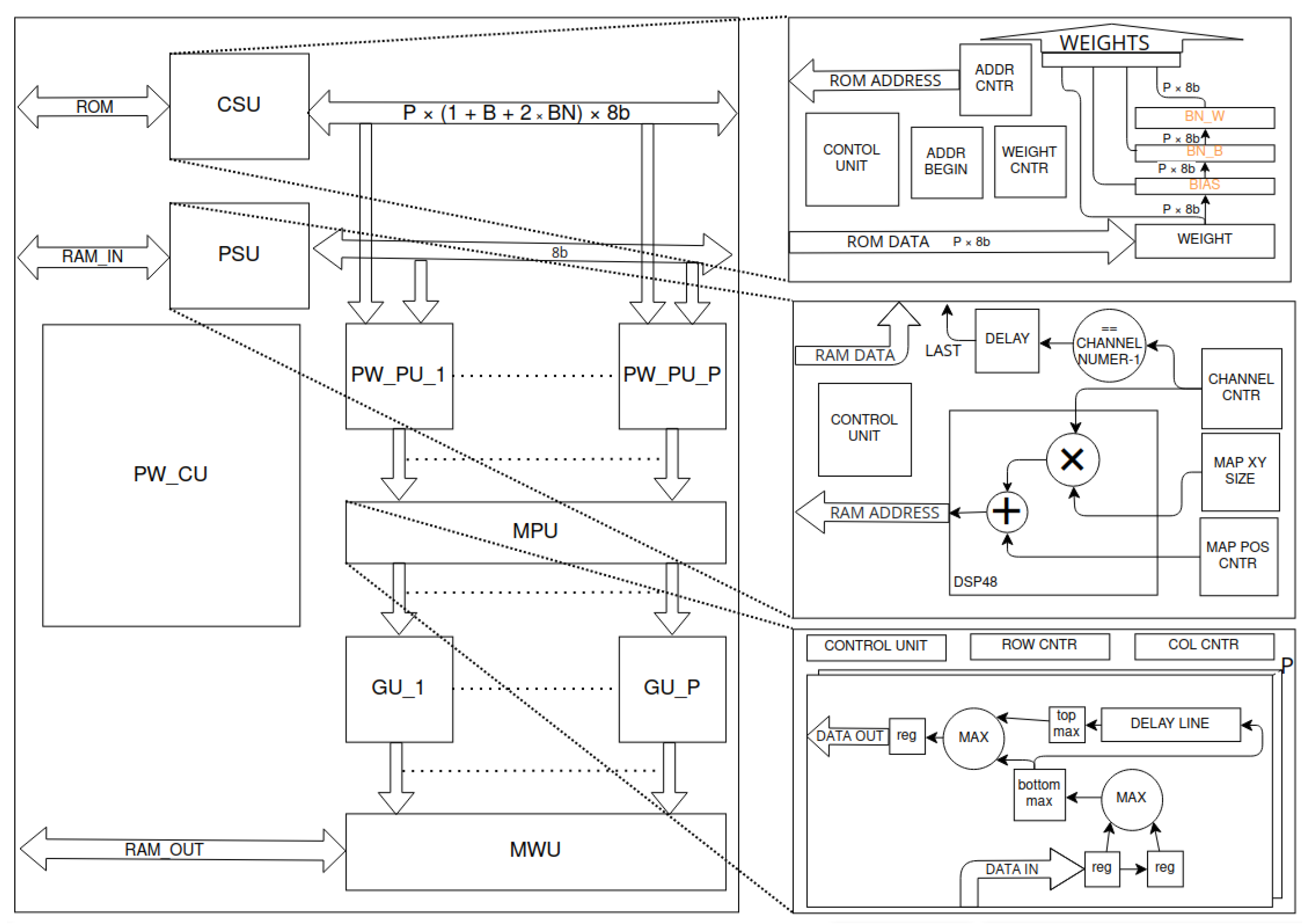
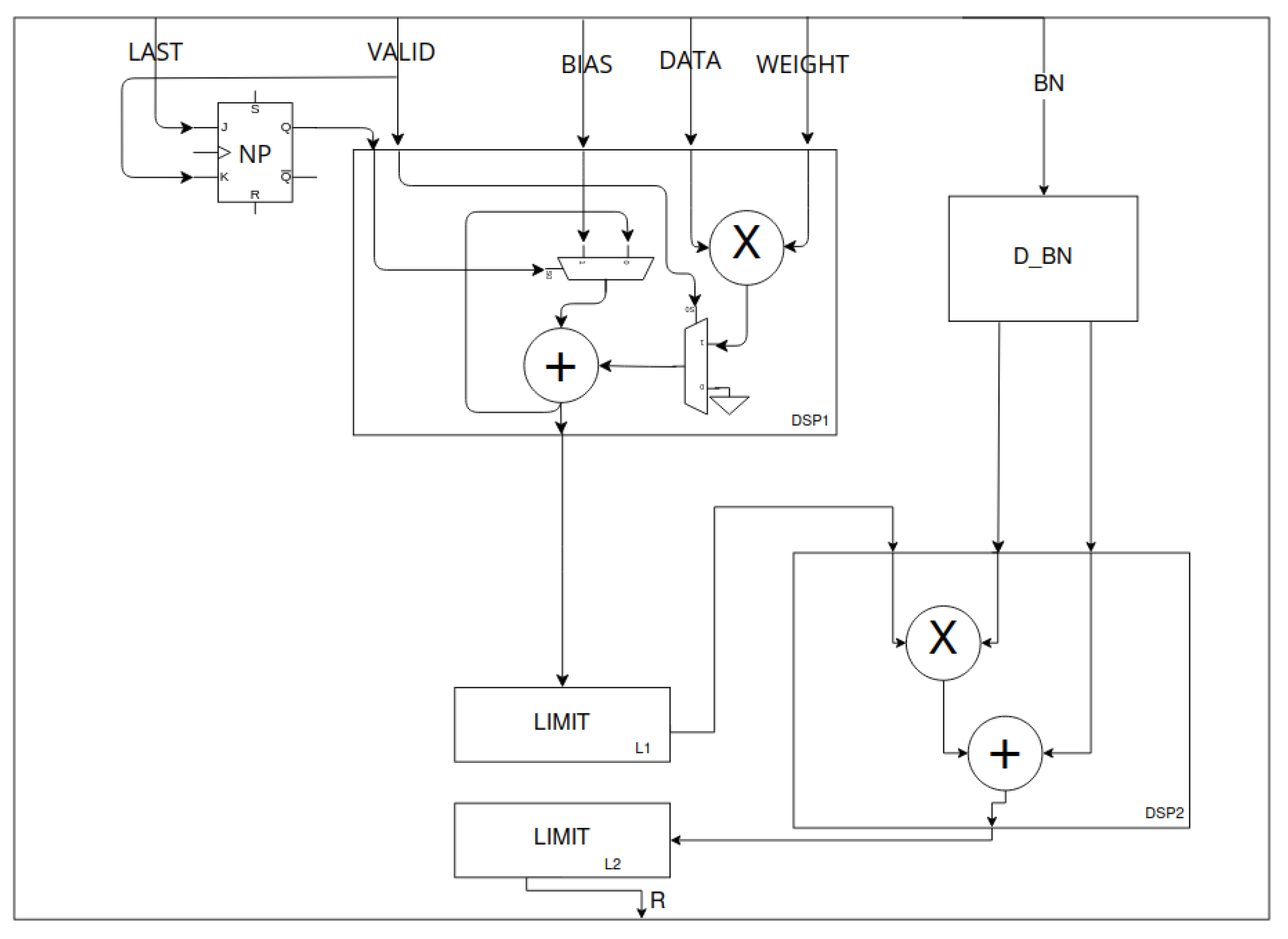
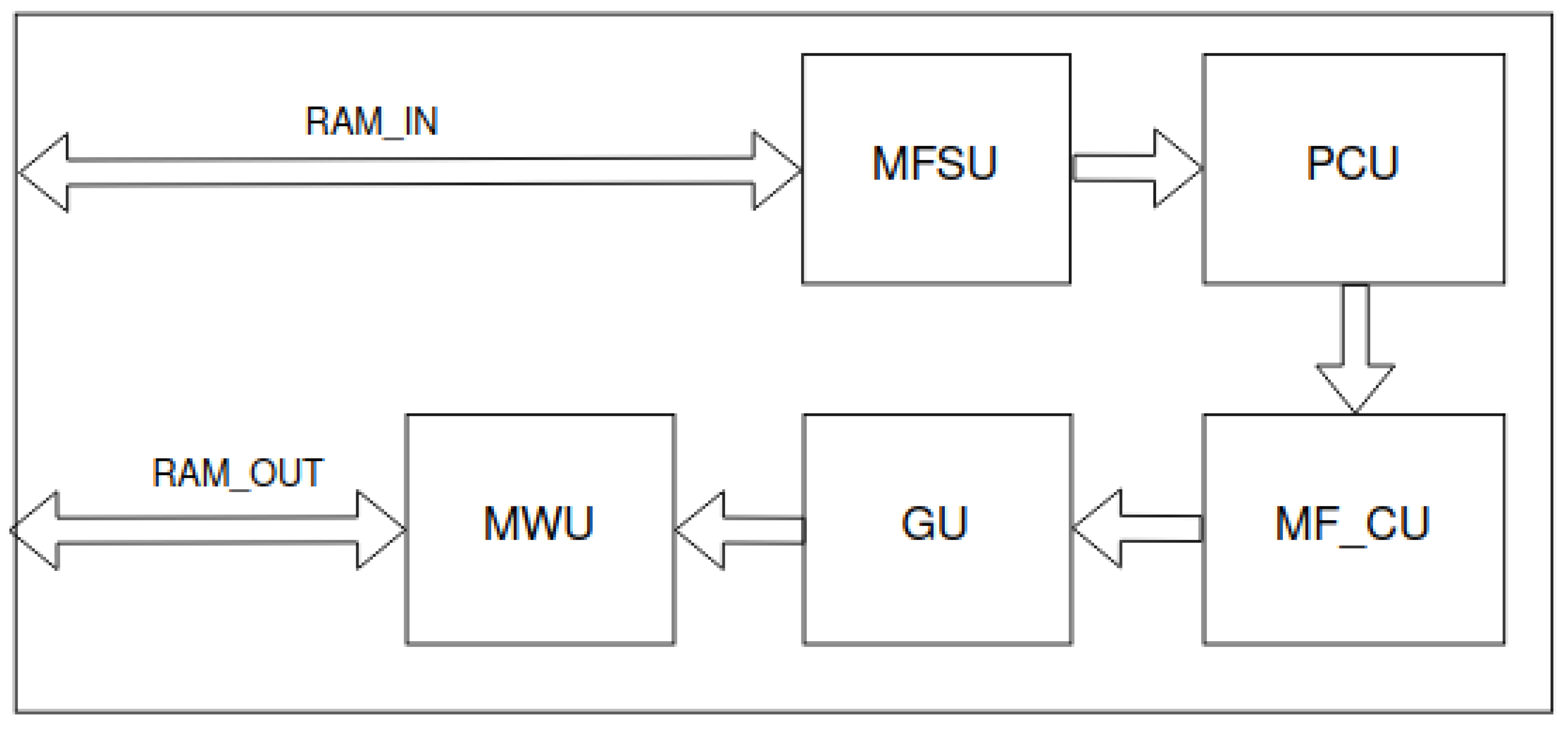
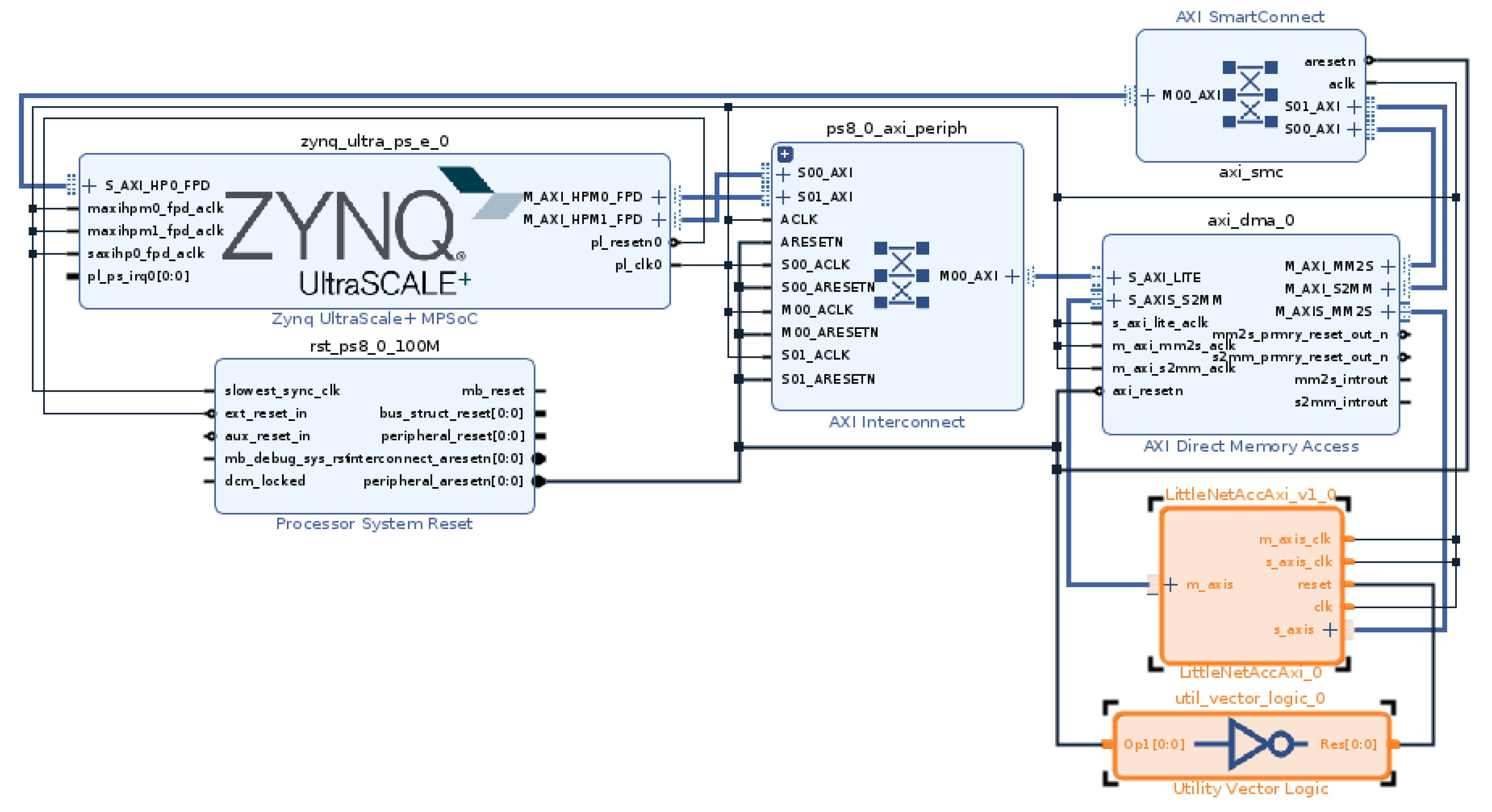
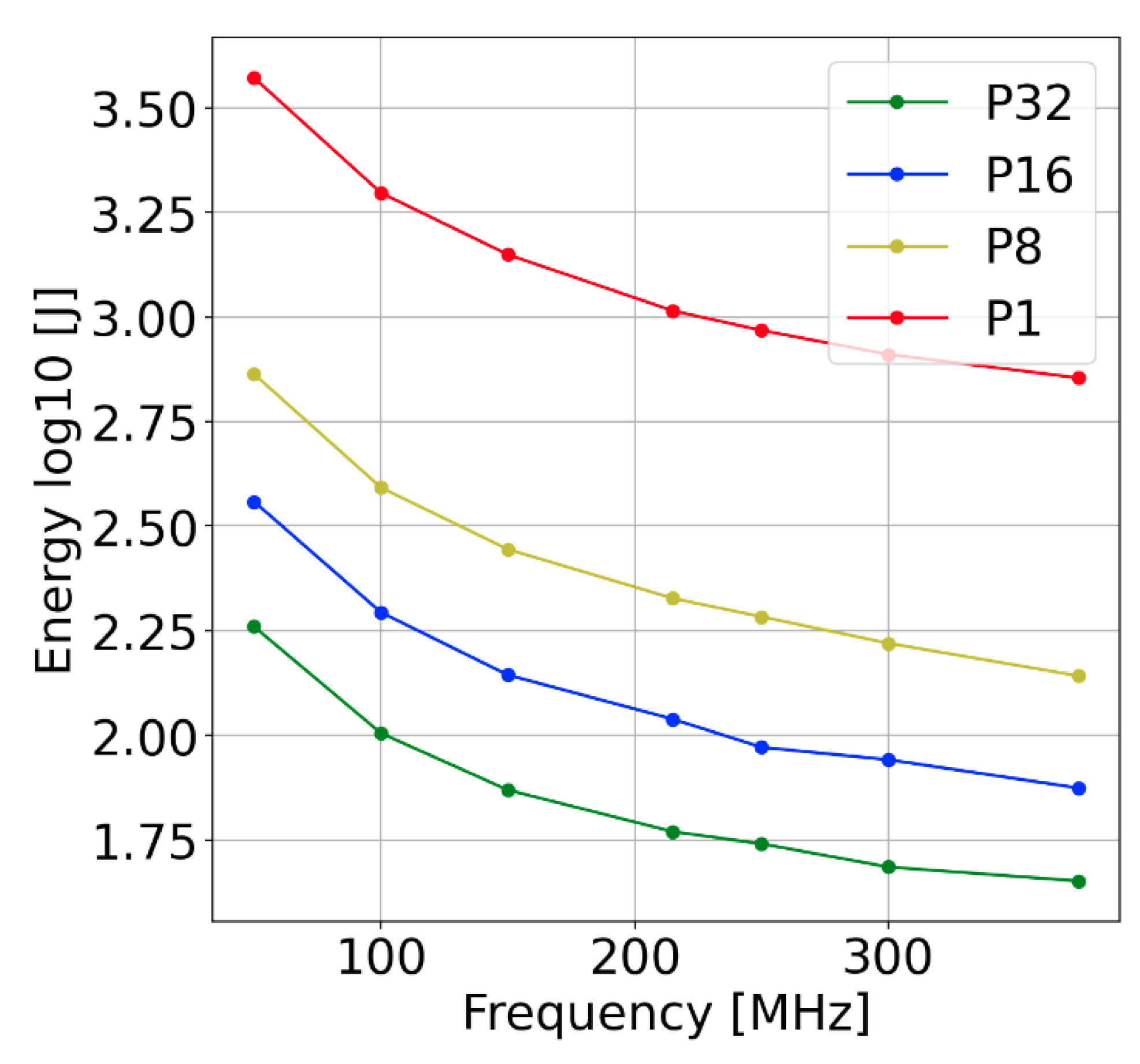
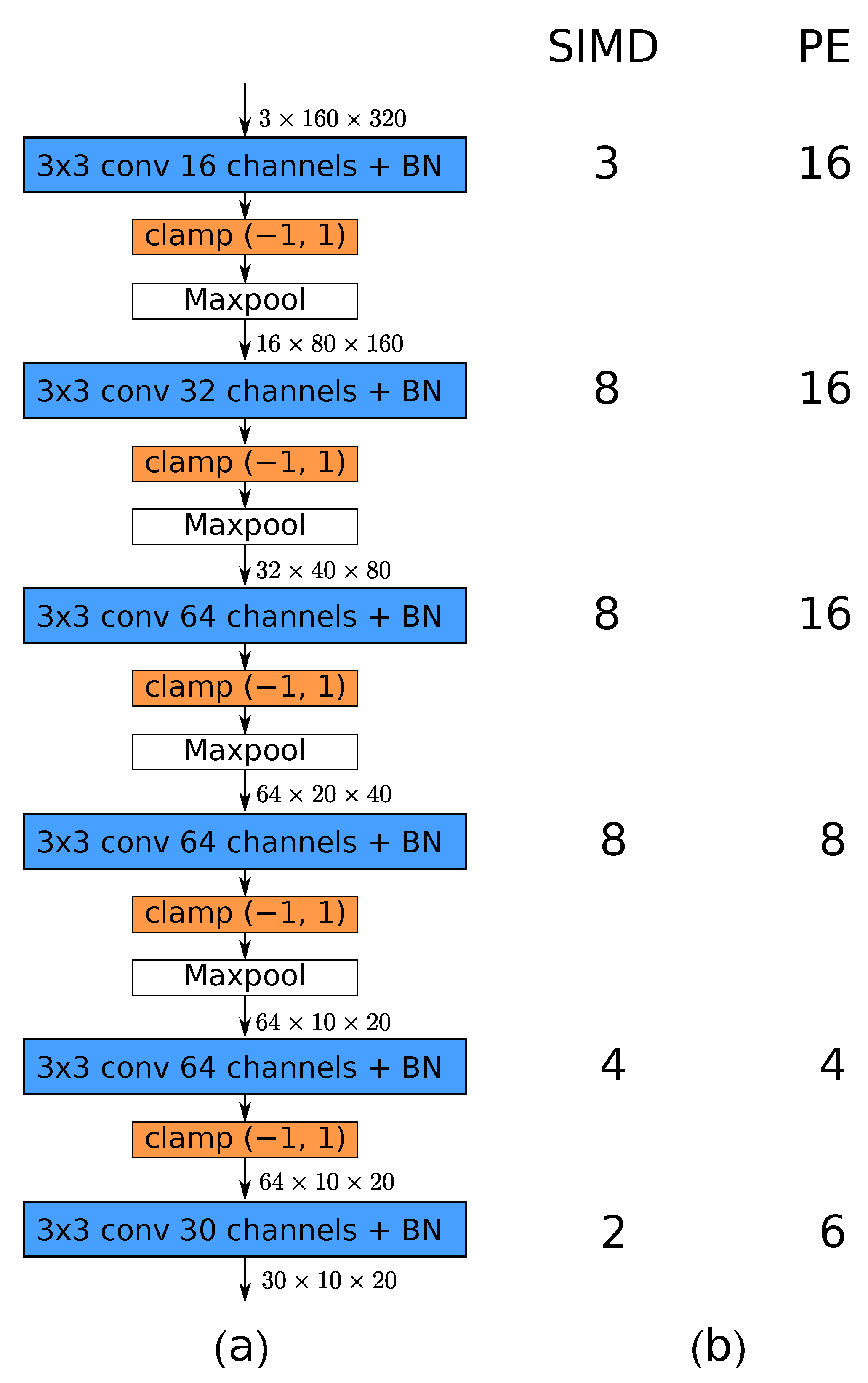
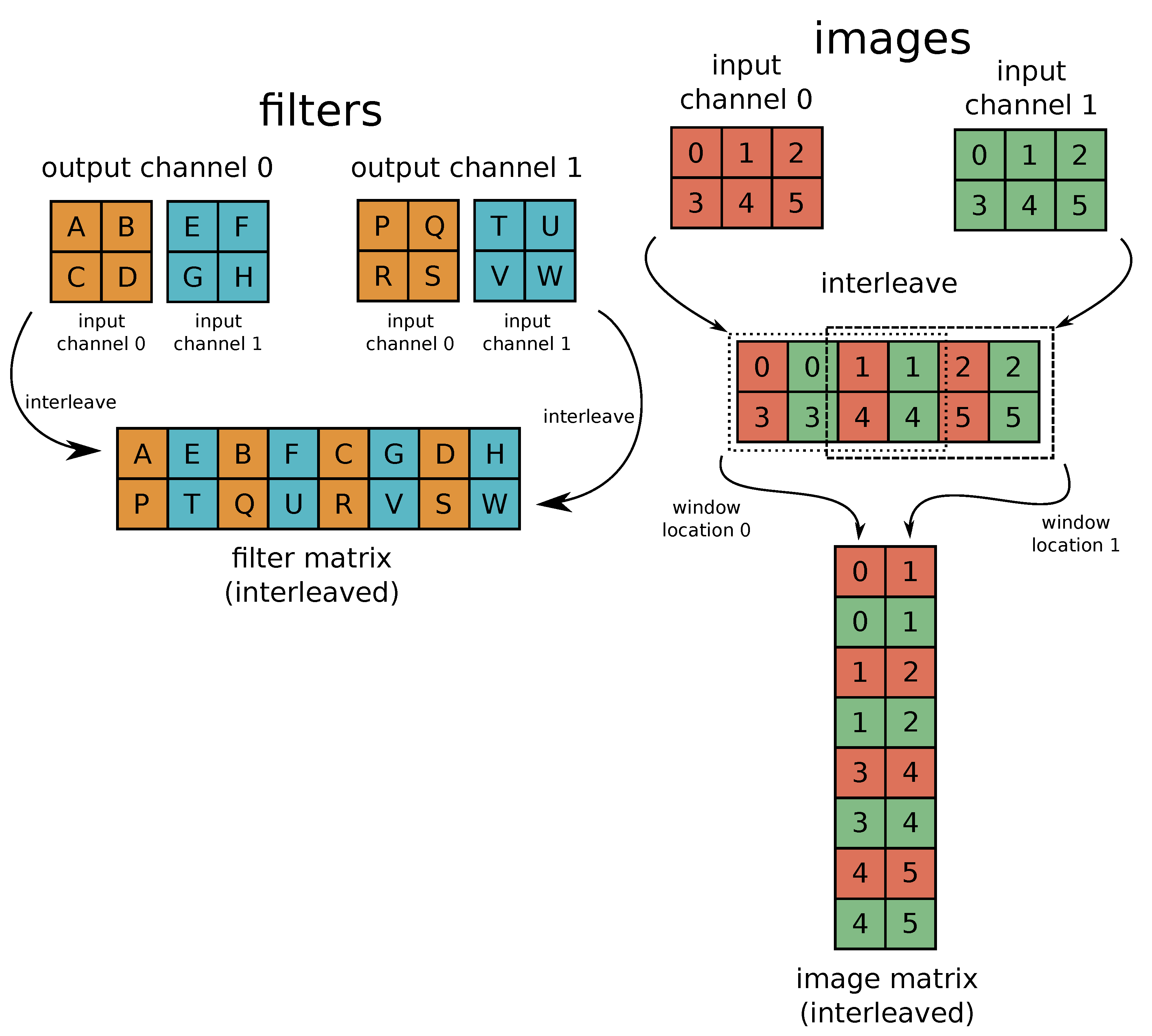
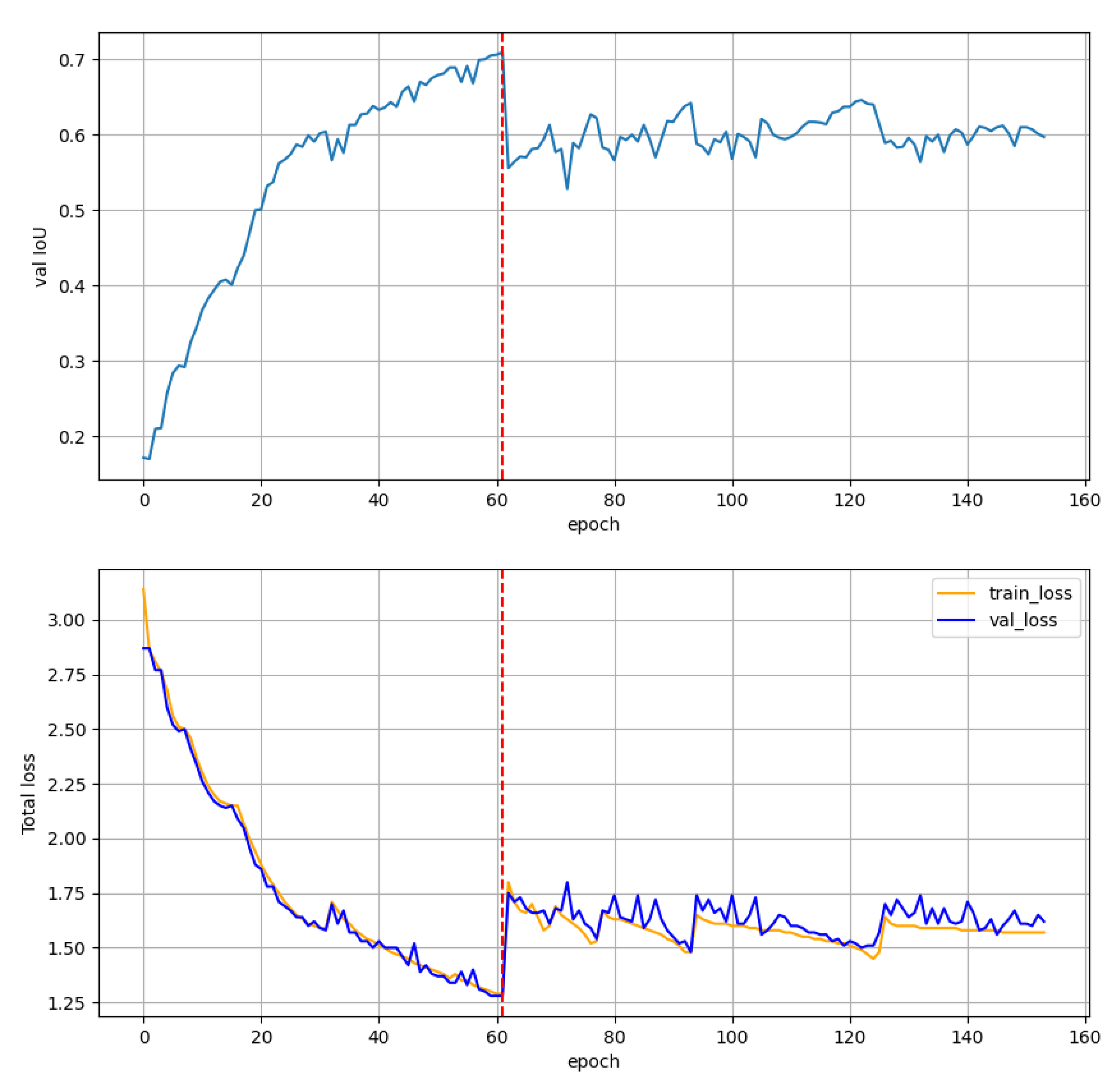
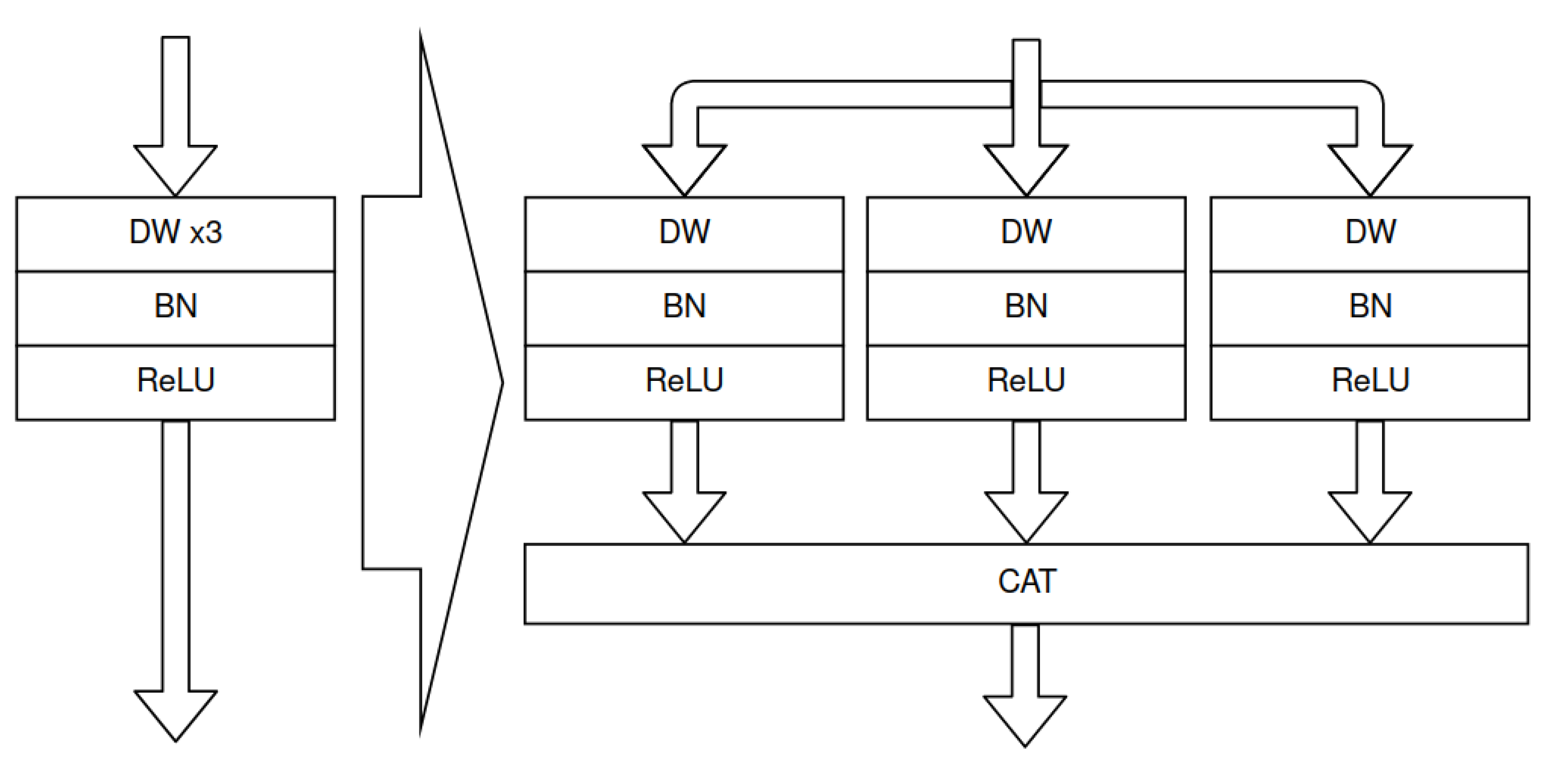
Table 1.
Applied parallelisation of pointwise accelerators.
| Layer | 2. PW | 5. PW | 8. PW | 11. PW | 14. PW | 17. PW | 19. PW |
| Parallelisation | 8 | 16 | 18 | 18 | 22 | 32 | 2 |
Table 2.
Normalised approximated times of execution. They were determined based on the multiplication of the input features maps’ sizes and the number of readings of the whole map. The weights reloading or initialisation times were ignored. The normalisation was performed by dividing all results by their largest value. The processing of PW layers takes much longer than DW layers.
| State | 0 | 1 | 2 | 3 | |
|---|---|---|---|---|---|
| Macroblock | |||||
| 0 | IL 0.0015 | DW 0.0117 | PW 0.0938 | DW 0.0039 | |
| 1 | DW 0.0078 | PW 0.2500 | DW 0.0039 | DW 0.0078 | |
| 2 | PW 0.5000 | DW 0.0020 | DW 0.0039 | PW 0.5000 | |
| 3 | DW 0.0010 | DW 0.0020 | PW 0.5000 | DW 0.0020 | |
| 4 | DW 0.0039 | PW 1.0000 | DW 0.0020 | PW 0.0312 | |
| 5 | MF 0.0001 | OL 0.0000 | |||
Table 3.
Maximal times of processing for each state for selected layer types. The duration of each state depends on the processing times of the PW layers.
Table 3.
Maximal times of processing for each state for selected layer types. The duration of each state depends on the processing times of the PW layers.
| State | 0 | 1 | 2 | 3 | Sum | |
|---|---|---|---|---|---|---|
| Layer Type | ||||||
| PW | 0.5000 | 1.0000 | 0.5000 | 0.5000 | 2.500 | |
| non-PW | 0.0078 | 0.0117 | 0.0039 | 0.0078 | 0.0312 | |
| all | 0.5000 | 1.0000 | 0.5000 | 0.5000 | 2.500 | |
Table 4.
Sets of parallelisation with labels. Configuration P32 allows for maximal performance. The next two have two and four times smaller parallelisms. The last one is the minimal configuration.
Table 4.
Sets of parallelisation with labels. Configuration P32 allows for maximal performance. The next two have two and four times smaller parallelisms. The last one is the minimal configuration.
| Layer | 2. PW | 5. PW | 8. PW | 11. PW | 14. PW | 17. PW | 19. PW | |
|---|---|---|---|---|---|---|---|---|
| Label | ||||||||
| P32 | 8 | 16 | 18 | 18 | 22 | 32 | 2 | |
| P16 | 4 | 8 | 9 | 9 | 11 | 16 | 1 | |
| P8 | 2 | 4 | 4 | 4 | 5 | 8 | 1 | |
| P1 | 1 | 1 | 1 | 1 | 1 | 1 | 1 | |
Table 5.
Evaluation results—energy consumptions and fps for different parallelisations and frequencies. There is a noticeable decrease in energy consumption for higher parallelisations and higher frequencies—for higher throughput in general.
Table 5.
Evaluation results—energy consumptions and fps for different parallelisations and frequencies. There is a noticeable decrease in energy consumption for higher parallelisations and higher frequencies—for higher throughput in general.
| Label | Frequency 1 [MHz] | Throughput [fps] | Energy [J] | Power [W] |
|---|---|---|---|---|
| P32 | 375 | 236 | 44.845 | 3.528 |
| 300 | 195 | 48.414 | 3.147 | |
| 250 | 167 | 55.032 | 3.063 | |
| 215 | 145 | 58.829 | 2.843 | |
| 150 | 105 | 73.990 | 2.590 | |
| 100 | 71 | 101.134 | 2.394 | |
| 50 | 35 | 181.750 | 2.120 | |
| P16 | 375 | 130 | 74.805 | 3.242 |
| 300 | 105 | 87.393 | 3.059 | |
| 250 | 88 | 93.597 | 2.746 | |
| 215 | 76 | 109.306 | 2.769 | |
| 150 | 53 | 139.347 | 2.462 | |
| 100 | 35 | 196.697 | 2.295 | |
| 50 | 17 | 361.815 | 2.050 | |
| P8 | 375 | 65 | 138.635 | 3.004 |
| 300 | 52 | 165.928 | 2.876 | |
| 250 | 43 | 191.968 | 2.752 | |
| 215 | 37 | 212.532 | 2.621 | |
| 150 | 26 | 278.281 | 2.412 | |
| 100 | 17 | 390.941 | 2.215 | |
| 50 | 8 | 729.939 | 2.115 | |
| P1 | 375 | 12 | 714.737 | 2.859 |
| 300 | 10 | 813.676 | 2.712 | |
| 250 | 8 | 928.440 | 2.476 | |
| 215 | 7 | 1034.701 | 2.414 | |
| 150 | 5 | 1409.458 | 2.349 | |
| 100 | 3.3 | 1979.160 | 2.177 | |
| 50 | 1.7 | 3727.046 | 2.112 |
1 For 375MHz, results of accelerator are non-deterministic. We included this frequency to check optimisation rules only.
Table 6.
Comparison of detection quality and resource utilisation for different degrees of quantisation.
Table 6.
Comparison of detection quality and resource utilisation for different degrees of quantisation.
| Precision | LUT Utilisation (% of Available) | IoU on Hardware Test Set |
|---|---|---|
| 8-bit | 301,968 (428%) | 0.7153 |
| 5-bit | 85,932 (122%) | 0.6970 |
| 4-bit | 54,079 (77%) | 0.6513 |
Table 7.
Evaluation results of acceleration with Vitis AI. Both models achieves similar accuracy, but with different throughputs and energy consumptions. The YoloFINN network has higher computational complexity, especially due to the applied activation approximation.
Table 7.
Evaluation results of acceleration with Vitis AI. Both models achieves similar accuracy, but with different throughputs and energy consumptions. The YoloFINN network has higher computational complexity, especially due to the applied activation approximation.
| Model | IoU | fps | Energy [J] | Power [W] |
|---|---|---|---|---|
| LittleNet | 0.6625 | 123.3 | 68.332 | 2.808 |
| YoloFINN | 0.6746 | 53.2 | 175.818 | 3.118 |
Table 8.
Results of acceleration with different methods. Abbreviations: C-G—coarse-grained, F-G— fine-grained, Seq.—sequential. The highest throughput is achieved by our C-G solution. YoloFINN architecture gives better accuracy results, but with higher computational complexity than LittleNet.
Table 8.
Results of acceleration with different methods. Abbreviations: C-G—coarse-grained, F-G— fine-grained, Seq.—sequential. The highest throughput is achieved by our C-G solution. YoloFINN architecture gives better accuracy results, but with higher computational complexity than LittleNet.
| Model | Method | Quantisation | fps | E [J] | P [W] | ||
|---|---|---|---|---|---|---|---|
| LittleNet | 0.6682 | C-G | 8-bit | 0.6616 | 196 | 49.88 | 3.259 |
| Seq. | 8-bit | 0.6625 | 123.3 | 68.33 | 2.808 | ||
| YoloFINN | 0.7209 | F-G | 4-bit | 0.6608 | 111 | 79.83 | 2.954 |
| Seq. | 8-bit | 0.6746 | 53.2 | 175.82 | 3.118 |
Table 9.
Resource usage for each architecture. Our coarse-grained solution can be considered as memory-hungry. On the other hand, the implementation with FINN uses more LUTs than other resources. Vitis AI DPU consumes less resources than our solution, but more than FINN.
Table 9.
Resource usage for each architecture. Our coarse-grained solution can be considered as memory-hungry. On the other hand, the implementation with FINN uses more LUTs than other resources. Vitis AI DPU consumes less resources than our solution, but more than FINN.
| HW Architecture | LUT | LUT RAM | FF | BRAM | DSP |
|---|---|---|---|---|---|
| LN P32 | 33,029 | 7077 | 64,918 | 198.5 | 349 |
| LN P16 | 25,321 | 4724 | 47,339 | 198.5 | 238 |
| LN P8 | 21,025 | 3772 | 39,328 | 202.5 | 187 |
| LN P1 | 17,120 | 3044 | 30,023 | 205.0 | 140 |
| Vitis AI DPU 1 | 45,051 | 0 | 63,033 | 168.0 | 262 |
| Vitis AI DPU 2 | 34,924 | 2875 | 57,094 | 163.0 | 312 |
| YoloFINN 4-bit | 54,079 | 8002 | 57,118 | 26.5 | 10 |
1 Resource utilisation designated on the basis of documentation [38]; 2 Resource utilisation designated on the
basis of Vivado’s implementation reports.
Table 10.
Parameter numbers and characteristics of selected networks architectures.
| Network Architecture | Dataset | Parameters | Features |
|---|---|---|---|
| YOLOv3-tiny [39] | COCO | 8.818 M | multi-scale detection, standard convolutions, upsampling |
| MobileNetV2 [40] | COCO | 4.3 M | separable convolution, inverted residual blocks |
| SkyNet [20] | DAC SDC | 0.309 M | separable convolution, PSO algorithm used for structure optimisation |
| UltraNet [35] | DAC SDC | 0.256 M | , standard convolution with quantisation |
| LittleNet (our) | VOT+VTB | 0.244 M | multi-depthwise convolution, linear activation for some layers, anchors multipliers |
| YoloFINN (our) | VOT+VTB | 0.115 M | activation function |
Publisher’s Note: MDPI stays neutral with regard to jurisdictional claims in published maps and institutional affiliations. |
© 2022 by the authors. Licensee MDPI, Basel, Switzerland. This article is an open access article distributed under the terms and conditions of the Creative Commons Attribution (CC BY) license (https://creativecommons.org/licenses/by/4.0/).
Share and Cite
MDPI and ACS Style
Machura, M.; Danilowicz, M.; Kryjak, T. Embedded Object Detection with Custom LittleNet, FINN and Vitis AI DCNN Accelerators. J. Low Power Electron. Appl. 2022, 12, 30. https://0-doi-org.brum.beds.ac.uk/10.3390/jlpea12020030
AMA Style
Machura M, Danilowicz M, Kryjak T. Embedded Object Detection with Custom LittleNet, FINN and Vitis AI DCNN Accelerators. Journal of Low Power Electronics and Applications. 2022; 12(2):30. https://0-doi-org.brum.beds.ac.uk/10.3390/jlpea12020030
Chicago/Turabian StyleMachura, Michal, Michal Danilowicz, and Tomasz Kryjak. 2022. "Embedded Object Detection with Custom LittleNet, FINN and Vitis AI DCNN Accelerators" Journal of Low Power Electronics and Applications 12, no. 2: 30. https://0-doi-org.brum.beds.ac.uk/10.3390/jlpea12020030
Note that from the first issue of 2016, this journal uses article numbers instead of page numbers. See further details here.