Article

Path Planning for Highly Automated Driving on Embedded GPUs

1
Hardware/Software Co-Design, Department of Computer Science, Friedrich-Alexander University Erlangen-Nürnberg (FAU), 91054 Erlangen, Germany
2
GIGATRONIK Ingolstadt GmbH, Ingolstadt, 85080 Gaimersheim, Germany
3
Pre-/Concept Development Automated Driving, AUDI AG, 85045 Ingolstadt, Germany
*
Author to whom correspondence should be addressed.
J. Low Power Electron. Appl. 2018, 8(4), 35; https://0-doi-org.brum.beds.ac.uk/10.3390/jlpea8040035
Submission received: 24 August 2018 / Revised: 21 September 2018 / Accepted: 28 September 2018 / Published: 2 October 2018
(This article belongs to the Special Issue Automotive Low Power Technologies)

Abstract

:
The sector of autonomous driving gains more and more importance for the car makers. A key enabler of such systems is the planning of the path the vehicle should take, but it can be very computationally burdensome finding a good one. Here, new architectures in Electronic Control Units (ECUs) are required, such as Graphics Processing Units (GPUs), because standard processors struggle to provide enough computing power. In this work, we present a novel parallelization of a path planning algorithm. We show how many paths can be reasonably planned under real-time requirements and how they can be rated. As an evaluation platform, an Nvidia Jetson board equipped with a Tegra K1 System-on-Chip (SoC) was used, whose GPU is also employed in the zFAS ECU of the AUDI AG.

1. Introduction and Related Work

1.1. Motivation

In the automotive industry, the sector for Advanced Driver Assistance Systems (ADASs) has enormously grown over the last years, and the most significant growth is still to come, with the moving to more and more autonomy. Nowadays, driver assistance systems, such as adaptive cruise control, parking assist, or lane-keeping assistance systems are available. However, the driver must permanently monitor the behavior of the vehicle and, in case of malfunction, intervene. In the future, fully responsible systems, so-called highly and fully automated systems, will be available for all driving-related tasks. These will reshape mobility completely, e.g., by enhancing safety and comfort or introducing new transportation concepts, such as robot taxis. One primary task in such systems is the planning of the path, which determines the path being taken by the vehicle. In the real world, for a dependable, highly and fully automated driving vehicle, a multitude of paths has to be considered and evaluated to ensure that the chosen way is safe, comfortable, and a dynamically possible path. However, today’s standard processors in ECUs struggle to provide enough computing power for the enormous computational complexity, due to their lack of parallel computation capacities. As a remedy, we propose to substitute Central Processing Units (CPUs), responsible for path planning, with GPUs, embodying hundreds of cores, even as embedded versions. In this work, we introduce a highly efficient path planning algorithm for GPUs, based on quintic polynomials. Our approach targets highway scenarios and is for SAE Level 2 or above [1]. At these levels, the system has the control of the vehicle in lateral and in longitudinal direction. In addition, we show how many paths can be planned reasonably under real-time requirements and where the sweet spot of the proposed algorithm on a GPU and CPU architecture is.
The remainder of the paper is structured as follows: In the next paragraph, we discuss the differences of our approach compared to related work. In Section 2, the fundamentals and the parallelization of our path planning algorithm are described. In Section 3, experimental results of our approach are presented and discussed. Finally, we conclude the paper in Section 4.

1.2. Related Work

Path planning has its origin in robotics. Here, the ultimate goal is [2] to create an autonomous robot, where user input is transformed, without further interventions, in the right motions of the robot to achieve the desired task. Quite a lot of research has been done in the area of path planning algorithms for robotics, so already several algorithms, such as sampling or roadmap based [3], exist. Some were adapted to the automotive sector, where a distinction can be made between approaches, which plan paths for structured and dynamic environments [4,5] and for unstructured, but mostly static environments [6,7]. Generally, it can be distinguished between several approaches of how to plan the vehicle’s path. Some methods are based on a discrete state grid [4,8]. Paths planned with these methods can be computed efficiently, but lack in accuracy. Another approach is the optimization of kinematic quantities [9,10]. These methods are based on a mass point model and minimize kinematic or geometric sizes. In August 2013, Mercedes Benz used this approach during the Berta Benz drive, were a mostly autonomous vehicle drove the Bertha Benz Memorial Route [11]. Furthermore, there are model predictive procedures [12,13]. They integrate dynamic models into the planning to make them more accurate and to ensure the feasibility of the path. A completely different approach to solving the path planning problem is multi-agent systems, where the necessary calculations are distributed among different units [14]. Most of the path planning approaches plan several paths, evaluate these and choose the best [5,15], but there are also approaches, which plan only one path and iteratively improve this path [16]. Because path planning can become computationally burdensome, a considerable amount of research was done to parallelize it. Burns et al. [17] presented a parallel CPU approach with up to eight threads. In [18], an A * algorithm for path planning is parallelized on a GPU, but only a speedup of two, compared to a single-threaded CPU version could be achieved. Kider et al. [19] achieved much higher speedups, by using an improved A * algorithm, the so-called R * algorithm. The above-mentioned parallel approaches were introduced in the field of robotics. In [20], a swarm intelligence method is parallelized on a desktop GPU and used for path planning of an unmanned airborne vehicle. McNaughton et. al. [4] presented a motion planning approach, based on conformal spatiotemporal lattice and parallelized it on a desktop GPU. In [21], a path planning algorithm for an unmanned airborne vehicle is analyzed, but they did their experiments on an embedded GPU, as we do in our work. Contrary to their approach, ours is based on quintic polynomials, as in the work of [5]. The difference to [5] is that, one the one hand, the planned paths are evaluated with a different function, which considers more parameters, and, furthermore, the rating points of the paths are included in the evaluation of the paths. In [5], only the endpoints of the planned paths are evaluated. On the other hand, we evaluated the approach for a different number of rating points and paths, which has also not been evaluated in the other work. To the best of our knowledge, this is the first time that such an approach was parallelized for an embedded GPU in the automotive context. The advantage of our approach is that an optimal solution, within the discretized space, is found in a certain deterministic time. The space is discretized by the number of planned paths. The higher the number of planned path is, the smaller is the discretization. Instead, with A * approaches, there is mostly a solution in less time, but there is no guarantee that you will find an optimal solution within a certain time. For safety-critical applications (SAE Level 3), however, it is essential for security reasons to find a solution in a certain time.

2. Methods

2.1. Programming an Embedded GPU

GPUs have initially been introduced for image processing, or rather for graphics output from desktop computers. With their large number of specialized cores that run into the thousands for desktop GPUs and hundreds for embedded GPUs, they are far superior to CPUs in problems designed for such architectures. Not only the architectures differ between CPUs and GPUs, but also the programming models. On a CPU, the programming model is Multiple Instruction, Multiple Data (MIMD), while, on a GPU, the programming model is Single Instruction Multiple Thread (SIMT). This means that on a CPU, parallelized programs perform different operations on different data at the same time, whereas on a GPU all threads perform the same instructions on different data at the same time. In 2006, Nvidia introduced the CUDA framework [22], which facilitates General-Purpose Computation on Graphics Processing Unit (GPGPU) on Nvidia GPUs. Now, it was more practical to accelerate compute-intensive problems from various domains, besides the classical image processing, such as financial services [23], SQL Database Operations [24], etc. Generally, program blocks that should be executed in parallel are called kernels in CUDA. A kernel is similar to a function in C. Each kernel is executed by n threads specified by the programmer. The threads are grouped in so-called warps on the GPU, which contain 32 threads. Each thread in a warp executes the same instruction at the same time. In CUDA threads are grouped into logical blocks and blocks are grouped into logical grids, as illustrated in Figure 1. The programmer can specify the size, the dimensions (1D,2D,3D) and numbers of these structures. At the hardware level, the GPU has one or more streaming processors, which itself contain several executing units. The blocks are executed on the GPU by streaming processors, with each block allocated exactly one streaming processor. The major difference between a desktop GPU and an embedded GPU is that the memory of the desktop GPU is separated from the system memory. Instead, for an embedded GPU, the system memory and the memory of the GPU are the same, as illustrated in Figure 1. Therefore, it is not necessary to explicitly copy the data to the GPU and copy the results back into the system memory. The Nvidia Jetson K1 platform, which was used for the evaluation of our algorithm, is such an embedded GPU.

2.2. Overview

Generally, between two major steps in path planning, algorithms can be distinguished: the rough planning and the detailed planning. In rough planning, the possible solution space for the detailed planning is reduced, by examination where the vehicle is allowed to drive, e.g., no obstacle on an endpoint of a path. The endpoint of a path is the temporary target position of the vehicle. Furthermore, the reference path is determined during rough planning. In Figure 2, the dashed orange lines, which are parallel to the reference path, illustrate possibilities for endpoints of paths. The blue points are concrete calculated endpoints, nine in this case. The paths are planned from the vehicle to these points. During detailed planning, which is evaluated for parallelization in this paper, the single paths are completely planned, evaluated, and, finally, the best one is chosen. Our parallelized path planning algorithm is based on Werling et al. [5,25], who used quintic polynomials for generating the lateral as well the longitudinal part of the paths. The new path is calculated based on the relative position to the reference path. The goal is to lead the vehicle on a path between the two corridor boundaries, respectively driving tube. Since it is assumed that the vehicle is always driven in a structured environment, there are road or lane edges, respectively markings, and therefore the reference path can be set into the middle of one lane. The detailed path planning, as also illustrated in Figure 2, consists of the following steps:
  • Calculate start values in Frenet coordinates for the path planning algorithm in relation to the current vehicle position.
  • Plan different paths with different lengthwise and crosswise variations with respect to the reference path.
  • Transform from Frenet coordinates to Cartesian coordinates.
  • Calculate the costs for each path and select the best path.

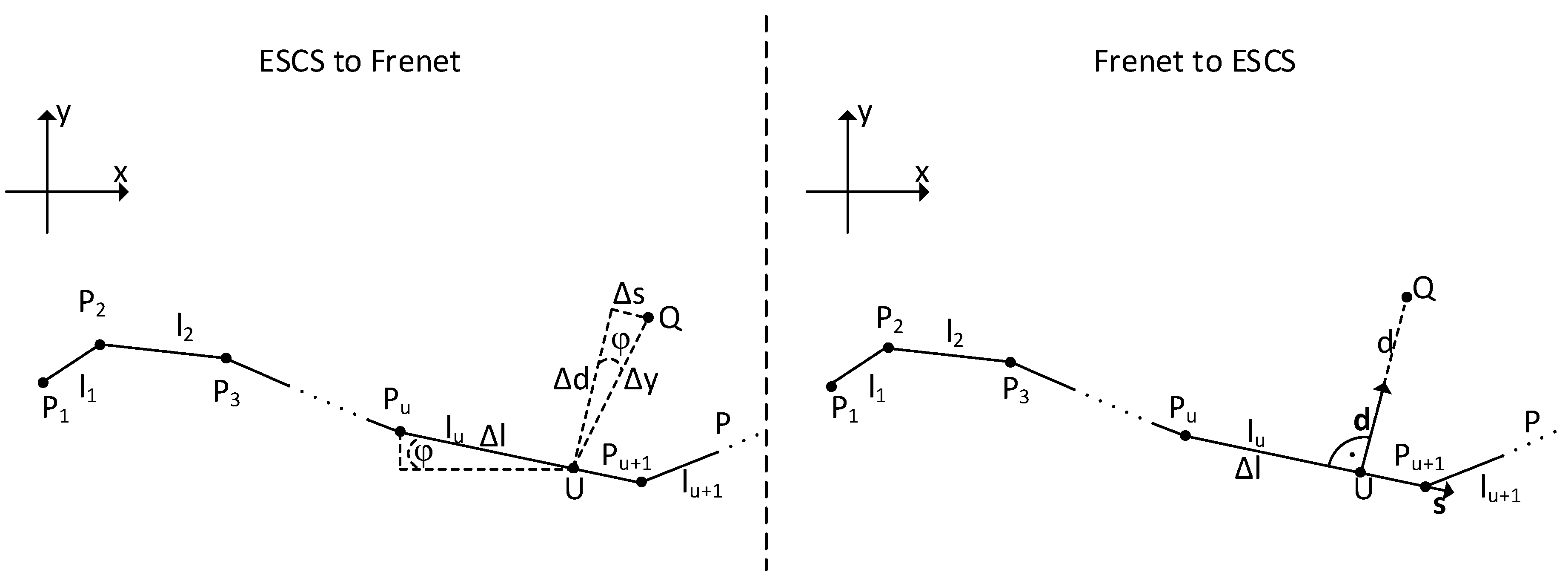
2.3. Frenet Coordinates

The Frenet coordinates [26], also known as the Frenet–Serret formulas, describe the geometric properties of a curve. Let r ( t ) be a curve in three-dimensional Euclidean space R 3 , which represents the position vector of a particle as a function of time t and l ( t ) the arc length, which a particle has moved along the curve in time t. r ˙ ( t ) is the velocity of the particle, and r ¨ ( t ) the acceleration. It is assumed that r ˙ 0 and therefore l is a strictly monotonically increasing function. Then, it is possible to solve for t as a function of l and it can be written r ( l ) = r ( t ( l ) ) . The coordinate system is formed by s , d , and b . It is defined in R 3 , but it is also possible to generalize it for higher dimensions, as follows:
  • s is the tangent unit vector, s = d r d l d r d l
  • d is the normal unit vector, d = d s d l d s d l
  • b is the binormal unit vector, b = s × d
The Frenet–Serret formulas, stated in a skew-symmetric matrix [27], are:
s d b = 0 κ 0 κ 0 τ 0 τ 0 s d b
where κ is the curvature and τ is the torsion of the curve.
For the path planning algorithm, it is not necessary to know the absolute coordinates of the planned path. Having coordinates relative to the vehicle’s position is sufficient. In our case, s indicates how far the vehicle has moved along the path and d is the distance of the normal to the observed point. Therefore, the Frenet coordinate system indicates the distance of a point to the reference path, from the position of the own vehicle. The usage of Frenet coordinates uncurls the coordinate system and allows the separated optimization of lengthwise and crosswise path planning, respectively. In each planning step, the start state described in the Environment Sensor Coordinate System (ESCS) is transformed into the Frenet space in order to calculate then a path to the target point also described in Frenet space. The result is then transformed back into the ESCS. Since the computational effort for the coordinate transformation is quite high, some approximations are used to reduce this effort. To get the Frenet coordinates s and d of a point Q, the following limitations apply:
  • The change of the angle between two polygon courses can only be moderate. Otherwise, there will be jump discontinuity in the polygon course. Since our approach is proposed for highway scenarios, that is not a limitation.
  • The polygon course has to be monotonically increasing along the x-axis.
  • The path P is an open polygon course and is defined as P = { P 1 P 2 , , P n } with S 1 = [ P 1 , P 2 ] , S 2 = [ P 2 , P 3 ] , , S n 1 = [ P n 1 , P n ] .
In Figure 3, the coordinate transformation from Cartesian coordinates (ESCS) to Frenet coordinates, as well as the other way round are illustrated. On the left side, the Frenet coordinates for a given point Q in the ESCS are computed. On the right side of Figure 3 a point Q is given in Frenet Coordinates and the corresponding ESCS coordinates should be determined. The ESCS’ origin is in the middle of the vehicle’s rear axis. To obtain s, it is first necessary to calculate an auxiliary point U, which is the intersection point of path P with a parallel line to the y-axis through the point Q. The segment on which the point U lies is S t . The length of one segment S i is l i . The partial length l is the length of the segment S ^ = [ B u U ] . With the limitations mentioned above, s results from the sum of all lengths l i of the sections which lie before a point U, the partial length l and the correction term s .
s = i = 1 u 1 l i + l + s with s = y · sin φ
The correction term s = y · sin φ is necessary and improves the approximation, if the segment S u is not parallel to the x-axis. It is calculated from the vertical distance y of point Q to the path P and the rotation ϕ around the segment S u , which is rotated with respect to the x-axis. The calculation of d follows the same procedure:
d = d = y · cos φ
After the paths are planned in Frenet coordinates, it is necessary to transform them back into the ESCS. Therefore, the Frenet coordinates s and d, respectively, the longitudinal and lateral portion, should be transformed to x and y coordinates in the ESCS. They refer to the path P, which will be covered by an open polygon ( P 1 , P 2 , , P n ) with the lines ( S 1 = [ P 1 P 2 ] , S 2 = [ P 2 P 3 ] , , S n = [ P n 1 P n ] ) . s in Frenet coordinates is equal to a distance between the searched point U and the start point B u . Therefore, s is:
s = i = 1 u 1 l i + l
If U is calculated, it is possible to determine the normal vector d on the segment S u . Afterwards, d has to be extended to the length d to get the point Q:
Q = U + d · d
Due to the independence of the rating points of each path and also the independence between the different paths, it is possible to create one CUDA thread for every rating point of each path. Thus, one CUDA thread transforms one point Q from ESCS to Frenet coordinates s and d or vice versa.

2.4. Path Generation

To generate a single path, it is necessary to find a continuous course ξ ( t ) , which transfer the initial state ξ ( 0 ) into the final state ξ ( τ ) [5]. To calculate the continuous course ξ ( t ) , the following equation has to be solved:
ξ ( t ) = M 1 ( t ) c 012 + M 2 ( t ) c 345 with t [ 0 , τ ] with τ > 0 and τ = { τ s , τ d }
This course can be computed by determining the coefficients of a fifth-degree polynomial c 012 T , c 345 T = c 0 , c 1 , c 2 , c 3 , c 4 , c 5 , c 6 . The coefficient c 012 is independent of the final state ξ ( τ ) and results from:
c 012 = M 1 ( 0 ) 1 ξ ( 0 ) with M 1 ( t ) = 1 t t 2 0 1 2 t 0 0 2 and M 1 ( 0 ) 1 = 1 0 0 0 1 0 0 0 0.5
The other coefficient c 345 results from:
c 345 = M 2 ( τ ) 1 ξ ( τ ) M 1 ( τ ) c 012 with M 2 ( t ) = t 3 t 4 t 5 3 t 2 4 t 3 5 t 4 6 t 12 t 2 20 t 3 and M 2 ( τ ) 1 = 1 2 t 5 20 t 2 8 t 3 t 4 30 t 14 t 2 2 t 3 12 6 t t 2
In literature, a path, which has information of how to traverse it with respect to time, e.g., a velocity profile is also called trajectory. In this paper, we use the term path for simplicity synonymously. For an autonomous vehicle, it is not sufficient to plan only a single path. For such cars, a lot of paths have to be planned and evaluated to find one, which fulfills the requirements of safety and comfort. Every path has the same initial state lengthwise s 0 and crosswise d 0 , which is the current state of the vehicle. Only the final states lengthwise s τ and crosswise d τ are varied. Thereby, s τ is varied in time and d τ by distance. The variation of these two components, which make up an endpoint of a path, results in a multitude of variations. Every state has three components: s is the lengthwise relative position, s ˙ ( t ) the velocity, and s ¨ the acceleration. The same applies to d. Therefore, we have:
ξ s ( t ) = s ( t ) s ˙ ( t ) s ¨ ( t ) and ξ d ( t ) = d ( t ) d ˙ ( t ) d ¨ ( t )
For the computation of the lengthwise part, the same algorithm is used as for the crosswise part, but they are executed in succession. Since it is mathematically burdensome to calculate the continuous course ξ ( t ) for thousands of paths, they are predestined to be calculated on a GPU. At first, the lengthwise part of a path with associated rating points is computed. Due to the dependence between the lengthwise part of a path and the crosswise part of a path, the crosswise part, with associated rating points, has to be computed after the lengthwise part. On the contrary, the rating points of each path lengthwise as well crosswise are independent. Therefore, one CUDA thread can be started for each rating point of each path lengthwise and crosswise, respectively.
The part that the vehicle already traveled is deleted from the current path. Only if there is no valid path at all or the rest of the current path is too short, a new path is entirely planned from scratch.

2.5. Rating of Paths

After planning numerous paths, it is necessary to evaluate them, and to find the one which fulfills the requirements the most. Those requirements, amongst others, can be:
  • Distance to the left corridor boundary ( d c l ) and to the right corridor boundary ( d c r ).
  • A crosswise deviation related to the reference path in the endpoint of the path ( d R E F ).
  • Maximum lateral acceleration ( d a c c l Y ) of the vehicle along the planned path.
Therefore, the total costs C are in this case:
C = λ C · 1 ( d c l + d c r ) + λ R E F · d R E F + λ A · d a c c l Y with λ C + λ R E F + λ A y = 1
where λ C , λ R E F , and λ A y are weighting factors of the requirements. In the end, the path with the smallest cost is chosen. Therefore, for each path, its cost function C is calculated. In Figure 4, the evaluation of one path, which has two rating points, is illustrated.
Since every rating point of each path is independent, it makes sense to create one CUDA thread for every rating point, which calculates the cost function C. After C is calculated, the one with the lowest costs has to be chosen. This is done on the CPU. Solving this reduction problem on the GPU would not be rational because of the small number of operations necessary and, therefore, the small number of CUDA threads, which could be used. In addition, the results of the threads would have to be synchronized via shared memory on the GPU, which would require further computation time.
As mentioned above, an important criterion in the evaluation of a path P is the distance to the corridor boundaries. For each rating point, the Euclidean distance to the corridor boundaries is calculated. For the final cost calculation, only the smallest Euclidean distance of the path is taken, because it is vital to leave the corridor boundaries nowhere.

3. Experiments

3.1. Evaluation Environment

Our experimental platform is an Nvidia Jetson board [28]. The board embodies an embedded Nvidia Kepler GPU with 192 CUDA cores at 850 MHz. The CPU is a quad-core ARM Cortex-A15 with 2.3 GHz. Although the board has a high computing power, the energy consumption amounts only to 8–10 W, which results in a high performance per Watt ratio. With such a low energy consumption, it is possible to cool a board passively, which is essential for embedded systems in general and ECUs in cars in particular. First, we implemented a single-threaded reference implementation in the programming language C. Each C implementation is tested on one of the ARM cores available on the Jetson board. Thereby, we can show which algorithm could be potentially accelerated on the embedded GPU and which speedups are achievable. To smooth jitter in the experiments, all experiments are always performed 100 times, and the mean value is taken.

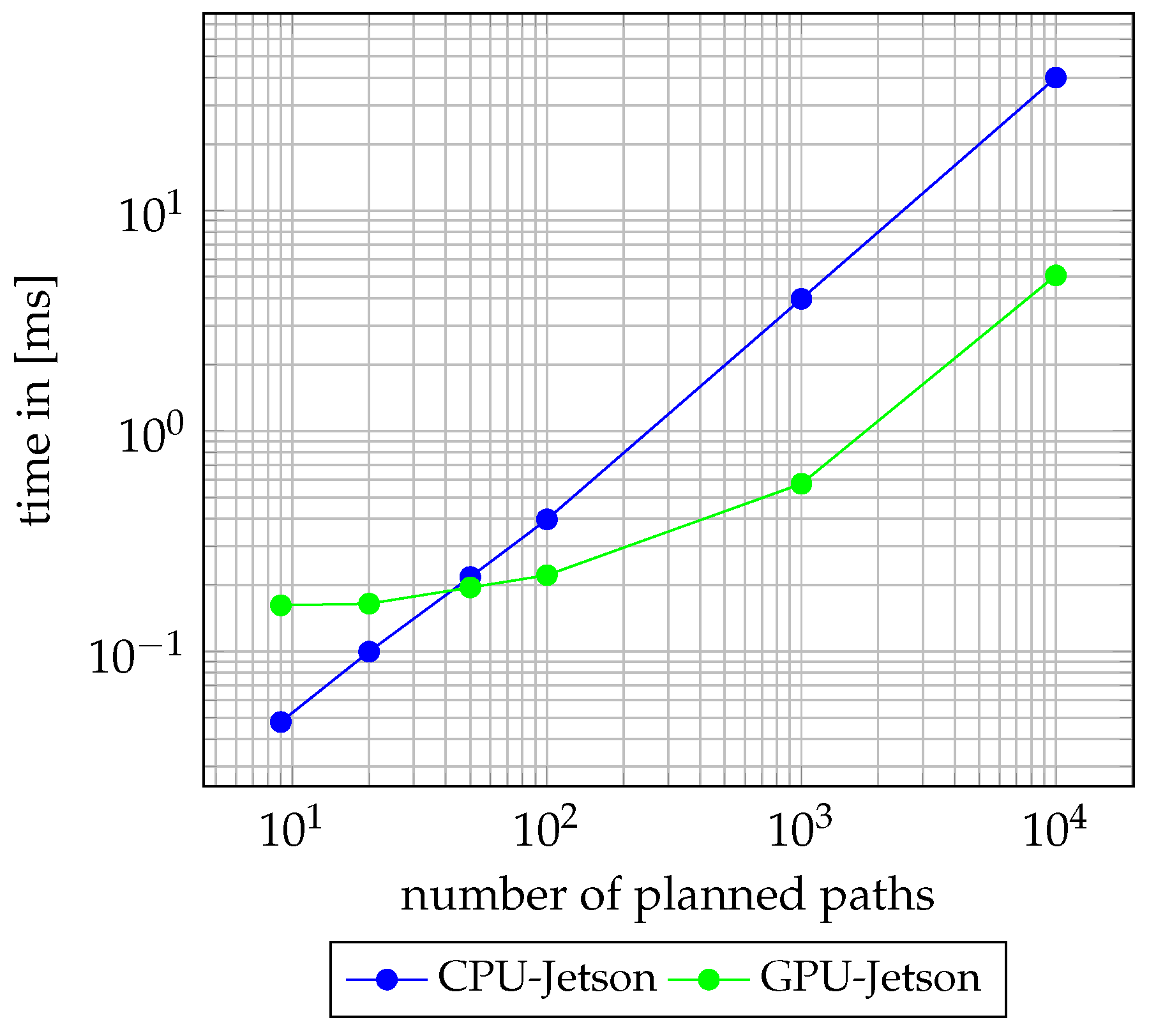
3.2. Evaluation of the Coordinate Transformation from Frenet Coordinates to Cartesian Coordinates

Since we plan our paths in Frenet coordinate space, but the final map coordinate system is in Cartesian space, a coordinate transformation is necessary. Therefore, all paths, including the rating points of each path, have to be transformed from Frenet into Cartesian coordinate space. At the first evaluation of the coordinate transformation, the number of paths was varied and a fixed number of rating points, 20 in this case, was chosen. As can be seen in Figure 5, the GPU outperforms the CPU nearly in all configurations. The reason for the high speedup is that the coordinate transformation can be parallelized straightforwardly because there are no data dependencies between the single rating points, as well between the individual paths. Only the configuration with the smallest number of paths the CPU is faster than the GPU. Here, the GPU cannot be fully exploited, to due to unbalanced and low workload in the warps. A warp consists of 32 threads, which is the smallest unit threads are grouped on an Nvidia GPU. Even if only 16 threads are active in a warp, resources for 32 might be allocated. The increase in computing time on the GPU is not linear, due to its low utilization for a small number of planned paths. In Figure 6, a plateau occurs for the evaluation of varying rating points on the GPU. This is due to a different number of blocks, in which the threads are grouped. With an increasing number of blocks, the workload can be scheduled better on the GPU’s streaming processors and almost no increase in execution time occurs. In addition, if the number of threads in a block is not multiple of 32, the GPU cannot be fully exploited. We also performed experiments, with an increased number of blocks for a low number of paths, but no decrease in execution time could be observed. Another reason is that the usage of a GPU has an overhead. The necessary area for the data must first be allocated, then the data which have to be processed need to be copied to that area and finally the results have to be copied back. This is particularly noticeable in the case of low-complexity problems and their execution time, such as a small number of paths or evaluation points. In the second experiment considering the coordinate transformation, the number of paths was set to nine and the number of rating points was varied. The number of paths was set to nine because, even if the number of rating points per path is increased, every step of the algorithm is executed once. For nine paths and endpoints, we have a variation of three in the longitudinal direction and then, for each of these points, a variation of three in the lateral direction.
The results of that experiment are illustrated in Figure 6. Similar to the previous experiment, the workload on the GPU is for a small number of rating points per path not high enough to fully utilize the GPU. With an increasing number of rating points, the speedup between the CPU and GPU increases, due to better utilization of the GPU. By comparing both experiments, it can be seen that for an increased number of paths, respectively rating points per path, the growth in execution time is similar.

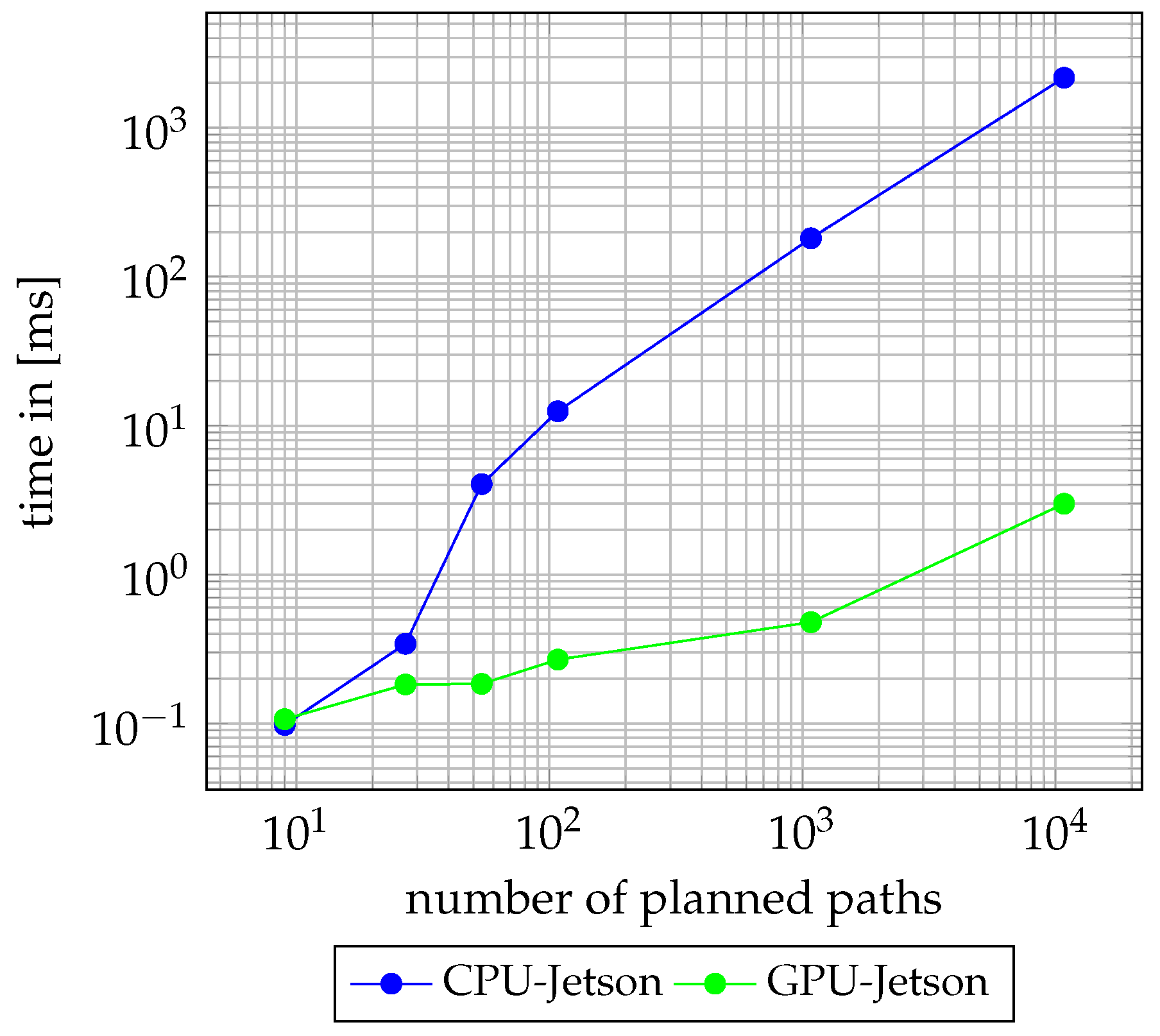
3.3. Evaluation of Lengthwise and Crosswise Path Planning

Our approach for path planning first solves the variational problem lengthwise and then crosswise. In the following experiment, the number of endpoints of the paths in the lengthwise and the crosswise direction were increased. In the first test case of this experiment, the entire number of planned paths was nine, a mesh of 3 × 3 endpoints. If the number of endpoints was increased, they were increased in lateral, as well in longitudinal direction, e.g., to 45, the mesh of endpoints had the size 9 × 5 , nine in the longitudinal and five in the lateral direction. In this experiment, the number of paths was varied whereas the number of rating points per path remained fixed.
As illustrated in Figure 7, the GPU outperforms the CPU already for a small number of paths, which is nine in this case. The reason is that it is quite mathematically complex to solve the variational problem in longitudinal as well as in lateral direction. The complexity of the path planning algorithm is O ( m · n · o ) , with m the number of endpoints in longitudinal direction, n the number of endpoints in lateral direction and o the number of rating points per path. Typically, both m and n are increased. With an increasing number of rating points per path, the speedup between the GPU and CPU also increases. We also evaluated the solution of the variational problem lengthwise and crosswise, separately. In general, the execution times were lower due to the less number of paths planned and also the break-even point is starting later, i.e., where the GPU outperforms the CPU.
In the following evaluation, the number of rating points per path was varied, whereas the number of paths remained the same. The results of that experiment are shown in Figure 8. Similar to the previous experiment, the GPU outperforms the CPU for all scenarios. The calculation of numerous rating points for each path also requires numerous mathematical operations, which is the reason that the GPU is already faster than the CPU for a small number of rating points.

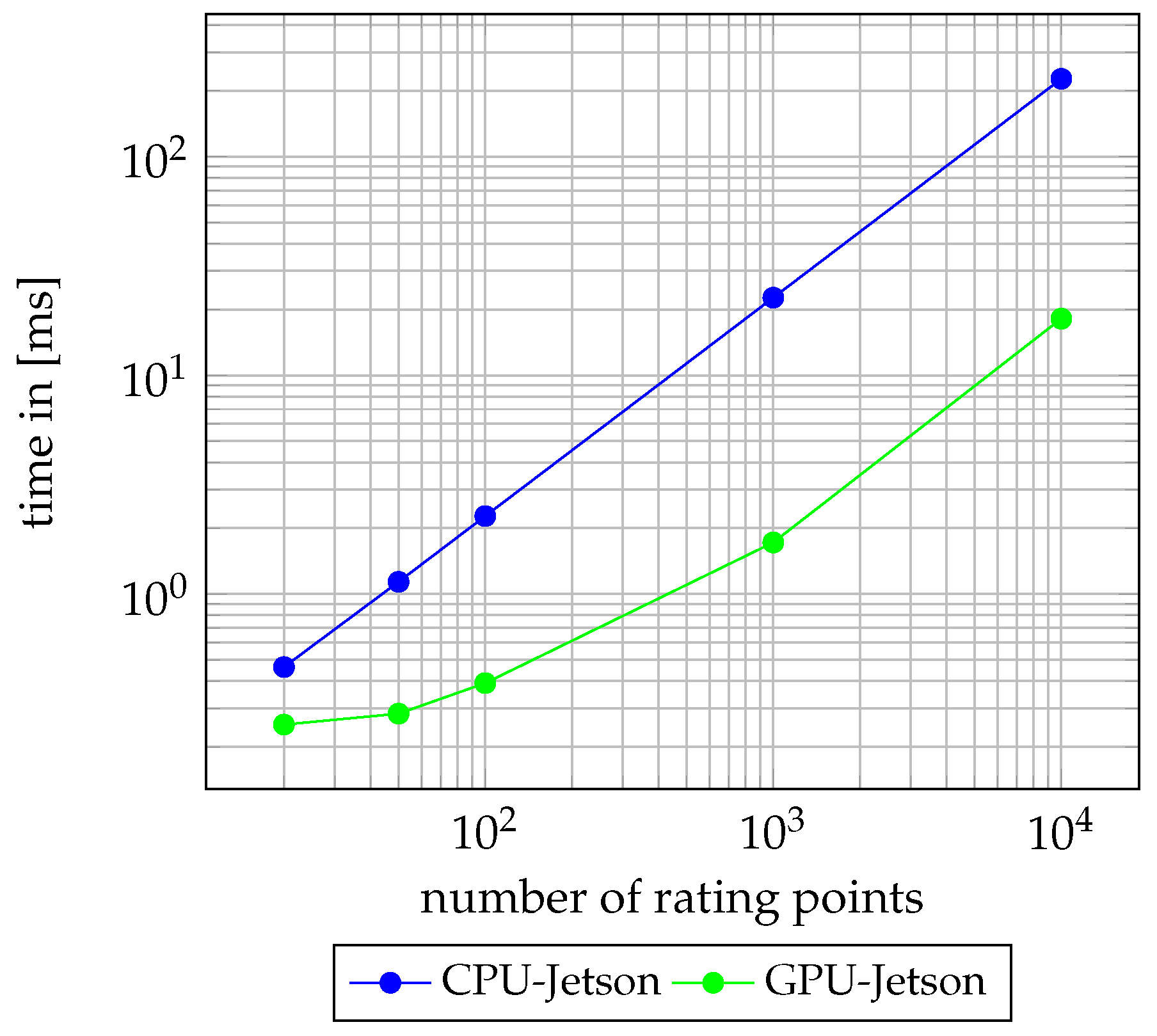
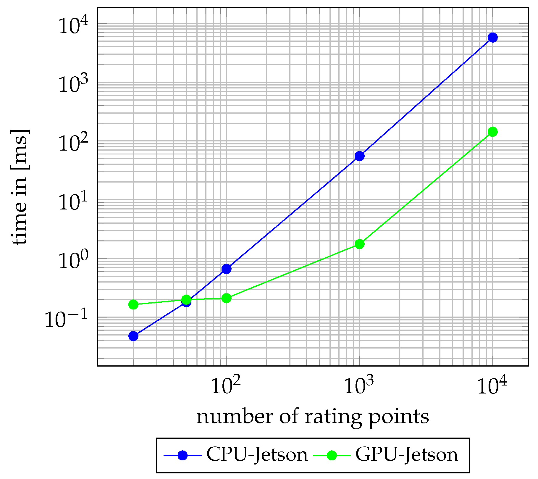
3.4. Evaluation of the Path Rating

After all paths have been planned, it is necessary to evaluate them to ensure that the vehicle drives the most convenient path. As with the other experiments, we evaluated the cost function ones with varying paths and a fixed number of rating points per path and vice versa. In Figure 9, the results of the cost functions are shown for the variation of the number of paths. The computation time on the CPU to evaluate the quality of the planned paths increases more or less linearly with the number of planned paths. However, on the GPU, the computation time is for a low number of paths nearly constant, due to the low utilization of the GPU. Only if a high number of paths is planned, the computation time is increasing with the number of planned path, because the GPU is then well utilized. For a low number of paths, the CPU is faster than the GPU. This is due to the low utilization of the GPU for a small number of paths and also the lower mathematical complexity, compared to solving the variational problem lengthwise and crosswise.
In the next experiment, the number of rating points per path was varied, and the number of paths was set again to nine. The results of this experiment are illustrated in Figure 10. The CPU is faster than the GPU for a small number of rating points per path. For higher number of rating points for each path, the GPU outperforms the CPU. The reasons for the speedup with an increased number of rating points for each path are the same as for the case of an increased number of paths, as explained in the experiment above.
Finally, it has to be answered how many paths and rating points for each path are necessary to enable a safe, comfortable, and dynamically feasible path. Generally, it can be stated that, the more paths are planned, the more likely it is to find one that meets the requirements of safety and comfort. For example, if the desired path has a narrowing, then with a higher number of planned paths it is more likely to find one with which the vehicle can pass the bottleneck in compliance with the safety criteria. A recent paper [29] from Mobileye N.V. argues that planning more than 10 4 is not reasonable for having a safe path on hand all the time. The further paths would differ only slightly, and, thus, not offer many advantages. Our experiments show that our proposed parallel algorithm is real-time capable, even if 10 4 paths are planned. To find the optimal path with 100% certainty, one would have to scan or evaluate it continuously, i.e., infinitely often. This would result in an infinite number of rating points. If a path is discretized based on the rating points, the rating points may be placed, such that it would be not recognized that a piece of the path is not within the corridor boundaries. For example, two rating points of a path are just inside the corridor boundary, but a short part of the path is outside the corridor boundaries. Since an infinite number of rating points is not possible, a number must be chosen that represents a compromise of computing time and accuracy. A rating point for every 50 cm should be sufficient for a highway scenario and all the paths for the next four seconds need to be planned ahead. Four seconds is a reasonable value since we do not have to consider any reaction time of the driver because the vehicle takes over this task. Assume that a vehicle driving on a highway at a speed of 130 km/h, which is 36 m/s. Then, the distance of the path that needs to be calculated for the future is 4 · 36 = 144 m. Correspondingly, 144 / 0.5 = 288 rating points per path should be calculated. If we look at the individual execution times of the sub-algorithms, we can see that our approach is real-time capable for 1000 paths, but not for 10,000 paths. In addition to the execution times for our path planning approach, there are also other execution times, such as for sensor data processing.

4. Conclusion and Future Work

In this work, a path planning approach based on quintic polynomials was parallelized on an embedded GPU. It was shown that the proposed path planning algorithm and its single steps can be efficiently parallelized on a GPU. Furthermore, we showed that the speedup between CPU and GPU increases with a higher number of paths and rating points per path. In addition, for a high number of paths and rating points, the GPU approach is real-time capable, which is necessary for highly automated vehicles. In the future, we want to further evaluate how many paths and rating points per path are necessary for varying real driving situations.

Author Contributions

J.F. is the main author of the paper. He implemented the algorithm, performed the evaluation and wrote the paper. S.S. and F.H. provided valuable guidance during the implementation and contributed to the writing. M.E.B. and J.T. did the technical proofing and supervised the work.

Funding

This research was funded by AUDI AG.

Conflicts of Interest

The authors declare no conflicts of interest.

Abbreviations

The following abbreviations are used in this manuscript:
ADASAdvanced Driver Assistance System
GPUGraphics Processing Unit
CPUCentral Processing Unit
ECUElectronic Control Unit
SIMTSingle Instruction Multiple Thread
SLAMSimultaneous Localization and Mapping
FMAFused Multiply Add
ROIRegion of Interest
OVMOwn Vehicle Motion
ESCSEnvironment Sensor Coordinate System
SoCSystem-on-Chip
GPGPUGeneral Purpose Computation on Graphics Processing Unit
MIMDMultiple Instruction, Multiple Data

References

  1. Taxonomy and Definitions for Terms Related to On-Road Motor Vehicle Automated Driving Systems. Available online: https://www.sae.org/standards/content/j3016_201401/ (accessed on 26 September 2018).
  2. Latombe, J.C. Robot Motion Planning; Kluwer Academic Publishers: Norwell, MA, USA, 1991. [Google Scholar]
  3. Choset, H.; Lynch, K.M.; Hutchinson, S.; Kantor, G.A.; Burgard, W.; Kavraki, L.E.; Thrun, S. Principles of Robot Motion: Theory, Algorithms, and Implementations; MIT Press: Cambridge, MA, USA, 2005. [Google Scholar]
  4. McNaughton, M.; Urmson, C.; Dolan, J.M.; Lee, J. Motion planning for autonomous driving with a conformal spatiotemporal lattice. In Proceedings of the IEEE International Conference on Robotics and Automation (ICRA), Shanghai, China, 9–13 May 2011; pp. 4889–4895. [Google Scholar] [CrossRef]
  5. Werling, M. Ein neues Konzept für die Trajektoriengenerierung und -stabilisierung in zeitkritischen Verkehrsszenarien. Ph.D. Thesis, Karlsruher Institut für Technology (KIT), Karlsruhe, Baden-Württemberg, Germany, 2011. [Google Scholar]
  6. Fassbender, D.; Müller, A.; Wuensche, H. Trajectory planning for car-like robots in unknown, unstructured environments. In Proceedings of the IEEE/RSJ International Conference on Intelligent Robots and Systems (IROS), Chicago, IL, USA, 14–18 September 2014; pp. 3630–3635. [Google Scholar] [CrossRef]
  7. Ferguson, D.; Howard, T.M.; Likhachev, M. Motion planning in urban environments. J. Field Robot. 2008, 25, 939–960. [Google Scholar] [CrossRef] [Green Version]
  8. Ziegler, J.; Stiller, C. Spatiotemporal state lattices for fast trajectory planning in dynamic on-road driving scenarios. In Proceedings of the 2009 IEEE/RSJ International Conference on Intelligent Robots and Systems, St. Louis, MO, USA, 10–15 October 2009; pp. 1879–1884. [Google Scholar] [CrossRef]
  9. Ziegler, J.; Bender, P.; Dang, T.; Stiller, C. Trajectory planning for Bertha—A local, continuous method. In Proceedings of the 2014 IEEE Intelligent Vehicles Symposium Proceedings, Dearborn, MI, USA, 8–11 June 2014; pp. 450–457. [Google Scholar] [CrossRef]
  10. Choi, J.W.; Curry, R.; Hugh Elkaim, G. Continuous Curvature Path Generation Based on Bezier Curves for Autonomous Vehicles. Int. J. Appl. Math. 2010, 40, 91–101. [Google Scholar]
  11. Ziegler, J.; Bender, P.; Schreiber, M.; Lategahn, H.; Strauss, T.; Stiller, C.; Dang, T.; Franke, U.; Appenrodt, N.; Keller, C.G.; et al. Making Bertha Drive—An Autonomous Journey on a Historic Route. IEEE Intell. Transp. Syst. Mag. 2014, 6, 8–20. [Google Scholar] [CrossRef]
  12. Gotte, C.; Keller, M.; Hass, C.; Glander, K.H.; Seewald, A.; Bertram, T. A model predictive combined planning and control approach for guidance of automated vehicles. In Proceedings of the 2015 IEEE International Conference on Vehicular Electronics and Safety (ICVES), Yokohama, Japan, 5–7 November 2015; pp. 69–74. [Google Scholar] [CrossRef]
  13. Anderson, S.J.; Karumanchi, S.B.; Iagnemma, K. Constraint-based planning and control for safe, semi-autonomous operation of vehicles. In Proceedings of the 2012 IEEE Intelligent Vehicles Symposium, Alcala de Henares, Spain, 3–7 June 2012; pp. 383–388. [Google Scholar] [CrossRef]
  14. Dafflon, B.; Gechter, F.; Gruer, P.; Koukam, A. Vehicle platoon and obstacle avoidance: A reactive agent approach. IET Intell. Transp. Syst. 2013, 7, 257–264. [Google Scholar] [CrossRef]
  15. Von Hundelshausen, F.; Himmelsbach, M.; Hecker, F.; Mueller, A.; Wuensche, H.J. Driving with Tentacles: Integral Structures for Sensing and Motion. J. Field Robot. 2008, 25, 640–673. [Google Scholar] [CrossRef]
  16. Heil, T.; Lange, A.; Cramer, S. Adaptive and efficient lane change path planning for automated vehicles. In Proceedings of the 2016 IEEE 19th International Conference on Intelligent Transportation Systems (ITSC), Rio de Janeiro, Brazil, 1–4 December 2016; pp. 479–484. [Google Scholar] [CrossRef]
  17. Burns, E.; Lemons, S.; Ruml, W.; Zhou, R. Best-first Heuristic Search for Multicore Machines. J. Artif. Intell. Res. 2010, 39, 689–743. [Google Scholar] [CrossRef]
  18. Bleiweiss, A. GPU Accelerated Pathfinding. In Proceedings of the 23rd ACM SIGGRAPH/EUROGRAPHICS Symposium on Graphics Hardware (GH), Sarajevo, Bosnia, 20–21 June 2008; pp. 65–74. [Google Scholar]
  19. Kider, J., Jr.; Henderson, M.; Likhachev, M.; Safonova, A. High-dimensional planning on the GPU. In Proceedings of the IEEE International Conference on Robotics and Automation (ICRA), Anchorage, AK, USA, 3–7 May 2010; pp. 2515–2522. [Google Scholar] [CrossRef]
  20. Cekmez, U.; Ozsiginan, M.; Sahingoz, O.K. A UAV path planning with parallel ACO algorithm on CUDA platform. In Proceedings of the International Conference on Unmanned Aircraft Systems (ICUAS), Orlando, FL, USA, 27–30 May 2014; pp. 347–354. [Google Scholar] [CrossRef]
  21. Palossi, D.; Marongiu, A.; Benini, L. On the Accuracy of Near-Optimal GPU-Based Path Planning for UAVs. In Proceedings of the 20th International Workshop on Software and Compilers for Embedded Systems (SCOPES), Sankt Goar, Germany, 12–13 June 2017; pp. 85–88. [Google Scholar] [CrossRef]
  22. Programming Guide—CUDA Toolkit Documentation. 2016. Available online: https://docs.nvidia.com/cuda/cuda-c-programming-guide/ (accessed on 25 September 2018).
  23. Grauer-Gray, S.; Killian, W.; Searles, R.; Cavazos, J. Accelerating Financial Applications on the GPU. In Proceedings of the 6th Workshop on General Purpose Processor Using Graphics Processing Units, Houston, TX, USA, 16 March 2013; pp. 127–136. [Google Scholar] [CrossRef]
  24. Bakkum, P.; Skadron, K. Accelerating SQL Database Operations on a GPU with CUDA. In Proceedings of the 3rd Workshop on General-Purpose Computation on Graphics Processing Units, Pittsburgh, PA, USA, 14 March 2010; pp. 94–103. [Google Scholar] [CrossRef]
  25. Werling, M.; Ziegler, J.; Kammel, S.; Thrun, S. Optimal trajectory generation for dynamic street scenarios in a Frenet Frame. In Proceedings of the 2010 IEEE International Conference on Robotics and Automation, Anchorage, AK, USA, 3–7 May 2010; pp. 987–993. [Google Scholar] [CrossRef]
  26. Serret, J.A. Sur quelques formules relatives à la théorie des courbes à double courbure. J. de Mathématiques Pures et Appliquées 1851, 16, 193–207. [Google Scholar]
  27. Gantmacher, F.; Brenner, J. Applications of the Theory of Matrices; Dover Publications: Mineola, NY, USA, 2005. [Google Scholar]
  28. NVIDIA Jetson TK1 Developer Kit. 2016. Available online: http://www.nvidia.com/object/jetson-tk1-embedded-dev-kit.html (accessed on 25 September 2018).
  29. Shalev-Shwartz, S.; Shammah, S.; Shashua, A. On a Formal Model of Safe and Scalable Self-driving Cars. Comput. Res. Repos. 2018, arXiv:1708.06374v5. [Google Scholar]
Figure 1. Illustration of the: (a) architecture of a desktop GPU; and (b) architecture of an embedded GPU.
Jlpea 08 00035 g001
Figure 2. The planning of one path (red arrow) is illustrated. The road consists of two lanes. The red points are the rating points of this path. These points will later be used to evaluate the course. The green dashed line is the reference path. The orange dashed lines are possibilities for endpoints of paths. The blue points are calculated endpoints of paths. The corridor boundaries are the upper lane marking and the center lane marking. For improved clarity, no paths (red arrows) are drawn to these calculated endpoints.
Jlpea 08 00035 g002
Figure 3. Transformation from ESCS to Frenet coordinates and back.
Jlpea 08 00035 g003
Figure 4. Evaluation of the cost of one path, with two rating points (red points). The road consists of only one lane. The vehicle is too far on the left part of the lane and should be guided back towards the reference path.
Jlpea 08 00035 g004
Figure 5. Evaluation of the coordinate transformation. The number of paths was varied. The number of rating points per path was always 20.
Jlpea 08 00035 g005
Figure 6. Evaluation of the coordinate transformation. The number of rating points for each path was varied. The number of paths was always nine.
Jlpea 08 00035 g006
Figure 7. In this experiment, lengthwise and crosswise path planning was evaluated. The number of rating points per path was set to 20. The number of paths was varied.
Jlpea 08 00035 g007
Figure 8. In this experiment, lengthwise and crosswise path planning was evaluated. The number of rating points per path was varied. The number of paths was set to nine.
Jlpea 08 00035 g008
Figure 9. Evaluation of the cost function. The number of paths was varied. The number of rating points per path was always 20.
Jlpea 08 00035 g009
Figure 10. Evaluation of the cost function. The number of paths was set to nine and the number of rating points for each path was varied.
Jlpea 08 00035 g010

