Article

Low-Complexity Loeffler DCT Approximations for Image and Video Coding

by
Diego F. G. Coelho
1,
Renato J. Cintra
2,3,*,
Fábio M. Bayer
4,
Sunera Kulasekera
5,
Arjuna Madanayake
6,
Paulo Martinez
3,7,
Thiago L. T. Silveira
8,
Raíza S. Oliveira
9 and
Vassil S. Dimitrov
2
1
Independent Researcher, Calgary AB, T3A 2H6, Canada
2
Department of Electrical and Computer Engineering, University of Calgary, 2500 University Dr. NW Calgary, AB T2N 1N4, Canada
3
Signal Processing Group, Departamento de Estatística, Universidade Federal de Pernambuco, Recife 50670-901, PE, Brazil
4
Departamento de Estatística and LACESM, Universidade Federal de Santa Maria, Santa Maria 97105-900, RS, Brazil
5
Department of Electrical and Computer Engineering, University of Akron, Akron, OH 44325, USA
6
Department of Electrical and Computer Engineering, Florida International University, Miami, FL 33174, USA
7
Friedrich-Alexander-Universität Erlangen-Nürnberg, 91054 Erlangen, Germany
8
Programa de Pós-Graduação em Computação, Universidade Federal do Rio Grande do Sul (UFRGS), Porto Alegre 91501-970, RS, Brazil
9
Programa de Pós-Graduação em Engenharia Elétrica, Universidade Federal de Pernambuco, Recife 50670-901, PE, Brazil
*
Author to whom correspondence should be addressed.
J. Low Power Electron. Appl. 2018, 8(4), 46; https://0-doi-org.brum.beds.ac.uk/10.3390/jlpea8040046
Submission received: 9 October 2018 / Revised: 12 November 2018 / Accepted: 16 November 2018 / Published: 22 November 2018

Abstract

:
This paper introduced a matrix parametrization method based on the Loeffler discrete cosine transform (DCT) algorithm. As a result, a new class of 8-point DCT approximations was proposed, capable of unifying the mathematical formalism of several 8-point DCT approximations archived in the literature. Pareto-efficient DCT approximations are obtained through multicriteria optimization, where computational complexity, proximity, and coding performance are considered. Efficient approximations and their scaled 16- and 32-point versions are embedded into image and video encoders, including a JPEG-like codec and H.264/AVC and H.265/HEVC standards. Results are compared to the unmodified standard codecs. Efficient approximations are mapped and implemented on a Xilinx VLX240T FPGA and evaluated for area, speed, and power consumption.

1. Introduction

Discrete time transforms have a major role in signal-processing theory and application. In particular, tools such as the discrete Haar, Hadamard, and discrete Fourier transforms, and several discrete trigonometrical transforms [1,2] have contributed to various image-processing techniques [3,4,5,6]. Among such transformations, the discrete cosine transform (DCT) of type II is widely regarded as a pivotal tool for image compression, coding, and analysis [2,7,8]. This is because the DCT closely approximates the Karhunen–Loève transform (KLT) which can optimally decorrelate highly correlated stationary Markov-I signals [2].
Indeed, the recent literature reveals a significant number of works linked to DCT computation. Some noteworthy topics are: (i) cosine–sine decomposition to compute the 8-point DCT [9]; (ii) low-complexity-pruned 8-point DCT approximations for image encoding [10]; (iii) improved 8-point approximate DCT for image and video compression requiring only 14 additions [11]; (iv) HEVC multisize DCT hardware with constant throughput, supporting heterogeneous coding unities [12]; (v) approximation of feature pyramids in the DCT domain and its application to pedestrian detection [13]; (vi) performance analysis of DCT and discrete wavelet transform (DWT) audio watermarking based on singular value decomposition [14]; (vii) adaptive approximated DCT architectures for HEVC [15]; (viii) improved Canny edge detection algorithm based on DCT [16]; and (ix) DCT-inspired feature transform for image retrieval and reconstruction [17]. In fact, several current image- and video-coding schemes are based on the DCT [18], such as JPEG [19], MPEG-1 [20], H.264 [21], and HEVC [22]. In particular, the H.264 and HEVC codecs employ low-complexity discrete transforms based on the 8-point DCT. The 8-point DCT has also been applied to dedicated image-compression systems implemented in large web servers with promising results [23]. As a consequence, several algorithms for the 8-point DCT have been proposed, such as: Lee DCT factorization [24], Arai DCT scheme [25], Feig–Winograd algorithm [26], and the Loeffler DCT algorithm [27]. Among these methods, the Loeffler DCT algorithm [27] has the distinction of achieving the theoretical lower bound for DCT multiplicative complexity [28,29].
Because the computational complexity lower bounds of the DCT have been achieved [28], the research community resorted to approximation techniques to further reduce the cost of DCT calculation. Although not capable of providing exact computation, approximate transforms can furnish very close computational results at significantly smaller computational cost. Early approximations for the DCT were introduced by Haweel [30]. Since then, several DCT approximations have been proposed. In Reference [31], Lengwehasatit and Ortega introduced a scalable approximate DCT that can be regarded as a benchmark approximation [5,31,32,33,34,35,36,37,38,39,40]. Aiming at image coding for data compression, a series of approximations have been proposed by Bouguezel-Ahmad-Swamy (BAS) [5,34,35,36,37,41]. Such approximations offer very low complexity and good coding performance [2,39].
The methods for deriving DCT approximation include: (i) application of simple functions, such as signum, rounding-off, truncation, ceil, and floor, to approximate the elements of the exact DCT matrix [30,39]; (ii) scaling and rounding-off [2,32,39,42,43,44,45,46,47]; (iii) brute-force computation over reduced search space [38,39]; (iv) inspection [33,34,35,41]; (v) single-variable matrix parametrization of existing approximations [37]; (vi) pruning techniques [48]; and (vii) derivations based on other low-complexity matrices [5]. The above-mentioned methods are capable of supplying single or very few approximations. In fact, a systematized approach for obtaining a large number of matrix approximations and a unifying scheme is lacking.
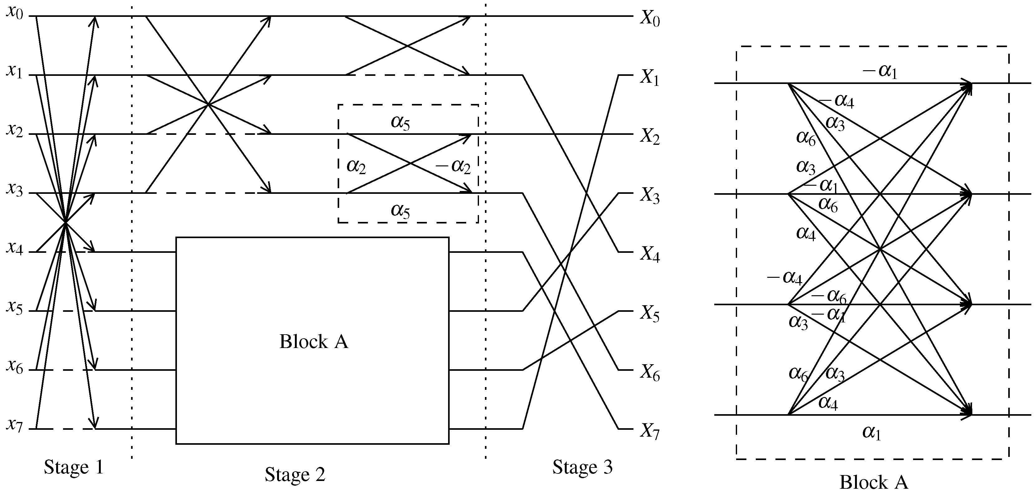
The goal of this paper is two-fold. First we aim at unifying the matrix formalism of several 8-point DCT approximations archived in the literature. For that, we consider the 8-point Loeffler algorithm as a general structure equipped with a parametrization of the multiplicands. This approach allows the definition of a matrix subspace where a large number of approximations could be derived. Second, we propose an optimization problem over the introduced matrix subspace in order to discriminate the best approximations according to several well-known figures of merit. This discrimination is important from the application point of view. It allows the user to select the transform that fits best to their application in terms of balancing performance and complexity. The optimally found approximations are subject to mathematical assessment and embedding into image- and video-encoding schemes, including the H.264/AVC and the H.265/HEVC standards. Third, we introduce hardware architecture based on optimally found approximations realized in field programmable gate array (FPGA). Although there are several subsystems in a video and image codec, this work is solely concentrated on the discrete transform subsystem.
The paper unfolds as follows. Section 2 introduces a novel DCT parametrization based on the Loeffler DCT algorithm. We provide the mathematical background and matrix properties, such as invertibility, orthogonality, and orthonormalization, are examined. Section 3 reviews the criteria employed for identifying and assessing DCT approximations, such as proximity and coding measures, and computational complexity. In Section 4, we propose a multicriteria-optimization problem aiming at deriving optimal approximation subject to Pareto efficiency. Obtained transforms are sought to be comprehensively assessed and compared with state-of-the-art competitors. 
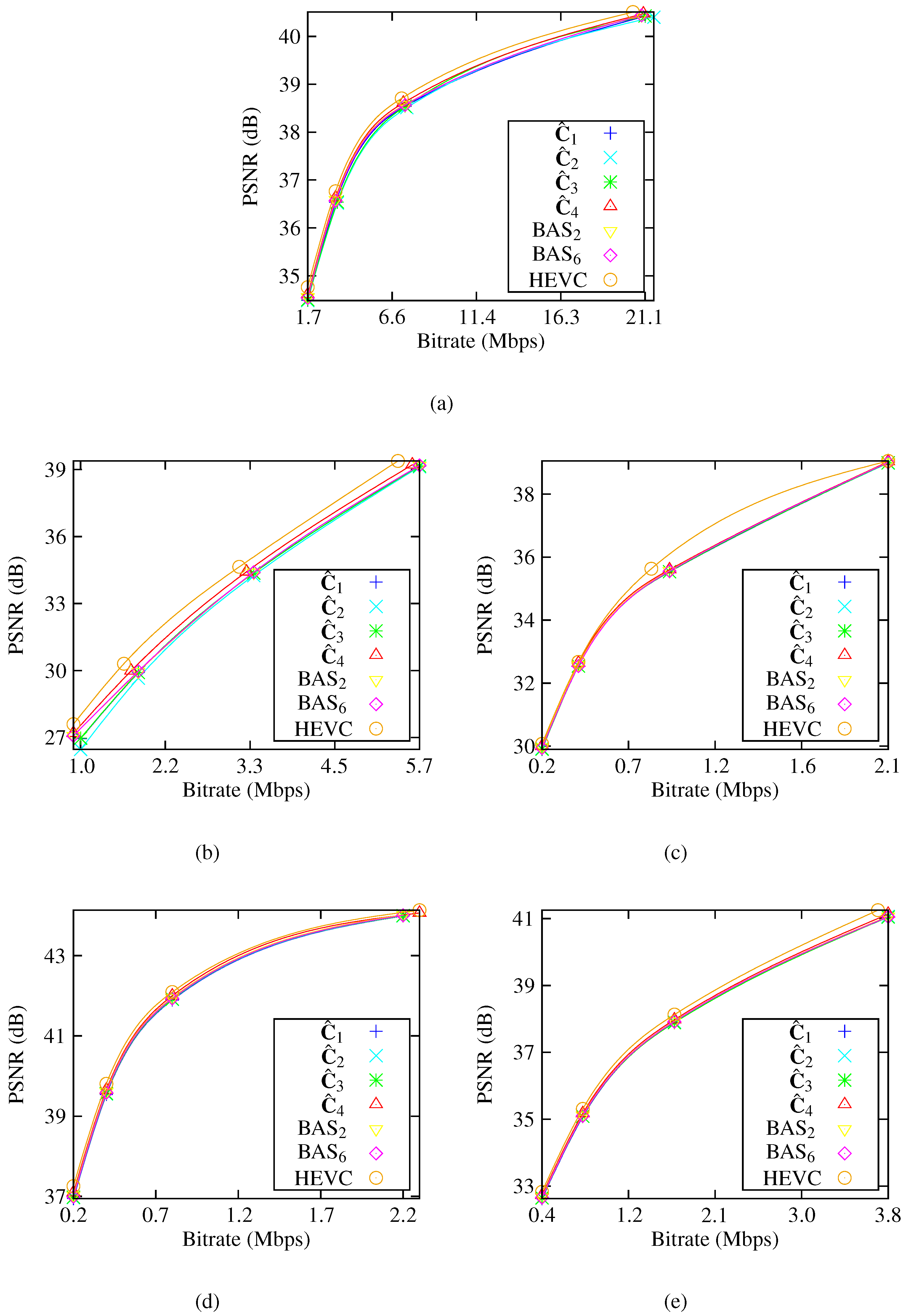
Section 5 reports the results of embedding the obtained transforms into a JPEG-like encoder, as well as in H.264/AVC and H.265/HEVC video standards. In Section 6, an FPGA hardware implementation of the optimal transformations is detailed, and the usual FPGA implementation metrics are reported. Section 7 presents our final remarks.

2. DCT Parametrization and Matrix Space

2.1. DCT Matrix Factorization

The type II DCT is defined according to the following linear transformation matrix [2,8]:
C DCT = 1 2 c 4 c 4 c 4 c 4 c 4 c 4 c 4 c 4 c 1 c 3 c 5 c 7 c 7 c 5 c 3 c 1 c 2 c 6 c 6 c 2 c 2 c 6 c 6 c 2 c 3 c 7 c 1 c 5 c 5 c 1 c 7 c 3 c 4 c 4 c 4 c 4 c 4 c 4 c 4 c 4 c 5 c 1 c 7 c 3 c 3 c 7 c 1 c 5 c 6 c 2 c 2 c 6 c 6 c 2 c 2 c 6 c 7 c 5 c 3 c 1 c 1 c 3 c 5 c 7 ,
where c k = cos ( k π / 16 ) , k = 1 , 2 , , 7 . Because several entries of C DCT are not rational, they are often truncated/rounded and represented in floating-point arithmetic [7,49], which requires demanding computational costs when compared with fixed-point schemes [5,7,33,50].
Fast algorithms can minimize the number of arithmetic operations required for the DCT computation [2,7]. A number of fast algorithms have been proposed for the 8-point DCT [24,25,26]. The vast majority of DCT algorithms consist of the following factorization [2]:
C DCT = P · M · A ,
where A is the additive matrix that represents a set of butterfly operations, M is a multiplicative matrix, and P is a permutation matrix that simply rearranges the output components to natural order. Matrix A is often fixed [2] and given by:
A = 1 0 0 0 0 0 0 1 0 1 0 0 0 0 1 0 0 0 1 0 0 1 0 0 0 0 0 1 1 0 0 0 0 0 0 1 1 0 0 0 0 0 1 0 0 1 0 0 0 1 0 0 0 0 1 0 1 0 0 0 0 0 0 1 .
Multiplicative matrix M can be further factorized. Since matrix factorization is not unique, each fast algorithm is linked to a particular factorization of M . Finally, the permutation matrix is given below:
P = 1 0 0 0 0 0 0 0 0 0 0 0 0 0 0 1 0 0 1 0 0 0 0 0 0 0 0 0 0 1 0 0 0 1 0 0 0 0 0 0 0 0 0 0 0 0 1 0 0 0 0 1 0 0 0 0 0 0 0 0 1 0 0 0 .
Among the DCT fast algorithms, the Loeffler DCT achieves the theoretical lower bound of the multiplicative complexity for 8-point DCT, which consists of 11 multiplications [27]. In this work, multiplications by irrational quantities are sought to be substituted with trivial multipliers, representable by simple bit-shifting operations (Section 2.2 and Section 3.2). Thus, we expect that approximations based on Loeffler DCT could generate low-complexity approximations. Therefore, the Loeffler DCT algorithm was separated as the starting point to devise new DCT approximations.
The Loeffler DCT employs a scaled DCT with the following transformation matrix:
C Loeffler - DCT = 2 2 · C DCT .
Such scaling eliminates one multiplicand because 2 2 · c 4 = 1 . Therefore, we can write the following expression:
C Loeffler - DCT = P · M · A ,
where
M = 2 2 · M = 1 1 1 1 0 0 0 0 1 1 1 1 0 0 0 0 2 c 2 2 c 6 2 c 6 2 c 2 0 0 0 0 2 c 6 2 c 2 2 c 2 2 c 6 0 0 0 0 0 0 0 0 2 c 1 2 c 3 2 c 5 2 c 7 0 0 0 0 2 c 5 2 c 1 2 c 7 2 c 3 0 0 0 0 2 c 3 2 c 7 2 c 1 2 c 5 0 0 0 0 2 c 7 2 c 5 2 c 3 2 c 1 .
Matrix M carries all multiplications by irrational quantities required by Loeffler fast algorithm. It can be further decomposed as:
M = B · C · D ,
where
B = 1 0 0 1 0 0 0 0 0 1 1 0 0 0 0 0 0 1 1 0 0 0 0 0 1 0 0 1 0 0 0 0 0 0 0 0 c 3 0 0 c 5 0 0 0 0 0 c 1 c 7 0 0 0 0 0 0 c 7 c 1 0 0 0 0 0 c 5 0 0 c 3 ,
C = 1 1 0 0 0 0 0 0 1 1 0 0 0 0 0 0 0 0 2 c 6 2 c 2 0 0 0 0 0 0 2 c 2 2 c 6 0 0 0 0 0 0 0 0 1 0 1 0 0 0 0 0 0 1 0 1 0 0 0 0 1 0 1 0 0 0 0 0 0 1 0 1 ,
and
D = 1 0 0 0 0 0 0 0 0 1 0 0 0 0 0 0 0 0 1 0 0 0 0 0 0 0 0 1 0 0 0 0 0 0 0 0 1 0 0 1 0 0 0 0 0 2 0 0 0 0 0 0 1 0 2 0 0 0 0 0 1 0 0 1 .
In order to achieve the minimum multiplicative complexity, the Loeffler fast algorithm uses fast rotation for the rotation blocks in matrix B and C [2,50]. Since each of the three fast rotations requires three multiplications, and we have the two additional multiplications on matrix D , the Loeffler fast algorithm requires a total of 11 multiplications.

2.2. Loeffler DCT Parametrization

DCT factorization suggests matrix parametrization. In fact, replacing multiplicands 2 · c i , i { 1 , 2 , 3 , 5 , 6 , 7 } in Matrix (8) by parameters α k , k = 1 , 2 , , 6 , respectively, yields the following parametric matrix:
M α = 1 1 1 1 0 0 0 0 1 1 1 1 0 0 0 0 α 2 α 5 α 5 α 2 0 0 0 0 α 5 α 2 α 2 α 5 0 0 0 0 0 0 0 0 α 1 α 3 α 4 α 6 0 0 0 0 α 4 α 1 α 6 α 3 0 0 0 0 α 3 α 6 α 1 α 4 0 0 0 0 α 6 α 4 α 3 α 1 ,
where subscript α = α 1 α 2 α 6 denotes a real-valued parameter vector. Mathematically, the following mapping is introduced:
f : R 6 M ( 8 ) α T α = P · M α · A ,
where M ( 8 ) represents the space of 8 × 8 matrices over the real numbers [51]. Mapping f ( · ) results in image set C ( 8 ) M ( 8 ) [51] that contains 8 × 8 matrices with the DCT matrix symmetry. In particular, for α 0 = 2 · c 1 c 2 c 3 c 5 c 6 c 7 , we have that f ( α 0 ) = C Loeffler - DCT . Other examples are α 1 = 1 1 1 1 1 1 1 and α 2 = 1 / 2 · 1 2 1 1 1 1 2 , which result in the following matrices:
T α 1 = 1 1 1 1 1 1 1 1 1 1 1 1 1 1 1 1 1 1 1 1 1 1 1 1 1 1 1 1 1 1 1 1 1 1 1 1 1 1 1 1 1 1 1 1 1 1 1 1 1 1 1 1 1 1 1 1 1 1 1 1 1 1 1 1 and T α 2 = 1 2 2 2 2 2 2 2 2 2 1 1 1 2 2 1 1 1 2 1 1 2 2 1 1 2 1 2 1 1 1 1 2 1 2 2 2 2 2 2 2 2 1 1 2 1 1 2 1 1 1 2 2 1 1 2 2 1 2 1 1 1 1 1 1 2 ,
respectively. Although the above matrices have low complexity, they may not necessarily lead to a good transform matrix in terms of mathematical properties and coding capability.
Hereafter, we adopt the following notation:
M α = E α 0 4 0 4 O α ,
where 0 4 is the the 4 × 4 null matrix, and
E α = 1 1 1 1 1 1 1 1 α 2 α 5 α 5 α 2 α 5 α 2 α 2 α 5 and O α = α 1 α 3 α 4 α 6 α 4 α 1 α 6 α 3 α 3 α 6 α 1 α 4 α 6 α 4 α 3 α 1 .
Submatrices E α and O α compute the even and odd index DCT components, respectively.

2.3. Matrix Inversion

The inverse of T α is directly given by:
T α 1 = A 1 · M α 1 · P 1 .
Because A 1 = 1 2 A = 1 2 A and P 1 = P are well-defined, nonsingular matrices, we need only check the invertibility of M α [52]. By means of symbolic computation, we obtain:
M α 1 = 1 4 · ( M α ) ,
where α = α 1 α 2 α 3 α 4 α 5 α 6 with coefficients equals to:
α 1 = 4 ( α 1 3 + 2 α 1 α 3 α 4 + α 1 α 6 2 + α 3 2 α 6 α 4 2 α 6 ) / det ( O α ) , α 2 = 16 α 2 / det ( E α ) , α 3 = 4 ( α 1 2 α 4 2 α 1 α 3 α 6 α 3 3 α 3 α 4 2 + α 4 α 6 2 ) / det ( O α ) , α 4 = 4 ( α 1 2 α 3 2 α 1 α 4 α 6 + α 3 2 α 4 α 3 α 6 2 + α 4 3 ) / det ( O α ) , α 5 = 16 α 5 / det ( E α ) , α 6 = 4 ( α 1 2 α 6 α 1 α 3 2 + α 1 α 4 2 + 2 α 3 α 4 α 6 α 6 3 ) / det ( O α ) ,
where det ( · ) returns the determinant.
Note that the expression in Matrix (18) implies that the inverse of the matrix M α is a matrix with the same structure, whose coefficients are a function of the parameter vector α . For the matrix inversion to be well-defined, we must have: det ( E α ) · det ( O α ) 0 . By explicitly computing det ( E α ) and det ( O α ) , we obtain the following condition for matrix inversion:
α 2 2 + α 5 2 0 , ( α 1 2 + α 6 2 ) 2 4 α 3 α 4 ( α 6 2 α 1 2 ) ( α 3 2 + α 4 2 ) 2 4 α 1 α 6 ( α 4 2 α 3 2 ) 1 .

2.4. Orthogonality

In this paper, we adopt the following definitions. A matrix T is orthonormal if T · T is an identity matrix [53]. If product T · T is a diagonal matrix, T is said to be orthogonal. For T α , we have that symbolic computation yields:
T α · T α = 8 0 0 0 0 0 0 0 0 2 s 1 0 2 d 0 2 d 0 0 0 0 2 s 0 0 0 0 0 0 0 2 d 0 2 s 1 0 0 0 2 d 0 0 0 0 8 0 0 0 0 2 d 0 0 0 2 s 1 0 2 d 0 0 0 0 0 0 2 s 0 0 0 0 0 2 d 0 2 d 0 2 s 1 ,
where s 0 = 2 ( α 2 2 + α 5 2 ) , s 1 = α 1 2 + α 3 2 + α 4 2 + α 6 2 , and d = α 1 ( α 4 α 3 ) + α 6 ( α 4 + α 3 ) . Thus, if d = 0 , then the transform T α is orthogonal.

2.5. Near Orthogonality

Some important and well-known DCT approximations are nonorthogonal [30,34]. Nevertheless, such transformations are nearly orthogonal [39,54]. Let A be a square matrix. Deviation from orthogonality can be quantified according to the deviation from diagonality [39] of A · A , which is given by the following expression:
δ ( A · A ) = 1 diag ( A · A ) F 2 A · A F 2 ,
where diag ( · ) returns a diagonal matrix with the diagonal elements of its argument and · F denotes the Frobenius norm [2]. Therefore, considering T α , we obtain:
δ ( T α · T α ) = 1 1 1 + 32 d 2 128 + 8 s 0 2 + 16 s 1 2 .
Nonorthogonal transforms have been recognized as useful tools. The signed DCT (SDCT) is a particularly relevant DCT approximation [30] and its deviation from orthogonality is 0.20 . We adopt such deviation as a reference value to discriminate nearly orthogonal matrices. Thus, for T α , we obtain the following criterion for near orthogonality:
0 < d 2 1 + s 0 2 16 + s 1 2 8 .

2.6. Orthonormalization

Discrete transform approximations are often sought to be orthonormal. Orthogonal transformations can be orthonormalized as described in References [2,33,53]. Based on polar decomposition [55], orthonormal or nearly orthonormal matrix C ^ α linked to T α is furnished by:
C ^ α = S α · T α , if d = 0 , S ˜ α · T α , if ( 24 ) holds true ,
where S α = T α · T α 1 , S ˜ α = diag T α · T α 1 , and · is the matrix square root [2].

3. Assessment Criteria

In this section, we describe the selected figures of merit for assessing the performance and complexity of a given DCT approximation. We separated the following performance metrics: (i) total error energy [32,54]; (ii) mean square error (MSE) [2,49]; (iii) unified coding gain [2,54], and (iv) transform efficiency [2]. For computational complexity assessment, we adopted arithmetic operation counts as figures of merit.

3.1. Performance Metrics

3.1.1. Total Error Energy

Total error energy quantifies the error between matrices in a Euclidean distance way. This measure is given by References [32,54]:
ϵ C ^ α = π · C Loeffler - DCT C ^ α F 2 .

3.1.2. Mean Square Error

The MSE of given matrix approximation C ^ α is furnished by:
MSE C ^ α = 1 8 · trace ( C Loeffler - DCT C ^ α ) · R xx · ( C Loeffler - DCT C ^ α ) ,
where R xx represents the autocorrelation matrix of a Markov I stationary process with correlation coefficient ρ , and trace ( · ) returns the sum of main diagonal elements of its matrix argument. The ( i , j ) -th entry of R xx is given by ρ | i j | , i , j = 0 , 1 , , 7 [1,2]. The correlation coefficient is assumed as equal to 0.95, which is representative for natural images [2].

3.1.3. Unified Transform Coding Gain

Unified transform coding gain provides a measure to quantify the compression capabilities of a given matrix [54]. It is a generalization of usual transform coding gain as in Reference [2]. Let g k and h k be the kth row of C ^ α and C α , respectively. Then, the unified transform coding gain is given by Reference [56]:
C g ( C ^ α ) = 10 · log 10 k = 1 8 1 ( A k · B k ) 1 8 ( dB ) ,
where A k = sum [ ( h k · h k ) R xx ] , sum ( · ) returns the sum of elements of its matrix argument, operator ∘ denotes the element-wise matrix product, B k = g k 2 2 , and · 2 is the usual vector norm.

3.1.4. Transform Efficiency

Another measure for assessing coding performance is transform efficiency [2]. Let matrix R XX = C ^ α · R xx · C ^ α be the covariance matrix of transformed signal X . The transform efficiency of C ^ α is given by [2]:
η C ^ α = trace | R XX | sum | R XX | .

3.2. Computational Cost

Based on Loeffler DCT factorization, a fast algorithm for T α is obtained and its signal flow graph (SFG) is shown in Figure 1. Stage 1, 2, and 3 correspond to matrices A , M α , and P , respectively. The computational cost of such an algorithm is closely linked to selected parameter values α k , k = 1 , 2 , , 6 . Because we aim at proposing multiplierless approximations, we restricted parameter values α k to set P = { 0 , ± 1 / 2 , ± 1 , ± 2 } , i.e., α P 6 . The elements in P correspond to trivial multiplications that affect null multiplicative complexity. In fact, the elements in P represent only additions and minimal bit-shifting operations.
The number of additions and bit-shifts can be evaluated by inspecting the discussed algorithm (Figure 1). Thus, we obtain the following expressions for the addition and bit-shifting counts, respectively:
A ( α ) = 8 + 2 · max 1 , 1 P { 0 } ( α 2 ) + 1 P { 0 } ( α 5 ) + 4 · max 1 , k { 1 , 3 , 4 , 6 } 1 P { 0 } ( α k ) ,
S ( α ) = 2 · [ 1 { ± 1 2 , ± 2 } ( α 2 ) + 1 { ± 1 2 , ± 2 } ( α 5 ) ] + 4 · k { 1 , 3 , 4 , 6 } 1 { ± 1 2 , ± 2 } ( α k ) ,
where 1 A ( x ) = 1 , if x A , and 0 otherwise.

4. Multicriteria Optimization and New Transforms

In this section, we introduce an optimization problem that aims at identifying optimal transformations derived from the proposed mapping (Matrix (13)). Considering the various performances and complexity metrics discussed in the previous section, we set up the following multicriteria optimization problem [57,58]:
min α P 6 ϵ ( C ^ α ) , MSE ( C ^ α ) , C g ( C ^ α ) , η ( C ^ α ) , A ( α ) , S ( α ) ,
subject to:
i
the existence of inverse transformation, according to the condition established in Matrix (20);
ii
the entries of the inverse matrix must be in P ; to ensure both forwarded and inverse low-complexity transformations;
iii
the property of orthogonality or near-orthogonality according to the criterion in Equation (24).
Quantities C g ( C ^ α ) and η ( C ^ α ) are in negative form to comply to the minimization requirement.
Being a multicriteria optimization problem, Problem (32) is based on objective function set F = { ϵ ( · ) , MSE ( · ) , C g ( · ) , η ( · ) , A ( · ) , S ( · ) } . The problem in analysis is discrete and finite since there is a countable number of values to the objective function. However, the nonlinear, discrete nature of the problem renders it unsuitable for analytical methods. Therefore, we employed exhaustive search methods to solve it. The discussed multicriteria problem requires the identification of the Pareto efficient solutions set [57], which is given by:
{ α P 6 : there is no α P 6 , such that f ( α ) f ( α ) for all f F and f 0 ( α ) < f 0 ( α ) for some f 0 F } .

4.1. Efficient Solutions

The exhaustive search [57] returned six efficient parameter vectors, which are listed in Table 1. For ease of notation, we denote the low-complexity matrices and their associated approximations linked to efficient solutions according to: T i T α i and C ^ i C ^ α i , respectively. Table 2 summarizes the performance metrics, arithmetic complexity, and orthonormality property of obtained matrices C ^ i , i = 1 , 2 , , 6 . We included the DCT for reference as well. Note that all DCT approximations except those by C ^ 3 are orthonormal.

4.2. Comparison

Several DCT approximations are encompassed by the proposed matrix formalism. Such transformations include: the SDCT [30], the approximation based on round-off function proposed in Reference [38], and all the DCT approximations introduced in Reference [39]. For instance, the SDCT [30] is another particular transformation fully described by the proposed matrix mapping. In fact, the SDCT can be obtained by taking f ( α 1 ) , where α 1 = 1 1 1 1 1 1 . Nevertheless, none of these approximations is part of the Pareto efficient solution set induced by the discussed multicriteria optimization problem [57]. Therefore, we compare the obtained efficient solutions with a variety of state-of-the-art 8-point DCT approximations that cannot be described by the proposed Loeffler-based formalism. We separated the Walsh–Hadamard transform (WHT) and the Bouguezel–Ahmad–Swamy (BAS) series of approximations labeled BAS 1 [34], BAS 2 [35], BAS 3 [41], BAS 4 [36], BAS 5 [37] (for a = 1 ), BAS 6 [37] (for a = 0 ), BAS 7 [37] (for a = 1 / 2 ), and BAS 8 [5]. Table 3 shows the performance measures for these transforms. For completeness, we also show the unified coding gain and the transform efficiency measures for the exact DCT [2].
Some approximations, such as the SDCT, were not explicitly included in our comparisons. Although they are in the set of matrices generated by Loeffler parametrization, they are not in the efficient solution set. Thus, we removed them from further analyses for not being an optimal solution.
In order to compare all the above-mentioned transformations, we aimed at identifying the Pareto frontiers [
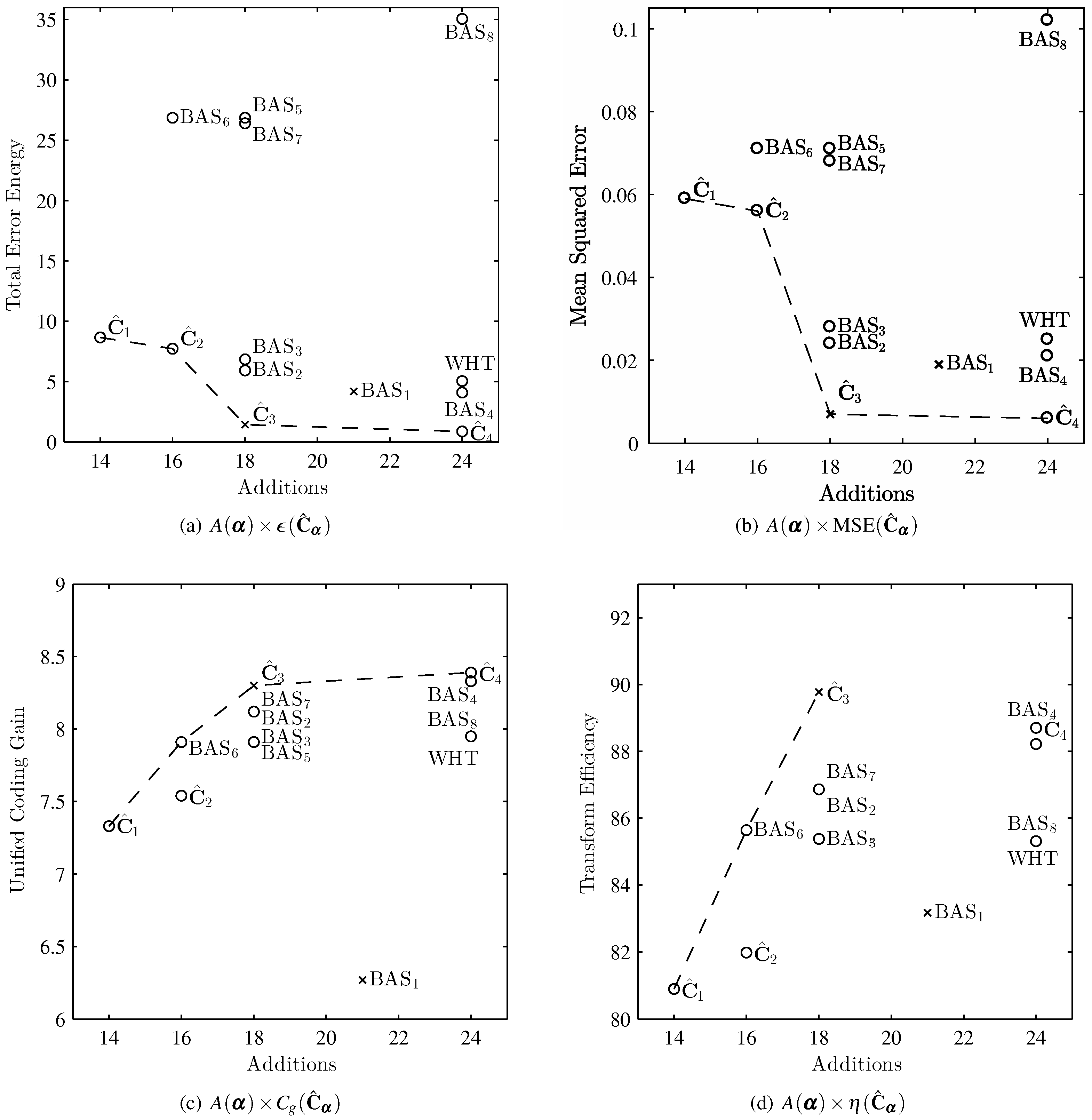
57] in two-dimensional plots considering the performance figures of the obtained efficient solution as well as the WHT and BAS approximations. Thus, we devised scatter plots considering the arithmetic complexity and performance measures. The resulting plots are shown in Figure 2. Orthogonal transform approximations are marked with circles, and nonorthogonal approximations with cross signs. The dashed curves represent the Pareto frontier [57] for each selected pair of the measures. Transformations located on the Pareto frontier are considered optimal, where the points are dominated by the frontier correspond to nonoptimal transformations. The bivariate plots in Figure 2a,b reveal that the obtained Loeffler-based DCT approximations are often situated at the optimality site prescribed by the Pareto frontier. The Loeffler approximations perform particularly well in terms of total error energy and the MSE, which capture the matrix proximity to the exact DCT matrix in a Euclidean sense. Such approximations are particularly suitable for problems that require computational proximity to the the exact transformation as in the case of detection and estimation problems [59,60]. Regarding coding performance, Figure 2c,d shows that transformations C ^ 1 , C ^ 3 , C ^ 6 , and BAS 6 are situated on the Pareto frontier, being optimal in this sense. These approximations are adequate for data compression and decorrelation [2].

5. Image and Video Experiments

5.1. Image Compression

We implemented the JPEG-like compression experiment described in References [30,34,37,41,30] and submitted the standard Elaine image to processing at a high compression rate. For quantitative assessment, we adopted the structural similarity (SSIM) index [61] and the peak signal-to-noise rate (PSNR) [8,18] measure. Figure 3 shows the reconstructed Elaine image according to the JPEG-like compression considering the following transformations: DCT, C ^ 1 , C ^ 2 , C ^ 3 , C ^ 4 , and BAS 6 . We employed fixed-rate compression and retained only five coefficients, which led to 92.1875% compression rate. Despite very low computational complexity, the approximations could furnish images with quality comparable to the results obtained from the exact DCT. In particular, approximations C ^ 1 and C ^ 2 offered good trade-off, since they required only 14–16 additions and were capable of providing competitive image quality at smaller hardware and power requirements (Section 6).
Figure 4 shows the PSNR and SSIM for different number of retained coefficients. Considering PSNR measurements, the difference between the measurements associated to the BAS 6 and to the efficient approximation were less than ≈1 dB. Similar behavior was reported when SSIM measurements were considered.

5.2. Video Compression

5.2.1. Experiments with the H.264/AVC Standard

To assess the Loeffler-based approximations in the context of video coding, we embedded them in the x264 [62] software library for encoding video streams into the H.264/AVC standard [63]. The original 8-point transform employed in H.264/AVC is a DCT-based integer approximation given by Reference [64]:
C ^ AVC = 1 8 · 8 8 8 8 8 8 8 8 12 10 6 3 3 6 10 12 8 4 4 8 8 4 4 8 10 3 12 6 6 12 3 10 8 8 8 8 8 8 8 8 6 12 3 10 10 3 12 6 4 8 8 4 4 8 8 4 3 6 10 12 12 10 6 3 .
The fast algorithm for the above transformation requires 32 additions and 14 bit-shifting operations [64].
We encoded 11 common intermediate format (CIF) videos with 300 frames from a public video database [65] using the standard and modified codec. In our simulation, we employed default settings and the resulting video quality was assessed by means of the average PSNR of chrominance and luminance representation considering all reconstructed frames. Psychovisual optimization was also disabled in order to obtain valid PSNR values and the quantization step was unaltered.
We computed the Bjøntegaard delta rate (BD-Rate) and the Bjøntegaard delta PSNR (BD-PSNR) [66] for modified codec compared to the usual H.264 native DCT approximation. BD-Rate and BD-PSNR were automatically furnished by the x264 [62] software library. A comprehensive review of Bjøntegaard metrics and their specific mathematical formulations can be found in Reference [67]. For that, we followed the procedure specified in References [66,67,68]. We adopted the same testing point as determined in Reference [69] with fixed quantization parameter (QP) in { 22 , 27 , 32 , 37 } . Following References [67,68], we employed cubic spline interpolation between the testing points for better visualization.
Figure 5 shows the resulting average BD-Rate distortion curves for the selected videos, where H.264 represents the integer DCT used in the x264 software library shown in Matrix (34). We note the superior performance of C ^ 3 and C ^ 4 approximations compared to BAS 2 and BAS 6 transforms. This performance is more evident for small bitrates. As the bitrate increases, the quality performance of C ^ 3 , C ^ 4 , BAS 2 , and BAS 6 approximates native DCT implementation. Table 4 shows the BD-Rate and BD-PSNR measures for the 11 CIF video sequence selected from Reference [65].
Figure 6a–f displays the first encoded frame of the ‘Foreman’ video sequence at QP = 27 according to the modified coded based on the proposed efficient approximations and BAS approximations. For reference, Figure 6g shows the resulting frame obtained from the standard H.264.
Note that Loeffler approximations C ^ 1 and C ^ 2 , again, show better performance in terms of BD-PSNR measures than BAS transforms BAS 2 and BAS 6 . We attribute the difference in quality between C ^ 3 and C ^ 4 in relation to C ^ 1 and C ^ 2 to the associated complexity discrepancy as depicted in Table 2. The reduction in the number of additions and bit-shifting operations come at the expense of performance.

5.2.2. Experiments with the H.265/HEVC Standard

We also embedded Loeffler-based approximations into the HM-16.3 H.265/HEVC reference software [70]. The H.265/HEVC employs the following integer transform:
C ^ HEVC = 1 64 · 64 64 64 64 64 64 64 64 89 75 50 18 18 50 75 89 83 36 36 83 83 36 36 83 75 18 89 50 50 89 18 75 64 64 64 64 64 64 64 64 50 89 18 75 75 18 89 50 36 83 83 36 36 83 83 36 18 50 75 89 89 75 50 18 ,
which demands 72 additions and 62 bit-shifting operations, when considering the factorization method based on odd and even decomposition described in Reference [2]. Besides a particular 8-point integer transformation, the HEVC standard also employs 4-, 16-, and 32-point transforms [22]. To obtain a modified version of the H.265/HEVC codec, we derived 16- and 32-point approximations based on the scalable recursive method proposed in Reference [71]. The 8-point Loeffler-based efficient solutions were employed as fundamental building blocks for scaling up. Since the 4-point DCT matrix only possesses integer coefficients, it was employed unaltered. The additive complexity of the scaled 16- and 32-point approximations is 2 · A ( α ) + 16 and 4 · A ( α ) + 64 , respectively [71]. For the bit-shifting count, we have 2 · S ( α ) and 4 · S ( α ) , respectively.
In order to perform image-quality assessment, we encoded the first 100 frames of one standard sequence of each A to F video classes defined in the Common Test Conditions and Software Reference Configurations (CTCSRC) document [72]. The selected videos and their attributes are made explicit in the first two columns of Table 5. Classes A and B present high-resolution content for broadcasting and video on demand services; Classes C and D are lower-resolution contents for the same applications; Class E reflects typical examples of video-conferencing data; and Class F provides computer-generated image sequences [73]. All encoding parameters, including QP values, were set according to the CTCSRC document for the Main profile and All-Intra (AI), Random Access (RA), Low Delay B (LD-B), and Low Delay P (LD-P) configurations. In the AI configuration, each frame from the input video sequence is independently coded. RA and LD (B and P) coding modes differ mainly by order of coding and outputting. In the former, the coding order and output order of the pictures (frames) may differ, whereas equal order is required for the latter (Reference [74], p. 94). RA configuration relates to broadcasting and streaming use, whereas LD (B and P) represent conventional applications.
It is worth mentioning that Class A test sequences are not used for LDB and LDP coding tests, whereas Class E videos are not included in the RA test cases because of the nature of the content they represent (Reference [74], p. 93).
As figures of merit, we computed the BD-Rate and BD-PSNR for the modified versions of the codec. Figure 7, Figure 8, Figure 9 and Figure 10 depict the rate-distortion curves and Table 5 presents the Bjøntegaard metrics for the considered sets of 8- to 32-point approximations for modes AI, RA, LDB, and LDP. BD-Rate and BD-PSNR are also automatically furnished by HM-16.3 H.265/HEVC reference software [70]. We employed the cubic spline interpolation based on four testing points on Figure 7, Figure 8, Figure 9 and Figure 10, as specified in References [67,68]. The curves denoted by HEVC represents the native integer approximations for the 8-, 16-, and 32-point DCT in the HM-16.3 H.265/HEVC software [70]. These four testing points were determined by the specification for HEVC as in Reference [69] with fixed QP { 22 , 27 , 32 , 37 } . One can note that there is no significant image-quality degradation when considering approximate transforms. Furthermore, in all the cases, it can be seen that C ^ 4 performs better with a degradation of no more than 0.52 dB.
The Loeffler-based approximations could present competitive image quality while possessing low computational complexity. Table 6 shows the arithmetic costs of both the original and modified extended versions, and the H.265/HEVC native transform. As a qualitative result, Figure 11 depicts the first frame of the ‘BasketballDrive’ video sequence resulting from the unmodified H.265/HEVC [70] and from the modified codec according to the discussed approximations and their scaled versions at QP = 32 . We also display the related frames according to the BAS 2 and BAS 6 transforms.

6. FPGA Implementation

To compare the hardware-resource consumption of the discussed approximations, they were initially modeled and tested in Matlab Simulink and then physically realized on FPGA. The FPGA used was a Xilinx Virtex-6 XC6VLX240T installed on a Xilinx ML605 prototyping board. FPGA realization was tested with 100,000 random 8-point input test vectors using hardware cosimulation. Test vectors were generated from within the Matlab environment and routed to the physical FPGA device using a JTAG-based hardware cosimulation. Then, measured data from the FPGA was routed back to Matlab memory space.
We separated the BAS 6 approximation for comparison with efficient approximations because its performance metrics lay on the Pareto frontier of the plots in Figure 2. The associated FPGA implementations were evaluated for hardware complexity and real-time performance using metrics such as configurable logic blocks (CLB) and flip-flop (FF) count, critical path delay ( T cpd ) in ns, and maximum operating frequency ( F max ) in MHz. Values were obtained from the Xilinx FPGA synthesis and place-route tools by accessing the xflow.results report file. In addition, static ( Q p ) and dynamic power ( D p in mW / GHz ) consumption were estimated using the Xilinx XPower Analyzer. We also reported area-time complexity ( A T ) and area-time-squared complexity ( A T 2 ). Circuit area (A) was estimated using the CLB count as a metric, and time was derived from T cpd . Table 7 lists the FPGA hardware resource and power consumption for each algorithm.
Considering the circuit complexity of the discussed approximations and BAS 6 [5], as measured from the CBL count for the FPGA synthesis report, it can be seen from Table 7 that T 1 is the smallest option in terms of circuit area. When considering maximum speed, matrix T 5 showed the best performance on the Vertex-6 XC6VLX240T device. Alternatively, if we consider the normalized dynamic power consumption, the best performance was again measured from T 1 .

7. Conclusions and Final Remarks

In this paper, we introduced a mathematical framework for the design of 8-point DCT approximations. The Loeffler algorithm was parameterized and a class of matrices was derived. Matrices with good properties, such as low-complexity, invertibility, orthogonality or near-orthogonality, and closeness to the exact DCT, were separated according to a multicriteria optimization problem aiming at Pareto efficiency. The DCT approximations in this class were assessed, and the optimal transformations were separated.
The obtained transforms were assessed in terms of computational complexity, proximity, and coding measures. The derived efficient solutions constitute DCT approximations capable of good properties when compared to existing DCT approximations. At the same time, approximation requires extremely low computation costs: only additions and bit-shifting operations are required for their evaluation.
We demonstrated that the proposed method is a unifying structure for several approximations scattered in the literature, including the well-known approximation by Lengwehasatit–Ortega [31], and they share the same matrix factorization scheme. Additionally, because all discussed approximations have a common matrix expansion, the SFG of their associated fast algorithms are identical except for the parameter values. Thus, the resulting structure paves the way to performance-selectable transforms according to the choice of parameters.
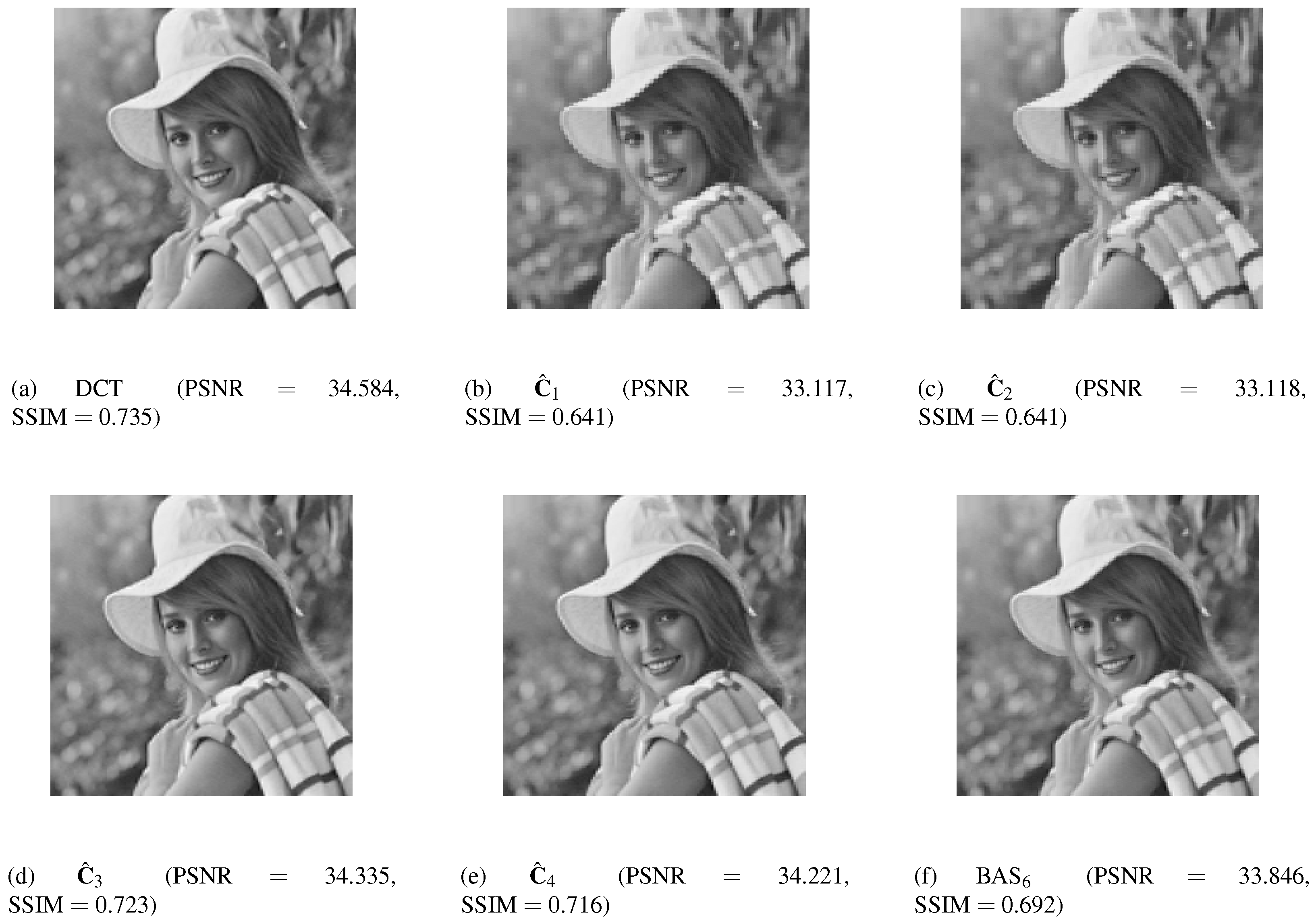
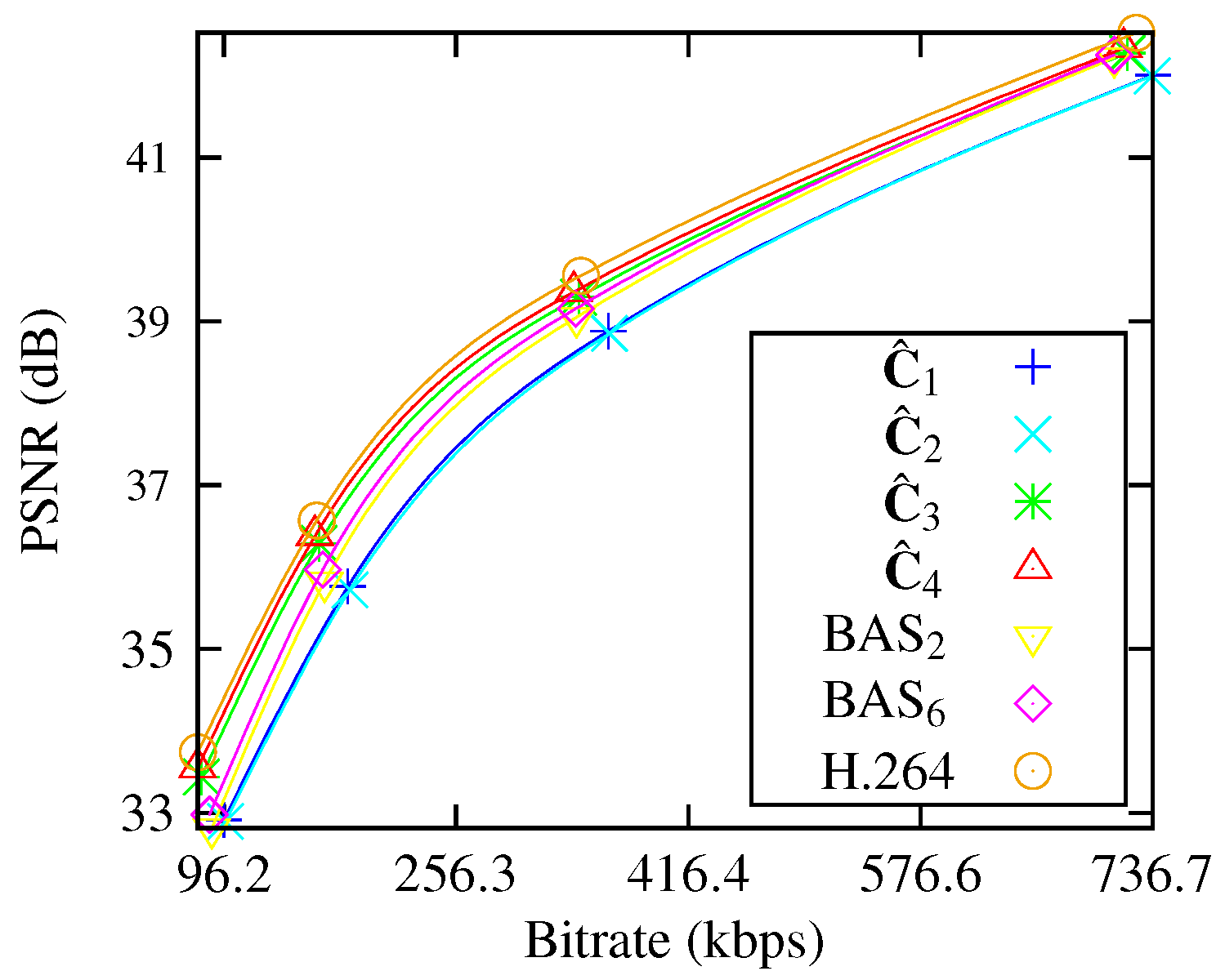
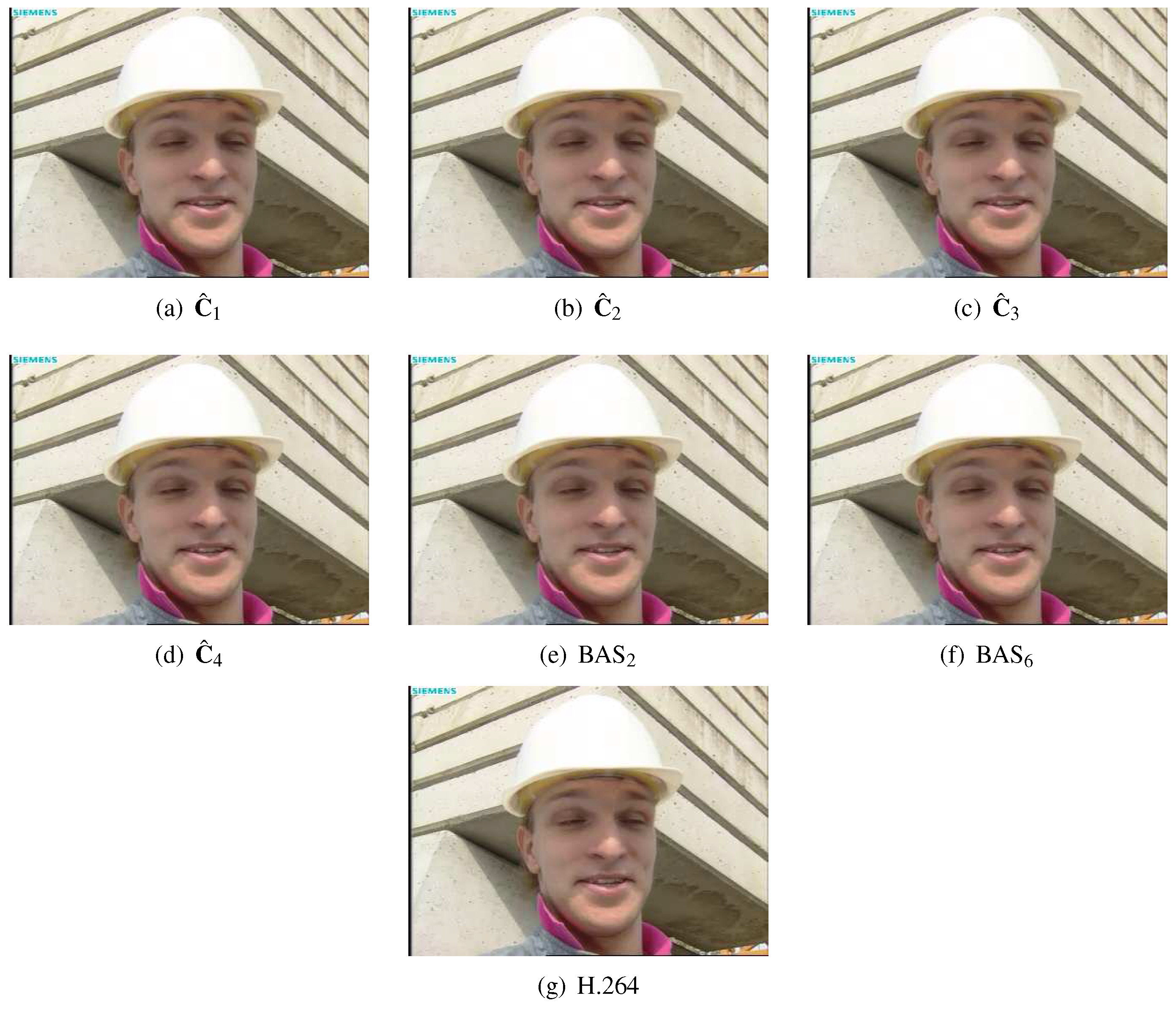
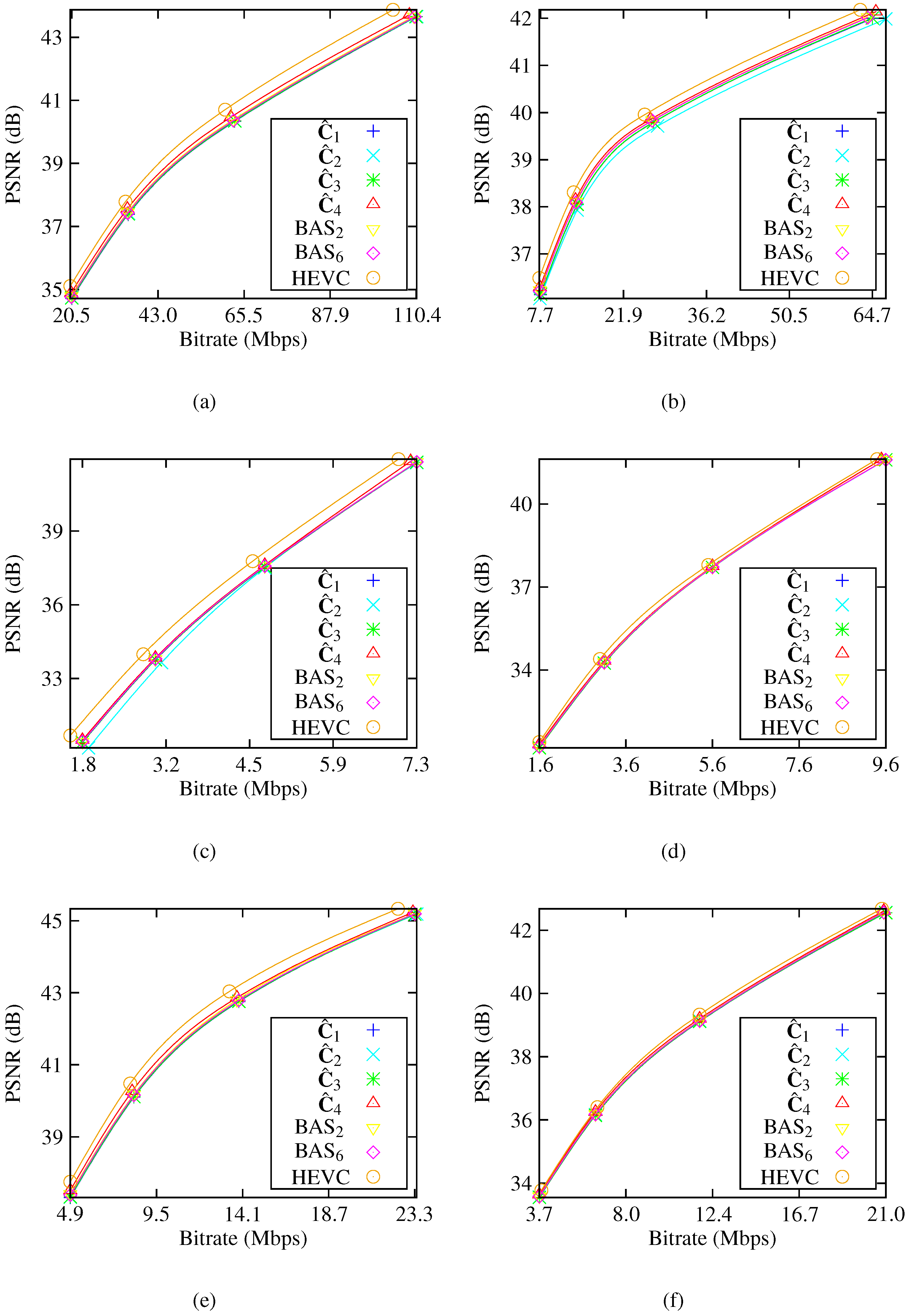
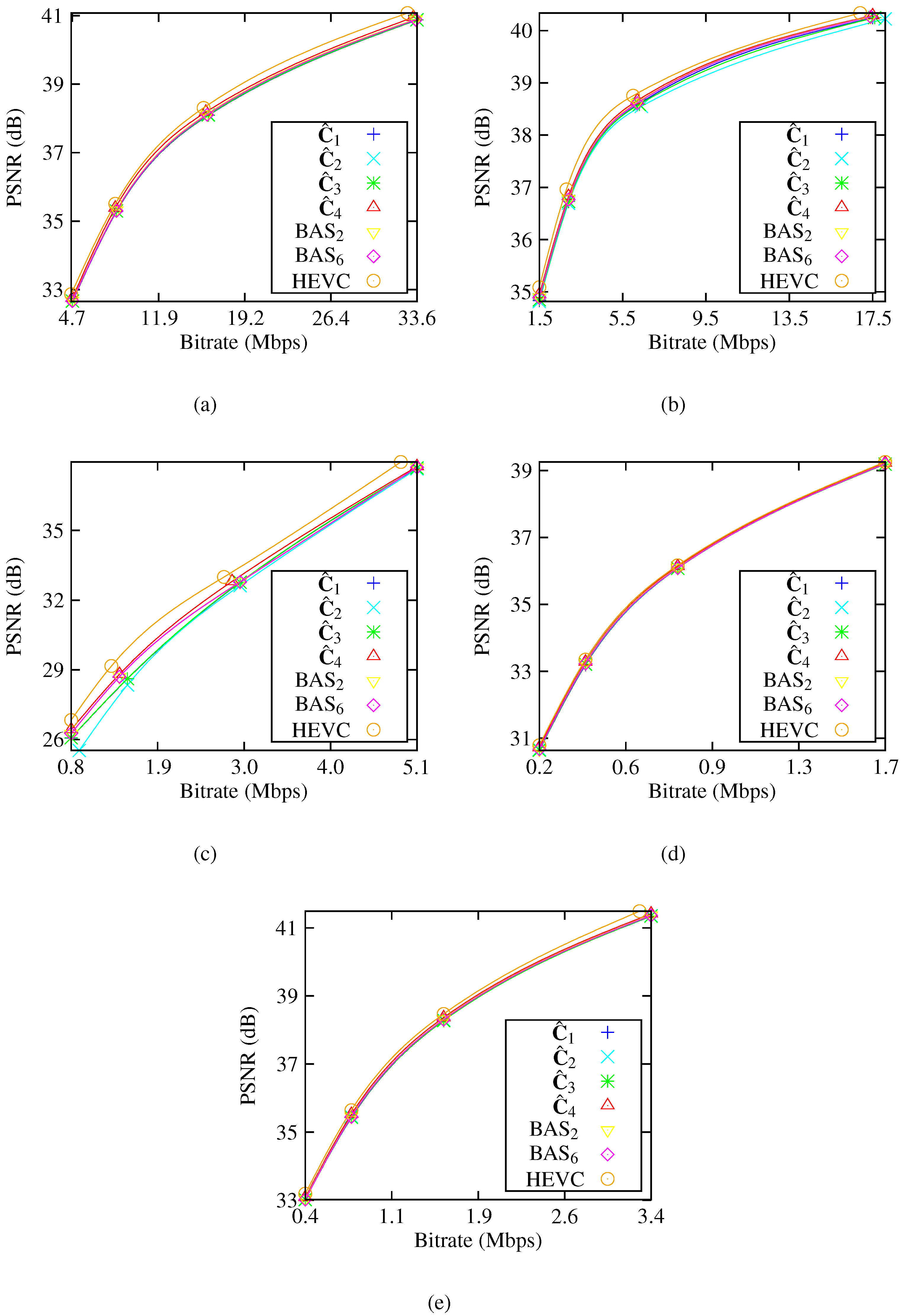
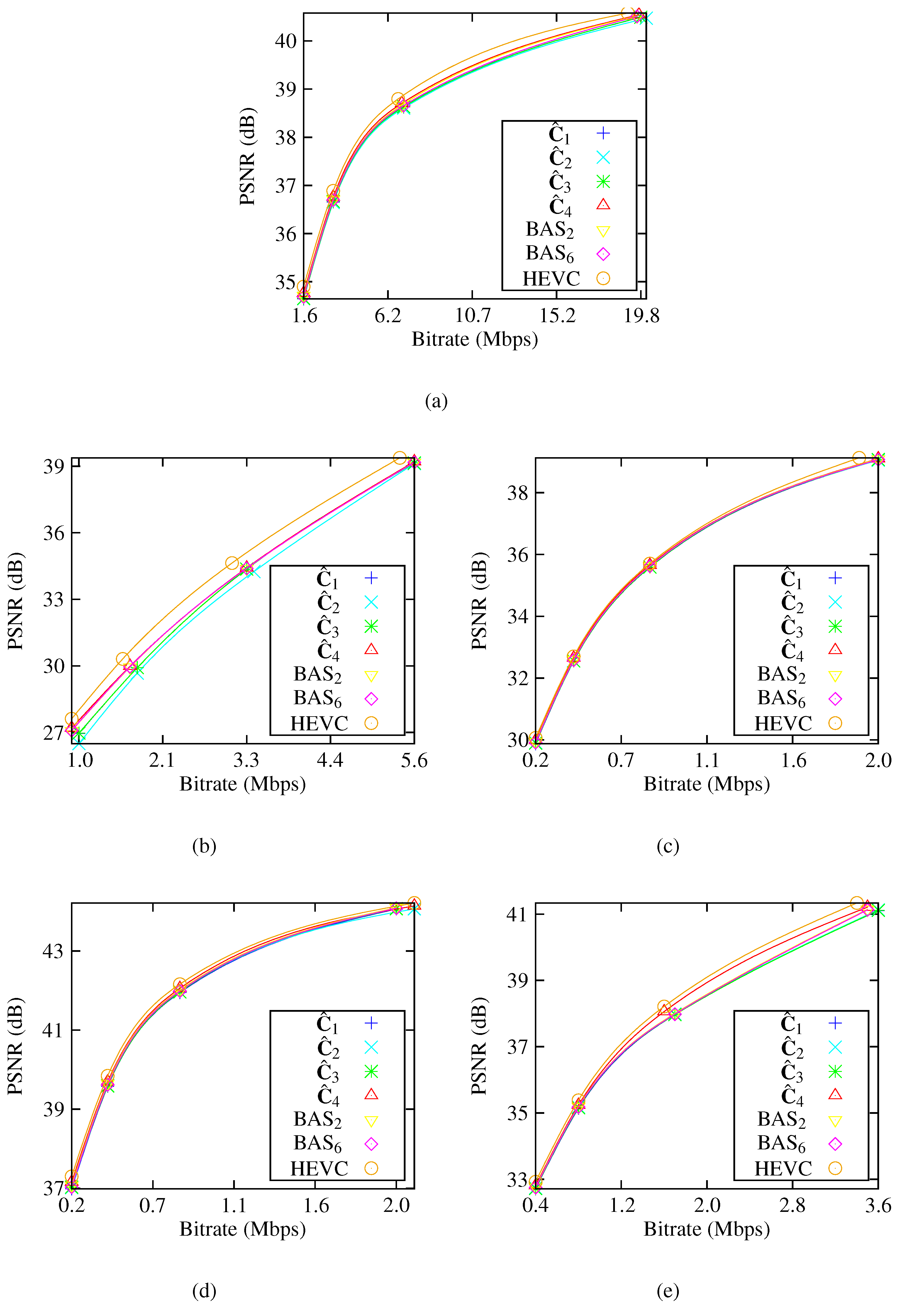
Moreover, approximations were assessed and compared in terms of image and video coding. For images, a JPEG-like encoding simulation was considered, and for videos, approximations were embedded in the H.264/AVC and H.265/HEVC video-coding standards. Approximations exhibited good coding performance compared to exact DCT-based JPEG compression and the obtained frame video quality was very close to the results shown by the H.264/AVC and H.265/HEVC standards.
Extensions for larger blocklengths can be achieved by considering scalable approaches such as the one suggested in Reference [71]. Alternatively, one could employ direct parameterization of the 16-point Loeffler DCT algorithm described in Reference [27].

Author Contributions

Conceptualization, D.F.G.C. and R.J.C.; methodology, D.F.G.C. and R.J.C.; software, T.L.T.S., P.M. and R.S.O.; hardware, S.K., R.S.O., and A.M.; validation, D.F.G.C., R.J.C., T.L.T.S., P.M. and R.S.O.; writing—original draft preparation, D.F.G.C. and R.J.C.; writing, reviewing, and editing, D.F.G.C., R.J.C., T.L.T.S., R.S.O., F.M.B. and S.K.; supervision, R.J.C.; funding acquisition, R.J.C. and V.S.D.

Funding

Partial support from CAPES, CNPq, FACEPE, and FAPERGS.

Conflicts of Interest

The authors declare no conflict of interest.

Abbreviations

The following abbreviations are used in this manuscript:
DCTDiscrete cosine transform
AVCAdvanced video coding
HEVCHigh-efficiency video coding
FPGAField-programmable gate array
KLTKarhunen–Loève transform
DWTDiscrete wavelet transform
JPEGJoint photographic experts group
MPEGMoving-picture experts group
MSEMean-squared error
SSIMStructural similarity index metric
PSNRPeak signal-to-noise ratio
WHTWalsh–Hadamard transform
QPQuantization parameter
BDBjøntegaard delta
CIFCommon intermediate format
CLBConfigurable logic block
FFFlip-flop

References

  1. Ahmed, N.; Rao, K.R. Orthogonal Transforms for Digital Signal Processing; Springer: New York, NY, USA, 1975. [Google Scholar]
  2. Britanak, V.; Yip, P.; Rao, K.R. Discrete Cossine and Sine Transforms; Academic Press: Orlando, FL, USA, 2007. [Google Scholar]
  3. Kolaczyk, E.D. Methods for analyzing certain signals and images in astronomy using Haar wavelets. In Proceedings of the Asilomar Conference on Signals, Systems & Computers, Pacific Grove, CA, USA, 2–5 November 1997; Volume 1, pp. 80–84. [Google Scholar]
  4. Qiang, Y. Image denoising based on Haar wavelet transform. In Proceedings of the International Conference on Electronics and Optoelectronics, Dalian, China, 29–31 July 2011; Volume 3. [Google Scholar]
  5. Bouguezel, S.; Ahmad, M.O.; Swamy, M.N.S. Binary Discrete Cosine and Hartley Transforms. IEEE Trans. Circuits Syst. I 2013, 60, 989–1002. [Google Scholar] [CrossRef]
  6. Martucci, S.A.; Mersereau, R.M. New Approaches To Block Filtering of Images Using Symmetric Convolution and the DST or DCT. In Proceedings of the International Symposium on Circuits and Systems, Chicago, IL, USA, 3–6 May 1993; pp. 259–262. [Google Scholar]
  7. Oppenheim, A.V.; Schafer, R.W.; Buck, J.R. Discrete-Time Signal Processing, 2nd ed.; Prentice-Hall, Inc.: Upper Saddle River, NJ, USA, 1999; Volume 1. [Google Scholar]
  8. Gonzalez, R.C.; Woods, R.E. Digital Image Processing, 2nd ed.; Prentice-Hall, Inc.: Upper Saddle River, NJ, USA, 2001. [Google Scholar]
  9. Parfieniuk, M. Using the CS decomposition to compute the 8-point DCT. In Proceedings of the IEEE International Symposium on Circuits and Systems (ISCAS), Lisbon, Portugal, 24–27 May 2015; pp. 2836–2839. [Google Scholar]
  10. Coutinho, V.D.A.; Cintra, R.J.; Bayer, F.M.; Kulasekera, S.; Madanayake, A. Low-complexity pruned 8-point DCT approximations for image encoding. In Proceedings of the International Conference on Electronics, Communications and Computers (CONIELECOMP), Cholula, Mexico, 25–27 February 2015; pp. 1–7. [Google Scholar]
  11. Potluri, U.S.; Madanayake, A.; Cintra, R.J.; Bayer, F.M.; Kulasekera, S.; Edirisuriya, A. Improved 8-point Approximate DCT for Image and Video Compression Requiring Only 14 Additions. IEEE Trans. Circuits Syst. I 2014, 61, 1727–1740. [Google Scholar] [CrossRef]
  12. Goebel, J.; Paim, G.; Agostini, L.; Zatt, B.; Porto, M. An HEVC multi-size DCT hardware with constant throughput and supporting heterogeneous CUs. In Proceedings of the IEEE International Symposium on Circuits and Systems (ISCAS), Montreal, QC, Canada, 22–25 May 2016; pp. 2202–2205. [Google Scholar]
  13. Naiel, M.A.; Ahmad, M.O.; Swamy, M.N.S. Approximation of feature pyramids in the DCT domain and its application to pedestrian detection. In Proceedings of the IEEE International Symposium on Circuits and Systems (ISCAS), Montreal, QC, Canada, 22–25 May 2016; pp. 2711–2714. [Google Scholar]
  14. Lalitha, N.V.; Prasad, P.V.; Rao, S.U. Performance analysis of DCT and DWT audio watermarking based on SVD. In Proceedings of the International Conference on Circuit, Power and Computing Technologies (ICCPCT), Nagercoil, India, 18–19 March 2016; pp. 1–5. [Google Scholar]
  15. Masera, M.; Martina, M.; Masera, G. Adaptive Approximated DCT Architectures for HEVC. IEEE Trans. Circuits Syst. Video Technol. 2017, 27, 2714–2725. [Google Scholar] [CrossRef]
  16. Zhao, M.; Liu, H.; Wan, Y. An improved Canny edge detection algorithm based on DCT. In Proceedings of the IEEE International Conference on Progress in Informatics and Computing (PIC), Nanjing, China, 18–20 December 2015; pp. 234–237. [Google Scholar]
  17. Wang, Y.; Shi, M.; You, S.; Xu, C. DCT Inspired Feature Transform for Image Retrieval and Reconstruction. IEEE Trans. Image Process. 2016, 25, 4406–4420. [Google Scholar] [CrossRef] [PubMed] [Green Version]
  18. Bhaskaran, V.; Konstantinides, K. Image and Video Compression Standards; Kluwer Academic Publishers: Norwell, MA, USA, 1997. [Google Scholar]
  19. Wallace, G.K. The JPEG still picture compression standard. IEEE Trans. Consum. Electron. 1992, 38, xviii–xxxiv. [Google Scholar] [CrossRef]
  20. Roma, N.; Sousa, L. Efficient hybrid DCT-domain algorithm for video spatial downscaling. EURASIP J. Adv. Signal Process. 2007, 2007, 057291. [Google Scholar] [CrossRef]
  21. Wiegand, T.; Sullivan, G.J.; Bjøntegaard, G.; Luthra, A. Overview of the H.264/AVC video coding standard. IEEE Trans. Circuits Syst. Video Technol. 2003, 13, 560–576. [Google Scholar] [CrossRef] [Green Version]
  22. Pourazad, M.T.; Doutre, C.; Azimi, M.; Nasiopoulos, P. HEVC: The New Gold Standard for Video Compression: How Does HEVC Compare with H.264/AVC? IEEE Consum. Electron. Mag. 2012, 1, 36–46. [Google Scholar] [CrossRef]
  23. Horn, D.R. Lepton Image Compression: Saving 22% Losslessly from Images at 15MB/s. 2016. Available online: https://blogs.dropbox.com/tech/2016/07/lepton-image-compression-saving-22-losslessly-from-images-at-15mbs/ (accessed on 10 November 2018).
  24. Lee, B. A New Algorithm to Compute the Discrete Cosine Transform. IEEE Trans. Acoust. Speech Signal Process. 1984, 32, 1243–1245. [Google Scholar]
  25. Arai, Y.; Agui, T.; Nakajima, M. A fast DCT-SQ scheme for images. IEICE Trans. 1988, E71, 1095–1097. [Google Scholar]
  26. Feig, E.; Winograd, S. Fast Algorithms for the Discrete Cosine Transform. IEEE Trans. Signal Process. 1992, 40, 2174–2193. [Google Scholar] [CrossRef]
  27. Loeffler, C.; Ligtenberg, A.; Moschytz, G.S. Practical Fast 1-D DCT Algorithms with 11 Multiplications. In Proceedings of the International Conference on Acoustics, Speech, and Signal Processing, Glasgow, UK, 23–26 May 1989; Volume 2, pp. 988–991. [Google Scholar]
  28. Duhamel, P.; H’Mida, H. New 2n DCT algorithms suitable for VLSI implementation. In Proceedings of the IEEE International Conference on Acoustics, Speech, and Signal Processing, Dallas, TX, USA, 6–9 April 1987; Volume 12, pp. 1805–1808. [Google Scholar]
  29. Heideman, M.T.; Burrus, C.S. Multiplicative Complexity, Convolution, and the DFT; Springer: New York, NY, USA, 1988. [Google Scholar]
  30. Haweel, T.I. A new square wave transform based on the DCT. Signal Process. 2001, 81, 2309–2319. [Google Scholar] [CrossRef]
  31. Lengwehasatit, K.; Ortega, A. Scalable Variable Complexity Approximate Forward DCT. IEEE Trans. Circuits Syst. Syst. Video Technol. 2004, 14, 1236–1248. [Google Scholar] [CrossRef] [Green Version]
  32. Cintra, R.J.; Bayer, F.M. A DCT approximation for image compression. IEEE Signal Process. Lett. 2011, 18, 579–582. [Google Scholar] [CrossRef]
  33. Bayer, F.M.; Cintra, R.J. DCT-like transform for image compression requires 14 additions only. Electron. Lett. 2012, 48, 919–921. [Google Scholar] [CrossRef]
  34. Bouguezel, S.; Ahmad, M.O.; Swamy, M.N.S. A multiplication-free transform for image compression. In Proceedings of the 2nd International Conference on Signals, Circuits and Systems, Monastir, Tunisia, 7–9 November 2008; pp. 1–4. [Google Scholar]
  35. Bouguezel, S.; Ahmad, M.O.; Swamy, M.N.S. Low-complexity 8x8 transform for image compression. Electron. Lett. 2008, 44, 1249–1250. [Google Scholar] [CrossRef]
  36. Bouguezel, S.; Ahmad, M.O.; Swamy, M.N.S. A novel transform for image compression. In Proceedings of the 53rd IEEE International Midwest Symposium on Circuits and Systems, Seattle, WA, USA, 1–4 August 2010; pp. 509–512. [Google Scholar]
  37. Bouguezel, S.; Ahmad, M.O.; Swamy, M.N.S. A low-complexity parametric transform for image compression. In Proceedings of the IEEE International Symposium on Circuits and Systems, Rio de Janeiro, Brazil, 15–18 May 2011; pp. 2145–2148. [Google Scholar]
  38. Cintra, R.J. An Integer Approximation Method for Discrete Sinusoidal Transforms. Circuits Syst. Signal Process. 2011, 30, 1481–1501. [Google Scholar] [CrossRef]
  39. Cintra, R.J.; Bayer, F.M.; Tablada, C.J. Low-complexity 8-point DCT approximations based on integer functions. Signal Process. 2014, 99, 201–214. [Google Scholar] [CrossRef] [Green Version]
  40. Zhang, D.; Lin, S.; Zhang, Y.; Yu, L. Complexity controllable {DCT} for real-time H.264 encoder. J. Vis. Commun. Image Represent. 2007, 18, 59–67. [Google Scholar] [CrossRef]
  41. Bouguezel, S.; Ahmad, M.O.; Swamy, M.N.S. A fast 8×8 transform for image compression. In Proceedings of the International Conference on Microelectronics, Columbus, OH, USA, 4–7 August 2009; pp. 74–77. [Google Scholar]
  42. Chen, Y.J.; Oraintara, S.; Tran, T.D.; Amaratunga, K.; Nguyen, T.Q. Multiplierless approximation of transforms using lifting scheme and coordinate descent with adder constraint. In Proceedings of the IEEE International Conference on Acoustics, Speech, and Signal Processing, Orlando, FL, USA, 13–17 May 2002; Volume 3. [Google Scholar]
  43. Liang, M.J.; Tran, T.D. Approximating the DCT with the lifting scheme: Systematic design and applications. In Proceedings of the Asilomar Conference on Signals, Systems and Computers, Pacific Grove, CA, USA, 29 October–1 November 2000; Volume 1, pp. 192–196. [Google Scholar]
  44. Liang, M.J.; Tran, T.D. Fast multiplierless approximations of the DCT with the lifting scheme. IEEE Trans. Signal Process. 2001, 49, 3032–3044. [Google Scholar] [CrossRef] [Green Version]
  45. Malvar, H. Fast computation of discrete cosine transform through fast Hartley transform. Electron. Lett. 1986, 22, 352–353. [Google Scholar] [CrossRef]
  46. Malvar, H.S. Fast computation of the discrete cosine transform and the discrete Hartley transform. IEEE Trans. Acoust. Speech Signal Process. 1987, 35, 1484–1485. [Google Scholar] [CrossRef]
  47. Malvar, H. Erratum: Fast computation of discrete cosine transform through fast Hartley transform. Electron. Lett. 1987, 23, 608. [Google Scholar] [CrossRef]
  48. Kouadria, N.; Doghmane, N.; Messadeg, D.; Harize, S. Low complexity DCT for image compression in wireless visual sensor networks. Electron. Lett. 2013, 49, 1531–1532. [Google Scholar] [CrossRef]
  49. Manassah, J.T. Elementary Mathematical and Computational Tools for Electrical and Computer Engineers Using Matlab®; CRC Press: New York, NY, USA, 2001. [Google Scholar]
  50. Blahut, R.E. Fast Algorithms for Digital Signal Processing; Cambridge University Press: Cambridge, UK, 2010. [Google Scholar]
  51. Halmos, P.R. Finite Dimensional Vector Spaces; Springer: New York, NY, USA, 2013. [Google Scholar]
  52. Graham, R.L.; Knuth, D.E.; Patashnik, O. Concrete Mathematics; Addison-Wesley Publishing Company: Reading, MA, USA, 1989. [Google Scholar]
  53. Shores, T.S. Applied Linear Algebra and Matrix Analysis; Springer: Lincoln, NE, USA, 2007. [Google Scholar]
  54. Tablada, C.J.; Bayer, F.M.; Cintra, R.J. A Class of DCT Approximations Based on the Feig-Winograd Algorithm. Signal Process. 2015, 113, 38–51. [Google Scholar] [CrossRef]
  55. Strang, G. Linear Algebra and Its Applications, 4th ed.; Thomson Learning; Massachusetts Institute of Technology: Cambridge, MA, USA, 2005. [Google Scholar]
  56. Katto, J.; Yasuda, Y. Performance evaluation of subband coding and optimization of its filter coefficients. J. Vis. Commun. Image Represent. 1991, 2, 303–313. [Google Scholar] [CrossRef]
  57. Ehrgott, M. Multicriteria Optimization, 2nd ed.; Springer: Berlin, Germany, 2005. [Google Scholar]
  58. Barichard, V.; Ehrgott, M.; Gandibleux, X.; T’Kindt, V. Multiobjective Programming and Goal Programming: Theoretical Results and Practical Applications, 1st ed.; Springer: Berlin, Germany, 2009. [Google Scholar]
  59. Kay, S.M. Fundamentals of Statistical Signal Processing: Estimation Theory; Prentice-Hall, Inc.: Upper Saddle River, NJ, USA, 1993; Volume 1. [Google Scholar]
  60. Kay, S.M. Fundamentals of Statistical Signal Processing: Detection Theory; Prentice-Hall, Inc.: Upper Saddle River, NJ, USA, 1998; Volume 2. [Google Scholar]
  61. Wang, Z.; Bovik, A.C.; Sheikh, H.R.; Simoncelli, E.P. Image Quality Assessment: From Error Visibility to Structural Similarity. IEEE Trans. Image Process. 2004, 13, 600–612. [Google Scholar] [CrossRef] [PubMed] [Green Version]
  62. x264 Team. VideoLAN Organization. Available online: http://www.videolan.org/developers/x264.html (accessed on 10 November 2018).
  63. Richardson, I. The H.264 Advanced Video Compression Standard, 2nd ed.; John Wiley and Sons: Hoboken, NJ, USA, 2010. [Google Scholar]
  64. Gordon, S.; Marpe, D.; Wiegand, T. Simplified Use of 8 × 8 Transform—Updated Proposal and Results; Technical Report; Joint Video Team (JVT) of ISO/IEC MPEG and ITU-T VCEG: Munich, Germany, 2004. [Google Scholar]
  65. Xiph.Org Foundation. Xiph.org Video Test Media. 2014. Available online: https://media.xiph.org/video/derf/ (accessed on 10 November 2018).
  66. Bjøntegaard, G. Calculation of Average PSNR Differences between RD-curves. In Proceedings of the 13th VCEG Meeting, Austin, TX, USA, 2–4 April 2001. [Google Scholar]
  67. Hanhart, P.; Ebrahimi, T. Calculation of average coding efficiency based on subjective quality scores. J. Vis. Commun. Image Represent. 2014, 25, 555–564. [Google Scholar] [CrossRef] [Green Version]
  68. Tan, T.K.; Weerakkody, R.; Mrak, M.; Ramzan, N.; Baroncini, V.; Ohm, J.R.; Sullivan, G.J. Video Quality Evaluation Methodology and Verification Testing of HEVC Compression Performance. IEEE Trans. Circuits Syst. Video Technol. 2016, 26, 76–90. [Google Scholar] [CrossRef]
  69. Bossen, F. 12th Meeting of Joint Collaborative Team on Video Coding (JCT-VC) of ITU-T SG16 WP3 and ISO/IEC JTC1/SC29/WG11. Available online: http://phenix.it-sudparis.eu/jct/doc_end_user/current_document.php?id=7281 (accessed on 8 November 2018).
  70. Joint Collaborative Team on Video Coding (JCT-VC). HEVC References Software Documentation; Fraunhofer Heinrich Hertz Institute: Berlin, Germany, 2013. [Google Scholar]
  71. Jridi, M.; Alfalou, A.; Meher, P.K. A Generalized Algorithm and Reconfigurable Architecture for Efficient and Scalable Orthogonal Approximation of DCT. IEEE Trans. Circuits Syst. I 2015, 62, 449–457. [Google Scholar] [CrossRef]
  72. Bossen, F. Common Test Conditions and Software Reference Configurations. Document JCT-VC L1100. 2013. Available online: http://phenix.it-sudparis.eu/jct/doc_end_user/current_document.php?id=7281 (accessed on 8 November 2018).
  73. Naccari, M.; Mrak, M. Chapter 5—Perceptually Optimized Video Compression. In Academic Press Library in Signal Processing Image and Video Compression and Multimedia; Theodoridis, S., Chellappa, R., Eds.; Elsevier: Amsterdam, Netherlands, 2014; Volume 5, pp. 155–196. [Google Scholar]
  74. Wien, M. High Efficiency Video Coding; Signals and Communication Technology, Springer: Berlin/Heidelberg, Germany, 2015; p. 314. [Google Scholar]
  75. Budagavi, M.; Fuldseth, A.; Bjøntegaard, G.; Sze, V.; Sadafale, M. Core Transform Design in the High Efficiency Video Coding (HEVC) Standard. IEEE J. Sel. Top. Signal Process. 2013, 7, 1029–1041. [Google Scholar] [CrossRef]
Figure 1. Signal flow graph (SFG) of the Loeffler-based transformations. Dashed lines represents multiplication by 1 . Stages 1, 2, and 3 are represented by matrices A , M , and P , respectively, as in Matrix (6).
Jlpea 08 00046 g001
Figure 2. Performance plots and Pareto frontiers for the discussed transformations. Orthogonal transforms are marked with circles (∘) and nonorthogonal approximations with cross sign (×). Dashed curves represent the Pareto frontier.
Jlpea 08 00046 g002
Figure 3. Elaine image compressed for DCT and selected approximations: C ^ 1 , C ^ 2 , C ^ 3 C ^ 4 , and BAS 6 . Only five transform-domain coefficients were retained.
Jlpea 08 00046 g003
Figure 4. Peak signal-to-noise rate (PSNR) (a) and structural similarity (SSIM) (b) for the Elaine image compressed for DCT, and selected approximations C ^ 1 , C ^ 2 , C ^ 3 C ^ 4 , and BAS 6 .
Jlpea 08 00046 g004
Figure 5. Average rate-distortion curves of the modified H.264/AVC software for the selected 11 CIF videos from Reference [65] for the PSNR (dB) in terms of bitrate.
Jlpea 08 00046 g005
Figure 6. First frame of the H.264/AVC compressed ‘Foreman’ sequence with QP = 27 .
Jlpea 08 00046 g006
Figure 7. Rate-distortion curves of the modified HEVC software in AI mode for test sequences: (a) ‘PeopleOnStreet’, (b) ‘BasketballDrive’, (c) ‘RaceHorses’, (d) ‘BlowingBubbles’, (e) ‘KristenAndSara’, and (f) ‘BasketbalDrillText’.
Jlpea 08 00046 g007
Figure 8. Rate-distortion curves of the modified HEVC software in RA mode for test sequences: (a) ‘PeopleOnStreet’, (b) ‘BasketballDrive’, (c) ‘RaceHorses’, (d) ‘BlowingBubbles’, and (e) ‘BasketbalDrillText’.
Jlpea 08 00046 g008
Figure 9. Rate-distortion curves of the modified HEVC software in LDB mode for test sequences: (a) ‘BasketballDrive’, (b) ‘RaceHorses’, (c) ‘BlowingBubbles’, (d) ‘KristenAndSara’, and (e) ‘BasketbalDrillText’.
Jlpea 08 00046 g009
Figure 10. Rate-distortion curves of the modified HEVC software in LDP mode for test sequences: (a) ‘BasketballDrive’, (b) ‘RaceHorses’, (c) ‘BlowingBubbles’, (d) ‘KristenAndSara’, and (e) ‘BasketbalDrillText’.
Jlpea 08 00046 g010
Figure 11. First frame of the H.265/HEVC-compressed ‘BasketballDrive’ sequence with QP = 32 .
Jlpea 08 00046 g011
Table 1. Efficient solutions.
i α i
1 [ 1 1 0 0 0 0 ]
2 [ 1 1 0 0 1 2 0 ]
3 [ 1 1 1 0 0 0 ]
4 [ 1 1 1 1 1 2 0 ]
5 [ 1 2 0 0 1 0 ]
6 [ 1 2 1 1 1 0 ]
Table 2. Efficient Loeffler-based discrete cosine transform (DCT) approximations and the DCT.
Transform ϵ MSE C g η A ( α ) S ( α ) Orthonormal?Description
C ^ 1 8.66 0.059 7.33 80.90 140YesProposed in Reference [33]
C ^ 2 7.73 0.056 7.54 81.99 162YesProposed as T 10 in Reference [54]
C ^ 3 1.44 0.007 8.30 89.77 180NoProposed as T ˜ 1 in Reference [39]
C ^ 4 0.87 0.006 8.39 88.70 242YesProposed as D ^ 1 in Reference [31]
C ^ 5 7.73 0.056 7.54 81.99 162YesEquivalent to C ^ 2 and proposed as T 4 in Reference [54]
C ^ 6 0.87 0.006 8.39 88.70 242YesEquivalent to C ^ 4 and proposed as T 9 in Reference [54]
DCT00 8.85 93.99 YesExact DCT as described in Reference [2]
Table 3. Performance of the Bouguezel–Ahmad–Swamy (BAS) approximations, the Walsh–Hadamard transform (WHT), and the DCT.
TransformOrthogonalizable ϵ MSE C g η A ( α ) S ( α )
BAS 1 [34]No 4.19 0.019 6.27 83.17 210
BAS 2 [35]Yes 5.93 0.024 8.12 86.86 182
BAS 3 [41]Yes 6.85 0.028 7.91 85.38 180
BAS 4 [36]Yes 4.09 0.021 8.33 88.22 244
BAS 5 [37]Yes 26.86 0.071 7.91 85.38 180
BAS 6 [37]Yes 26.86 0.071 7.91 85.64 160
BAS 7 [37]Yes 26.40 0.068 8.12 86.86 182
BAS 8 [5]Yes 35.06 0.102 7.95 85.31 240
WHT [2]Yes 5.05 0.025 7.95 85.31 240
DCT [2]Yes00 8.85 93.99
Table 4. Average Bjøntegaard delta (BD)-Rate and BD-PSNR for the 11 common intermediate format (CIF) videos selected from Reference [65].
TransformBD-Rate (%)BD-PSNR (dB)
C ^ 1 29.98 1.08
C ^ 2 31.40 1.13
C ^ 3 7.48 0.29
C ^ 4 3.94 0.15
BAS 2 17.43 0.68
BAS 6 13.90 0.54
Table 5. Bjøntegaard metrics of the modified HEVC reference software for tested video sequences.
ClassNameResolutionBD-PSNR (dB) and BD-Rate (%)
and Frame Rate C ^ 1 C ^ 2 C ^ 3 C ^ 4 BAS 2 BAS 6
A’PeopleOnStreet’2560 × 16000.54 dB0.53 dB0.53 dB0.34 dB0.47 dB0.50 dB
30 fps−9.75%−9.61%−9.49%−6.30%−8.47%−8.99%
B’BasketballDrive’1920 × 10800.33 dB0.32 dB0.45 dB0.20 dB0.25 dB0.27 dB
50 fps−11.56%−11.28%−15.52%−7.24%−8.90%−9.50%
C’RaceHorses’832 × 4800.67 dB0.66 dB0.830.52 dB0.61 dB0.61 dB
30 fps−8.06%−7.98%−9.70%−6.36%−7.38%−7.38%
D’BlowingBubbles’416 × 2400.26 dB0.25 dB0.26 dB0.15 dB0.20 dB0.22 dB
50 fps−4.35%−4.25%−4.46%−2.59%−3.48%−3.74%
E’KristenAndSara’1280 × 7200.47 dB0.46 dB0.47 dB0.30 dB0.39 dB0.41 dB
60 fps−8.97%−8.78%−9.00%−5.93%−7.49%−7.90%
F’BasketbalDrillText’832 × 4800.20 dB0.20 dB0.19 dB0.12 dB0.16 dB0.17 dB
50 fps−3.82%−3.79%−3.63%−2.26%−3.06%−3.28%
Table 6. Computational complexity for N-point transforms employed in the H.265/High Efficiency Video Coding (HEVC) experiments.
NTransformAdd.Mult.Shifts
8H.265/HEVC [75]28220
T 1 1400
T 3 1800
T 5 1602
T 6 2402
16H.265/HEVC [75]100860
T 1 4400
T 3 5200
T 5 4804
T 6 6404
32H.265/HEVC [75]3723420
T 1 12000
T 3 13600
T 5 12808
T 6 16008
Table 7. Hardware-resource consumption and power consumption using a Xilinx Virtex-6 XC6VLX240T 1FFG1156 device.
ApproximationCLBFF T cpd ( ns ) F max ( MHz ) D p ( mW / GHz ) Q p ( W ) AT AT 2
T 1 1083682.7833592.933.455300.56836.47
T 3 1143862.8053573.563.462319.77896.95
T 5 1254422.2804393.653.472285649.8
T 6 1856262.6993714.183.470499.321347.65
BAS 6 [5]1163162.7403654.053.468317.84870.88

