Design and Evaluation of an Electrical Bioimpedance Device Based on DIBS for Myography during Isotonic Exercises


Abstract
:1. Introduction
2. Materials and Methods
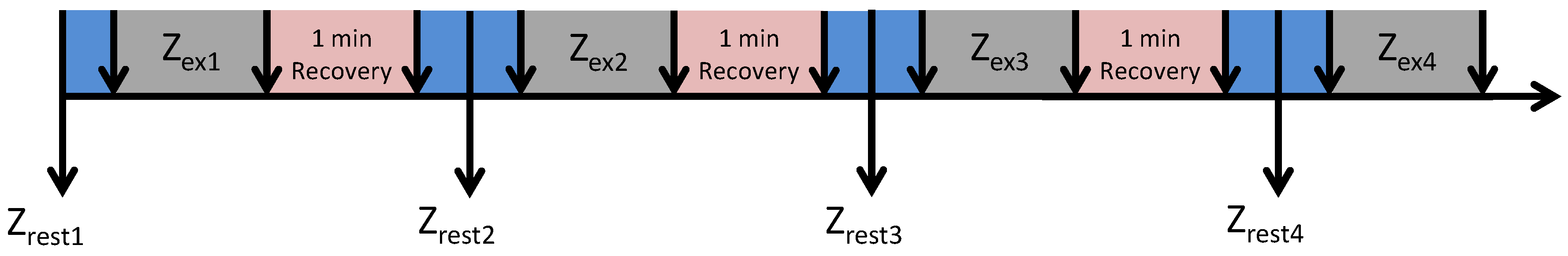
- Measure during rest state (mean of 40 spectra),
- Measure during exercise () (250 spectra),
- Rest (1 min),
- Repeat the items above three more times.
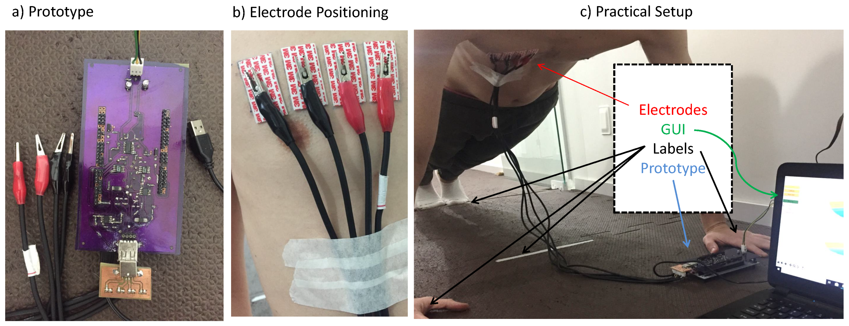
3. Prototype Design
3.1. DIBS
3.2. System Concept
3.3. Current Source
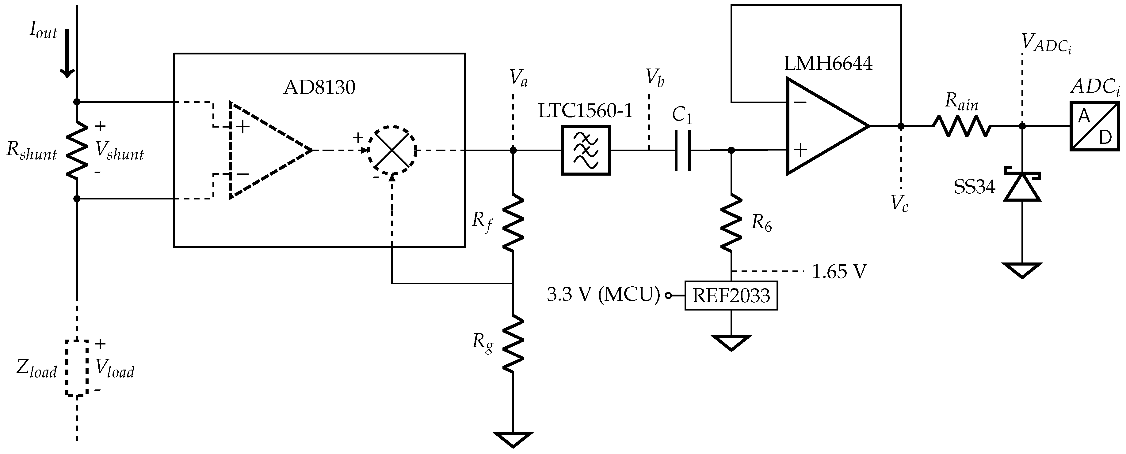
3.4. Current Acquisition
3.4.1. , and
3.4.2. Filtering and Offset
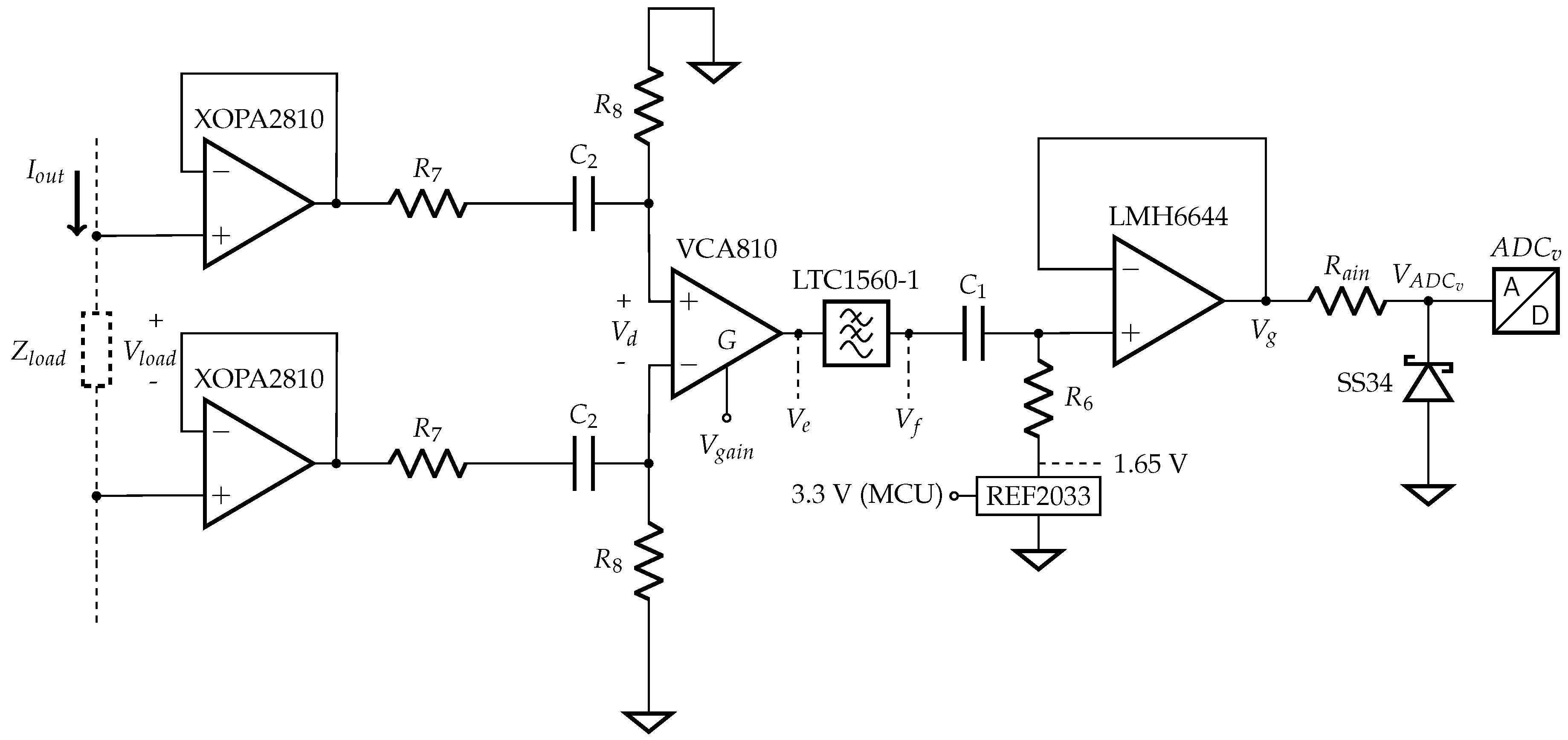
3.5. Voltage Acquisition
3.5.1. Buffer and
3.5.2. and
3.5.3. Filtering and Offset
3.6. Firmware
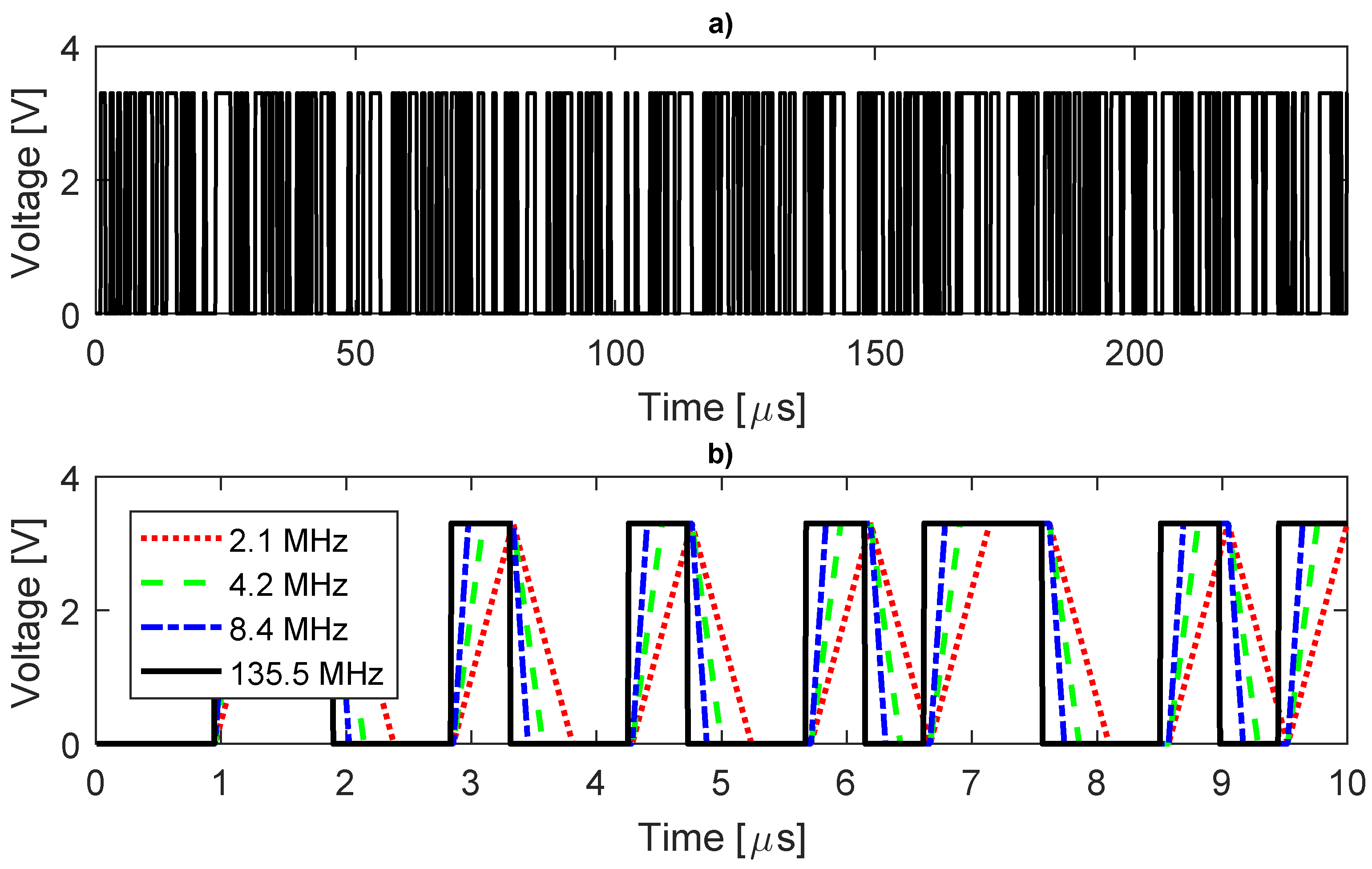
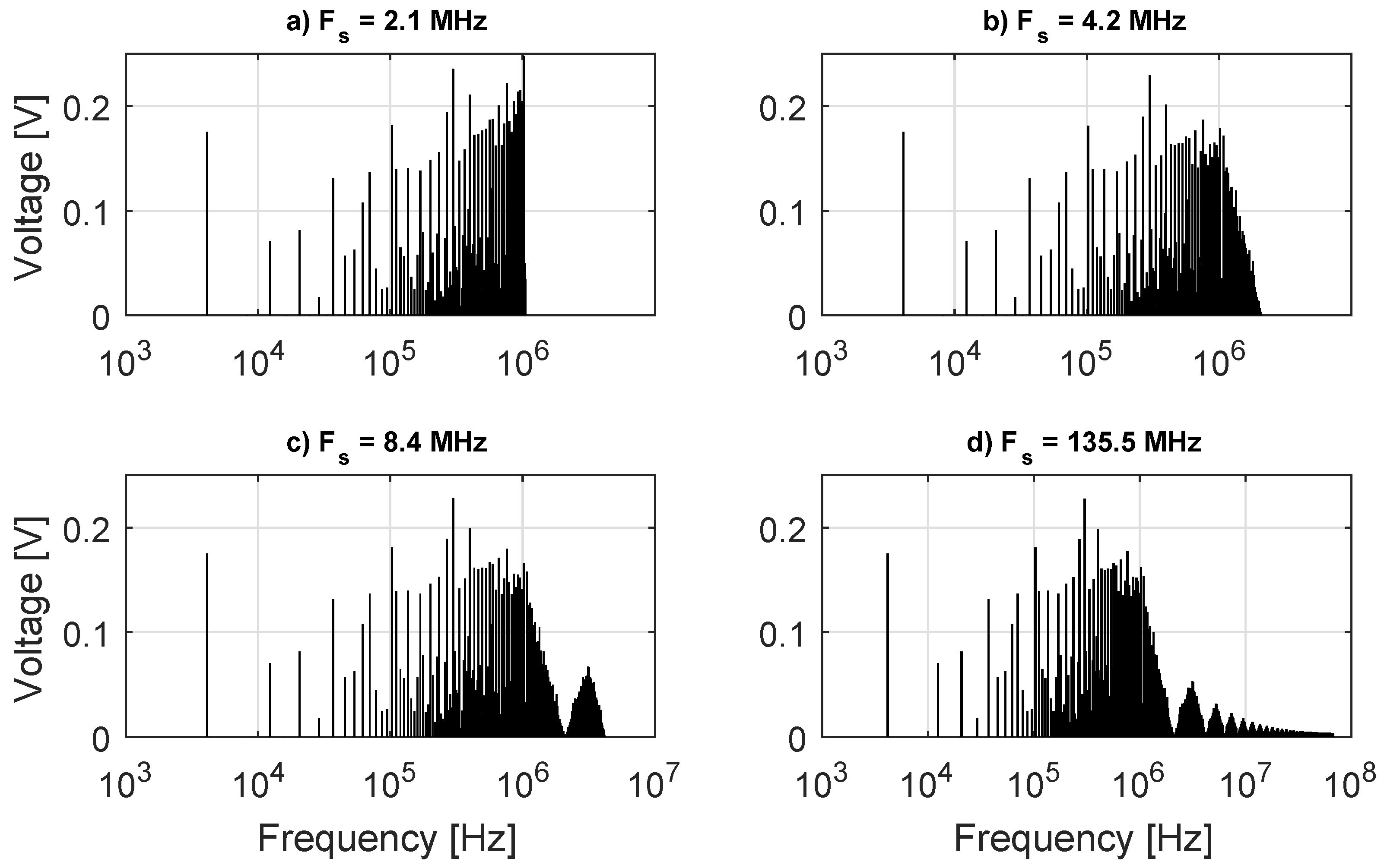
3.6.1. Signal Generation
3.6.2. Data Acquisition
3.6.3. Communication
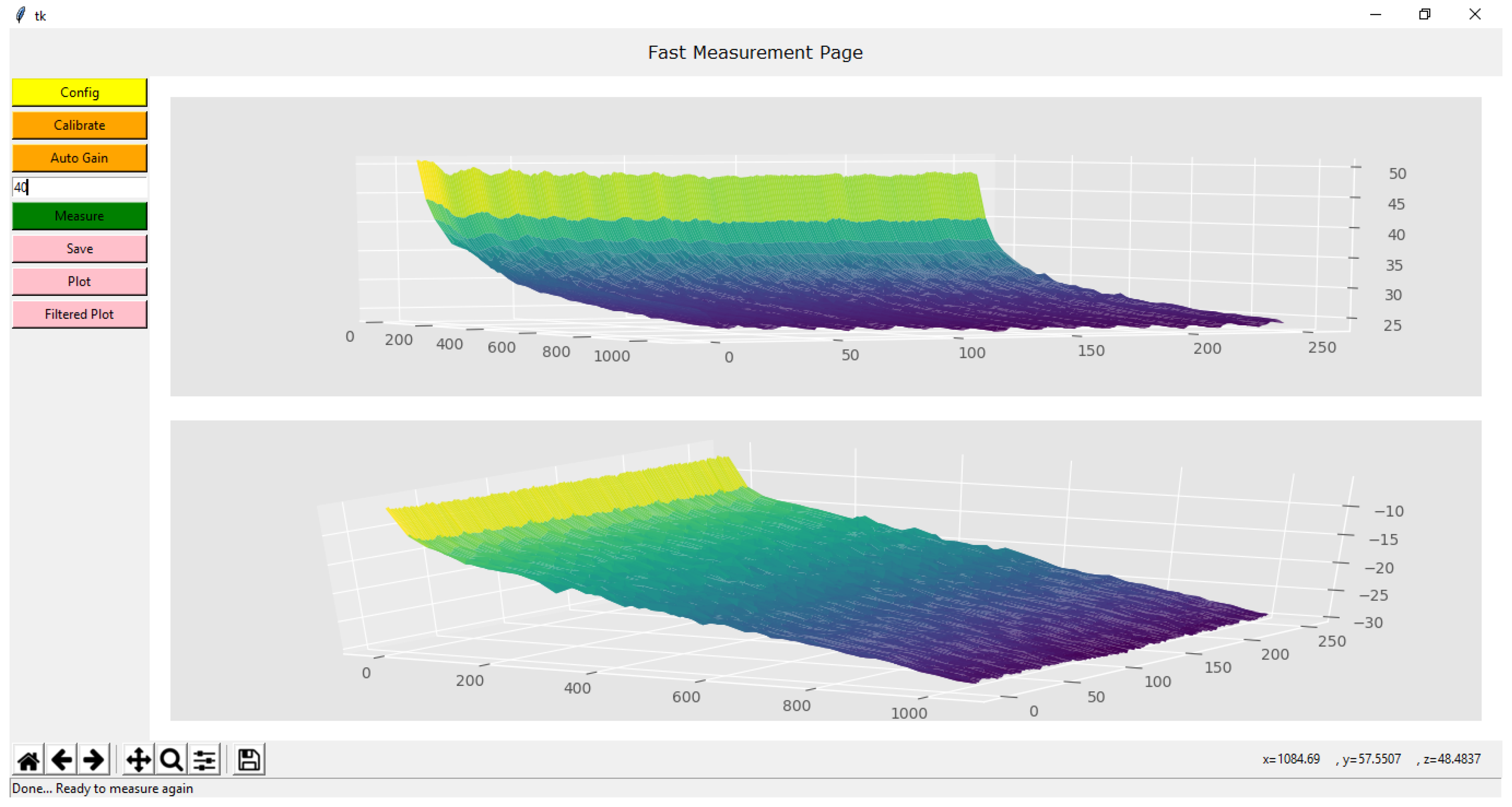
3.7. GUI
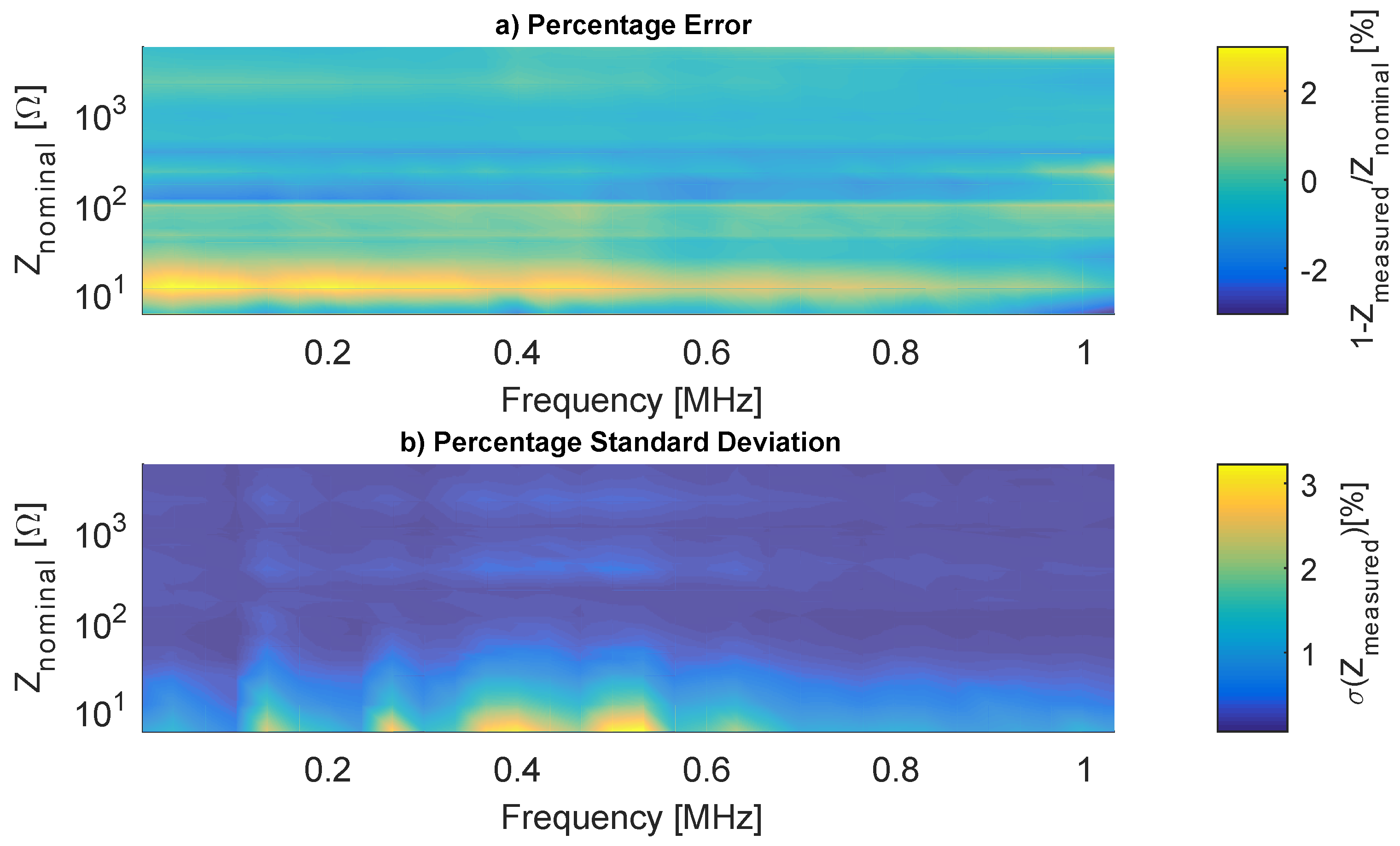
3.8. Instrument Characterization
4. Results
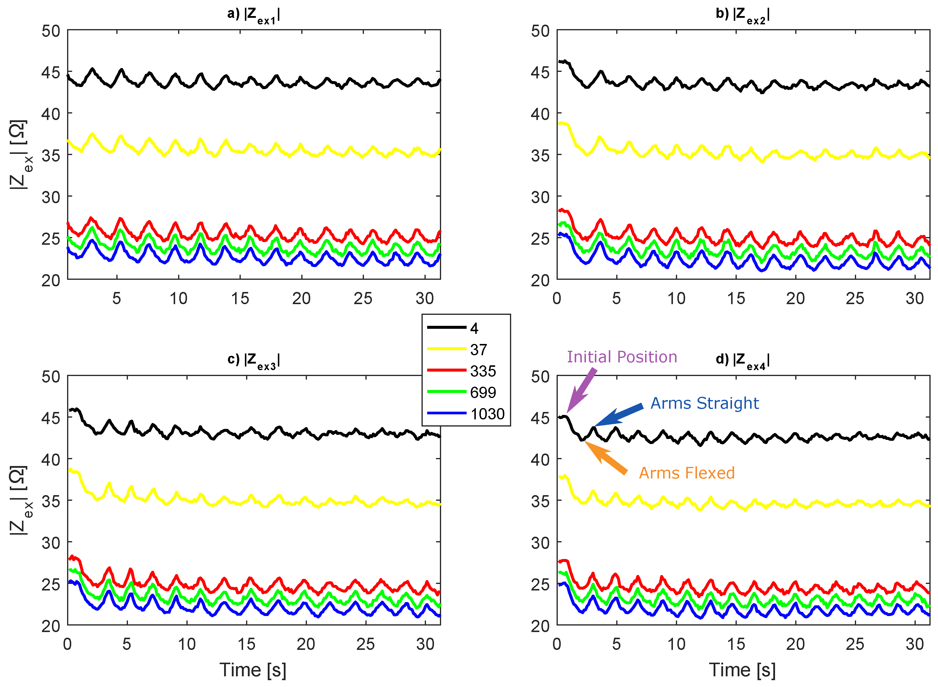
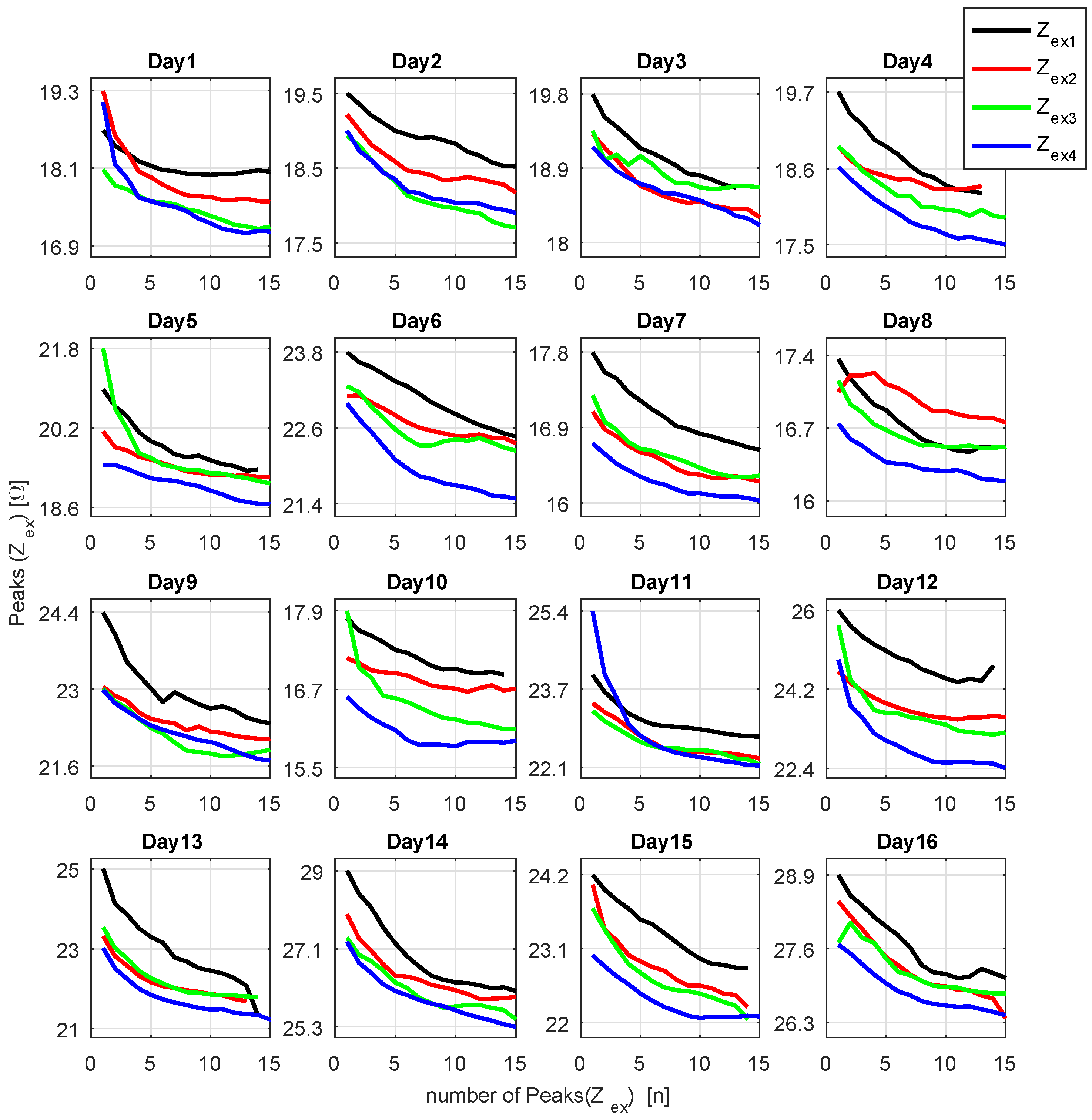
4.1. Analysis of
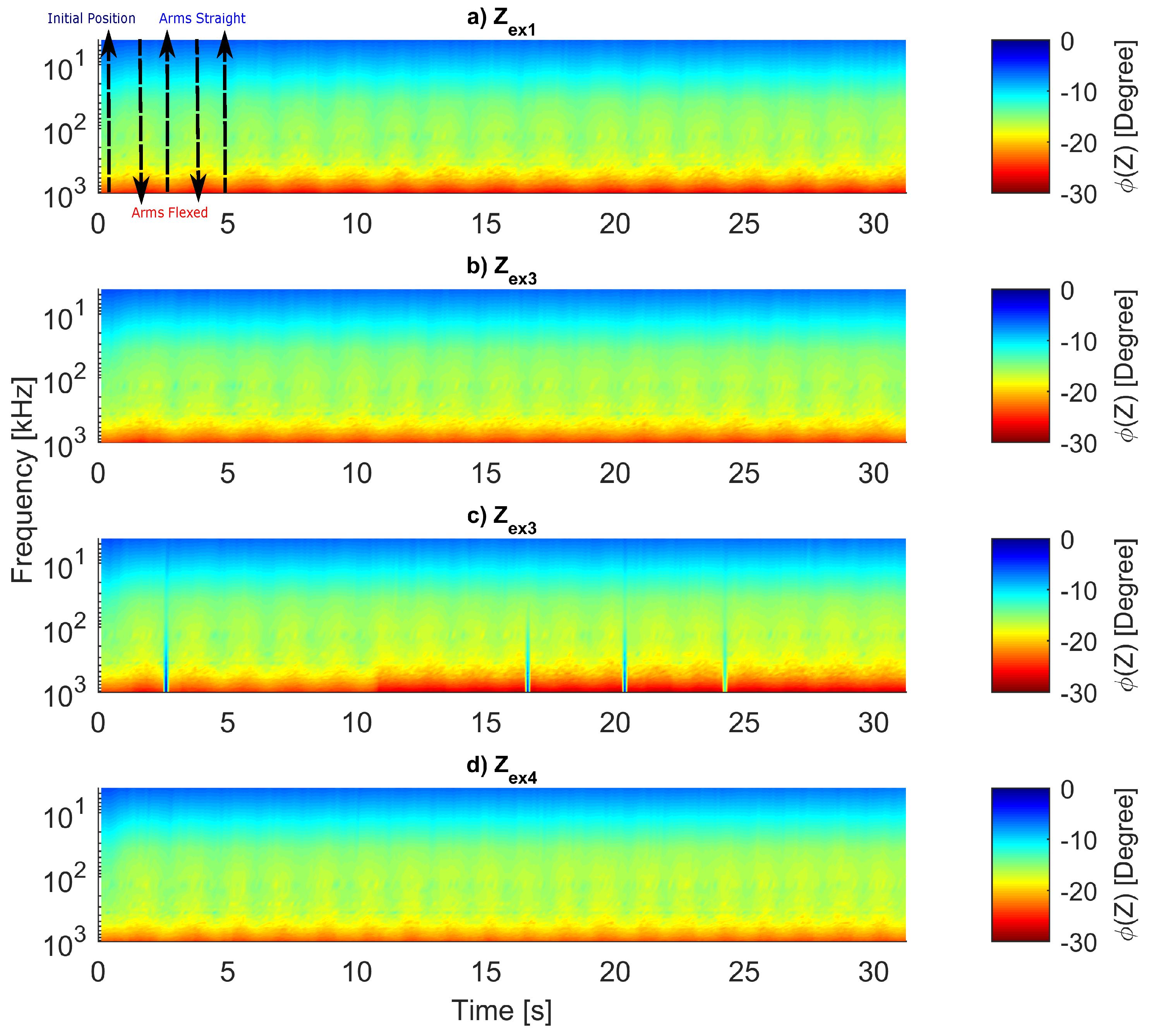
4.2. Analysis of
5. Discussion
6. Conclusions
Author Contributions
Funding
Acknowledgments
Conflicts of Interest
Abbreviations
| MUT | Material Under Test |
| EBIS | Electrical Bioimpedance Spectroscopy |
| EBIM | Electrical Bioimpedance Myography |
| DIBS | Discrete Interval Binary Sequences |
| Impedance measured during exercise | |
| Impedance measured during rest (Mean of 40 spectra) | |
| φ | Phase angle of |
| TC | Tiredness Coefficient |
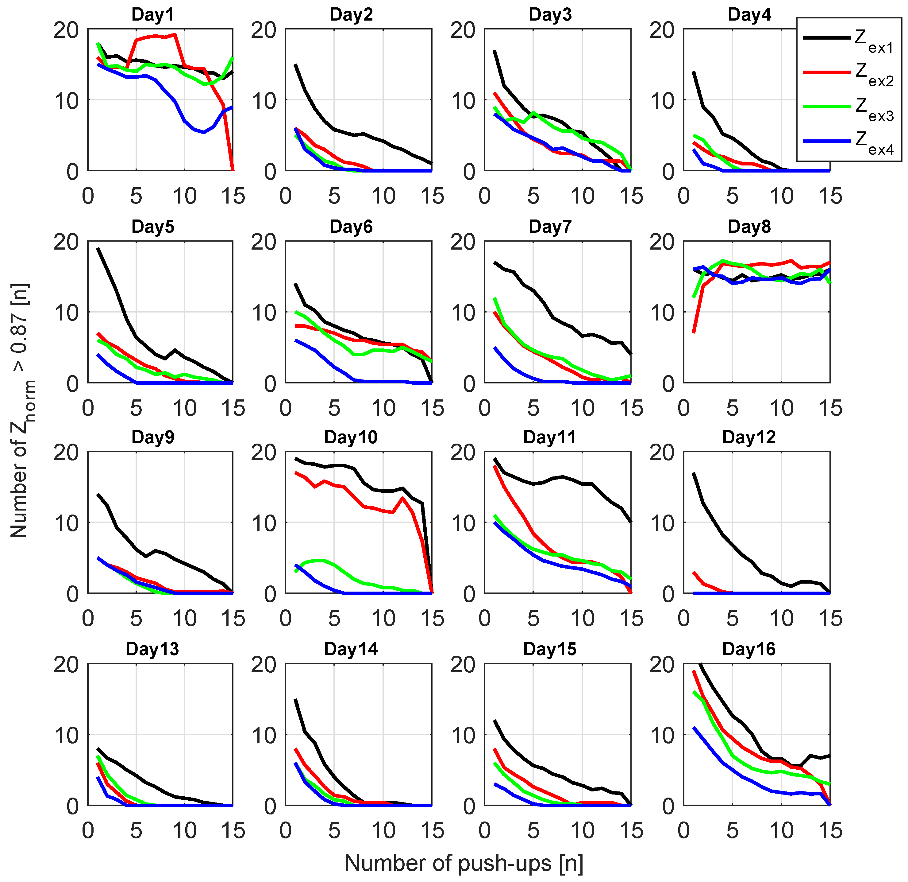
| ZnGTC | number of Greater than the Tiredness Coefficient |
References
- Grimnes, S.; Martinsen, Ø.G. Bioimpedance and Bioelectricity Basics, 2nd ed.; Elsevier Ltd.: Amsterdam, The Netherlands, 2008; p. 488. [Google Scholar]
- Buendía Lopez, R. Improvements in Bioimpedance Spectroscopy Data Analysis: Artefact Correction, Cole Parameters, and Body Fluid Estimation. Ph.D. Thesis, KTH—Royal Institute of Technology and University of Alcalá, Stockholm, Sweden, 2013. [Google Scholar]
- Gouaux, E.; MacKinnon, R. Principles of selective ion transport in channels and pumps. Science 2005, 310, 1461–1465. [Google Scholar] [CrossRef] [PubMed]
- Abtahi, F. Aspects of Electrical Bioimpedance Spectrum Estimation. Ph.D. Thesis, KTH, Stockholm, Sweden, 2014. [Google Scholar]
- Bera, T.K. Bioelectrical Impedance Methods for Noninvasive Health Monitoring: A review. J. Med. Eng. 2013, 2014, 381251. [Google Scholar] [CrossRef]
- Atefi, S.R. Electrical Bioimpedance Cerebral Monitoring: From Hypothesis and Simulation to First Experimental Evidence in Stroke Patients. Ph.D. Thesis, Royal Institute of Technology KTH, Stockholm, Sweden, 2007. [Google Scholar] [CrossRef]
- Srinivasaraghavan, V. Bioimpedance Spectroscopy of Breast Cancer Cells: A Microsystems Approach. Ph.D. Thesis, Virginia Tech, Blacksburg, VA, USA, 18 September 2015. [Google Scholar]
- Perez-Garcia, P.; Maldonado, A.; Yufera, A.; Huertas, G.; Rueda, A.; Huertas, J.L. Towards Bio-Impedance Based Labs: A Review. In Proceedings of the 2015 Conference on Design of Circuits and Integrated Systems (DCIS 2015), Estoril, Portugal, 25–27 November 2015; pp. 1–5. [Google Scholar] [CrossRef]
- Martens, O.; Land, R.; Min, M.; Annus, P.; Rist, M.; Reidla, M. Improved impedance analyzer with binary excitation signals. In Proceedings of the IEEE International Symposium on Intelligent Signal Processing (WISP 2015), Siena, Italy, 15–17 May 2015. [Google Scholar] [CrossRef]
- Bertemes-Filho, P. Tissue Characterisation using an Impedance Spectroscopy Probe. Ph.D. Thesis, University of Sheffield, Sheffield, UK, 2002. [Google Scholar]
- Min, M.; Paavle, T.; Annus, P.; Land, R. Rectangular wave excitation in wideband bioimpedance spectroscopy. In Proceedings of the 2009 IEEE International Workshop on Medical Measurements and Applications (MeMeA 2009), Cetraro, Italy, 29–30 May 2009; pp. 268–271. [Google Scholar] [CrossRef]
- Min, M.; Ojarand, J.; Martens, O.; Paavle, T.; Land, R.; Annus, P.; Rist, M.; Reidla, M.; Parve, T. Binary signals in impedance spectroscopy. In Proceedings of the 2012 Annual International Conference of the IEEE Engineering in Medicine and Biology Society (EMBS), San Diego, CA, USA, 28 August–1 September 2012; pp. 134–137. [Google Scholar] [CrossRef]
- Degen, T.; Jäckel, H. Continuous monitoring of electrode—Skin impedance mismatch during bioelectric recordings. IEEE Trans. Biomed. Eng. 2008, 55, 1711–1715. [Google Scholar] [CrossRef]
- Sanchez, B.; Vandersteen, G.; Bragos, R.; Schoukens, J. Basics of broadband impedance spectroscopy measurements using periodic excitations. Meas. Sci. Technol. 2012, 23, 105501. [Google Scholar] [CrossRef]
- Godfrey, K.R.; Tan, A.H.; Barker, H.A.; Chong, B. A survey of readily accessible perturbation signals for system identification in the frequency domain. Control Eng. Pract. 2005, 13, 1391–1402. [Google Scholar] [CrossRef]
- Ojarand, J.; Rist, M.; Min, M. Comparison of excitation signals and methods for a wideband bioimpedance measurement. In Proceedings of the 2016 IEEE International Instrumentation and Measurement Technology Conference Proceedings, Taipei, Taiwan, 23–26 May 2016. [Google Scholar] [CrossRef]
- Ojarand, J.; Min, M.; Annus, P. Crest factor optimization of the multisine waveform for bioimpedance spectroscopy. Physiol. Meas. 2014, 35, 1019–1033. [Google Scholar] [CrossRef] [PubMed]
- Land, R.; Cahill, B.P.; Parve, T.; Annus, P.; Min, M. Improvements in design of spectra of multisine and binary excitation signals for multi-frequency bioimpedance measurement. In Proceedings of the Annual International Conference of the IEEE Engineering in Medicine and Biology Society (EMBS), Boston, MA, USA, 30 August–3 September 2011; pp. 4038–4041. [Google Scholar] [CrossRef]
- Ojarand, J.; Annus, P.; Min, M.; Gorev, M.; Ellervee, P. Optimization of multisine excitation for a bioimpedance measurement device. In Proceedings of the 2014 IEEE International Instrumentation and Measurement Technology Conference (I2MTC) Proceedings, Montevideo, Uruguay, 12–15 May 2014; pp. 829–832. [Google Scholar] [CrossRef]
- Ojarand, J.; Land, R.; Min, M. Comparison of spectrally sparse excitation signals for fast bioimpedance spectroscopy: In the context of cytometry. In Proceedings of the 2012 IEEE Symposium on Medical Measurements and Applications Proceedings (MeMeA 2012), Budapest, Hungary, 18–19 May 2012; pp. 214–218. [Google Scholar] [CrossRef]
- Rutkove, S.B. Electrical impedance myography: Background, current state, and future directions. Muscle Nerve 2009, 40, 936–946. [Google Scholar] [CrossRef] [Green Version]
- Li, X.; Li, L.; Shin, H.; Li, S.; Zhou, P. Electrical impedance myography for evaluating paretic muscle changes after stroke. IEEE Trans. Neural Syst. Rehabil. Eng. 2017, 25, 2113–2121. [Google Scholar] [CrossRef]
- Rutkove, S.B.; Pacheck, A.; Sanchez, B. Sensitivity distribution simulations of surface electrode configurations for electrical impedance myography. Muscle Nerve 2017, 56, 887–895. [Google Scholar] [CrossRef]
- Clemente, F.; Romano, M.; Bifulco, P.; Cesarelli, M. Study of muscular tissue in different physiological conditions using electrical impedance spectroscopy measurements. Biocybern. Biomed. Eng. 2014, 34, 4–9. [Google Scholar] [CrossRef]
- Fu, B.; Freeborn, T.J. Biceps tissue bioimpedance changes from isotonic exercise-induced fatigue at different intensities. Biomed. Phys. Eng. Express 2018, 4, 025037. [Google Scholar] [CrossRef] [Green Version]
- Freeborn, T.J.; Bohannan, G.W. Changes of Fractional-Order Model Parameters in Biceps Tissue from Fatiguing Exercise. In Proceedings of the 2018 IEEE International Symposium on Circuits and Systems (ISCAS), Florence, Italy, 27–30 May 2018; pp. 1–5. [Google Scholar] [CrossRef]
- Li, L.; Shin, H.; Li, X.; Li, S.; Zhou, P. Localized electrical impedance myography of the biceps brachii muscle during different levels of isometric contraction and fatigue. Sensors 2016, 16, 581. [Google Scholar] [CrossRef]
- Harrison, A.P.; Elbrønd, V.S.; Riis-Olesen, K.; Bartels, E.M. Multi-frequency bioimpedance in equine muscle assessment. Physiol. Meas. 2015, 36, 453–464. [Google Scholar] [CrossRef] [PubMed]
- Son, C.; Kim, S.; Jong Kim, S.; Choi, J.; Kim, D.E. Detection of muscle activation through multi-electrode sensing using electrical stimulation. Sens. Actuators A Phys. 2018, 275, 19–28. [Google Scholar] [CrossRef]
- Nescolarde, L.; Yanguas, J.; Lukaski, H.; Alomar, X.; Rosell-Ferrer, J.; Rodas, G. Effects of muscle injury severity on localized bioimpedance measurements. Physiol. Meas. 2015, 36, 27–42. [Google Scholar] [CrossRef] [PubMed]
- Sanchez, B.; Iyer, S.R.; Li, J.; Kapur, K.; Xu, S.; Rutkove, S.B.; Lovering, R.M. Non-invasive assessment of muscle injury in healthy and dystrophic animals with electrical impedance myography. Muscle Nerve 2017, 56, E85–E94. [Google Scholar] [CrossRef] [PubMed]
- Sanchez, B.; Pacheck, A.; Rutkove, S.B. Guidelines to electrode positioning for human and animal electrical impedance myography research. Sci. Rep. 2016, 6, 32615. [Google Scholar] [CrossRef] [PubMed] [Green Version]
- Ibrahim, B.; Hall, D.A.; Jafari, R. Bio-impedance spectroscopy (BIS) measurement system for wearable devices. In Proceedings of the 2017 IEEE Biomedical Circuits and Systems Conference (BioCAS), Torino, Italy, 19–21 October 2017; pp. 1–4. [Google Scholar] [CrossRef]
- Kwon, H.; Rutkove, S.B.; Sanchez, B. Recording characteristics of electrical impedance myography needle electrodes. Physiol. Meas. 2017, 38, 1748–1765. [Google Scholar] [CrossRef]
- Sirtoli, V.G. Desenvolvimento de um Medidor de Bioimpedância Rápido Utilizando Discrete Interval Binary Sequences (DIBS). Master’s Thesis, Universidade do Estado de Santa Catarina, Joinville, Brazil, 2018. [Google Scholar] [CrossRef]
- Tucker, A.S.; Fox, R.M.; Sadleir, R.J. Biocompatible, high precision, wideband, improved howland current source with lead-lag compensation. IEEE Trans. Biomed. Circuits Syst. 2013, 7, 63–70. [Google Scholar] [CrossRef]
- Hong, H.; Rahal, M.; Demosthenous, A.; Bayford, R.H. Comparison of a new integrated current source with the modified howland circuit for EIT applications. Physiol. Meas. 2009, 30, 999. [Google Scholar] [CrossRef]
- Morcelles, K.F.; Sirtoli, V.G.; Bertemes-Filho, P.; Vincence, V.C. Howland current source for high impedance load applications. Rev. Sci. Instrum. 2017, 88, 114705. [Google Scholar] [CrossRef] [PubMed]
- Filho, P.B.; Lima, R.G.; Tanaka, H. A current source using a negative impedance converter (NIC) for electrical impedance tomography (EIT). In Proceedings of the 17th International Congress of Mechanical Engineering, São Paulo, SP, Brazil, 10–14 November 2003. [Google Scholar]
- Qureshi, T.R.; Chatwin, C.R.; Huber, N.; Zarafshani, A.; Tunstall, B.; Wang, W. Comparison of Howland and General Impedance Converter (GIC) circuit based current sources for bio-impedance measurements. J. Phys. Conf. Ser. 2010, 224, 012167. [Google Scholar] [CrossRef] [Green Version]
- Pliquett, U.; Schönfeldt, M.; Barthel, A.; Frense, D.; Nacke, T. Offset-free bidirectional current source for impedance measurement. J. Phys. Conf. Ser. 2010, 224, 012009. [Google Scholar] [CrossRef] [Green Version]
- Rosa, B.M.; Yang, G.Z. Smart wireless headphone for cardiovascular and stress monitoring. In Proceedings of the 2017 IEEE 14th International Conference on Wearable and Implantable Body Sensor Networks (BSN 2017), Eindhoven, The Netherlands, 9–12 May 2017. [Google Scholar] [CrossRef]
- Sirtoli, V.G.; Morcelles, K.F.; Vincence, V.C. Design of current sources for load common mode optimization. J. Electr. Bioimpedance 2018, in press. [Google Scholar] [CrossRef]
- Kassanos, P.; Constantinou, L.; Triantis, I.F.; Demosthenous, A. An integrated analog readout for multi-frequency bioimpedance measurements. IEEE Sens. J. 2014, 14, 2792–2800. [Google Scholar] [CrossRef]
- Langlois, P.J.; Neshatvar, N.; Demosthenous, A. A sinusoidal current driver with an extended frequency range and multifrequency operation for bioimpedance applications. IEEE Trans. Biomed. Circuits Syst. 2015, 9, 401–411. [Google Scholar] [CrossRef] [PubMed]
- Kassanos, P.; Yang, G.Z. A CMOS programmable phase shifter for compensating synchronous detection bioimpedance systems. In Proceedings of the 2017 24th IEEE International Conference on Electronics, Circuits and Systems (ICECS), Batumi, Georgia, 5–8 December 2017; pp. 218–221. [Google Scholar] [CrossRef]
- Kusche, R.; Malhotra, A.; Ryschka, M.; Ardelt, G.; Klimach, P.; Kaufmann, S. A FPGA-Based Broadband EIT System for Complex Bioimpedance Measurements—Design and Performance Estimation. Electronics 2015, 4, 507. [Google Scholar] [CrossRef]
- Enoka, R.M.; Stuart, D.G. Neurobiology of muscle fatigue. J. Appl. Physiol. 1992, 72, 1631–1648. [Google Scholar] [CrossRef]


© 2018 by the authors. Licensee MDPI, Basel, Switzerland. This article is an open access article distributed under the terms and conditions of the Creative Commons Attribution (CC BY) license (http://creativecommons.org/licenses/by/4.0/).
Share and Cite
Sirtoli, V.; Morcelles, K.; Gomez, J.; Bertemes-Filho, P. Design and Evaluation of an Electrical Bioimpedance Device Based on DIBS for Myography during Isotonic Exercises. J. Low Power Electron. Appl. 2018, 8, 50. https://0-doi-org.brum.beds.ac.uk/10.3390/jlpea8040050
Sirtoli V, Morcelles K, Gomez J, Bertemes-Filho P. Design and Evaluation of an Electrical Bioimpedance Device Based on DIBS for Myography during Isotonic Exercises. Journal of Low Power Electronics and Applications. 2018; 8(4):50. https://0-doi-org.brum.beds.ac.uk/10.3390/jlpea8040050
Chicago/Turabian StyleSirtoli, Vinicius, Kaue Morcelles, John Gomez, and Pedro Bertemes-Filho. 2018. "Design and Evaluation of an Electrical Bioimpedance Device Based on DIBS for Myography during Isotonic Exercises" Journal of Low Power Electronics and Applications 8, no. 4: 50. https://0-doi-org.brum.beds.ac.uk/10.3390/jlpea8040050