A Short-Time Repeat TLS Survey to Estimate Rates of Glacier Retreat and Patterns of Forefield Development (Case Study: Scottbreen, SW Svalbard)


Abstract
:1. Introduction
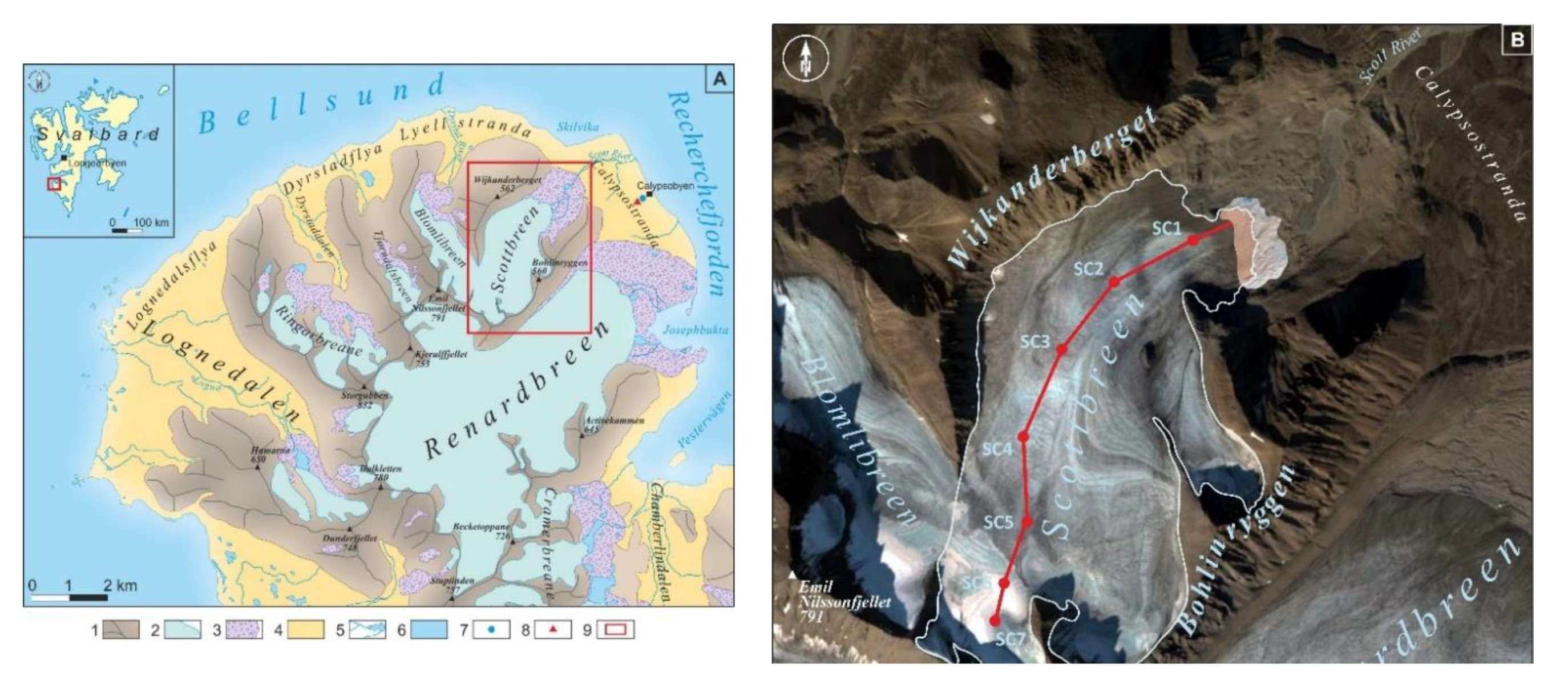
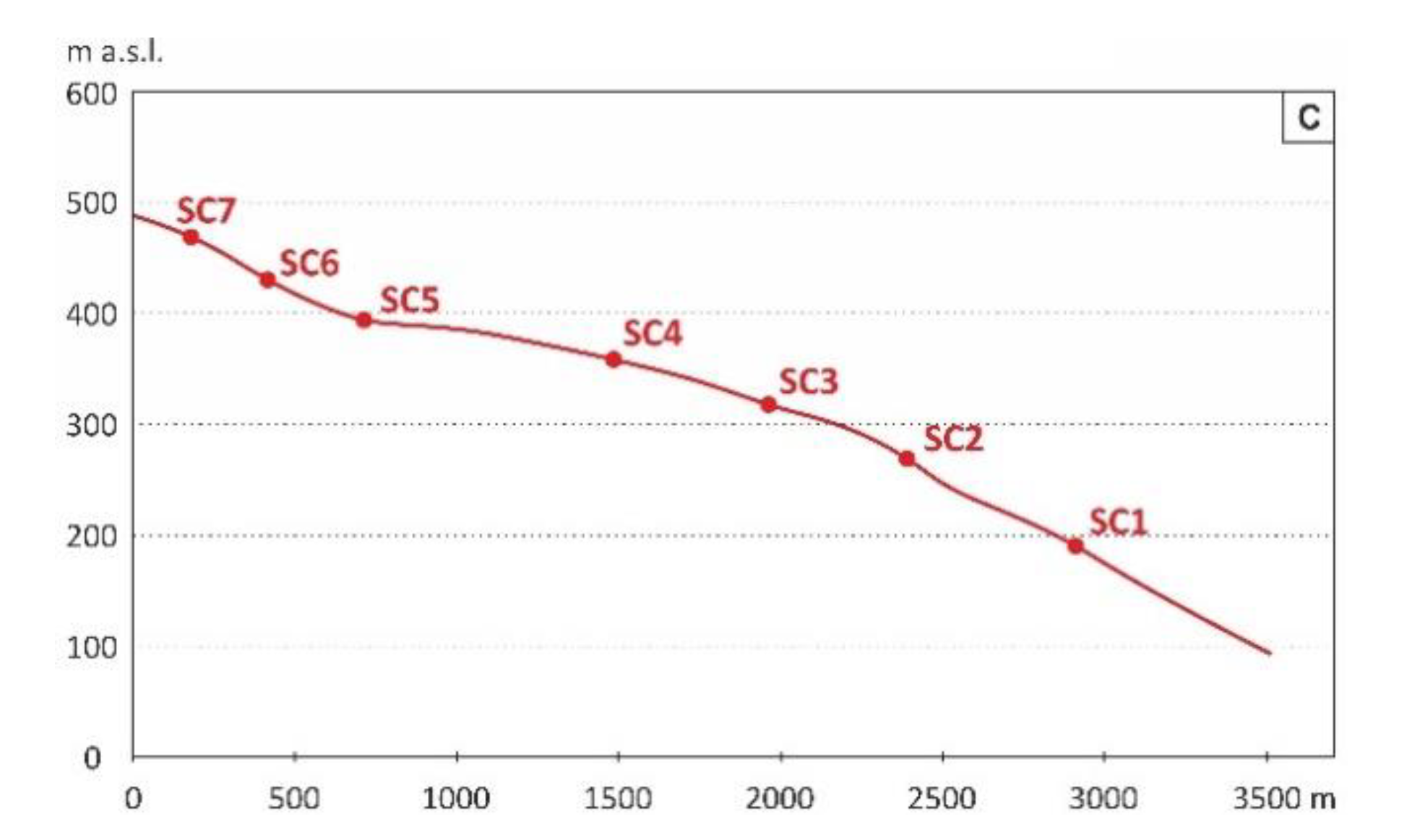
2. Study Area
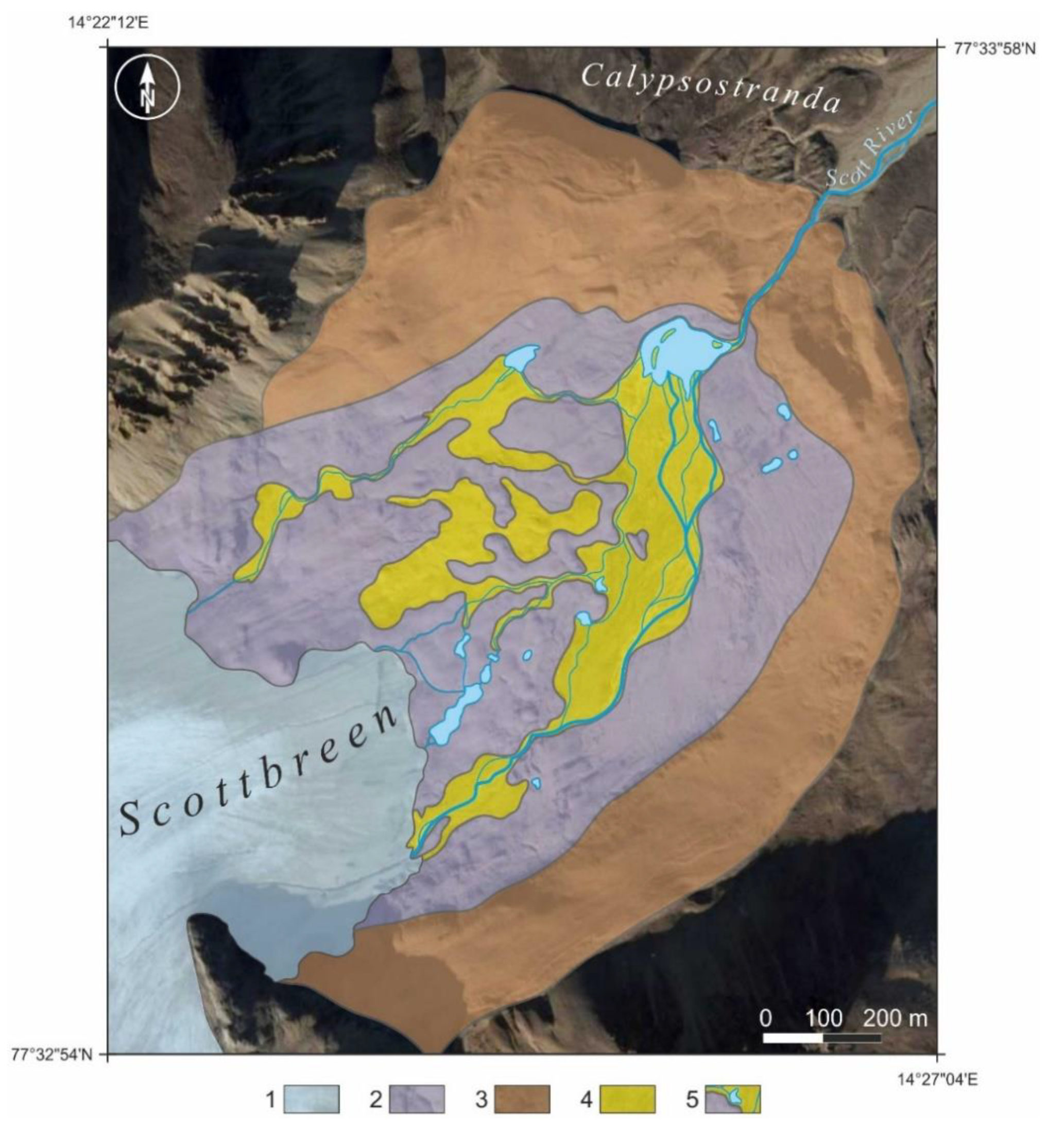
Geomorphology
3. Methods
3.1. Data Acquisition. TLS and rtkGPS Surveys
3.2. DEM Parameters and Data Analysis
3.3. Meteorological Measurements
3.4. Direct Glaciological Measurements
4. Results
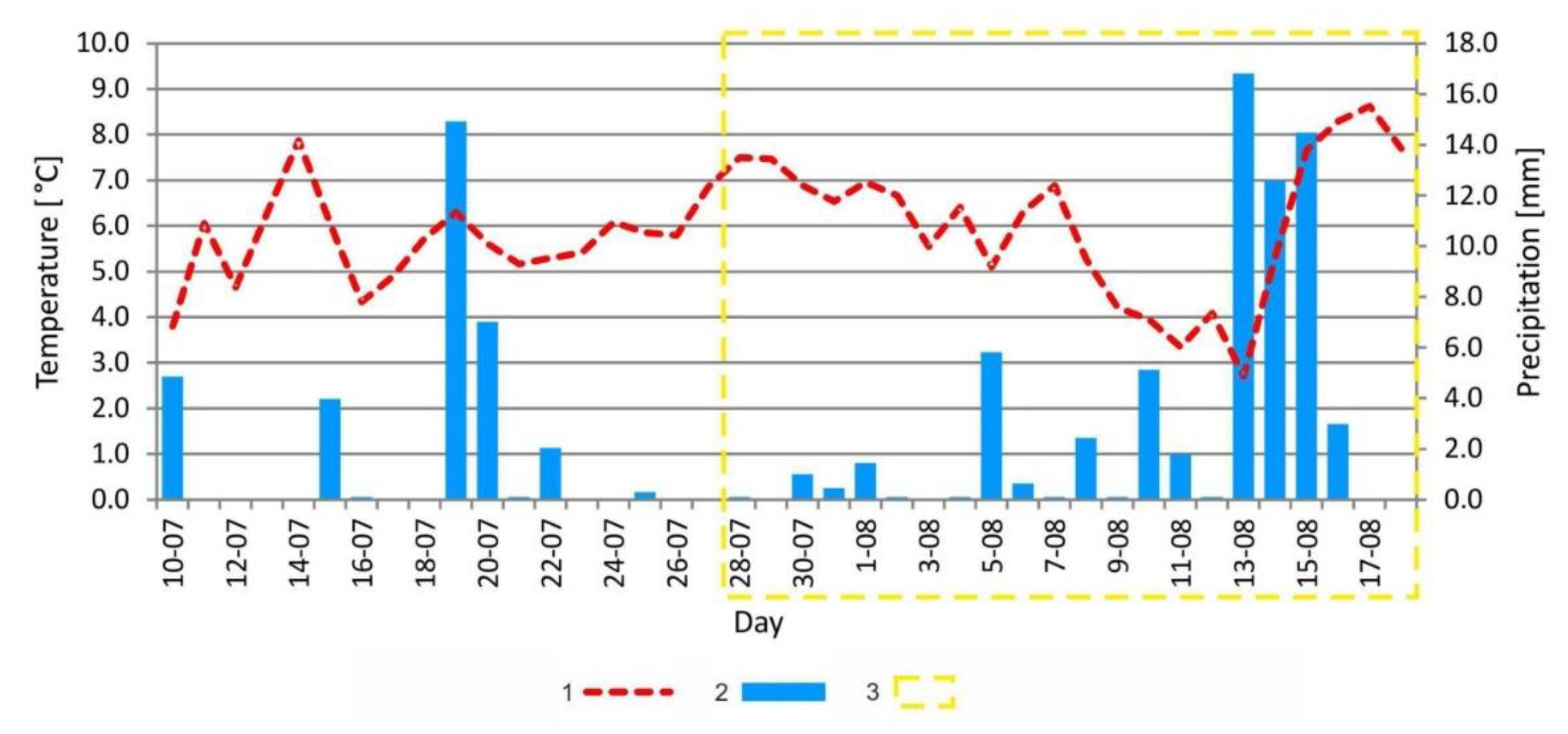
4.1. Meteorological Conditions
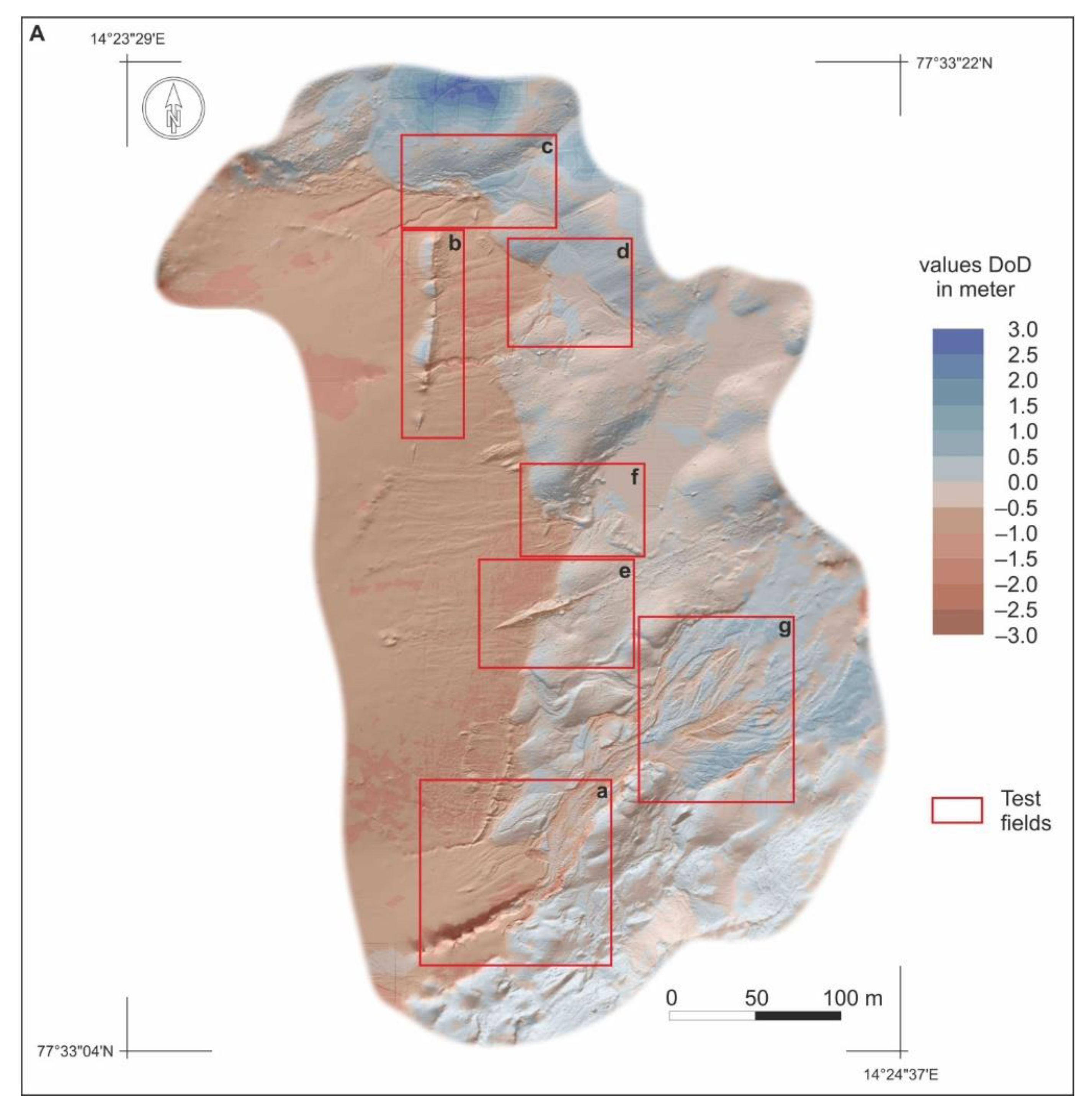
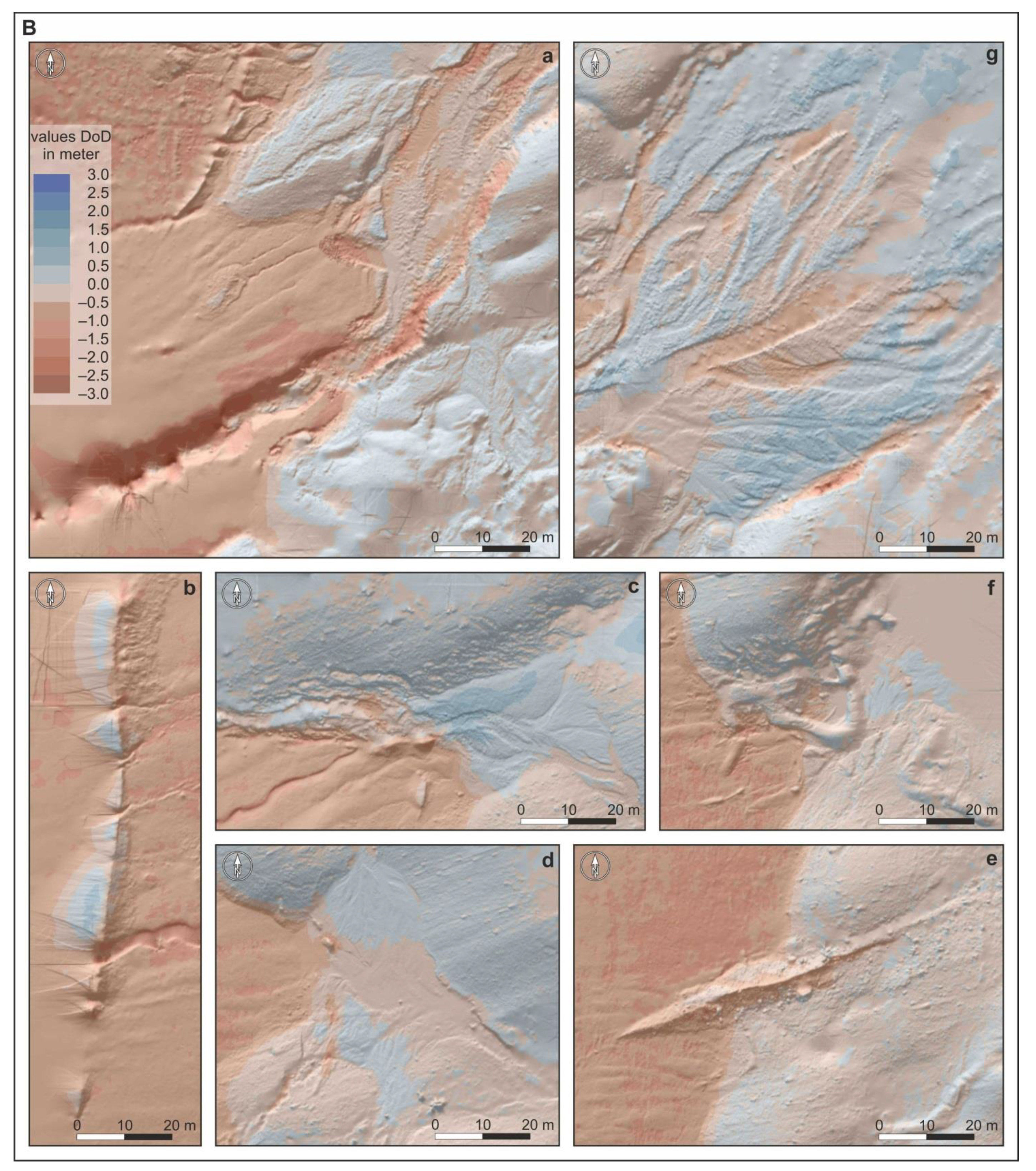
4.2. Geomorphic Change Detection Analysis by TLS-Based DEMs
4.3. Morphological Changes
4.3.1. Glacier Zone (Clear Ice Zone)
4.3.2. Recently-Deglaciated Area (Zone)
4.3.3. Glacier Forefield—Inner Marginal Zone
5. Discussion
6. Conclusions
- The foreland of the Scottbreen—a typical valley glacier that has undergone dynamic transformations connected with its terminus, which in turn have retreated at a rate of 22 m year−1—makes up an interesting research study into the contemporary development of newly deglaciated areas. Comparative measurements in the 3-week period at the turn of July and August of 2013 introduce a new quality into spatial analyses of glacial areas. They have made it possible to perform quantitative and qualitative evaluations on the range and direction of landform development. The spatial analysis on the dynamics of geomorphic processes that shape said zone has given rise to tracing short-term landform transformations under conditions of progressive degradation of the glacial catchment’s cryosphere in the sensitive High-Arctic environment.
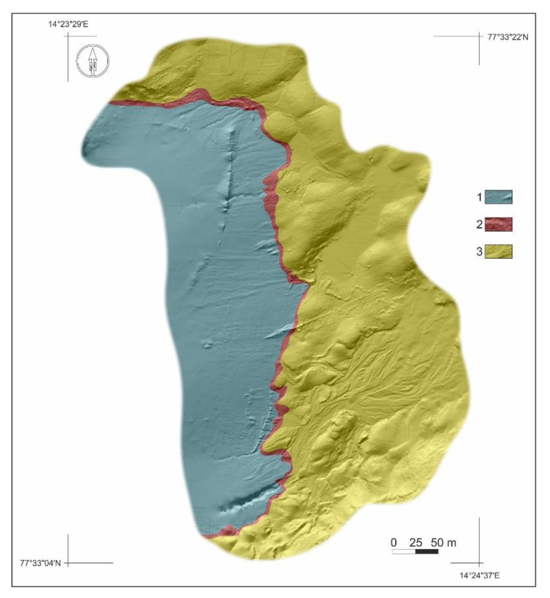
- Three zones were distinguished with respect to the differences in the dynamics of geomorphological processes: (i) the glacier front zone, which is characterised by a glacier surface lowering rate of 2 m year−1; (ii) the recently deglaciated zone with dynamic geomorphic processes, which worsens during extreme and above-average meteorological events (e.g., heavy rainfall, rapid increase in air temperature); and (iii) the inner marginal zone, which is relatively stable and characterised by an erosion/deposition balance.
- The range of transportation of supraglacial debris is limited. The majority of newly provided debris that comes from the glacier’s ablation is deposited in a narrow, recently deglaciated zone (up to 12 m). Here, a predominance of aggradation was registered in the analysed 3-week period. Moreover, redeposition of sediments into the inner marginal zone is restricted by a range of hills in the terminus and lateral moraines located at the foot of the zone, which includes numerous intramoraine fluvial basins (or, less frequently, basins that are not drained by any outflow) catching the supraglacial debris. However, during the period of above-average floods, the scree deposited in the basins may be channelled to the basins’ lower parts where it overbuilds the landform of the inner marginal outwash plain.
- It has been shown that in a very short timescale, rapid meteorological phenomena can result in relief changes that are diametrically different from the rates and directions of annual and perennial changes. The occurrence of events characterised as above-average, i.e., high precipitation and an increase in temperature during the 3-week comparative period (July–August 2013), cause the glacier’s area to lower by up to 3.5 m—this is nearly two times more than the annual mean (2 m year−1) in the 2010–2013 period.
- The conducted analysis on the dynamics of spatial changes in the proglacial zone may contribute to a better understanding of the way modern processes shape the forefield of the glacier’s terminus. Detailed comparative analyses confirmed the high precision and efficiency of high-resolution TLS-based DEM as a tool for inventorying and tracking high-dynamic development of glacial and proglacial landforms. This tool is particularly useful in analysing ephemeral landforms (from several days to several weeks long). This study’s adopted methodology for performing both measurements and comparative analyses on high-resolution models of investigated areas is far more universal and effective than methods that have been traditionally used in glaciology. Consequently, the amount of data provided during a single measurement cycle and the comparability of the findings should be the basis for implementing the TLS-based DEM analysis as a standard tool in a new comprehensive approach to conducting glaciological and geomorphological research into glacier forefields.
Author Contributions
Funding
Institutional Review Board Statement
Informed Consent Statement
Data Availability Statement
Acknowledgments
Conflicts of Interest
Appendix A

| Attribute | Raw | Thresholded DoD Estimate: | ||
|---|---|---|---|---|
| Areal Metrics | ||||
| Total Area of Surface Lowering (m2) | 143,326 | 108,948 | ||
| Total Area of Surface Raising (m2) | 62,063 | 42,225 | ||
| Total Area (m2) | 205,389 | 151,173 | 74% | |
| Total Volumetric Metrics | ± Error Volume | % Error | ||
| Total Volume of Surface Lowering (m3) | 66,049 | 65,647 | ±3082 | 5% |
| Total Volume of Surface Raising (m3) | 17,945 | 17,741 | ±1194 | 7% |
| Total Volume of Difference (m3) | 83,994 | 83,388 | ±4276 | 5% |
| Total Net Volume Difference (m3) | −48,103 | −47,905 | ±3305 | −7% |
| Vertical Averages: | ||||
| Average Depth of Surface Lowering (m) | 0.46 | 0.60 | ±0.03 | 5% |
| Average Depth of Surface Raising (m) | 0.29 | 0.42 | ±0.03 | 7% |
| Average Total Thickness of Difference (m) for Area of Interest | 0.41 | 0.41 | ±0.02 | 5% |
| Average Net Thickness Difference (m) for Study Area | −0.23 | −0.23 | ±0.02 | −7% |
| Percentages (by volume) | ||||
| Percent Elevation Lowering | 79% | 79% | ||
| Percent Surface Raising | 21% | 21% | ||
| Percent Imbalance (departure from equilibrium) | −29% | −29% | ||
| Attribute | Raw | Thresholded DoD Estimate: | ||
|---|---|---|---|---|
| Areal Metrics | ||||
| Total Area of Surface Lowering (m2) | 62,558 | 62,250 | ||
| Total Area of Surface Raising (m2) | 911 | 731 | ||
| Total Area (m2) | 63,469 | 62,981 | 99% | |
| Total Volumetric Metrics | ± Error Volume | % Error | ||
| Total Volume of Surface Lowering (m3) | 53,479 | 53,475 | ±1761 | 3% |
| Total Volume of Surface Raising (m3) | 164 | 162 | ±21 | 13% |
| Total Volume of Difference (m3) | 53,643 | 53,637 | ±1781 | 3% |
| Total Net Volume Difference (m3) | −53,315 | −53,313 | ±1761 | −3% |
| Vertical Averages: | ||||
| Average Depth of Surface Lowering (m) | 0.85 | 0.86 | ±0.03 | 5% |
| Average Depth of Surface Raising (m) | 0.18 | 0.22 | ±0.03 | 7% |
| Average Total Thickness of Difference (m) for glacier terminus | 0.85 | 0.85 | ±0.02 | 5% |
| Average Net Thickness Difference (m) for Area of Interest | −0.84 | −0.84 | ±0.02 | −7% |
| Percentages (by volume) | ||||
| Percent Elevation Lowering | 79% | 79% | ||
| Percent Surface Raising | 21% | 21% | ||
| Percent Imbalance (departure from equilibrium) | −29% | −29% | ||
| Attribute | Raw | Thresholded DoD Estimate: | ||
|---|---|---|---|---|
| Areal Metrics | ||||
| Total Area of Surface Lowering (m2) | 4495 | 4302 | ||
| Total Area of Surface Raising (m2) | 356 | 247 | ||
| Total Area (m2) | 4851 | 4549 | 94% | |
| Total Volumetric Metrics | ± Error Volume | %Error | ||
| Total Volume of Surface Lowering (m3) | 2497 | 2494 | ±122 | 5% |
| Total Volume of Surface Raising (m3) | 55 | 54 | ±7 | 13% |
| Total Volume of Difference (m3) | 2552 | 2549 | ±129 | 5% |
| Total Net Volume Difference (m3) | −2441 | −2440 | ±122 | −5% |
| Vertical Averages: | ||||
| Average Depth of Surface Lowering (m) | 0.56 | 0.58 | ±0.03 | 5% |
| Average Depth of Surface Raising (m) | 0.16 | 0.22 | ±0.03 | 13% |
| Average Total Thickness of Difference (m) for Area of Interest | 0.53 | 0.53 | ±0.03 | 5% |
| Average Net Thickness Difference (m) for Recent-Deglaciated Area | −0.50 | −0.50 | ±0.03 | −5% |
| Percentages (by volume) | ||||
| Percent Elevation Lowering | 98% | 98% | ||
| Percent Surface Raising | 2% | 2% | ||
| Percent Imbalance (departure from equilibrium) | −48% | −48% | ||
| Attribute | Raw | Thresholded DoD Estimate: | ||
|---|---|---|---|---|
| Areal Metrics | ||||
| Total Area of Surface Lowering (m2) | 80,495 | 46,429 | ||
| Total Area of Surface Raising (m2) | 61,106 | 41,451 | ||
| Total Area (m2) | 141,601 | 62% | ||
| Total Volumetric Metrics | ± Error Volume | % Error | ||
| Total Volume of Surface Lowering (m3) | 12,372 | 11,974 | ±1313 | 11% |
| Total Volume of Surface Raising (m3) | 17,773 | 17,570 | ±1172 | 7% |
| Total Volume of Difference (m3) | 30,145 | 29,545 | ±2486 | 8% |
| Total Net Volume Difference (m3) | 5400 | 5596 | ±1760 | 31% |
| Vertical Averages: | ||||
| Average Depth of Surface Lowering (m) | 0.15 | 0.26 | ±0.03 | 11% |
| Average Depth of Surface Raising (m) | 0.29 | 0.42 | ±0.03 | 7% |
| Average Total Thickness of Difference (m) for Area of Interest | 0.21 | 0.21 | ±0.02 | 8% |
| Average Net Thickness Difference (m) for Glacier Forefield | 0.04 | 0.04 | ±0.01 | 31% |
| Percentages (by volume) | ||||
| Percent Elevation Lowering | 41% | 41% | ||
| Percent Surface Raising | 59% | 59% | ||
| Percent Imbalance (departure from equilibrium) | 9% | 9% | ||
References
- Hagen, J.O.; Liestøl, O.; Roland, E.; Jørgensen, T. Glacier Atlas of Svalbard and Jan Mayen; Norsk Polarinstitutt Meddelelser: Oslo, Norway, 1993; p. 141. [Google Scholar]
- Jania, J.; Hagen, J.O. Mass Balance of Arctic Glaciers; University of Silesia: Sosnowiec-Oslo, Poland, 1996; p. 62. [Google Scholar]
- Hagen, J.O.; Melvold, K.; Pinglot, F.; Dowdeswell, J.A. On the net mass balance of the glaciers and ice caps in Svalbard, Norwegian. Arct. Antarct. Alp. Res. 2003, 35, 264–270. [Google Scholar] [CrossRef] [Green Version]
- Hagen, J.O.M.; Eiken, T.; Kohler, J.; Melvold, K. Geometry changes on Svalbard glaciers: Mass-balance or dynamic response? Ann. Glaciol. 2005, 42, 255–261. [Google Scholar] [CrossRef] [Green Version]
- Błaszczyk, M.; Jania, J.A.; Hagen, J.O. Tidewater glaciers of Svalbard: Recent changes and estimates of calving fluxes. Polar Res. 2009, 30, 85–142. [Google Scholar]
- Zemp, M.; Hoelzle, M.; Haeberli, W. Six decades of glacier mass-balance observations: A re-view of the worldwide monitoring network. Ann. Glaciol. 2009, 50, 101–111. [Google Scholar] [CrossRef] [Green Version]
- Pachauri, R.K.; Meyeer, L.A. (Eds.) IPCC Climate Change 2014: Synthesis Report. In Contribution of Working Groups I, II and III to the Fifth Assessment Report of the Intergovernmental Panel on Climate Change; IPCC: Geneva, Switzerland, 2014. [Google Scholar]
- Christianson, K.; Kohler, J.; Alley, R.B.; Nuth, C.; Van Pelt, W. Dynamic perennial firn aquifer on an Arctic glacier. Geophys. Res. Lett. 2015, 42, 1418–1426. [Google Scholar] [CrossRef]
- Nuth, C.; Schuler, T.V.; Kohler, J.; Altena, B.; Hagen, J.O. Estimating the long-term calving flux of Kronebreen, Svalbard, from geodetic elevation changes and mass-balance modeling. J. Glaciol. 2012, 58, 119–133. [Google Scholar] [CrossRef] [Green Version]
- Sobota, I. Selected methods in mass balance estimation of Waldemar Glacier Spitsbergen. Pol. Polar Res. 2007, 28, 249–268. [Google Scholar]
- Sobota, I.; Nowak, M.; Weckwerth, P. Long-term changes of glaciers in north-western Spitsbergen. Glob. Planet. Chang. 2016, 144, 182–197. [Google Scholar] [CrossRef]
- Connor, L.N.; Laxon, S.W.; Ridout, A.L.; Krabill, W.B.; McAdoo, D.C. Comparison of Envisat radar and airborne laser altimeter measurements over Arctic sea ice. Remote Sens. Environ. 2009, 113, 563–570. [Google Scholar] [CrossRef]
- Barnhart, T.B.; Crosby, B.T. Comparing Two Methods of Surface Change Detection on an Evolving Thermokarst Using High-Temporal-Frequency Terrestrial Laser Scanning, Selawik River, Alaska. Remote Sens. 2013, 5, 2813–2837. [Google Scholar] [CrossRef] [Green Version]
- Carrivick, J.L.; Berry, K.; Geilhausen, M.; James, W.H.; Williams, C.; Brown, L.E.; Rippin, D.M.; Carver, S.J. Decadal-scale changes of the ödenwinkelkees, central Austria, suggest increasing control of topography and evolution towards steady state. Geogr. Ann. 2015, 97, 543–562. [Google Scholar] [CrossRef]
- Papasodoro, C.; Berthier, E.; Royer, A.; Zdanowicz, C.; Langlois, A. Area, elevation and mass changes of the two southernmost ice caps of the Canadian Arctic Archipelago between 1952 and 2014. Cryosphere 2015, 9, 1535–1550. [Google Scholar] [CrossRef] [Green Version]
- Staines, K.E.H.; Carrivick, J.L.; Tweed, F.S.; Evans, A.J.; Russell, A.J.; Jóhannesson, T.; Roberts, M. A multi-dimensional analysis of pro-glacial landscape change at Sólheimajökull, southern Iceland. Earth Surf. Process. Landf. 2014, 40, 809–822. [Google Scholar] [CrossRef]
- Sobota, I.; Lankauf, K.R. Recession of Kaffiøyra Region Glaciers, Oscar II Land, Svalbard. Bull. Geogr. 2010, 3, 27–45. [Google Scholar] [CrossRef] [Green Version]
- Lankauf, K.R. The Retreat of the Glaciers in the Kaffiøyra Region (Oscar II Land-Spitsbergen) in the Twentieth Century; Polish Academy of Science: Warsaw, Poland, 2002; p. 221. [Google Scholar]
- Zagórski, P.; Bartoszewski, S. An Attempt at the Estimation of the Recession of the Scott Glacier (Spitsbergen) on the Basis of Archival Materials and GPS Measurements. In Polish Polar Studies; Styszyńska, A., Marsz, A.A., Eds.; Katedra Meteorologii i Oceanografii Nautycznej AM: Gdynia, Poland, 2004; pp. 415–423. [Google Scholar]
- Brasington, J.; Rumsby, B.T.; McVey, R.A. Monitoring and modelling morphological change in a braided gravel-bed river using high resolution GPS-based survey. Earth Surf. Process. Landf. 2000, 25, 973–990. [Google Scholar] [CrossRef]
- Bolch, T.; Shea, J.M.; Liu, S.; Azam, F.M.; Gao, Y.; Gruber, S.; Immerzeel, W.W.; Kulkarni, A.; Li, H.; Tahir, A.A.; et al. Status and Change of the Cryosphere in the Extended Hindu Kush Himalaya Region. In The Hindu Kush Himalaya Assessment: Mountains, Climate Change, Sustainability and People; Wester, P., Ed.; Springer International Publishing: Chem, Switzerland, 2019; pp. 209–255. [Google Scholar]
- Zhang, G.; Bolch, T.; Allen, S.; Linsbauer, A.; Chen, W.; Wang, W. Glacial lake evolution and glacier–lake interactions in the Poiqu River basin, central Himalaya, 1964–2017. J. Glaciol. 2019, 65, 347–365. [Google Scholar] [CrossRef] [Green Version]
- Kääb, A.; Lefauconnier, B.; Melvold, K. Flow field of Kronebreen, Svalbard, using repeated Landsat 7 and ASTER data. Ann. Glaciol. 2005, 42, 7–13. [Google Scholar] [CrossRef] [Green Version]
- Dowdeswell, J.A.; Benham, T.J. A surge of Perseibreen, Svalbard, examined using aerial photography and ASTER high−Resolution satellite imagery. Polar Res. 2003, 22, 373–383. [Google Scholar] [CrossRef]
- Luckman, A.; Benn, D.I.; Cottier, F.; Bevan, S.; Nilsen, F.; Inall, M. Calving rates at tidewater glaciers vary strongly with ocean temperature. Nat. Commun. 2015, 6, 8566. [Google Scholar] [CrossRef] [Green Version]
- Vieli, A.; Jania, J.; Kolondra, L. The retreat of a tidewater glacier: Observations and model calculations on Hansbreen, Spitsbergen. J. Glaciol. 2002, 48, 592–600. [Google Scholar] [CrossRef] [Green Version]
- Kolondra, L. The centenary of Hans Glacier front position change measurements (S-Spitsbergen). Arch. Fotogram. Kartogr. Teledetekcji 2007, 17, 375–384. [Google Scholar]
- Wangensteen, B.; Eiken, T.; Ødegård, R.S.; Sollid, J.L. Measuring coastal cliff retreat in the Kongsfjorden area, Svalbard, using terrestrial photogrammetry. Polar Res. 2007, 26, 14–21. [Google Scholar] [CrossRef]
- Szczęsny, R.; Dzierżek, J.; Harasimiuk, H.; Nitychoruk, J.; Pękala, K.; Repelewska-Pękalowa, J. Photogeological Map of the Renardbreen, Scottbreen and Blomlibreen Forefield (Wedel Jarls-berg Land, Spitsbergen), Scale 1:10,000; Wydawnictwa Geologiczne: Warszawa, Poland, 1989.
- Colomina, I.; Molina, P. Unmanned aerial systems for photogrammetry and remote sensing: A review. ISPRS J. Photogramm. Remote Sens. 2014, 92, 79–97. [Google Scholar] [CrossRef] [Green Version]
- Westoby, M.J.; Brasington, J.; Glasser, N.F.; Hambrey, M.J.; Reyonds, M.J. Structure from Motion photogrammetry: A low-cost, effective tool for geoscience applications. Geomorphology 2012, 179, 300–314. [Google Scholar] [CrossRef] [Green Version]
- Lucieer, A.; Turner, D.; King, D.H.; Robinson, S.A. Using an Unmanned Aerial Vehicle (UAV) to capture micro-topography of Antarctic moss beds. Int. J. Appl. Earth Obs. Geoinf. 2014, 27, 53–62. [Google Scholar] [CrossRef] [Green Version]
- Ryani, J.C.; Hubbard, A.L.; Box, J.; Todd, J.; Christoffersen, P.; Carr, J.R.; Holt, T.O.; Snooke, N. UAV photogrammetry and structure from motion to assess calving dynamics at Store Glacier, a large outlet draining the Greenland ice sheet. Cryosphere 2015, 9, 1–11. [Google Scholar] [CrossRef] [Green Version]
- Charlton, M.E.; Large, A.R.G.; Fuller, I.C. Application of airborne LiDAR in river environments: The river Coquet, Northumberland, UK. Earth Surf. Process. Landf. 2003, 28, 299–306. [Google Scholar] [CrossRef]
- Bamber, J.L.; Krabill, W.; Raper, V.; Dowdeswel, J.A.; Oerlemans, J. Elevation changes measured on Svalbard glaciers and ice caps from airborne LiDAR data. Ann. Glaciol. 2005, 42, 202–208. [Google Scholar] [CrossRef] [Green Version]
- Arnold, N.S.; Ress, W.G.; Devereux, B.J.; Amable, G.S. Evaluating the potential of high resolution airborne LiDAR data in glaciology. Int. J. Remote Sens. 2006, 27, 1233–1251. [Google Scholar] [CrossRef]
- Irvine-Fynn, T.D.L.; Barrand, N.; Porter, P.; Hodson, A.; Murray, T. Recent High-Arctic glacial sediment redistribution: A process perspective using airborne lidar. Geomorphology 2011, 125, 27–39. [Google Scholar] [CrossRef]
- Heritage, G.L.; Hetherington, D. Towards a protocol for laser scanning in fluvial geomorphology. Earth Surf. Process. Landf. 2007, 32, 66–74. [Google Scholar] [CrossRef]
- Heritage, G.L.; Milan, D.J.; Large, A.R.G.; Fuller, I.C. Influence of survey strategy and interpolation model on DEM quality. Geomorphology 2009, 112, 334–344. [Google Scholar] [CrossRef]
- Lichti, D.D.; Gordon, S.J.; Tipdecho, T. Error Models and Propagation in Directly Georeferenced Terrestrial Laser Scanner Networks. J. Surv. Eng. 2005, 131, 135–142. [Google Scholar] [CrossRef]
- Milan, D.J.; Heritage, G.L.; Hetherington, D. Application of a 3D laser scanner in the assess-ment of erosion and deposition volumes and channel change in a proglacial river. Earth Surf. Process. Landf. 2007, 32, 1657–1674. [Google Scholar] [CrossRef]
- Kenner, R.; Phillips, M.; Danioth, C.; Denier, C.; Thee, P.; Zgraggen, A. Investigation of rock and ice loss in a recently deglaciated mountain rock wall using terrestrial laser scanning: Gemsstock, Swiss Alps. Cold Reg. Sci. Technol. 2011, 67, 157–164. [Google Scholar] [CrossRef]
- Kociuba, W. Application of Terrestrial Laser Scanning in the assessment of the role of small debris flow in river sediment supply in the cold climate environment. Ann. UMCS 2014, 69, 79–91. [Google Scholar] [CrossRef] [Green Version]
- Kociuba, W. Assessment of sediment sources throughout the proglacial area of a small Arctic catchment based on high-resolution digital elevation models. Geomorphology 2017, 287, 73–89. [Google Scholar] [CrossRef]
- Kociuba, W. Analysis of geomorphic changes and quantification of sediment budgets of a small Arctic valley with the application of repeat TLS surveys. Z. Geomorphol. Suppl. Issues 2017, 61, 105–120. [Google Scholar] [CrossRef]
- Ewertowski, M.W.; Evans, D.J.A.; Roberts, D.H.; Tomczyk, A.M.; Ewertowski, W.; Pleksot, K. Quantification of historical landscape change on the foreland of a receding polythermal glacier, Hørbyebreen, Svalbard. Geomorphology 2019, 325, 40–54. [Google Scholar] [CrossRef] [Green Version]
- Ewertowski, M.W.; Tomczyk, A.M.; Evans, D.J.A.; Roberts, D.H.; Ewertowski, W. Operational Framework for Rapid, Very-high Resolution Mapping of Glacial Geomorphology Using Low-cost Unmanned Aerial Vehicles and Structure-from-Motion Approach. Remote Sens. 2019, 11, 65. [Google Scholar] [CrossRef] [Green Version]
- Chandler, B.M.; Lovell, H.; Boston, C.M.; Lukas, S.; Barr, I.D.; Benediktsson, Í.Ö.; Benn, D.I.; Clark, C.D.; Darvill, C.M.; Evans, D.J.; et al. Glacial geomorphological mapping: A review of approaches and frameworks for best practice. Earth Sci. Rev. 2018, 185, 806–846. [Google Scholar] [CrossRef] [Green Version]
- Chandler, B.M.; Evans, D.J.; Chandler, S.J.; Ewertowski, M.W.; Lovell, H.; Roberts, D.H.; Schaefer, M.; Tomczyk, A.M. The glacial landsystem of Fjallsjökull, Iceland: Spatial and temporal evolution of process-form regimes at an active temperate glacier. Geomorphology 2020, 361, 107192. [Google Scholar] [CrossRef]
- Hagen, J.O.; Kohler, J.; Melvold, K.; Winther, J.G. Glaciers in Svalbard: Mass balance, runoff and fresh water flux. Pollut. Res. 2003, 22, 145–159. [Google Scholar] [CrossRef] [Green Version]
- Baranowski, S. Subpolarne Lodowce Spitsbergenu na tle Klimatu Tego Regionu; Acta Universitatis Wratislaviensis: Wrocław, Poland, 1977; pp. 1–157. [Google Scholar]
- Rodzik, J.; Gajek, G.; Reder, J.; Zagórski, P. Glacial Geomorphology. In Geographical Environment of NW Part of Wedel Jarlsberg Land (Spitsbergen, Svalbard); Zagórski, P., Harasimiuk, M., Rodzik, J., Eds.; MCSU Press: Lublin, Poland, 2013; pp. 36–165. [Google Scholar]
- Kociuba, W.; Janicki, G. Changeability of movable bed-surface particles in natural, gravel-bed channels and its relation to bedload grain size distribution (scott river, svalbard). Geogr. Ann. 2015, 97, 507–521. [Google Scholar] [CrossRef]
- Bartoszewski, S. Outflow Regime of the Rivers of the Wedel Jarlsberg Land; Wydawnictwo UMCS: Lublin, Poland, 1998; pp. 1–167. [Google Scholar]
- Navarro, F.; Martín-Español, A.; Lapazaran, J.; Grabiec, M.; Otero, J.; Vasilenko, E.V.; Puczko, D. Ice Volume Estimates from Ground-Penetrating Radar Surveys, Wedel Jarlsberg Land Glaciers, Svalbard. Arct. Antarct. Alp. Res. 2014, 46, 394–406. [Google Scholar] [CrossRef] [Green Version]
- Kociuba, W. The Mechanism and Dynamics of Sediment Supply and Fluvial Transport in a Glacial Catchment; MCSU Press: Lublin, Poland, 2015; p. 151. [Google Scholar]
- Reder, J.; Zagórski, P. Recession and development of marginal zone of the Scott Glacier. Landf. Anal. 2007, 5, 175–178. [Google Scholar]
- Kociuba, W.; Krząstek, P.; Superson, J. Combining GPS-RTK and rephotographic methodolo-gies for the assessment of transformations of the ephemeral landforms of the near foreland of a valley glacier (Scottbreen, Svalbard). Z. Geomorphol. 2016, 60, 29–44. [Google Scholar] [CrossRef]
- Leica-geosystems. Leica ScanStation C10—Datasheet. 2012. Available online: http://www.leica-geosystems.co.uk/downloads123/hds/hds/ScanStation%20C10/brochures-datasheet/Leica_ScanStation_C10_DS_en.pdf (accessed on 22 October 2020).
- Smith, M.W.; Vericat, D. Evaluating shallow-water bathymetry from through-water terres-trial laser scanning under a range of hydraulic and physical water quality conditions. River Res. Appl. 2014, 30, 905–924. [Google Scholar] [CrossRef]
- Kociuba, W.; Kubisz, W.; Zagórski, P. Use of terrestrial laser scanning (TLS) for monitoring and modelling of geomorphic processes and phenomena at a small and medium spatial scale in Polar environment (Scott River—Spitsbergen). Geomorphology 2014, 212, 84–96. [Google Scholar] [CrossRef]
- Kociuba, W. Different Paths for Developing Terrestrial LiDAR Data for Comparative Analyses of Topographic Surface Changes. Appl. Sci. 2020, 10, 7409. [Google Scholar] [CrossRef]
- Wheaton, J.M.; Brasington, J.; Darby, S.E.; Sear, D.A. Accounting for uncertainty in DEMs from repeat topographic surveys: Improved sediment budgets. Earth Surf. Process. Landf. 2009, 35, 136–156. [Google Scholar] [CrossRef]
- Brasington, J.; Langham, J.; Rumsby, B. Methodological sensitivity of morphometric esti-mates of coarse fluvial sediment transport. Geomorphology 2003, 53, 299–316. [Google Scholar] [CrossRef]
- Heritage, G.; Large, A.R.G. Laser Scanning for the Environmental Sciences; Wiley-Blackwell: Chichester, UK, 2009; p. 288. [Google Scholar]
- Milan, D.J.; Heritage, G.L.; Large, A.R.G.; Fuller, I.C. Filtering spatial error from DEMs: Implications for morphological change estimation. Geomorphology 2011, 125, 160–171. [Google Scholar] [CrossRef]
- Schwendel, A.C.; Fuller, I.C.; Death, R.G. Assessing DEM interpolation methods for effective representation of upland stream morphology for rapid appraisal of bed stability. River Res. Appl. 2012, 28, 567–584. [Google Scholar] [CrossRef] [Green Version]
- Reder, J. Ewolucja Stref Marginalnych Lodowców NW Części Ziemi Wedela Jarlsberga. In XX Lat Badań Polarnych Instytutu Nauk o Ziemi UMCS na Spitsbergenie; Superson, J., Zagórski, P., Eds.; MCSU Press: Lublin, Poland, 2006; pp. 45–51. [Google Scholar]
- Nuth, C.; Kohler, J.; Aas, H.F.; Brandt, O.; Hagen, J.O. Glacier geometry and elevation changes on Svalbard (1936–90): A baseline dataset. Ann. Glaciol. 2007, 46, 106–116. [Google Scholar] [CrossRef] [Green Version]
- Ewertowski, M.W.; Tomczyk, A.M. Quantification of the ice-cored moraines’ short-term dynamics in the high-Arctic glaciers Ebbabreen and Ragnarbreen, Petuniabukta, Svalbard. Geomorphology 2015, 234, 211–227. [Google Scholar] [CrossRef] [Green Version]
- Westoby, M.J.; Glasser, N.F.; Hambrey, M.J.; Brasington, J.; Reyonds, M.J.; Hassan, M.A.A. Reconstructing historic Glacial LakeOutburst Floods through numerical modelling and geomorphological assessment: Extreme events in the Himalaya. Earth Surf. Process. Landf. 2014, 39, 1675–1692. [Google Scholar] [CrossRef] [Green Version]
- Carrivick, J.L.; Heckmann, T. Short-term geomorphological evolution of proglacial systems. Geomorphology 2017, 287, 3–28. [Google Scholar] [CrossRef] [Green Version]
- Hambrey, M.J.; Glasser, N.F. The Role of Folding and Foliation Development in the Genesis of Medial Moraines: Examples from Svalbard Glaciers. J. Geol. 2003, 111, 471–485. [Google Scholar] [CrossRef]
- Bennett, M.R.; Glasser, N.F. Glacial Geology: Ice Sheets and Landforms, 2nd ed.; Wiley-Blackwell: Oxford, UK, 2009; pp. 1–385. [Google Scholar]
- Colbeck, S.C. A theory of water percolation in snow. J. Glaciol. 1972, 1, 369–385. [Google Scholar] [CrossRef] [Green Version]
- Conway, H.; Benedict, R. Infiltration of water into snow. Water Resour. Res. 1994, 30, 641–649. [Google Scholar] [CrossRef]
- Bales, R.C.; Harrington, R.F. Resent progress in snow hydrology. Rev. Geophys. 1995, 33, 1011–1020. [Google Scholar] [CrossRef]
- Cuffey, K.M.; Paterson, W.S.B. The Physics of Glaciers, 4th ed.; Elsevier: Oxford, UK, 2010; pp. 1–674. [Google Scholar]


| Morphometric | Mass Balance and Geometric Changes | ||
|---|---|---|---|
| glacier basin area (km2) | ca. 6 | mass balance (w.e.) | −0.81 (1990–2012) |
| glacier area (km2) | 4.4 (2012) | avg. terminus position change (m year−1) | −15 (1895–2012) |
| length (m) | 3100 (2013) | observed surges (year) | ca. 1880 |
| width (m) | 1100–1800 | area changes (km2) | −1.52 (1895–2012) |
| max. elevation (m a.s.l.) | 502 | average thickness changes (m year−1) ablation area (>350 m a.s.l.) | −57 (1936–2005) −58 (2005–2012) |
| min. elevation (m a.s.l.) | 85 (2013) | average thickness changes (m year−1) accumulation area (>350 m a.s.l.) | 0 (1936–1990) −0.62 (1990–2019) |
| accumulation area (km2) | 1.6 | flow velocity (m year−1) | ca. 1 |
| ELA (m a.s.l.) | 400 (2003) 530 (2013) | ||
| aspect | N (accumulation area) NE (tongue) | Glacier type | |
| max. thickness (m) | ca. 160 | drainage | supraglacial, inglacial, subglacial |
| volume (km3) | ca. 0.301 (2009) [55] | thermal regime | polythermal |
| avg. slope (°) | ca. 5 | morphologic | valley, subpolar high latitudes, ground based |
Publisher’s Note: MDPI stays neutral with regard to jurisdictional claims in published maps and institutional affiliations. |
© 2020 by the authors. Licensee MDPI, Basel, Switzerland. This article is an open access article distributed under the terms and conditions of the Creative Commons Attribution (CC BY) license (http://creativecommons.org/licenses/by/4.0/).
Share and Cite
Kociuba, W.; Gajek, G.; Franczak, Ł. A Short-Time Repeat TLS Survey to Estimate Rates of Glacier Retreat and Patterns of Forefield Development (Case Study: Scottbreen, SW Svalbard). Resources 2021, 10, 2. https://0-doi-org.brum.beds.ac.uk/10.3390/resources10010002
Kociuba W, Gajek G, Franczak Ł. A Short-Time Repeat TLS Survey to Estimate Rates of Glacier Retreat and Patterns of Forefield Development (Case Study: Scottbreen, SW Svalbard). Resources. 2021; 10(1):2. https://0-doi-org.brum.beds.ac.uk/10.3390/resources10010002
Chicago/Turabian StyleKociuba, Waldemar, Grzegorz Gajek, and Łukasz Franczak. 2021. "A Short-Time Repeat TLS Survey to Estimate Rates of Glacier Retreat and Patterns of Forefield Development (Case Study: Scottbreen, SW Svalbard)" Resources 10, no. 1: 2. https://0-doi-org.brum.beds.ac.uk/10.3390/resources10010002