A Method for Optimizing and Spatially Distributing Heating Systems by Coupling an Urban Energy Simulation Platform and an Energy System Model

Abstract

District heating is seen as an important concept to decarbonize heating systems and meet climate mitigation goals. However, the decision related to where central heating is most viable is dependent on many different aspects, like heating densities or current heating structures. An urban energy simulation platform based on 3D building objects can improve the accuracy of energy demand calculation on building level, but lacks a system perspective. Energy system models help to find economically optimal solutions for entire energy systems, including the optimal amount of centrally supplied heat, but do not usually provide information on building level. Coupling both methods through a novel heating grid disaggregation algorithm, we propose a framework that does three things simultaneously: optimize energy systems that can comprise all demand sectors as well as sector coupling, assess the role of centralized heating in such optimized energy systems, and determine the layouts of supplying district heating grids with a spatial resolution on the street level. The algorithm is tested on two case studies; one, an urban city quarter, and the other, a rural town. In the urban city quarter, district heating is economically feasible in all scenarios. Using heat pumps in addition to CHPs increases the optimal amount of centrally supplied heat. In the rural quarter, central heat pumps guarantee the feasibility of district heating, while standalone CHPs are more expensive than decentral heating technologies.

1. Introduction

Space heating accounted for 26% of the total end energy demand in 2019, and for 68% of the end energy demand in the residential sector in Germany [1]. With only 17% of energy for space heating stemming from renewable sources, the heating sector contributed to 17% of Germany’s energy-related greenhouse gas (GHG) emissions in 2018 [1,2]. To achieve Germany’s goals of reducing 2030 GHG emissions by 65% compared to 1990, and to net-zero by 2045, both the technologies and energy carriers employed for procuring space heating need to undergo fundamental shifts. To facilitate this shift as efficiently as possible, it is highly important to have a detailed understanding of the most economically viable solution to provide space heating for a given configuration of buildings or city quarters [3]. District heating is seen as an important concept to decarbonize heating supply, as it can ease the integration of renewables and make use of scale effects for different technologies [3,4]. Different aspects have to be taken into account on both the building and district level to assess where heating grids are the most viable option, such as the heating density in a quarter, the current heating structure and possible extensions of existing heating stations. Usually, the heating demand of buildings is needed to calculate the heating density as an important parameter for the viability of heating grids [5]. Moreover, 3D building models can help to assess heating demand of single buildings by using information such as the size, form and orientation of buildings, the buildings’ usage types (e.g., residential or commercial), their number of inhabitants, the buildings’ physical properties such as U-values of surfaces, and their geographic location, and by extension, the local climate [6].

In contrast, energy system models are a widely used tool to assess future energy systems with the inclusion of all-important sectors such as electricity, heating, cooling and transport, and therefore also the amount of decentralized and centrally supplied heat. However, when used on the quarter or city level with less spatial resolution, there is no provision on the information of whether buildings will be supplied centrally or via a decentralized supply. This means that currently, in terms of energy system simulation and optimization, trade-offs have to be made: either by optimizing energy systems by sacrificing building details [7] or by maintaining location and building information and finding technological solutions, but this typically lacks an optimization algorithm [8,9].

This paper therefore presents a new framework that couples an energy system optimization tool, KomMod [10] (developed at Fraunhofer ISE, Freiburg, Germany) with SimStadt [9] (developed and validated at HFT Stuttgart, Germany), a tool that allows researchers to assess building heating demands based on 3D building models. Linking these two models with a novel heat disaggregation algorithm, the resulting framework allows us to study optimal solutions for providing heat to city quarters. En route, we determine the optimal amount of centrally supplied heat and the layout of the supplying heating grid. To that end, we independently iterate KomMod and the grid disaggregation algorithm towards a common point that represents an optimal grid solution for the entire energy system that the building model is based on. Hence, we self-consistently determine the role of central heating in cost-optimal energy systems that can feature other demand sectors like electricity and cooling—without imposing the heat supplied by the grid or the overall grid costs. The coupling of an energy simulation and an optimization tool requires trade-offs between spatial-temporal resolution on the one hand and calculation times on the other hand, such that the optimization problem can be solved in reasonable time with standard computing infrastructure.

The new framework is tested with a high-density urban quarter and a low-density rural town. It will help local governments, planning authorities, city utilities or project managers to perform an assessment of optimal heating supply options for a given city quarter early on in the decision making and planning process.

State of the Art

A sweet spot of spatial and temporal resolution is crucial in energy system modelling, as deviations from it can profoundly affect results [11]. The choice of the temporal resolution constrains the spatial resolution, as a high resolution in both domains yields high computation times and renders modelling impractical at some point [8,9]. Most models therefore focus on only one of the two domains, but this can limit the model scope. If, for example, one wants to understand the impact of intermittency and fluctuations in energy systems on supply security and the demand for storage, high temporal resolution is required [12]. Yet, especially in cases where a high degree of spatial resolution or time spans of several years are to be assessed, high temporal resolutions would require immense computing power [13]. In such cases, representative days or weeks of a year are often chosen, and the modeller needs to ensure that the chosen interval represents all effects, e.g., very high and low levels of renewable power generation as well as very high and low heating demands, in order to generate meaningful results [14]. In contrast, models that study interactions between geographical entities in high temporal resolution, such as market models that assess, amongst others, per-minute power flows between countries, often consider these entities in low spatial detail [11,15]. In models that study smaller geographic entities such as city quarters, buildings are often clustered in order to keep the spatial dimension at a manageable scale. Different clustering methods have been presented in prior research, like manually clustering based on building information or spatial coherence [16,17]. Other approaches use aggregation methods like the k-means algorithm to find optimal clusters of buildings [18].

However, the more buildings are aggregated, the more likely idiosyncrasies in, for instance, electricity load profiles—stemming from the heterogeneity of the building stock—are evened out. For example, for the aggregate of more than 50 households, the electrical standard load profile can be considered a good representation of electricity demand [19]. Below that threshold, either measured data or synthetic load profiles with a high resolution have to be used and further detailed information on the desired level of spatial resolution is needed, which may be difficult to acquire [20,21]. More precisely, physical properties (e.g., building geometry) and related demand data per sector relevant to the model (e.g., heating, cooling, electricity) are required for each modelled entity.

The use of 3D building data models is one approach to increase the accuracy of spatially resolved models, as they provide standardized and consistent input for building geometries. Energetic modelling based on 3D building data thus closes a gap between models that consider a city or an even larger geographic entity as a node and tools that assess the energetic behaviour of single buildings in high detail, such as EnergyPlus [22,23]. Based on 3D City GML data, a range of studies are available which assess photovoltaic rooftop potentials [24,25,26,27], the impact of urban microclimate on space heating and cooling energy demands for office buildings [28], building energy demands including space heating, hot water and electricity [29]. Other works introduce a web-based platform, CityBES, using CityGML to represent and exchange 3D city models [30].

A high level of spatial resolution in energy system modelling is also required if heating networks are to be considered as one option of providing heating (or cooling) for a given city quarter: in such cases, a decision has to be made about which areas shall be connected to the grid, based, for example, on economic and environmental criteria (for an assessment of different criteria see, e.g., [31]). Various research has been performed to include district heating layouts in energy system modelling in order to determine the optimal amount of central heating in urban energy systems.

One option is to calculate an area’s heating density [5], but this method has the disadvantage of non-built-up areas entering the calculation and skewing results. Assessing a linear heating density, which is calculated by dividing the heating demand by the heating grid length, might therefore be a better approach [5]. However, it requires detailed local data, such as the heating grid length that has to be calculated for the whole study area. In [5], the focus area is divided into building groups. For every building group, the optimal layout of the heating grid, the heating demand and subsequently the linear heating density is calculated. A validation of the results is conducted by applying the method to areas with pre-existing heating grids. Results show deviations between 3% and 13% of the grid length for a small grid in a quarter of single-family homes and for a larger grid with mixed buildings stock, respectively.

In [32], the linear heating density is calculated for the whole study area. The area is then divided into different zones, and the average of the linear heating density is taken as the determining factor to model the percentage of each zone being supplied via district heating grids and how much is supplied with decentral technologies, based on a minimum cost target function. In [33], clustering is used to determine the area where central heating is used. The starting point of the cluster is the building with the highest energy demand. A circle is drawn around this building to define the cluster of buildings which are centrally supplied with heat. Different scenarios are calculated by varying the radius of the circle and the results are compared to define the economically optimal share of centrally supplied heat. In [34], buildings are clustered by minimizing the total distance between buildings which belong to the same cluster. For each cluster, a heat network is subsequently designed by finding the minimum grid length required to connect all cluster buildings, while following the street grid. Clusters are thus either supplied entirely with central or decentral heating. In [35], an energy system optimization is presented without clustering. Instead, every building is represented in the model, as are the pipe length and corresponding costs to connect buildings via a supplying heating grid. However, for the computational reasons mentioned above, this model consists only of twelve buildings and one type day for every month.

Previous work thus shows that in energy system modelling and optimization, out of computational reasons, a trade-off between spatial and temporal resolution has to be found depending on the research question. When looking at whole quarters or cities, clustering buildings is an option to keep computation times at a manageable scale. However, this often also means that the model results to supply heat centrally or decentrally will be only given at the cluster scale, but not for single buildings or streets. Therefore, such techniques can only give first hints where, for example, district heating grids would be economically feasible. For decision makers in cities that have to decide when it comes to the expansion of heating grids, a higher level of spatial granularity is needed.

This paper thus presents a model framework that features a high level of spatial resolution (street segment level) with low acceptable computation times (less than 1 h) but at the same time has a high temporal resolution to assess future sector-coupled energy systems, while at the same time determining the optimal centrally supplied heating amount and grid layout. Details and a discussion of computation time can be found in the Section 4.

2. Materials and Methods

2.1. The Two Case Studies

The proposed methodology is tested for two quarters, one in an urban and the other in a rural setting. The densely populated urban quarter lies in the city center of Stuttgart, Germany. The building stock is a mix of buildings from the 19th century and more recent construction, with a high share of buildings from the period between 1950 and 1980. The rural area is Rainau, a municipality of 3000 inhabitants about 80 km east of Stuttgart.

Table 1. Basic information about the two case studies.

	Urban: Stuttgart-Stöckach	Rural: Rainau
Buildings included in the model [−]	1858	1838
Area of the case study [m2]	2,064,000	29,840,000
Heating demand calculated with Simstadt for medium refurbishment scenario [GWh/a]	106	40
Areal heating demand density [kWh/(m2 a)]	51.4	1.3
Number of street segments (part of street between two intersections) [−]	439	498

provides further information about the building stock and the energy demand situation in both case studies.

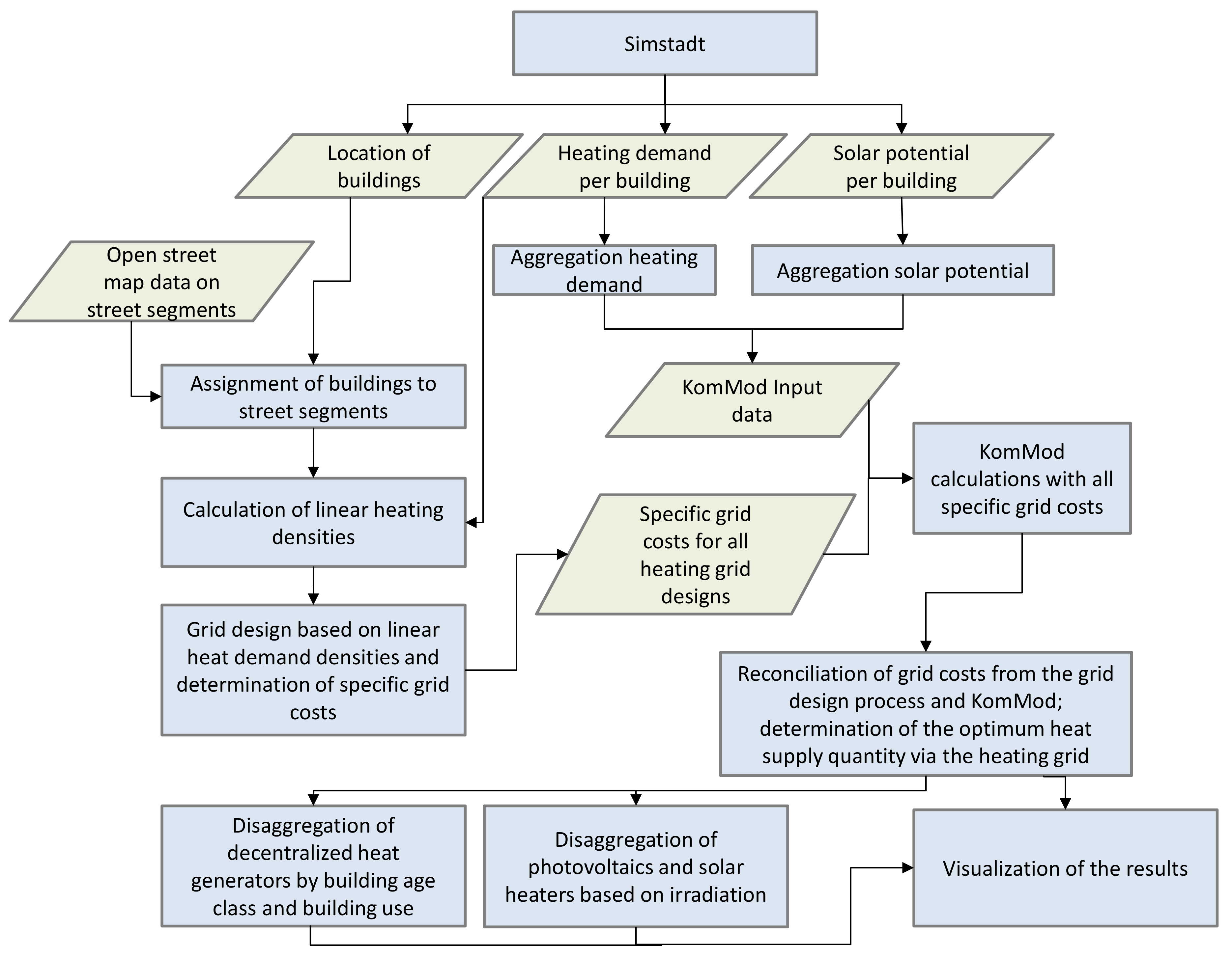
2.2. The Modelling Framework

We introduce SimStadt (Section 2.2.1), KomMod (Section 2.2.2), and a heating grid disaggregation algorithm (Section 2.2.3). Of these, SimStadt calculates building-specific heating demands, KomMod cost-optimal energy systems, and the disaggregation algorithm cost-optimal grid layouts. The challenge in the setup is to determine which part of a city quarter should be supplied by centralized heating in a cost-optimal energy system that provides both electricity and thermal energy. To overcome this challenge, in Section 2.2.4, KomMod and the grid disaggregation algorithm are coupled through two common variables to find both the near-optimal grid layout and annual grid heat supplied. The whole tool chain is shown in Figure 1.

2.2.1. The Simstadt Model

SimStadt is an urban energy system simulation platform under constant development at HFT Stuttgart [36], which currently allows one to assess local energy and water demands (cooling and heating demand [9], electricity profile [37], water demand [38]) and renewable energy potentials (rooftop photovoltaics [9] and bioenergy [39]) on a single-building level or single-field level using 3D city models or digital landscape models in the CityGML format [36]. SimStadt comprises a modular workflow management, with each workflow serving a specific purpose, e.g., heating demand of buildings or photovoltaic potential, while certain modules are shared between workflows.

A 3D building model in CityGML data format serves as basic input for SimStadt. CityGML data files can depict existing environments, such as buildings, roads, and landscape. In this paper, the relevant CityGML object is building objects. Building models are available in five levels of details (LoD), where LoD2 is required to perform a proper energetic analysis, as it includes complete information on the building envelope [9]. Further essential inputs such as building functions, e.g., residential, office, etc., and year of construction [40], can be attached to CityGML files. In the presented cases, the building model for Stöckach is provided by the City Surveying Office, Stuttgart [41], while Baden-Württemberg’s State Office for Geoinformation and Land Development provided the building model for Rainau [42].

In this paper, the per-building heating and domestic hot water demand, and PV potentials on roofs are the basic information. SimStadt calculates the heating demand of each building in a city quarter or larger area as a monthly energy balance according to the German standard DIN 18599 [9]. The general concept of the monthly energy balance is to identify the heat sinks and heat sources in a building zone. Heat sinks describe the heat losses of a zone (e.g., transmission, ventilation, internal, and solar heat losses), whereas heat sources are heat gains (e.g., trough transmission, solar radiation, ventilation, and internal gains). The final heating demand of a building’s zone is then calculated by combining the sum of heat sinks and sources with a degree of utilization.

A building physics library included in SimStadt classifies buildings according to their type and year of construction. For each building type and construction period, information on physical properties of an archetypical building’s wall, roof, and windows are included therein. These properties can then be applied to the actual buildings of a given case study [36]. Similarly, a usage library based on a range of German norms and standards, and focusing on heating set point temperatures, occupancy schedules, ventilation rate and usage-dependent internal gains is consigned. Since outdoor temperatures and solar irradiation are decisive factors for heating demand [43], an integrated weather processor retrieves weather data based on the location of the building model and creates synthetic hourly values for temperature and precipitation from monthly means, if only monthly data is available. If available for a location, climatic data are taken from Meteonorm [44].

The heating period in Germany typically lasts from October to April, while heating demand (excluding domestic hot water demand) is zero over the summer period. To be compatible with the hourly data resolution applied in KomMod, monthly heating demand values are transferred into hourly values according to the German standard VDI 4710 [45]. More detailed information on heating demand simulation can be found in [46,47].

A building’s PV potential can also be assessed with SimStadt based on the same CityGML file and weather data. In the first simulation steps, SimStadt uses the 3D CityGML model to determine the inclination and azimuth for every roof area and calculates the solar irradiance on those surfaces [9]. Different radiation models can be applied, with some taking shading and reflection effects into account [48]. In this study, heating demand and PV potential (considering shading effects) define the basic conditions for subsequent simulation and are run up-front and detached from any subsequent optimization process.

2.2.2. The KomMod Model

KomMod is a linear energy system optimization model that can compute the combined installation and cost-optimal operation of energy supply technologies for the sector’s electricity, heating, cooling and (synthetic) fuels [10]. The model—implemented in AMPL [49] is available in a spatially disaggregated version as well as a version without any explicit spatial disaggregation. As described in Section 1, spatial disaggregation comes with the need for spatially disaggregated data and results in longer computation times, in one case study, for example, the computation time increases from 5 min for the one node model to 6 h for 58 nodes [10]. Consequently, the variant without spatial disaggregation is used for all practical purposes, which allows KomMod’s simplex algorithm (implemented via a gurobi solver [50]) to find the optimal system configuration (if present) in less than ten minutes in most cases. All main energy conversion technologies for supplying electricity, heating, cooling and (synthetic) fuels are implemented in the model: thermal power plants and CHPs, wind power plants, photovoltaics, hydro power plants and fuels cells for electricity supply. For heating supply, we consider heat pumps, solar heaters and boilers, in addition to CHPs and fuel cells. Cooling demand can be met with different kind of chillers. Due to the high temporal resolution, the optimal amount of storage technologies is also assessed with every run for electrical and thermal storages, as is the use of electrolyzers to convert excess electricity to hydrogen and store it for later use.

As input data, technical specifications as well as cost parameters are needed for all technologies. This way, each technology’s lifetime, efficiency, as well as capital and maintenance costs are considered. All cost data are expressed as annuities for the respective technology lifetime. In addition, the potentials for the deployment of different technologies have to be given as a boundary condition, such as rooftop potentials for PV and solar heaters, as well as usable amounts of different fuel types. The energy output of wind energy converters, photovoltaics and solar heaters and the efficiency of heat pumps is calculated based on weather data (e.g., from [44]). Therefore, wind speed, solar irradiation and temperature of the air and the ground have to be fed into the model in the same time resolution as the demand profiles. Temporal demand profiles (given mostly in an hourly resolution) for all relevant demand sectors need to be included. In all scenarios considered here, these are electricity and heat. On top of this, cooling, fuel demands and energy demand for transport can also be considered. Further boundary conditions can be set, e.g., certain thresholds for carbon dioxide emissions, mandatory usage of renewable energy technologies or upper limits for capacities for some technologies.

If Simstadt output is used as input data in KomMod, the building-specific energy demand has to be aggregated to a single hourly-resolved time series when using KomMod’s one-node mode. Solar energy rooftop potentials have to be aggregated to several angles and tilt classes.

One of the key outputs of KomMod used in the proposed modelling framework is the annual amount of heating energy supplied by the combination of all considered heating technologies in a cost-optimal energy system. As KomMod is used as a one-node model, the optimal share of centrally supplied heat cannot be a result of the model itself and makes coupling with the proposed algorithm necessary.

2.2.3. The Heating Grid Disaggregation Algorithm

To extend the definition of a cost-optimal energy system to the heating grid, it is desirable for the heating grid assigned to such energy system to have maximum heating density. In the following, we therefore describe a disaggregation algorithm that generates heating grids based on a 3D building model and the buildings’ associated heating demands. From the wide range of grids generated by the algorithm, a process introduced in Section 2.2.4 chooses the one that is consistent with a cost-optimal energy system as computed by KomMod. The applied consistency condition builds on heating grid costs and the pricing model that assigns a specific cost x to each grid is introduced further below. The basic building blocks of the disaggregation algorithm are street segments, which is that part of a street that lies between two intersections. The 3D building model that is processed in SimStadt to determine heating demand and solar potential also allows us to assign every building in the study area to its nearest street segment. It is then assumed that all buildings assigned to a specific street segment will be connected to the heating grid if this street segment is part of the grid. In reality, grid layouts can differ from this coarse-grained pattern, but such deviations cannot easily be included in an automated algorithm as proposed in this paper.

To choose a heating grid’s first street segment, three approaches are plausible:

• The street segment with the global highest heating density (taken in this paper).
• A street segment adjacent to a potential site for a future heating station.
• The street segment with the highest heating density among all segments adjacent to an existing grid.

The goal is then to generate a sequence of cost-optimal heating grids (of increasing length) by maximizing the respective heating density. To that end, a greedy grid disaggregation procedure is presented that sequentially adds neighboring building clusters of highest heating density to the growing grid. It should be noted that the resulting connected grid—while being composed of segments with locally highest heating density—is not necessarily guaranteed to have itself highest heating density (see Section 4).

Two inputs are required by the disaggregation algorithm: a city street segment model and a so-called look-ahead number. The street segment model includes information on the segments’ heating demands and their lengths, as well as their neighboring segments. The look-ahead number tells the algorithm how “far” to look when assessing the next best segment for the grid’s extension, with look-ahead = 1 meaning that only neighboring segments are considered, while look-ahead = 2 also takes the neighbor’s neighbors into account, etc. After determining the starting point for a heating grid (see above), the algorithm calculates the next best street segment to add to the grid. This is done by searching for the segment or group of segments (look-ahead dependent) with the highest score, with the score defined as the highest coefficient of the sum of all segments’ heating demand divided by the sum of all their lengths. After the sequence of segments with the highest score is determined, only the respective neighbor segment will be added to the grid, because our algorithm is exploratory instead of fully committing. The algorithm continues until all street segments are included. In case the heating grid cannot grow further, implying that all neighbor segments are already part of the grid and there is no street segment connecting the grid to other parts of the city, the first heating grid will be kept as is, and the algorithm starts building a second grid in the same manner as described before.

The left part of Figure 2 illustrates look-ahead 1 and the right illustrates look-ahead 2. Comparing the results shows that look-ahead 2 can better avoid unnecessary dead-end street segments (the lower left part of look-ahead 1 figure) and tends to expand to the more demand-dense area as a cluster (right part of the area). The reason behind this is that the city model contains segments without heating demand, which will not be chosen until there are no other available segments with a demand larger than 0 (case look-ahead 1). Clearly, this strategy fails at some stages of grid expansion, but when using a lookahead of 2, any of the street segments, even those without heating demand, and their neighbors are combined and compared. This can improve foresight in the algorithm, so that new segments are added strategically rather than tactically. However, given the nature of the algorithm, we cannot increase the lookahead without having performance loss. Therefore, the heating grid layout under variable look-ahead 2 is taken for further optimization in the next step.

At each stage of grid expansion in the disaggregation algorithm, the supplied annual heating demand ${\mathrm{Q}}_{\mathrm{G}} \left[\frac{\mathrm{kWh}}{\mathrm{a}}\right]$, total grid length L [m] and specific grid costs x [€/kWh] are calculated. The specific grid cost, defined as the annuity costs divided by the annual heat $Q_G$ that is provided by the grid, is calculated according to Equation (1) [51]. Equation (1) considers annual repayments of a heating grid’s investment cost, which depend mainly on material and construction cost, without costs for operating the grid.

$$\mathrm{x}=\frac{\mathrm{A}·\left({\mathrm{C}}_1+{\mathrm{C}}_2·\left[0.0468m·\ln (\frac{{\mathrm{Q}}_{\mathrm{G}}}{\mathrm{L}}·\frac{m·kWh}{278·a}\right)+0.0007m\right])}{\left(\frac{{\mathrm{Q}}_{\mathrm{G}}}{\mathrm{L}}\right)}$$

(1)

Here, $\mathrm{A} \left[1/\mathrm{a}\right]$ is the annuity factor, ${\mathrm{C}}_1 \left[\frac{€}{\mathrm{m}}\right]$ and ${\mathrm{C}}_2\left[\frac{€}{{\mathrm{m}}^2}\right]$ are constants quantifying the scaling of grid costs with length and diameter, the latter of which is defined by the location of the grid, e.g., urban or rural. As the coupling of grid disaggregation and KomMod is mediated through both $Q_G$ and x, it needs to be ensured that specific heating grid costs are in the same cost category as annuities used in KomMod. This has two implications: first, the annuity factor in Equation (1) shall be the same one used in KomMod’s pricing of energy system components, and second, the values of the cost constants in Equation (1) (C₁, C₂) shall be adjusted for inflation (see also Section 3.1).

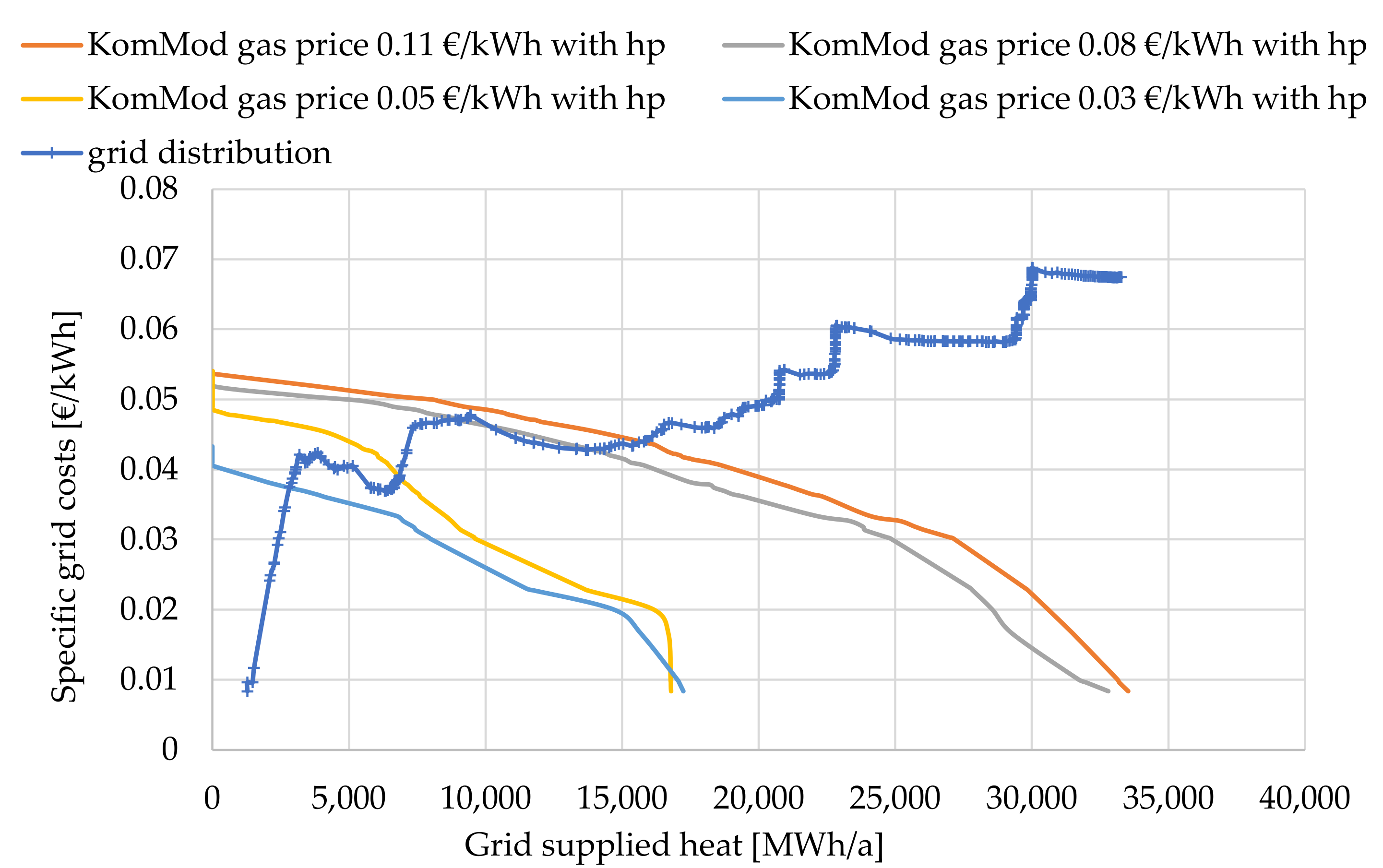
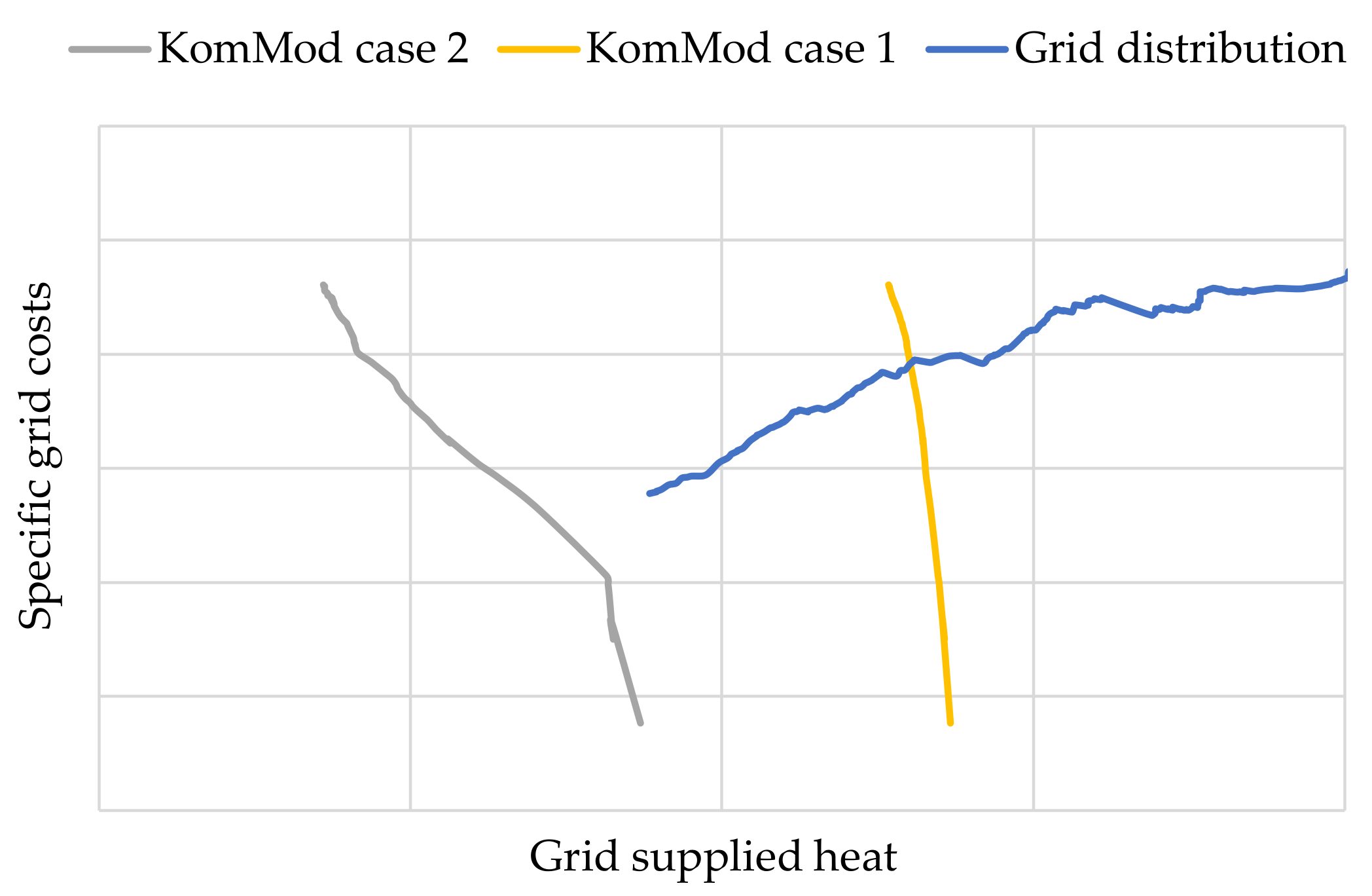
2.2.4. Computing the Optimal Grid

With both the supplied grid heat ${\mathrm{Q}}_{\mathrm{G}}$ and grid length L growing with each step of the grid disaggregation algorithm presented in Section 2.2.3, we want to identify a grid stage that conforms to a cost-optimal energy system as computed by KomMod. This is achieved through linking two variables used both in KomMod and the grid disaggregation algorithm: the specific annual grid cost x and the annual grid heat ${\mathrm{Q}}_{\mathrm{G}}$. The former is an input and the latter an output variable for KomMod, and vice versa for the grid disaggregation algorithm.

While the grid disaggregation algorithm yields multiple pairs (x,${\mathrm{Q}}_{\mathrm{G}}$)—each of which characterize a grid growth stage—similar pairs need to be generated by KomMod. To that end, a heating grid cost surcharge x, masked as fuel costs per kWh, is imposed on all thermal machines capable of central heating. In the subsequent KomMod optimization run, all energy technologies—centralized and decentralized—compete with each other under imposed boundary conditions to determine the most cost-efficient energy system. By adding up the resulting annual heat provided by all technologies with grid surcharge, KomMod yields the annual grid heat ${\mathrm{Q}}_{\mathrm{G}}$ as a function of x.

With both grid disaggregation algorithm and KomMod independently generating two sets of pairs (x,${\mathrm{Q}}_{\mathrm{G}}$), both sets are compared to find a common pair. For this pair, the grid disaggregation algorithm yields a self-consistent heating grid “solution” (in terms of grid layout and annual grid heat supplied) that is part of a cost-optimal energy system. In the case of multiple such grid solutions, the one with lowest grid cost surcharge x is chosen to minimize the overall system cost (e.g., see also Section 3.2.2). Self-consistent solutions are best found graphically through plotting and interpolating both sets of pairs in the x-${\mathrm{Q}}_{\mathrm{G}}$ plane, and subsequently looking for grid solutions closest to the intersection. There, two scenarios are possible:

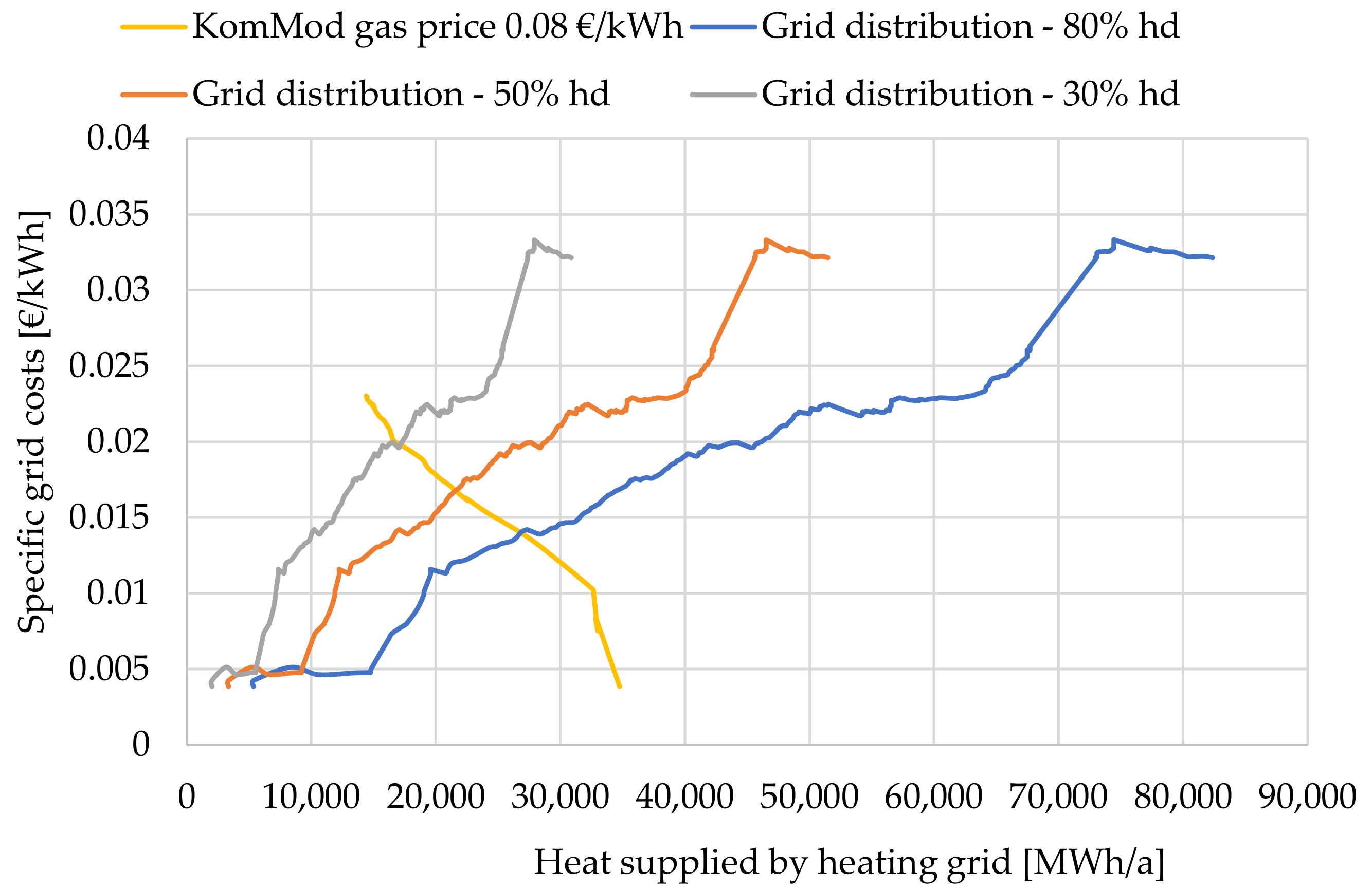
• The two curves have an intersection. In that case, the intersection point yields the optimal amount of grid-supplied heat, as at this point, the specific grid costs from KomMod and the cost determined via the grid distribution algorithm are approximately the same (KomMod case 1 in Figure 3).
• The two curves do not intersect, with the KomMod curve generally yielding smaller values for the grid-supplied heat. In this case, KomMod suggests using district heating only at costs that are lower than the costs associated with heating grid installations in the studied area. Therefore, district heating is economically not feasible. (KomMod case 2 in Figure 3).

It has to be noted that if the heating grid runs through a street segment, all of the segment’s buildings are connected to the grid. Therefore, it is known which buildings in one quarter are supplied with heat via a grid and which buildings have decentralized heating systems. The technologies with a grid surcharge in KomMod are then assigned to the grid, and decentralized technologies without grid surcharge shall be assigned to those buildings located in street segments without grid connection. To that end, the annual heat supplies of different centralized and decentralized heating systems—as given by KomMod—can be used. For assigning decentralized technologies, criteria such as building types and years of construction are taken into account.

3. Results

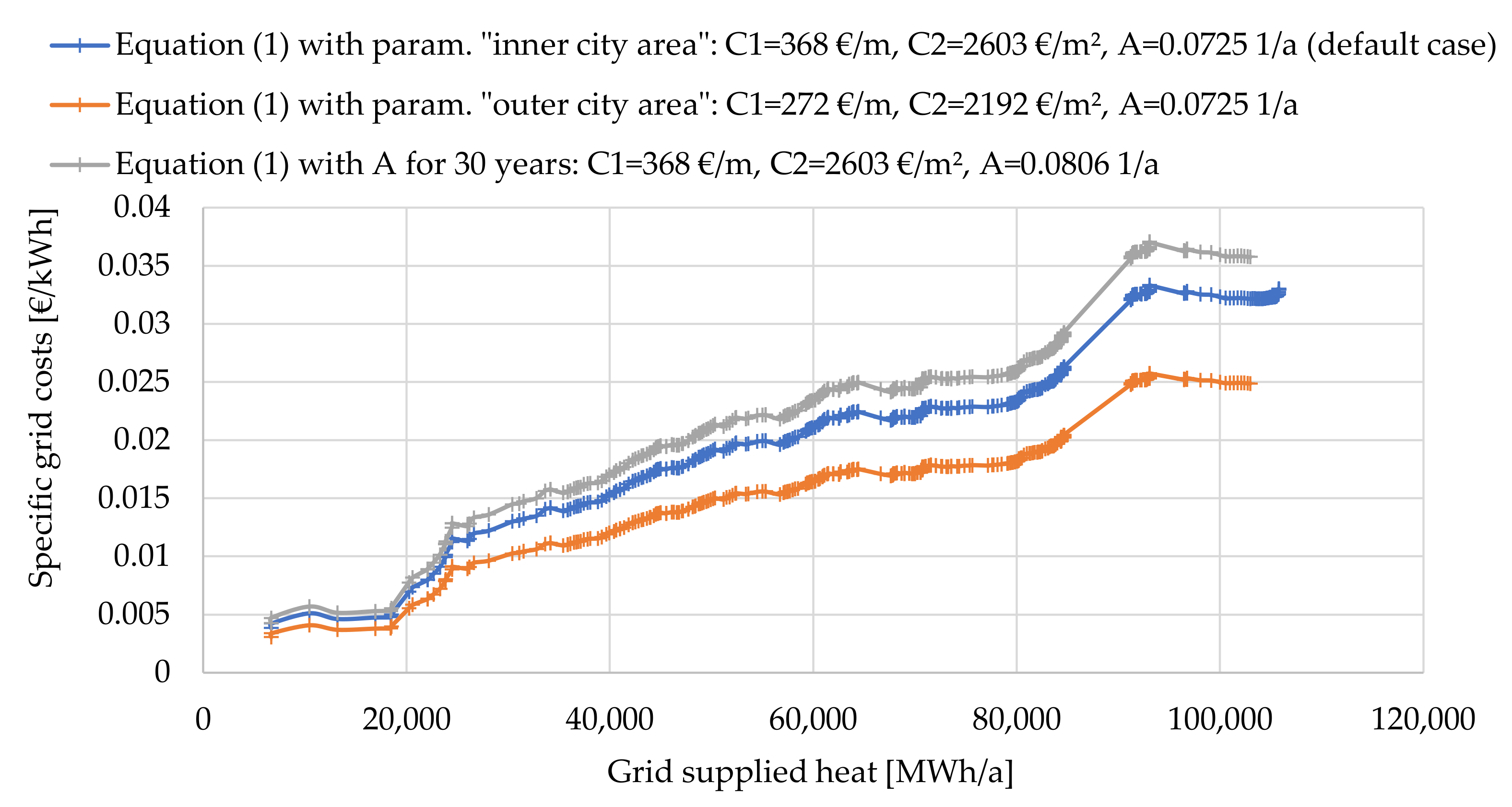
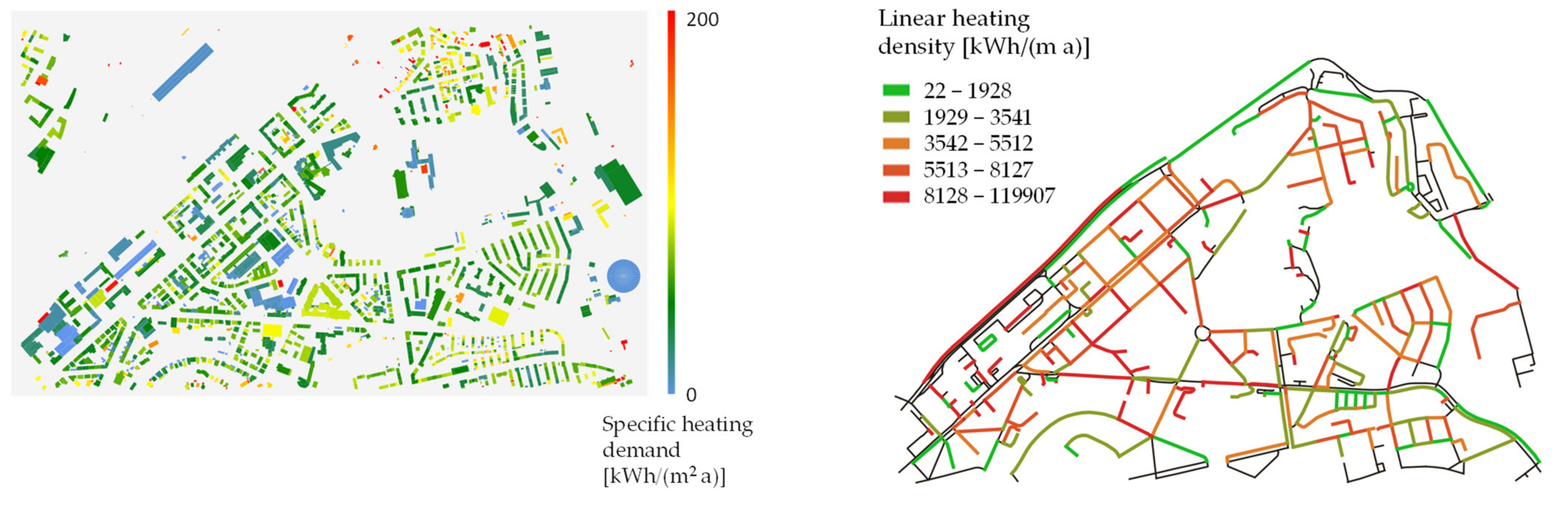
3.1. Linear Heating Density and Grid Costs

Figure 4 shows the specific heating demand for every building and the linear heating density for every street segment based on analysis within SimStadt for the case study area in Stuttgart-Stöckach.

Figure 5 shows the specific grid costs and grid-supplied heat for the case study Stuttgart-Stöckach for different parameters in Equation (1): The blue line gives the default case for an inner-city area, with an annuity factor calculated with 50 years lifetime and an interest rate of 7%. The orange line applies 23% lower construction cost (via parameters ${\mathrm{C}}_1$ and ${\mathrm{C}}_2$ in Equation (1)) than is typically associated with suburban quarters, but might also be achieved if grid building is more coordinated with water or electricity grid maintenance or refurbishments. In contrast, the grey line shows a configuration with 11% higher specific grid costs based on an asset lifetime that is reduced to 30 years. This sensitivity assumes, for example, that heating grids become stranded assets by 2050, as carbon-neutral heating by other means become much more efficient, even in inner-city districts. Taking these results into account, the calculated specific grid costs are assessed as sufficiently robust for our aim.

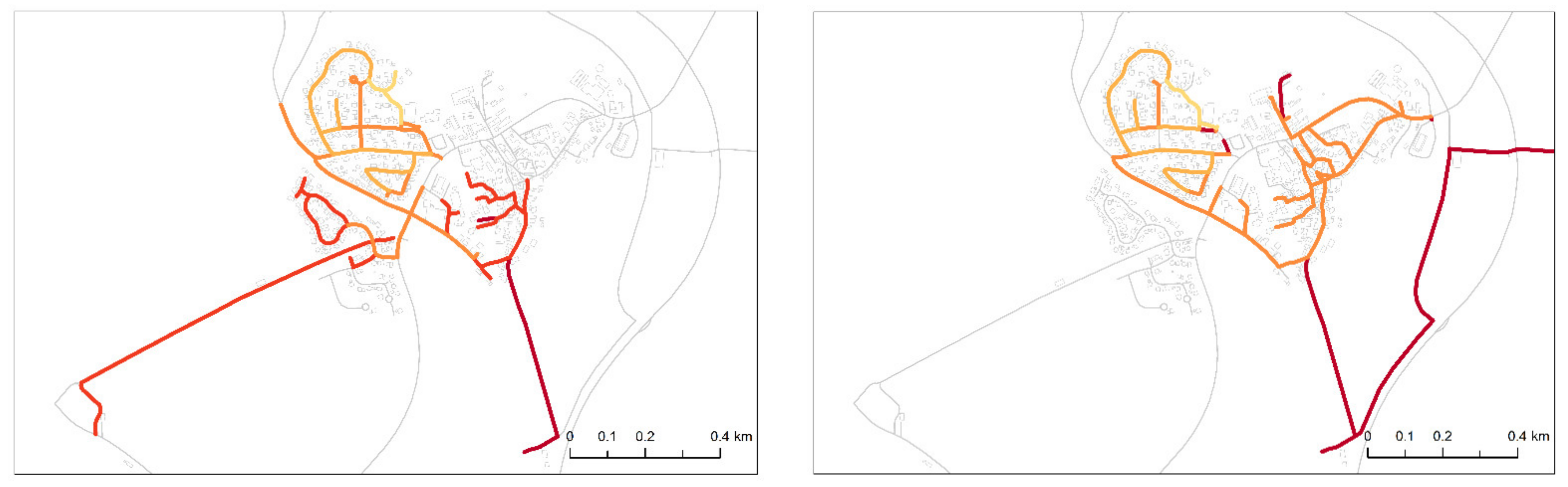
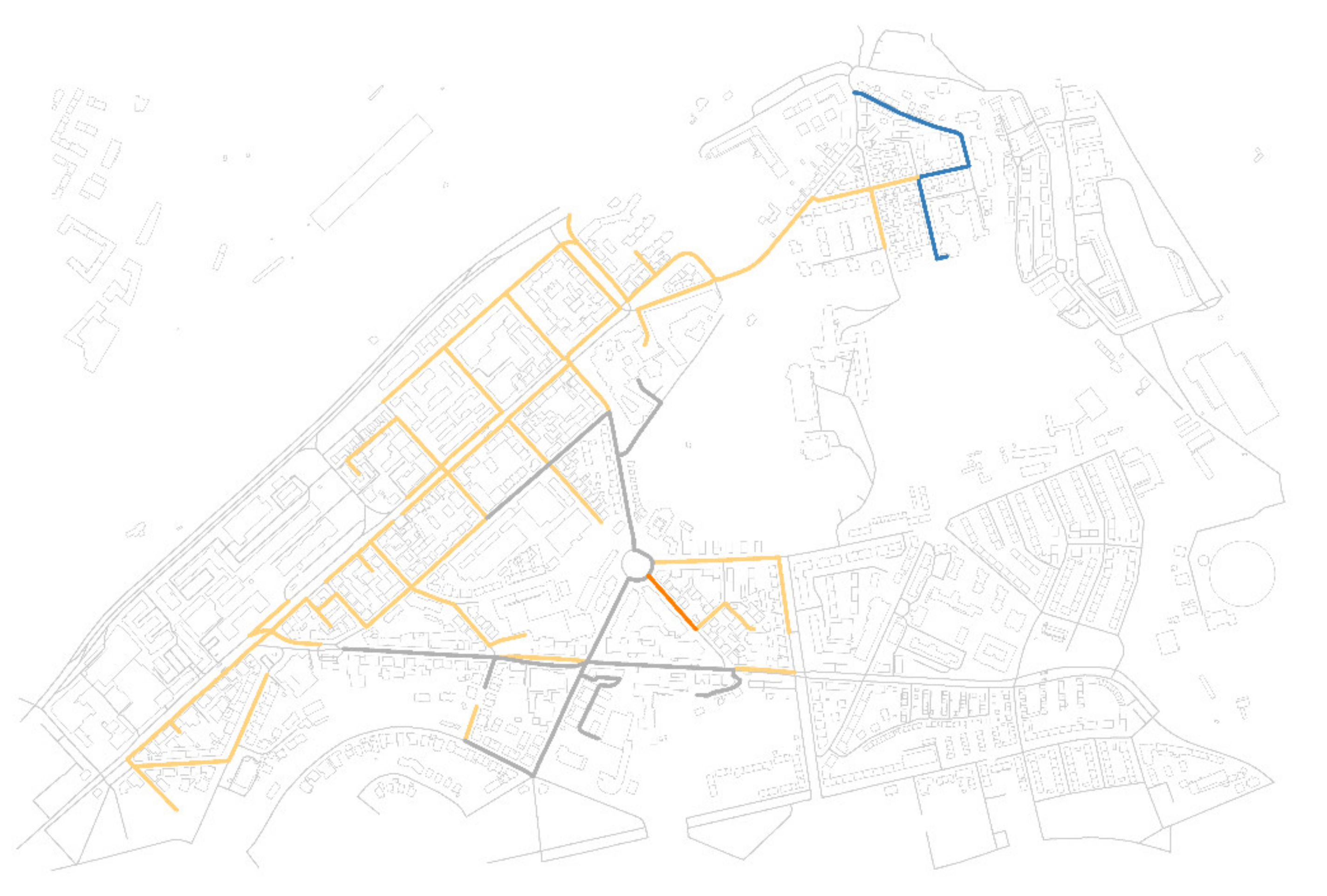
3.2. Optimal Grid Layout

Table 2. Scenario specifications for Stuttgart-Stöckach and Rainau in 2030.

		Stöckach	Rainau
Possible technologies	Electricity converters	Photovoltaic
		Gas-fired CHP
		Import
			Wind power plants
	Decentral thermal converters	Gas and oil boilers	Gas, wood and oil boilers
		Air-sourced heat pumps	Air and ground-sourced heat pumps
		Solar heaters
	Central thermal converters	Gas-fired CHP
		Ground-sourced heat pumps
Cost data	Import electricity price [EUR/kWh]	0.15
	Technology installation and maintenance costs	According to [52]
	Natural gas price [EUR/kWh]	Varied between 0.03 and 0.11
	Price for oil and wood	0.02 EUR/kWh higher than natural gas price (based on historic price differences between gas, oil and wood)

shows the scenario specifications for the two case study areas. Parameters and specifications as similar as possible are chosen to allow for a better comparison of results.

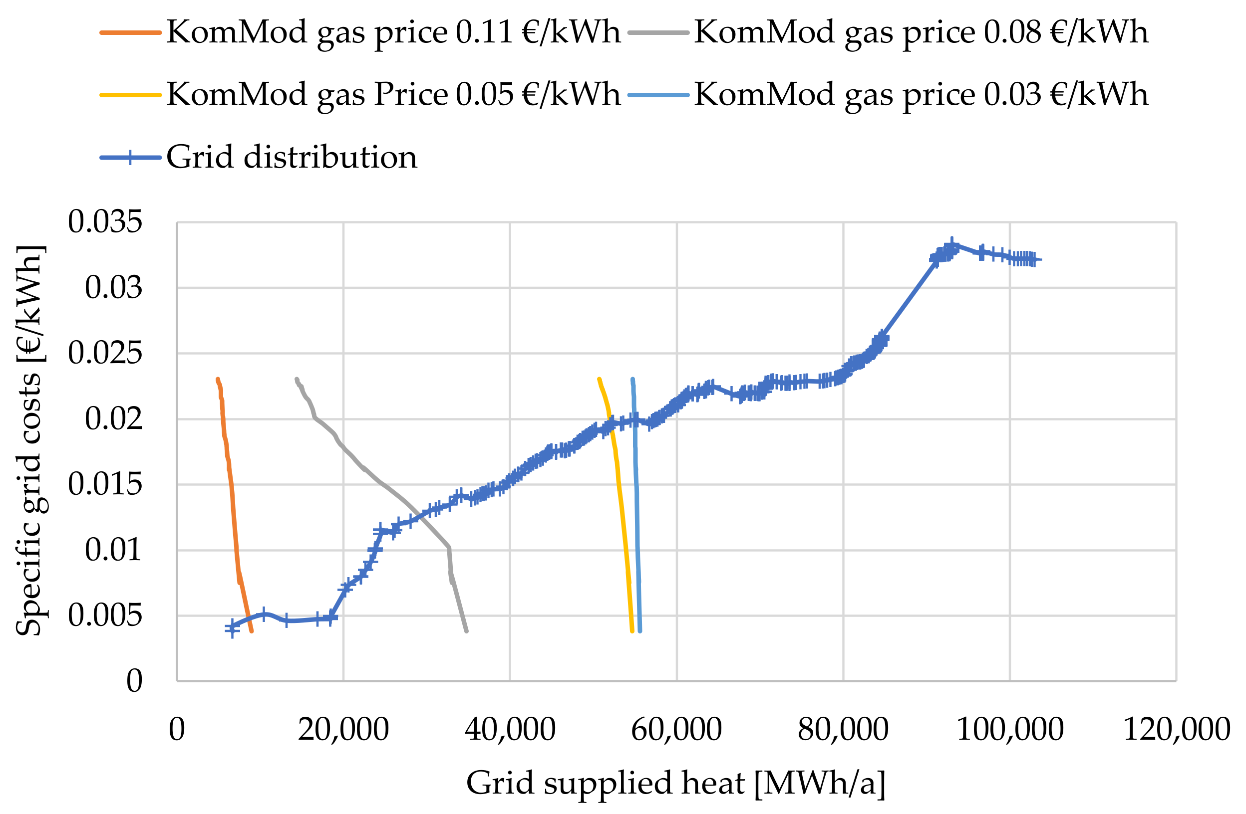
3.2.1. Case Study Stuttgart-Stöckach: Fuel Cost Variation

Figure 6 shows specific grid costs vs. grid-supplied heat for Stuttgart-Stöckach under varying natural gas prices in KomMod, default values for the cost calculation with Equation (1) and lookahead = 2 for the grid distribution algorithm. A gas-fired (centralized) CHP provides heat to the grid. The applied gas price ranges from 0.03 EUR/kWh to 0.11 EUR/kWh, as indicated in Figure 6. As discussed earlier, the respective optimal grid size is indicated by the intersection between the KomMod graphs and the grid distribution curve: as expected, the amount of grid-supplied heat decreases with increasing gas price, as alternative heating options such as heat pumps become relatively more cost-competitive, as the electricity price is kept constant in all four scenarios.

Table 3. Share of centrally supplied heat in the different scenarios in Stöckach and Rainau.

Fuel Price in EUR/kWh	S-Stöckach CHP	S-Stöckach CHP + Heat Pump	Rainau CHP	Rainau CHP + Heat Pump
0.03	51.1%	95.0%	4.5%	8.4%
0.05	49.4%	86.2%		20.3%
0.08	26.5%	91.2%		41.8%
0.11	6.9%	87.6%		47.3%

gives an overview of the share of centrally supplied heat in all scenarios.

A visualization of the four optimal heating grid configurations is given in Figure 7. With a fuel price of EUR 0.11/kWh, only the first grid element is supplied centrally (orange) with heat. With a fuel price of EUR 0.08/kWh, 23 more grid segments with a total length of 6.2 km are connected to the grid (grey), leading to 26.5% of the total heating demand being supplied centrally. When lowering the fuel price to EUR 0.05/kWh, the share of centrally supplied heat nearly doubles to 49.5% and 75 more street segments are connected (yellow).

As linear heating density is lower in that part of the quarter, the total yellow grid length is 15.6 km, which is more than twice as high as the grey and orange part together. With EUR 0.03/kWh as gas price, four more grid segments are added and the heating supply reaches a share of 51.1%.

In a second configuration, a central, ground-sourced heat pump is implemented in the model as a second heating supply technology, in addition to gas CHP. As Stuttgart-Stöckach is densely populated, ground-sourced water/water heat pumps cannot be installed in the majority of buildings, and more inefficient air-sourced heat pumps would have to be used in a decentral setup, whereas a centrally installed larger heat pump might be ground-sourced and therefore have better efficiency. Given the large size of the central heat pump, the effective electricity price charged to the heat supplier is lower than the electricity price that decentral, air sourced, heat pumps in individual buildings would be charged, lowering the centralized heat pump’s levelized costs of heat (LCOH). As a result, at least 88% of the area’s heating demand is covered centrally in the optimal configuration with CHPs and heat pumps have nearly equal shares of supplied heat for EUR 0.03/kWh gas price and rising shares for heat pumps with higher gas prices.

3.2.2. Case Study Rainau: Fuel Cost Variation

For Rainau, the same scenarios are calculated as for Stuttgart-Stöckach. In a CHP-only configuration, a heating grid is economically feasible only if the natural gas price is at EUR 0.03/kWh. In this case, only 4.5% of total heating demand is grid-supplied under given boundary conditions (see Table 3). Given its rural nature, heating densities are lower, and by this, specific grid costs are higher in Rainau than in Stuttgart Stöckach: for example, to supply 25% of the area’s total heating demand, specific grid costs in Stuttgart-Stöckach are EUR 0.012/kWh, but EUR 0.047/kWh in Rainau, i.e., almost four times higher.

The Rainau result nicely illustrates that grid disaggregation curves (here the blue-dotted line in Figure 8) contain the chronology of the whole grid disaggregation. This is because there, moving one data point to the right corresponds to another street segment added in the grid disaggregation algorithm. Hence, a steep rise in the curve indicates the grid running out of heat demand in a neighborhood, and a decrease in the curve points to the grid invading a cluster of street segments with relatively high heating densities. This way, the course of the grid disaggregation can be qualitatively read off that blue-dotted curve.

In contrast to Stuttgart-Stöckach, most buildings in Rainau can, in principle, install ground-sourced heat pumps, as most buildings are single- or two-family houses with gardens. Therefore, and as the results with a CHP-only configuration already indicated, decentral options are more feasible. For the centralized case, it is assumed that the central heat pump benefits from economics and efficiencies of scale, as for example, individual buildings can only install more shallow ground-sourced heat pumps that are less efficient. With the increase of fuel prices, centralized CHPs and local boilers using gas, wood or oil are both less competitive and the centralized ground-sourced heat pump becomes relatively more attractive. Figure 8 shows the results for the combination of gas-fired CHP and ground-sourced heat pumps.

As can be seen, the KomMod curves show a higher elasticity with respect to specific grid cost, which can be attributed to overall higher grid costs because of lower linear heating densities and better decentral heating supply options, namely shallow ground sourced heat pumps, which are economically more favorable when specific grid costs increase. Note also that the KomMod configuration with a gas prize of EUR 0.08/kWh yields three candidates for the energy system’s self-consistent solution to centralized heating. Of these candidates, the one with the lowest specific grid cost was chosen in accordance with Section 2.2.4.

With lower linear heating densities in Rainau than in Stuttgart-Stöckach, the share of centrally supplied heat is lower, ranging from 8.4% to 47.3%. The shares of centrally supplied heat increase with higher fuel prices, as heat pumps are more favorable than boilers in that case.

3.2.3. Case Study Stöckach: Grid Connection

In Germany, there is no obligation to connect to a heating grid in already built-up areas where buildings usually already have a (decentral) heating system installed.

Thus, the share of grid-connected buildings will not achieve 100% in the studied areas. For Stuttgart-Stöckach, a sensitivity analysis was performed, with 80%, 50% and 30% of the heating demand being supplied by the heating grid in the different street segments, at a natural gas price of EUR 0.08/kWh. As Figure 9 shows, the two curves still intersect in all cases, i.e., the heating grid remains economically feasible for (varying) parts of the area. In these cases, the share of centrally supplied heat is decreasing from 26.5% at 100% connectivity rate (see also Table 3) to 25.8%, 20.6%, and 16.1% for connectivity rates of 80%, 50%, and 30%, respectively.

3.3. Summary of the Results

The proposed algorithm has been tested on two case studies to check the robustness and practical applicability for two quite different quarters; one being a densely populated urban city quarter, a typical area for district heating, and the other one being a rural town, an area where normally no district heating would be applied. One of the core parts of the algorithm is the cost calculation for specific grid costs based on Equation (1). Therefore, the robustness of the resulting grid costs based on the input parameters was tested for Stuttgart-Stöckach. Changing the annuity factor substantially by decreasing technology lifetime from 50 to 30 years, as well as taking the constants for outer city area in Equation (1), led to a cost change of 11% higher grid costs for the former and 23% lower grid costs for the latter. As the purpose of the modelling framework is to provide information about possible grid infrastructure in a first planning step, a cost variation of 10–20% is seen as sufficiently robust for our aim. A much higher influence can be seen for the gas price. For Stuttgart-Stöckach, in the scenarios where a gas fired CHP is the only central technology, the amount of centrally supplied heat varies between 7% and 51% depending on the price. Fuel prices are always hard to predict [53] and this leads to uncertainties in the planning process. However, this uncertainty is independent from the planning tool used and one challenge district heating providers are dealing with [54]. A heat pump is therefore installed as a second central supply technology and the share of centrally supplied heat rises to 88–95% showing that the amount of centrally supplied heat is nearly independent from the gas price in that case. When locally installed renewables mainly supply electricity in the future, the electricity price is not dependent on world market prices for fuels, but only on technology costs and local policies, which makes the heat pump a more robust technology choice.

The results for the second case study, the rural town of Rainau, shows that district heating can even be favorable in less densely populated areas. By solely giving the option of a centrally installed CHP only with a gas fuel price of EUR 0.03/kWh, district heating is economically feasible, and only for 4.5% of the total heating demand. However, heat pumps increase the economic feasibility of a heating grid like in Stuttgart Stöckach, in this case, especially when the fuel price is increasing and the levelized costs of heat of decentral boilers is rising. Central heat pumps make use of scale effects in efficiency and use electricity at a lower price. Even with imposed grid costs, they are the better solution than decentral heat pumps and boilers from an economic point of view in the shown scenarios.

4. Conclusions

Here, we present a method to determine the role of central heating in a cost-optimal energy system that can feature multiple (coupled) demand sectors. This is achieved without imposing the length or the overall cost of the respective heating grid. Instead, the coarse-grained grid layout and its annually supplied heat are computed self-consistently through coupling two established tools: a building energy demand simulation model of high spatial resolution and an energy system optimization tool of high temporal resolution. This coupling is provided by a novel heating grid disaggregation algorithm. This makes the presented concept a suitable tool for the planning of district heating grid expansions in city quarters. The major benefit of this approach is that not only is the district heating grid layout planned, but also all sectors are optimized. This is achieved by using an energy system model that has integrated all demand sectors (such as heating and electricity in the presented cases, while in addition, transport and cooling are also possible) and points out technologies to satisfy the respective energy demand for the least possible costs.

One advantage of the proposed framework is that it optimizes (i) overall energy systems; (ii) the respective share of supplied centralized heat; (iii) the layout of the supplying heating grid without minimizing an overarching cost function. Instead, two fast optimization algorithms—one exact for linear point-like energy systems, the other heuristic for heating grid layouts—independently generate two solution curves whose intersection yields features (i)–(iii). The shown methodology is hereby not limited to small building models, but also feasible for a larger area, e.g., the whole city, with a reasonable computation time.

The computational effort involved in the proposed framework stretches to three components —heating demand simulation, energy system optimization, and the heating grid disaggregation algorithm. The computation time of the heating demand simulation by SimStadt is less than 90 s including 3D buildings processing for 1900 buildings in the case study Stöckach. The heating demand simulation is run on a PC with standard performance (Duo-core 2.49 GHz CPU and 8 GB RAM). When increasing the number of buildings, the increase of computation time follows the trend of O(n(log(n)), where n is the number of buildings. The computation time of energy system optimization by KomMod does not change when increasing the numbers of buildings, as KomMod is a one-node energy system optimization tool. In order to find the intersection as shown in Figure 3, several scenarios should be run in KomMod with different specific grid costs. For the case study Stöckach, 50 scenarios are run on a server, with one scenario taking 1:10 min (10 kernels on a server with Intel(R) Xeon(R) CPU E5-2690 v2 @ 3.00 GHz processor and 128 GB ram). If the newly added buildings are located in the existing street segments, the computation time of heating grid disaggregation algorithm does not increase, since heating demand is aggregated at street segment level. If new street segments are created, the computation time will increase following the trend of O(n(log(n)), as new street segment might have one or more neighbours. In general, for the case study Stöckach, the process takes time at the order of magnitude of seconds.

Other existing modelling approaches cannot handle such a high number of individual entities as we could model in our approach (around 500 street segments) and an aggregation is necessary (e.g., [32]). Even with only a few dozen buildings that are modelled as individual entities, the run time of a spatially disaggregated energy system model can easily be a few days to weeks with previous approaches.

The shown methodology should of course be developed further, as there are still some drawbacks. First, no temporal resolution in the grid layout methodology is included, and therefore there is no way to check if the operation of the CHPs during the year corresponds to the heating demand of the connected buildings. However, the full load hours are checked manually. Second, with the current methodology, no sizing of peak load boilers is possible, as a distinction between a decentralized boiler and a central boiler cannot be made. Third, the used grid cost formula could be amended to account for more than just investment costs. Fourth, the grid layout algorithm used here is not guaranteed to yield cost-optimal grids. Instead, it is a search heuristic that—for benign building models—generates heating grids with high heating densities. To strive for connected heating grids with highest heating densities, alternative algorithms such as simulated annealing could be employed.

References

1. Bundesministerium für Wirtschaft und Energie. Zahlen und Fakten: Energiedaten. 2020. Available online: http://www.bmwi.de/DE/Themen/Energie/energiedaten.html (accessed on 28 March 2021).
2. Strogies, M.; Gniffke, P. Berichterstattung unter der Klimarahmenkonvention der Vereinten Nationen und dem Kyoto-Protokoll 2021, Nationaler Inventarbericht zum Deutschen, Treibhausgasinventar 1990–2019, Umweltbundesamt—UNFCCC-Submission; Climate Change; Umweltbundesamt: Dessau, Germany, 2021. [Google Scholar]
3. Lund, H.; Werner, S.; Wiltshire, R.; Svendsen, S.; Thorsen, J.E.; Hvelplund, F.; Mathiesen, B.V. 4th Generation District Heating (4GDH): Integrating smart thermal grids into future sustainable energy systems. Energy 2014, 68, 1–11. [Google Scholar] [CrossRef]
4. Nussbaumer, T.; Thalmann, S. Influence of system design on heat distribution costs in district heating. Energy 2016, 101, 496–505. [Google Scholar] [CrossRef]
5. Dochev, I.; Peters, I.; Seller, H.; Schuchardt, G.K. Analysing district heating potential with linear heat density. A case study from Hamburg. Energy Proc. 2018, 149, 410–419. [Google Scholar] [CrossRef]
6. Nouvel, R.; Zirak, M.; Coors, V.; Eicker, U. The influence of data quality on urban heating demand modeling using 3D city models. Comput. Environ. Urban Syst. 2017, 64, 68–80. [Google Scholar] [CrossRef]
7. Dall’O’, G.; Galante, A.; Torri, M. A methodology for the energy performance classification of residential building stock on an urban scale. Energy Build. 2012, 48, 211–219. [Google Scholar] [CrossRef]
8. Reinhart, C.; Dogan, T.; Jakubiec, J.A.; Rakha, T.; Sang, A. Umi-an urban simulation environment for building energy use, daylighting and walkability. In Proceedings of the 13th Conference of International Building Performance Simulation Association, Chambery, France, 26–28 August 2013. [Google Scholar]
9. Weiler, V.; Stave, J.; Eicker, U. Renewable Energy Generation Scenarios Using 3D Urban Modeling Tools—Methodology for Heat Pump and Co-Generation Systems with Case Study Application. Energies 2019, 12, 403. [Google Scholar] [CrossRef] [Green Version]
10. Eggers, J.-B. Das Kommunale Energiesystemmodell KomMod: Konzeption, Implementierung und Anwendung an den Praxisbeispielen Frankfurt am Main und Freiburg-Haslach; Dissertation; Technische Universität Berlin: Berlin, Germany, 2018. [Google Scholar]
11. Jalil-Vega, F.; Hawkes, A.D. The effect of spatial resolution on outcomes from energy systems modelling of heat decarbonisation. Energy 2018, 155, 339–350. [Google Scholar] [CrossRef]
12. Lopion, P.; Markewitz, P.; Robinius, M.; Stolten, D. A review of current challenges and trends in energy systems modeling. Renew. Sustain. Energy Rev. 2018, 96, 156–166. [Google Scholar] [CrossRef]
13. Prina, M.G.; Casalicchio, V.; Kaldemeyer, C.; Manzolini, G.; Moser, D.; Wanitschke, A.; Sparber, W. Multi-objective investment optimization for energy system models in high temporal and spatial resolution. Appl. Energy 2020, 264, 114728. [Google Scholar] [CrossRef]
14. Yang, J.; Xiang, Y.; Wei, X.; Yao, H.; Liu, J.; Gou, J. Planning-objective based representative day selection for optimal investment decision of distribution networks. Energy Rep. 2020, 6, 543–548. [Google Scholar] [CrossRef]
15. Richter, J. Dimension—A Dispatch and Investment Model for European Electricity Markets. EWI Working Paper 11/03. 2011. Available online: https://www.econstor.eu/handle/10419/74393 (accessed on 20 March 2021).
16. Keirstead, J.; Calderon, C. Capturing spatial effects, technology interactions, and uncertainty in urban energy and carbon models: Retrofitting newcastle as a case-study. Energy Policy 2012, 46, 253–267. [Google Scholar] [CrossRef] [Green Version]
17. Omu, A.; Choudhary, R.; Boies, A. Distributed energy resource system optimisation using mixed integer linear programming. Energy Policy 2013, 61, 249–266. [Google Scholar] [CrossRef]
18. Fazlollahi, S.; Girardin, L.; Maréchal, F. Clustering urban areas for optimizing the design and the operation of district heating energy systems. In Proceedings of the 24th European Symposium on Computer Aided Process Engineering—ESCAPE 24, Budapest, Hungary, 15–18 June 2014. [Google Scholar]
19. Fischer, D.; Härtl, A.; Wille-Haussmann, B. Model for electric load profiles with high time resolution for German households. Energy Build. 2015, 92, 170–179. [Google Scholar] [CrossRef]
20. Kelly, S. Do homes that are more energy efficient consume less energy? A structural equation model of the English residential sector. Energy 2011, 36, 5610–5620. [Google Scholar] [CrossRef]
21. Torabi Moghadam, S.; Delmastro, C.; Corgnati, S.P.; Lombardi, P. Urban energy planning procedure for sustainable development in the built environment: A review of available spatial approaches. J. Clean. Prod. 2017, 165, 811–827. [Google Scholar] [CrossRef]
22. Martinaitis, V.; Zavadskas, E.K.; Motuzienė, V.; Vilutienė, T. Importance of occupancy information when simulating energy demand of energy efficient house: A case study. Energy Build. 2015, 101, 64–75. [Google Scholar] [CrossRef]
23. Wang, D.; Orehounig, K.; Carmeliet, J. Dynamic building energy demand modelling at urban scale for the case of Switzerland. In CLIMA 2016-Proceedings of the 12th REHVA World Congress, Aalborg, Denmark, 22–25 May 2016; Department of Civil Engineering, Aalborg University: Aalborg, Denmark, 2016. [Google Scholar]
24. Hofierka, J.; Suri, M. The solar radiation model for Open source GIS: Implementation and applications. In Proceedings of the Open Source GIS-GRASS Users Conference, Trento, Italy, 11–13 September 2002; pp. 51–70. [Google Scholar]
25. Redweik, P.; Catita, C.; Brito, M. Solar energy potential on roofs and facades in an urban landscape. Sol. Energy 2013, 97, 332–341. [Google Scholar] [CrossRef]
26. Lukač, N.; Žlaus, D.; Seme, S.; Žalik, B.; Štumberger, G. Rating of roofs’ surfaces regarding their solar potential and suitability for PV systems, based on LiDAR data. Appl. Energy 2013, 102, 803–812. [Google Scholar] [CrossRef]
27. Gagliano, A.; Patania, F.; Nocera, F.; Capizzi, A.; Galesi, A. GIS-Based Decision Support for Solar Photovoltaic Planning in Urban Environment. In Sustainability in Energy and Buildings; Springer: Berlin/Heidelberg, Germany, 2013; pp. 865–874. [Google Scholar]
28. Dorer, V.; Allegrini, J.; Orehounig, K.; Moonen, P.; Upadhyay, G.; Kämpf, J.; Carmeliet, J. Modelling the urban microclimate and its impact on the energy demand of buildings and building clusters. Proc. BS 2013, 2013, 3483–3489. [Google Scholar]
29. Kaden, R.; Kolbe, T.H. City-wide total energy demand estimation of buildings using semantic 3D city models and statistical data. In ISPRS Annals of the Photogrammetry, Remote Sensing and Spatial Information Sciences. WG II/2, Proceedings of the ISPRS 8th 3D GeoInfo Conference & WG II/2 Workshop (Volume II-2/W1), Istanbul, Turkey, 27–29 November 2013; Copernicus GmbH: Göttingen, Germany, 2013; pp. 163–171. ISBN 2194-9042. [Google Scholar]
30. Hong, T.; Chen, Y.; Lee, S.H.; Piette, M.A. CityBES: A web-based platform to support city-scale building energy efficiency. Urban Comput. 2016, 14, 2016. [Google Scholar]
31. Mróz, T.M. Planning of community heating systems modernization and development. Appl. Therm. Eng. 2008, 28, 1844–1852. [Google Scholar] [CrossRef]
32. Jalil-Vega, F.; Hawkes, A.D. Spatially resolved model for studying decarbonisation pathways for heat supply and infrastructure trade-offs. Appl. Energy 2018, 210, 1051–1072. [Google Scholar] [CrossRef]
33. Marquant, J.; Omu, A.; Orehounig, K.; Evins, R.; Carmeliet, J. Application of spatial temporal clustering to facilitate energy system modelling. In Proceedings of the BS2015: 14th Conference of International Building Performance Simulation Association, Hyderabad, India, 7–9 December 2015. [Google Scholar]
34. Unternährer, J.; Moret, S.; Joost, S.; Maréchal, F. Spatial clustering for district heating integration in urban energy systems: Application to geothermal energy. Appl. Energy 2017, 190, 749–763. [Google Scholar] [CrossRef] [Green Version]
35. Morvaj, B.; Evins, R.; Carmeliet, J. Optimising urban energy systems: Simultaneous system sizing, operation and district heating network layout. Energy 2016, 116, 619–636. [Google Scholar] [CrossRef]
36. Nouvel, R.; Brassel, K.-H.; Bruse, M.; Duminil, E.; Coors, V.; Eicker, U. SimStadt, a new workflow-driven urban energy simulation platform for CityGML city models. In Proceedings of CISBAT 2015 International Conference “Future Buildings and Districts—Sustainability from Nano to Urban Scale”, Lausanne, Switzerland, 9–11 September 2015; EPFL Solar Energy and Building Physics Laboratory: Lausanne, Switzerland, 2015. [Google Scholar]
37. Köhler, S. Stochastic Generation of Household Electricity Load Profiles in 15-minute Resolution on Building Level for Whole City Quarters. In Proceedings of Energy Challenges for the Next Decade, Ljubljana, Slovenia, 25–28 August 2019; School of Economics and Business, University of Ljubljana: Ljubljana, Slovenia, 2019. [Google Scholar]
38. Bao, K.; Padsala, R.; Thrän, D.; Schröter, B. Urban Water Demand Simulation in Residential and Non-Residential Buildings Based on a CityGML Data Model. ISPRS Int. J. Geo-Inf. 2020, 9, 642. [Google Scholar] [CrossRef]
39. Bao, K.; Padsala, R.; Coors, V.; Thrän, D.; Schröter, B. A Method for Assessing Regional Bioenergy Potentials Based on GIS Data and a Dynamic Yield Simulation Model. Energies 2020, 13, 6488. [Google Scholar] [CrossRef]
40. Zirak, M.; Weiler, V.; Hein, M.; Eicker, U. Urban models enrichment for energy applications: Challenges in energy simulation using different data sources for building age information. Energy 2020, 190, 116292. [Google Scholar] [CrossRef]
41. Landeshauptstadt Stuttgart. Stadtmessungsamt. Available online: https://www.stuttgart.de/vv/verwaltungseinheit/stadtmessungsamt.php (accessed on 11 March 2021).
42. Landesamt für Geoinformation und Landentwicklung, Baden-Württemberg. 3D-Gebäudemodelle. Available online: https://www.lgl-bw.de/unsere-themen/Produkte/Geodaten/3D-Gebaeudemodelle/ (accessed on 2 March 2021).
43. Fischer, D.; Wolf, T.; Scherer, J.; Wille-Haussmann, B. A stochastic bottom-up model for space heating and domestic hot water load profiles for German households. Energy Build. 2016, 124, 120–128. [Google Scholar] [CrossRef]
44. Meteotest. Meteonorm. Available online: https://meteonorm.com/en/ (accessed on 12 August 2020).
45. VDI-Gesellschaft Technische Gebäudeausrüstung. VDI 4710-2: Meteorological Data for Technical Building Sevices Purposes-Degree Days; Verein Deutscher Ingenieure e.V.: Düsseldorf, Germany, 2007. [Google Scholar]
46. Bruse, M.; Nouvel, R.; Wate, P.; Kraut, V.; Coors, V. An Energy-Related CityGML ADE and Its Application for Heating Demand Calculation. Int. J. 3D Inf. Modeling 2015, 4, 59–77. [Google Scholar] [CrossRef]
47. Rossknecht, M.; Airaksinen, E. Concept and Evaluation of Heating Demand Prediction Based on 3D City Models and the CityGML Energy ADE—Case Study Helsinki. ISPRS Int. J. Geo-Inf. 2020, 9, 602. [Google Scholar] [CrossRef]
48. Romero Rodríguez, L.; Duminil, E.; Sánchez Ramos, J.; Eicker, U. Assessment of the photovoltaic potential at urban level based on 3D city models: A case study and new methodological approach. Sol. Energy 2017, 146, 264–275. [Google Scholar] [CrossRef]
49. Fourer, R.; Gay, D.M.; Kernighan, B.W. AMPL: A Mathematical Programing Language. In Algorithms and Model Formulations in Mathematical Programming; Wallace, S.W., Ed.; Springer: Berlin/Heidelberg, Germany, 1989; pp. 150–151. ISBN 978-3-642-83726-5. [Google Scholar]
50. Gurobi Optimization, LLC. Gurobi Optimizer Reference Manual. 2021. Available online: https://www.gurobi.com/wp-content/plugins/hd_documentations/documentation/9.0/refman.pdf (accessed on 11 May 2021).
51. Persson, U.; Werner, S. Heat distribution and the future competitiveness of district heating. Appl. Energy 2011, 88, 568–576. [Google Scholar] [CrossRef]
52. Sterchele, P.; Brandes, J.; Heilig, J.; Wrede, D.; Kost, C.; Schlegl, T.; Bett, A.; Henning, H.-M. Wege zu Einem Klimaneutralem Energiesystem: Die Deutsche Energiewende im Kontext Gesellschaftlicher Verhaltensweisen; Fraunhofer Institute for Solar Energy Systems: Freiburg, Germany, 2020. [Google Scholar]
53. Duic, N.; Stefanic, N.; Lulic, Z.; Krajacic, G.; Puksec, T.; Novosel, T. EU28 Fuel Prices for 2015, 2030 and 2050: Deliverable 6.1: Future Fuel Price Review; Faculty of Mechanical Engineering and Naval Architecture, University of Zagreb: Zagreb, Croatia, 2017. [Google Scholar]
54. Björkqvist, O.; Idefeldt, J.; Larsson, A. Risk assessment of new pricing strategies in the district heating market. Energy Policy 2010, 38, 2171–2178. [Google Scholar] [CrossRef]
Figure 1. Flow Chart and data relations between SimStadt, KomMod and the heating grid distribution algorithm.
Resources 10 00052 g001
Figure 2. Illustration of the search algorithm for the next street segment in the grid distribution algorithm with Rainau as an example. The darkness of the street segments indicates the sequence of grid expansion. The darker the color, the later the street segments are included in the grid (lookahead 1 = left, lookahead 2 = right).
Resources 10 00052 g002
Figure 3. Illustrative relation of specific grid costs to grid supplied heat for the two options of the relative position of the algorithm curve and the KomMod curve.
Resources 10 00052 g003
Figure 4. Specific heating demand for every building in Stuttgart-Stöckach and linear heating density for every street segment.
Resources 10 00052 g004
Figure 5. Specific grid costs over grid-supplied heat with different parameters for Equation (1).
Resources 10 00052 g005
Figure 6. Results for Stuttgart-Stöckach of specific grid costs over grid-supplied heat with CHPs as central heating supplier.
Resources 10 00052 g006
Figure 7. Visualization of the different heating grid configurations for Stuttgart-Stöckach (orange: EUR 0.11/kWh gas price, +grey: EUR 0.08/kWh, +yellow: EUR 0.05/kWh, +blue: EUR 0.03/kWh).
Resources 10 00052 g007
Figure 8. Results for Rainau for specific grid costs over grid supplied heat with CHPs and heat pumps as central heating supplier.
Resources 10 00052 g008
Figure 9. Sensitivity analysis for the share of heating demand that is supplied via the heating grid in Stuttgart-Stöckach (hd = heating demand).
Resources 10 00052 g009