Greenhouse Gas Emission Assessment of Simulated Wastewater Biorefinery

Abstract

A wastewater treatment plant (WWTP) can be considered a system where dirty water enters and fresh water (by means of treatment processes) and other co-products such as sludge and biogas exit. Inside the system, typically, the following steps occur: preliminary treatment, primary treatment, secondary treatment, tertiary treatment, disinfection, and solids handling. The system transforms biomass into several energy and non-energy products, which fall into the definition of a biorefinery. This research compares three simulated WWTP in terms of their environmental greenhouse gas (GHG) emission release to the atmosphere: a generic one (without co-product valorization), one that converts co-products into fertilizer, heat, and electricity, and a third one that converts co-products into heat, electricity, fertilizer, and bioplastic. Heat and electricity are used to provide its energy needs. The chosen impact category is GHG, and the aim is to project the best scenario to the European context in terms of GHG avoidance (savings). The scope is the upstream electricity and natural gas production, the in-use emissions, and the avoided emissions by substituting equivalent fossil-based products. The functional unit is 1 L of sewage (“dirty water”). The GHG savings are evaluated by comparing a generic WWTP scenario, without co-product valorization, with alternative scenarios of co-product valorization. Conventional LCA assuming all the emissions occurs at instant zero is compared to a more realistic environment where for each year, the average of the variable emission pulses occurs. Variable emissions pulses are taken from variable inflows data publicly available from European COST actions (COST Action 682 “Integrated Wastewater Management” as well as within the first IAWQ (later IWA) Task Group on respirometry-based control of the activated sludge process), within the later COST Action 624 on “Optimal Management of Wastewater Systems”). The GHG uncertainty is estimated based on the inputs benchmark data from the WWTP literature and by having different available global warming potential dynamic models. The conventional LCA versus dynamic LCA approach is discussed especially because a WWTP is by nature a dynamic system, having variable inputs along time and therefore variable output GHG emission pulses. It is concluded that heat needs are fully covered by biogas production in the anaerobic digester and combustion, covering its own energy needs and with a potential for heat district supply. Only 30–40% of electricity needs are covered by combined heat and power. Bioplastics and/or fertilizer yields potentially represent less than 3% of current European needs, which suggests the need to reduce their consumption levels. In comparison to generic WWTP, GHG savings are 20%, considering the uncertainty in the benchmark input assumptions. The former is much higher than the uncertainty in the dynamic global warming potential model selection, which means that the model selection is not important in this case study.

1. Introduction

Today, 54% of the world’s population lives in urban areas, a proportion that is expected to increase to 66% by 2050. An urban metabolism can be assumed that is all the activities resulting in the use of food, water, materials, and energy. These activities are responsible for producing heat, greenhouse gas emissions, pollutant emissions, solid waste, and wastewater. Focusing on wastewater, the amount of waste produced on average by 1 population equivalent, 1 p.e., is 200 L/day. This wastewater is rich in nutrients (nitrogen and phosphorous), organics, and microorganisms. According to the European directive 91/271/EEC of 21 May 1991:

• “domestic wastewater” means wastewater from residential settlements and services, which originates predominantly from the human metabolism and from household activities;
• “agglomeration” means an area where the population and/or economic activities are sufficiently concentrated for urban wastewater to be collected and conducted into an urban wastewater treatment plant or to a final discharge point.

Therefore, an agglomeration higher than 2000 p.e. implies that a wastewater treatment plant (WWTP) must “treat” the wastewater by reducing its chemicals, microorganisms, and nutrient loads. The organics load is measured by the chemical oxygen demand, COD, and the biodegradable organic load is measured by the biological oxygen demand, BOD. Nutrient levels must be reduced to levels of 1 mg/L N and 0.01 mg/L P before the effluent be discharged in a water stream. There is a maximum of three treatment processes, the primary treatment, the secondary treatment, and the tertiary treatment.

In the preliminary treatment, solids (e.g., toys, rags) are removed from the influent using filters (with different shapes and sizes) to collect these objects and prevent damage to pumps and other equipment in the remaining treatment stages. In the primary treatment, sedimentation tanks are used to separate sludge from the reaming liquid stream. In the secondary treatment, the organic matter is removed by using biological treatment processes. The sludge is subjected to anaerobic treatment where biogas is flare and dry sludge (after centrifugation) is disposed of in a landfill. The liquid is pumped to another tank where leftover solids and the microorganisms sink to the bottom. Chlorination, ozonation, or ultraviolet (UV) light disinfects the liquid. In the tertiary treatment, the quality of the effluent water is controlled, bearing in mind its destination: irrigation and eutrophication discharge into lakes/reservoirs/estuaries, lowering even further the nutrient (N and P) levels. After the tertiary treatment the WWTP must comply with minimum 70–90% BOD5 25 reduction, 75% COD reduction, and 90% total suspended solids (TSS) reduction.

The aim of the work is to compare several WWTP producing different products for the same 1 L of influent wastewater (different biorefinery) in terms of its GHG emissions (scope upstream electricity, in-use emissions, and avoided fossil-based emissions for substitute products). For the best scenario, an overview is made of the numbers of useful products given back to society that can displace fossil-based ones in the European region (fertilizers, bioplastics, and heat). The time dimension is explored in the analysis by considering constant yearly CO_2eq emissions as opposed to all emissions occurring at time zero. For that, 21 models for the metric global warming potential, including the Bern 2.5D climate model and the Bern 3D, are tested and discussed for the 30-years and 50-years lifetime of the biorefinery.

2. Materials and Methods

In Europe (EU28), piped fresh water for households amounts to 31.8 billion m³/year. The WWTP capacity is 700 p.e. (or 51.100 billion m³/year) [1]. In 2016, plastics consumption amounted to 49.9 Mton [2] and fertilizers demanded 19,719,000 tons [3]. Heat needs amount to 4433 PJ (industry-wide [4]). The European Union (EU) Landfill Directive (1999/31/EC) aims at reducing the amount of landfilled waste. The sludge output from European WWTP has a final fate of landfilling, incineration, and fertilizer. These waste targets aim to drive a transition from a linear to a circular economy.

The scope is to look to a benchmark WWTP with primary, secondary and tertiary treatment, and identify the electricity, heat, N, P, and acid flows. The boundaries exclude construction materials and sewer collecting systems but include upstream impacts of electricity generation and downstream impacts of avoiding fossil-based products. To obtain data for the benchmark, a literature screening is made and summarized in Table 1.

Original sludge fate, landfill, for the generic WWTP is assumed to have a negative GHG impact due to the release of methane emissions [5]. The functional unit is 1 L of influent wastewater or sewage.

2.1. Inventory of WWTP

The methodology is based on the life cycle assessment (LCA) methodology as defined in the ISO 14,040 series.

The scope is to look to a WWTP with primary, secondary, and tertiary treatment and identify the electricity, heat, N, P, and acid flows. The boundaries exclude construction materials and sewer systems, but include upstream impacts of electricity generation, Figure 1. The functional unit is 1 L of influent wastewater or sewage.

The inventory was performed by using literature data for a generic WWTP, trying to obtain a benchmark. The influent wastewater is mainly comprised of water (99.9%) together with relatively small concentrations of suspended and dissolved organic and inorganic solids. After the treatment, the effluent water is considered to be 99% of the influent [6]. The literature data correspond to different geographical coverages, technologies, and time frames. Therefore, for each inventory value, at least three sources were gathered to have a benchmark range. In the reference system, generic WWTP, the sludge is subjected to anaerobic treatment where biogas is flare and dry sludge (after centrifugation) is disposed of in a landfill, the worst case. The latter means a CH₄ release of 0.0167 g CH₄/g_drysludge [7].

Table 1. Inventory for the screened WWTP flows and energy needs per 1 L influent.

Item	Literature #1	Literature #2	Literature #3	Benchmark Average
Electricity pumps Stirring centrifugation, UV disinfection	0.45 Wh [8]	0.59 Wh [9]	5.1 Wh [10]	2.05 Wh
Heat for anaerobic digestion (HAD)	907 J [8]	395 J [11]	790 J [11]	697 J
Calculated natural gas needs (based on HAD and LHV 39 MJ/m3)	2.3 × 10−5 m3	1.0 × 10−5 m3	2.0 × 10−5 m3	1.8 × 10−5 m3
Biogas (60% CH4, 40% CO2) LHV 23.4 MJ/m3	1.1 × 10−4 m3 [11]	2.2 × 10−4 m3 [12]	1.1 × 10−4 m3 [13]	1.5 × 10−4 m3
Biogas electricity by CHP 30% (a)	0.4 Wh	0.2 Wh	0.4 Wh	0.33 Wh
Biogas heat by CHP 70% (a)	1801 J	3604 J	1801 J	2402 J
Biogas (60% CH4, 40% CO2) LHV 23.4 MJ/m3 (d)	8 × 10−5 m3	1.5 × 10−4 m3	8 × 10−4 m3	3.4 × 10−4 m3
Biogas electricity by CHP 30% (a) (d)	0.28 Wh	0.14 Wh	0.28 Wh	0.23 Wh
Biogas heat by CHP 70% (a) (d)	1261 J	2523 J	1261 J	1682 J
Dry sludge	0.43 g (b)	0.39 g [12]	0.79 g [6]	0.54 g
Dry sludge N content	6 mg [8]	20 mg [12]	7 mg [6]	33 mg
Dry sludge P content	9 mg [8]	10 mg [12]	8 mg [6]	9 mg
Primary sludge 30% (c)	0.13 mg	0.12 mg	0.24 mg	0.16 mg
Bioplastic (PHA) (c) (d)	0.03 mg	0.03 mg	0.07 mg	0.04 mg
Avoided Fertilizer (N content + P content)	15 mg	30 mg	15 mg	20 mg

^(a) Electric and heat efficiency from [11]. ^(b) 1720 g/m³ of influent [9], 75% moisture [14]. ^(c) From primary sludge, volatile fatty acids. Primary sludge is typically 30% of total sludge for Europe. PHA 28% cell dry weight [15]. ^(d) W/acids removal.

Table 1. Inventory for the screened WWTP flows and energy needs per 1 L influent.

Item	Literature #1	Literature #2	Literature #3	Benchmark Average
Electricity pumps Stirring centrifugation, UV disinfection	0.45 Wh [8]	0.59 Wh [9]	5.1 Wh [10]	2.05 Wh
Heat for anaerobic digestion (HAD)	907 J [8]	395 J [11]	790 J [11]	697 J
Calculated natural gas needs (based on HAD and LHV 39 MJ/m3)	2.3 × 10−5 m3	1.0 × 10−5 m3	2.0 × 10−5 m3	1.8 × 10−5 m3
Biogas (60% CH4, 40% CO2) LHV 23.4 MJ/m3	1.1 × 10−4 m3 [11]	2.2 × 10−4 m3 [12]	1.1 × 10−4 m3 [13]	1.5 × 10−4 m3
Biogas electricity by CHP 30% (a)	0.4 Wh	0.2 Wh	0.4 Wh	0.33 Wh
Biogas heat by CHP 70% (a)	1801 J	3604 J	1801 J	2402 J
Biogas (60% CH4, 40% CO2) LHV 23.4 MJ/m3 (d)	8 × 10−5 m3	1.5 × 10−4 m3	8 × 10−4 m3	3.4 × 10−4 m3
Biogas electricity by CHP 30% (a) (d)	0.28 Wh	0.14 Wh	0.28 Wh	0.23 Wh
Biogas heat by CHP 70% (a) (d)	1261 J	2523 J	1261 J	1682 J
Dry sludge	0.43 g (b)	0.39 g [12]	0.79 g [6]	0.54 g
Dry sludge N content	6 mg [8]	20 mg [12]	7 mg [6]	33 mg
Dry sludge P content	9 mg [8]	10 mg [12]	8 mg [6]	9 mg
Primary sludge 30% (c)	0.13 mg	0.12 mg	0.24 mg	0.16 mg
Bioplastic (PHA) (c) (d)	0.03 mg	0.03 mg	0.07 mg	0.04 mg
Avoided Fertilizer (N content + P content)	15 mg	30 mg	15 mg	20 mg

^(a) Electric and heat efficiency from [11]. ^(b) 1720 g/m³ of influent [9], 75% moisture [14]. ^(c) From primary sludge, volatile fatty acids. Primary sludge is typically 30% of total sludge for Europe. PHA 28% cell dry weight [15]. ^(d) W/acids removal.

Alternative WWTP #1, Scenario #1, produces biogas that, in a CHP scheme, satisfies the heating needs but avoids only up to 40% of electricity needs. The other product is fertilizer.

Alternative WWTP #2, Scenario #2, produces biogas, fertilizer, and bioplastic from the acids of the primary sludge. The term “bioplastic” means that is considered biodegradable and made from renewable material. The sludge available for biogas is lesser than in SC #1 because part is diverted to bioplastic. Biogas from the secondary sludge, in a CHP scheme, satisfies the heating needs but avoids only up to 30% of electricity needs.

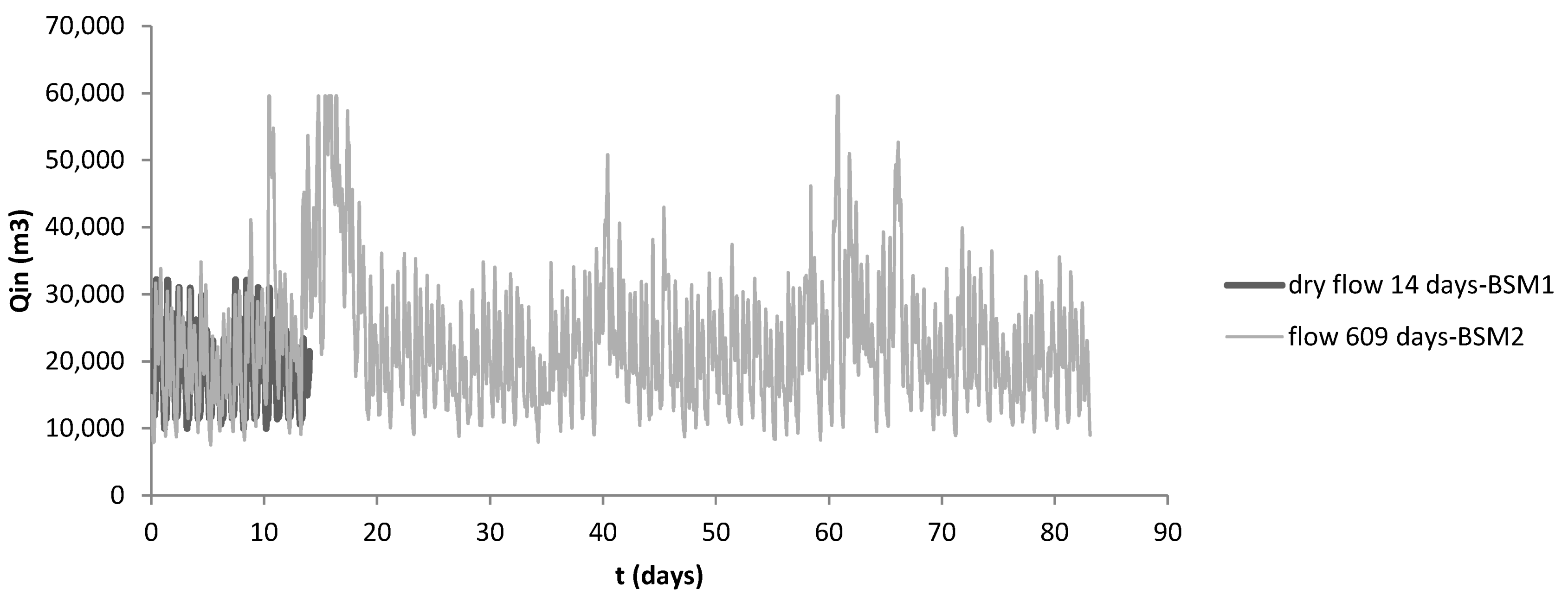
Another issue is considering a dynamic inventory [16] instead of a stationary one. Especially when talking about wastewater, the flow is highly variable throughout a year, and therefore the inventory of consumables and energy needs meets these variable needs. The flow rate and composition of the influent to a WWTP are commonly subject to time variations, i.e., a low rate during the night and high rate during the day, weekend effect, influence of holidays, and seasonal effects.

According to the data gathered from BSM1 and BSM2 datafiles from the IWA Task Group on Benchmarking (COST Action 682 “Integrated Wastewater Management” as well as within the first IAWQ (later IWA) Task Group on respirometry-based control of the activated sludge process), within the later COST Action 624 on “Optimal Management of Wastewater Systems”) [17,18], it was considered that the operation of the plant and the influent it received had variable and cyclic behavior with a period of 1.67 years (609 days, see Figure 2). These open data are very useful to estimate average inflows and outflows per year. In this manner, we can establish an average CO_2eq pulse each year until the 100-year time frame.

2.2. Global Warming Potential

There are several metrics that reflect the climate impact of a technology or supply chain [19]: the global warming potential (GWP), which is the most common, the sustained-flux global warming potential, the instantaneous climate impact, the cumulative climate impact, the technology warming potential, the global temperature change potential, integrated global temperature change potential, the temperature proxy index, the climate change impact potential, the global sea-level rise potential, the integrated global seal level rise potential, the global precipitation change potential, the global damage potential, and the global cost potential.

In this study, the focus is on the metric GWP and on the difference in considering all the emissions occurring at time zero (when the analysis starts, conventional LCA-cLCA) or occurring throughout the biorefinery lifetime (dynamic LCA-dLCA [20]). This framework is depicted in Figure 3, from which we may observe that there are two approaches for the dynamic LCA, which are considering a static inventory or a dynamic inventory. In the first approach to the problem, the static approach is followed.

On top of these LCA possibilities, the uncertainty in the benchmark inputs will have repercussions for the GWP outcomes.

There are several models that allow us to determine the decay of a GHG, CO₂, CH₄, or N₂O in the atmosphere. The instantaneous decaying exponential function’s mathematical expression is [21]:

$${\mathrm{f}}_{\mathrm{CO}2}\left(\mathrm{t}\right)={\mathrm{a}}_0+{\displaystyle \sum }_{\mathrm{n}=1}^3\left({\mathrm{a}}_{\mathrm{n}}{\mathrm{e}}^{-\frac{\mathrm{t}}{{\mathsf{\tau }}_{\mathrm{n}}}}\right)$$

(1)

$${\mathrm{f}}_{\mathrm{CH}4}\left(\mathrm{t}\right)={ \mathrm{e}}^{-\frac{\mathrm{t}}{{\mathsf{\tau }}_{\mathrm{CH}4}}}$$

(2)

$${\mathrm{f}}_{\mathrm{N}2\mathrm{O}}\left(\mathrm{t}\right)={ \mathrm{e}}^{-\frac{\mathrm{t}}{{\mathsf{\tau }}_{\mathrm{N}2\mathrm{O}}}}$$

(3)

The a_n and τ_n vary from model to model, as in

Table 2. Twenty-two models for CO₂ radiative forcing decay [20,21] and GWP_100years for CH₄ and N₂O (1 year time step calculation).

Model	#Years Validity	a0	a1	a2	a3	τ1	τ2	τ3	GWP100 CH4	GWP100 N2O
NCAR	289	2.935 × 10−7	0.3665	0.3542	0.2793	1691	28.36	5.316	17.4	283.3
CSM1.4 HadGEM2-ES	101	0.434	0.1973	0.1889	0.1789	23.07	23.07	3.922	15.4	251.0
MPI-ESM	101	1.252 × 10−7	0.5864	0.231	0.231	178.1	9.039	8.989	16.6	270.6
Bern3D-LPJ (reference)	1000	6.345 × 10−10	0.515	0.2631	0.2219	1955	45.83	3.872	13.2	215.2
Bern3D-LPJ (reference) PI100 w/climate feedback	1000	0.1266	0.2607	0.2909	0.3218	302.8	31.61	4.24	18.1	294.5
Bern3D-LPJ (reference) PI100 w/o climate feedback	1000	0.1332	0.1663	0.3453	0.3551	313.3	29.99	4.601	20.7	338.0
Bern3D-LPJ (reference) PD100 w/climate feedback	1000	6.345 × 10−10	0.515	0.2631	0.2219	1955.5	45.83	3.872	13.2	215.2
Bern3D-LPJ (reference) PD100 w/o climate feedback	1000	0.2123	0.2444	0.336	0.2073	0.2219	1955	45.83	13.0	212.6
Bern3D-LPJ (ensemble)	585	0.2796	0.2382	0.2382	0.244	276.2	38.45	4.928	14.1	230.6
Bern2.5D-LPJ	1000	0.2362	0.09866	0.385	0.2801	232.1	58.5	2.587	16.0	261.3
Bern-SAR	1000	0.1994	0.1762	0.3452	0.2792	333.1	39.69	4.11	16.6	271.0
Bern-378 ppm [20]	1000	0.217	0.259	0.338	0.186	172.9	18.51	1.186	25	298
CLIMBER2-LPJ DCESS	1000	0.2318	0.2756	0.49	0.002576	272.6	6.692	6.692	16.4	267.7
GENIE (ensemble)	1000	0.2145	0.249	0.1924	0.3441	270.1	39.32	4.305	16.1	261.7
LOVECLIM	1000	8.539 × 10−8	0.3606	0.4503	0.1891	1596	21.71	2.281	18.0	294.2
MESMO	1000	0.2848	0.2938	0.2382	0.1831	454.3	25	2.014	13.3	217.6
UVic2.9	1000	0.3186	0.1748	0.1921	0.3145	304.6	26.56	3.8	15.4	250.8
ACC2	985	0.1779	0.1654	0.3796	0.2772	386.2	36.89	3.723	17.5	285.5
MAGICC6(ensemble)	604	0.2051	0.2533	0.3318	0.2098	596.1	21.97	2.995	15.8	256.9
TOTEM2	984	0.000007177	0.2032	0.6995	0.09738	85,770	111.8	0.01583	12.3	199.9
Multimodel mean	1000	0.2173	0.224	0.2824	0.2763	394.4	36.54	4.304	15.6	253.6

. For CH₄, τ_CH4 = 12, and for N₂O, τ_N2O = 114. The 22 model coefficients including the Bern 2.5D climate model for the global warming potential metric and the Bern 3D coefficients are in Table 2.

The GWP is based on the time-integrated radiative forcing due to a pulse emission of a unit mass of gas at nominal time, t = 0. It can be given as an absolute global warming potential for gas x (AGWPx) or as a dimensionless value by dividing the AGWPx by the AGWP of a reference gas, usually CO₂. The GWP, in CO_2eq, is thus defined as:

$$\mathrm{GWPx}\left(\mathrm{t}\right)=\frac{\mathrm{AGWPx}\left(\mathrm{t}\right)}{{\mathrm{AGWPCO}}_2 \left(\mathrm{t}\right)}$$

(4)

and the AGWP for a time t is

$${\mathrm{f}}_{\mathrm{N}2\mathrm{O}}\left(\mathrm{t}\right)={ \mathrm{e}}^{-\frac{\mathrm{t}}{{\mathsf{\tau }}_{\mathrm{N}2\mathrm{O}}}}$$

(5)

where x stands for CO₂, CH₄, and N₂O. When t = TH (time horizon) = 100 years, the values are in Table 2 for 1 year time step calculation. A_x is computed for an atmospheric background CO₂ of 389 ppm [22]: 1.77 × 10⁻¹⁵ W m⁻² kg-CO₂⁻¹; 1.1682 × 10⁻¹³ for CH₄ W m⁻² kg-CH₄⁻¹ (τ_CH4 = 12); and 3.54 × 10⁻¹³ for N₂O W m⁻² kg-N₂O⁻¹ (τ_N2O = 114). A Python in-house program was developed (MultiGLOW.PY) to compute the GWP throughout the years and grasp the difference from the conventional approach, a unique CO_2eq pulse at year 0, to the average emission pulse throughout the facility lifetime, using each of the 22 models, to observe its influence on the outcomes (MultiGLOW.PY In-House python code to assess Multimodel GLObal Warming potential. The in-house python code (version alpha) is available online at https://github.com/carlota200/GHG-dynamic-LCA, accessed on 7 July 2021).

It is noteworthy that the different GWP models cause variations in the methane 100-year GWP (GWP100) between 12.3 and 25.0 and in the N₂O GWP100 between 199.9 and 338.0.

The conventional LCA (cLCA) is obtained by considering all inventory emissions occurring at time zero (first year of operation) and an average wastewater inflow rate, Q_in. The dynamic LCA (dLCA) considers a dynamic wastewater inflow and the pulse emissions occurring throughout the plant lifetime, variable Q_in.

The emission factors for CO₂, CH₄, and N₂O for the several inputs and avoided outputs of the generic and alternative biorefinery are summarized in Table 3. For the electricity indirect emissions, the electricity generation was considered for Europe (EU28) in 2017, according to EUROSTAT, to be 25.6% nuclear, 48.3% thermal, and 26.1% renewables. Considering 200 g/kWh for thermal (natural-gas-based) CO_2eq emissions and 0 g/kWh for nuclear and renewables (emissions only from combustion reactions) gives a GHG emission factor of 97 g/kWh. Of course, this value is variable within the years and could potentially have a range of 0–200 g/kWh, for, respectively, 100% renewables and 100% thermal. CO₂ represents 93%, CH₄ 6%, and N₂O 1% [23].

Natural gas combustion produces 2.75 kgCO₂/kg or, assuming a density of 0.656 kg/m³, 1.8 kgCO₂/m³. Natural gas production and distribution is responsible for 3.08 g/MJ CO₂, 0.19 gCH₄/MJ, and N₂O 0.04 g/MJ [23].

Biogas combustion produces 1.61 kgCO₂/kg or, assuming a density of 1.1 kg/m³, 1.8 kgCO₂/m³ [7]; 10% of the CH₄ is not converted to CO₂, and some N₂O is produced as a function of the Total Kjeldahl Nitrogen (TKN) in the inflow wastewater (0.0050 g N emitted as N₂O/g TKN); considering a typical load of 30–60 mg/L, this would mean 0.15–0.3 mg N₂O/L or 0.150–0.300 kg N₂O per each m³.

Fertilizer production from fossil based sources, 0.57 kgCO_2eq/kg including field application [24], 38% CO₂ (0.22 kgCO₂/kg), 8% CH₄ (0.08 × 0.57/25 = 0.0018 kgCH4/kg), and 38% N₂O (0.38 × 0.57/298 = 0.000727 kgN₂O/kg) only for production.

Plastic production from fossil based sources, 5 kg CO_2eq/kg of PHA [25], 92% CO₂, 7% CH₄ and 1% N₂O [26], i.e., 4.6 kgCO₂/kgPAH, 0.014 kgCH₄/kgPAH, and 0.000168 kgN₂O/kgPAH.

Table 3. Summary of GHG emission factors for the biorefinery inputs and outputs (avoided fossil-based products).

Item/GHG Emission	CO2	CH4	N2O
Electricity production (used or avoided w/biogas CHP) [23]	90.4 g/kWhe	0.021 g/kWhe	0.004 g/kWhe
Natural gas production (used or avoided, w/biogas CHP) [23]	90.9 g/m3	5.6 g/m3	1.2 g/m3
Natural gas burning (used or avoided, w/biogas CHP)	1.62 kg/m3	0.0656 kg/m3	0 kg/m3
Biogas flared [7]	0.0715 kg/m3	1.053 kg/m3	0.225 mg/L inflow
Bioplastics Avoided fossil PHA production [25,26]	−4.6 kg/kgPAH	−0.014 kgCH4/kgPAH	−0.000168 kgN2O/kgPAH
Fertilizers avoided fossil production [24]	−0.22 kg/kgFert	−0.0018 kgCH4/kgFert	−0.000727 kgN2O/kgFert

Table 3. Summary of GHG emission factors for the biorefinery inputs and outputs (avoided fossil-based products).

Item/GHG Emission	CO2	CH4	N2O
Electricity production (used or avoided w/biogas CHP) [23]	90.4 g/kWhe	0.021 g/kWhe	0.004 g/kWhe
Natural gas production (used or avoided, w/biogas CHP) [23]	90.9 g/m3	5.6 g/m3	1.2 g/m3
Natural gas burning (used or avoided, w/biogas CHP)	1.62 kg/m3	0.0656 kg/m3	0 kg/m3
Biogas flared [7]	0.0715 kg/m3	1.053 kg/m3	0.225 mg/L inflow
Bioplastics Avoided fossil PHA production [25,26]	−4.6 kg/kgPAH	−0.014 kgCH4/kgPAH	−0.000168 kgN2O/kgPAH
Fertilizers avoided fossil production [24]	−0.22 kg/kgFert	−0.0018 kgCH4/kgFert	−0.000727 kgN2O/kgFert

Biogas emissions from CHP are the same as in the reference scenario when the biogas is flared. In conventional LCA, the 4th IPCC assessment report equivalency factors were used (25 for CH₄ and 298 for N₂O) to calculate the CO_2eq indicator.

As can be seen in Figure 4, the static inventory (constant emission pulse each year) is an approximation of the dynamic inventory (variable emission pulses on an hourly basis). To quantify the difference, and because we are in the presence of a highly dynamic system (a wastewater treatment plant), it is interesting, at a first stage, to see the influence of cLCA and dLCA (static inventory) in GWP results.

The characterization of GHG absolute emissions of the alternative scenarios (GHG_abs) is the basis to calculate the absolute GHG emission savings (ΔGHG_abs) and the relative GHG savings (ΔGHG_rel).

$$\mathsf{\Delta }\mathrm{GHGabs}= \mathrm{Reference} \left[\mathrm{GHGabs}\right]-\mathrm{Biorefinery}\left[\mathrm{GHGabs}\right]$$

(6)

$$\mathsf{\Delta }{\mathrm{GHG}}_{\mathrm{rel}}=\frac{\mathrm{Reference} \left[\mathrm{GHGabs}\right]-\mathrm{Biorefinery}\left[\mathrm{GHGabs}\right]}{\mathrm{Reference} \left[\mathrm{GHGabs}\right]}$$

(7)

3. Results

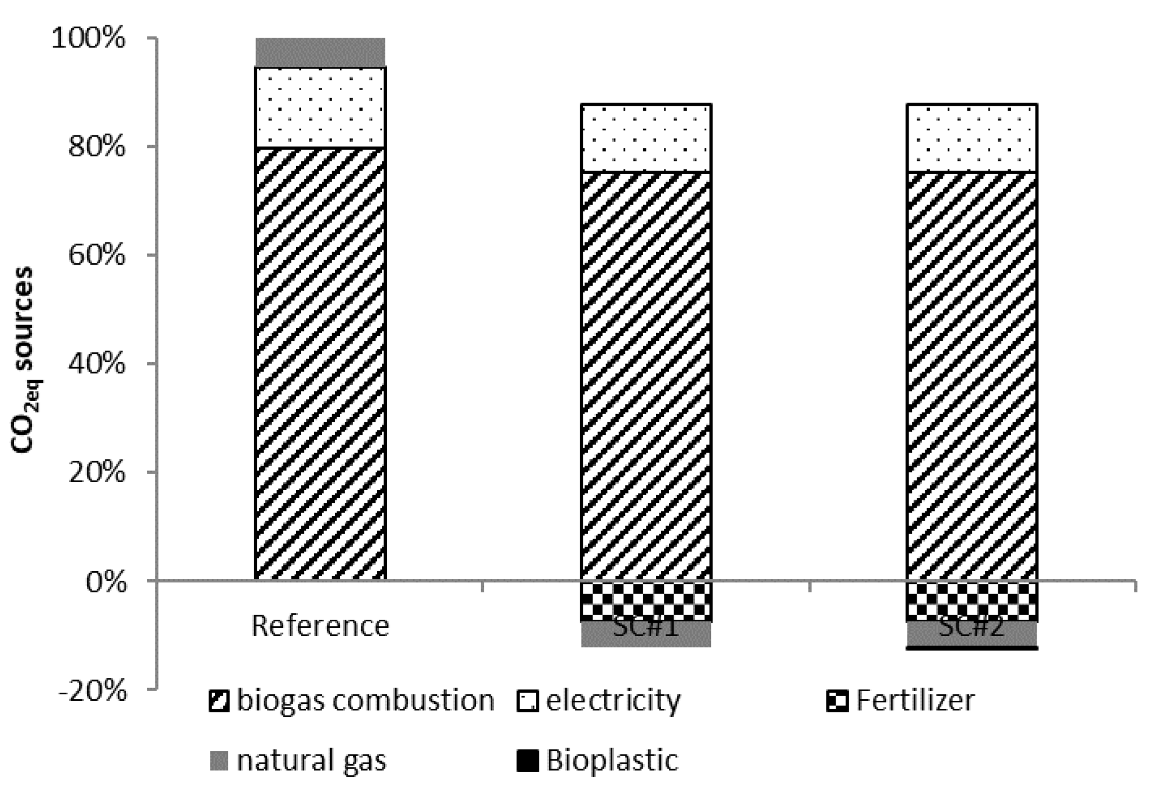
The impact category global warming potential, or GHG emissions, expressed by CO_2eq, was selected to compare the reference WWTP with the other two alternative scenarios. The results, with their respective uncertainty, are depicted in Figure 5. Figure 6 shows the contribution of each item to the overall impact category. Biogas flaring/combustion holds an 80% contribution. The variation in the input quantity per 1 L influent (according to the literature, see Table 1) translates into an uncertainty of up to 146%. Scenario #2 has a similar impact compared with Scenario #1, and both are lower than the reference with the advantage of using their own heat (potentially selling the excess heat to the heating district) and avoiding fossil-based fertilizer. Scenario #2 additionally has the potential to avoid fossil-based plastic, permitting relative GHG savings (ΔGHG_rel) of 20%.

Upstream electricity need was also identified as the item with high uncertainty, which is probably due to the type of disinfection (UV type or chlorine) and more or less pumping. Despite the uncertainty, the best potential scenario, producing bioplastics from the primary sludge volatile fatty acids, is Scenario #2 (SC#2). Roughly 55% of the GHG emissions are from CH₄.

The influence of the time dimension model choice can be seen in Figure 7. The impact of the GHG lifetime decay functions on results could be observed in Figure 7, and variation is within a ±15% range in comparison with the cLCA calculations, depending on the model.

Considering 30 years of operation, and a time horizon of 100 years for the global warming impact, we can see that the difference between conventional and dynamic LCA is 3% at time 100 years but is much bigger at time 20 years (58%). The higher the years of plant operation, the higher these differences, as can be seen in Figure 8 (respectively, 8% and 75% for a 50-year operation). A previous study [27] revealed similar trends with a different case study (biomass to ethanol plant).

Translating these numbers into the European context, we can have an idea of the number of the fossil-based avoided products and of the GHG savings of this future system.

In Europe (EU28), piped fresh water for households amounts to 31.8 billion m³/year. The average WWTP capacity is 700 p.e. (or 51.100 billion L/year) [1]. In 2016, plastics consumption amounted to 49.9 M tons [2] and fertilizer demand to 19,719,000 tons [3].

This could potentially mean that the treated water by biorefinery #3 (Scenario #2) could be converted into 31.5 billion L of fresh water (99% of the needs), 636,000 tons of fertilizer (3% of the needs), and 1378 tons of bioplastics (less than 1% the needs). In terms of GHG savings, ΔGHGabs is 8.2 billion tons and relative GHG savings, ΔGHG_rel, 20%. If a more realistic dLCA is used, savings would be lower, especially if short time frames are considered for the calculations, e.g., 20–30 years.

4. Discussion

The biorefinery concept is typically linked to biomass feedstock transformation into valuable products and came into the discussion in a de-fossilization context [28]. The latter is pressured by climate change and decarbonization [29].

Water consumption for domestic purposes increases due to population growth, which presses for high water quality. If adequate wastewater treatments are implemented and good-quality recycled water is obtained, large areas may be supplied with recycled water that may be used to reduce the water scarcity index. Additionally, wastewater recycling may simultaneously be self-sufficient from an energetic point of view and produce other valuable products for society.

In Europe, the abstraction of fresh water is on average 500 m³/capita, and typically less than 3% of urban wastewater is reused [30]. Water scarcity, referring to long-term water imbalances, combining low water availability with a level of water demand exceeding the supply capacity of the natural system, is seen as an issue in Europe related to climate change and changes in precipitation.

Based on these constraints, wastewater recycling needs, decarbonization, and biorefinery economy nourishing, this study is a first approach that tries to give insight into several water recycling units and their advantages/disadvantages in terms of energy independence, GHG emissions, and the diversion of fossil-based products, fertilizers, bioplastics, and heat.

The novelty here is the consideration of wastewater as a biomass and its transformation into valuable products as a biorefinery. Another novelty is related to the approach followed in accounting for the GHG emissions: consider emission releases concentrated in the first year of operation (conventional LCA approach) or emission releases throughout the operation years (dynamic and more realistic approach). Several models for the dynamic approach were tested to observe the impact on the outcome in relation to the impact of the inputs benchmark range. The study also tackles the most appropriate future biorefinery, providing fresh water and valuable products to society, being self-sufficient from the energy flows point of view.

5. Conclusions

The aim of the work was to compare several wastewater treatment plants (WWTP) producing different products for the same 1 L of influent wastewater in terms of its GHG emissions (scope: upstream electricity emissions, upstream natural gas production, and in-use emissions and downstream emissions avoided from fossil-based equivalent products). For the best scenario useful products for society, besides high-quality water, that can displace fossil-based ones in the European region are made. For a 20-year operation, the overall European amount being 31.8 billion m³/year of sewage, the biogas production is not sufficient to fully satisfy the electric demand of the biorefinery. The electricity needs will be 28.8 TWh/year and the GHG emissions will be 9.8 M ton/year. These future WWTP biorefineries could satisfy 99% of freshwater needs, less than 1% of plastics consumption and less than 3% of fertilizers yearly demands. Despite the low percentages found for the potential contribution of plastic, the strive for consumption patterns may increase the potential replacements’ contribution. For heat, the surplus heat available amounts to a marginal contribution of only 31.3 TJ.

Different GWP models could represent a difference in absolute GHG emission results of up to 15%, which is much less than the uncertainty observed due to inventory benchmark data uncertainty (up to 146%). Therefore, it is more important to assess input benchmark variation than to choose a global warming potential model. The operation lifetime of the plant combined with dLCA is very important to assess a more real absolute GHG emission savings impact throughout the years, especially for short to mid-term assessments 20–30 years rather than for 100-year assessments.

Additional scenarios could be explored in future research, to explore the best option, e.g., bioplastic also using secondary sludge, after the anaerobic digestion, i.e., after biogas production, and microalgae production in the tertiary treatment stage. Microalgae could be a product after harvesting and drying or further processed for bioenergy. Local electricity production by means of solar power could also be exploited once the biogas alone does not provide self-sufficiency of electricity needs.

References

- EurEau. Europe’s Water in Figures An Overview of the European Drinking Water and Waste Water Sectors; EurEau: Brussels, Belgium, 2017. [Google Scholar]
- Europe, Plastics. Plastics the Facts 2014/2015: An Analysis of European Plastics Production, Demand and Waste Data; Plastics Europe: Brussels, Belgium, 2015; pp. 1–34. [Google Scholar]
- FAO. World Fertilizer Trends and Outlook to 2018; FAO: Rome, Italy, 2015; ISBN 9789251086926. [Google Scholar]
- Garcia, N.P.; Vatopoulos, K.; Krook-Riekkola, A.; Rivera, J.A.M.; Lopez, A.P. Heat and Cooling Demand and Market Perspective; Publications Office of the European Union: Luxembourg, 2012. [Google Scholar]
- Piippo, S.; Lauronen, M.; Postila, H. Greenhouse gas emissions from different sewage sludge treatment methods in north. J. Clean. Prod. 2018, 177, 483–492. [Google Scholar] [CrossRef] [Green Version]
- Dong, B. Life-Cycle Assessment of Wastewater Treatment Plants; Massachusetts Institute of Technology (MIT): Cambridge, MA, USA, 2012. [Google Scholar]
- RTI. Greenhouse Gas Emissions Estimation Methodologies for Biogenic Emissions from Selected Source Categories: Solid Waste Disposal Wastewater Treatment Ethanol Fermentation; RTI: Research Triangle Park, NC, USA, 2010. [Google Scholar]
- Lundin, M.; Bengtsson, M.; Molander, S. Life cycle assessment of wastewater systems: Influence of system boundaries and scale on calculated environmental loads. Environ. Sci. Technol. 2000, 34, 180–186. [Google Scholar] [CrossRef]
- Rodriguez-Garcia, G.; Molinos-Senante, M.; Hospido, A.; Hernández-Sancho, F.; Moreira, M.T.; Feijoo, G. Environmental and economic profile of six typologies of wastewater treatment plants. Water Res. 2011, 45, 5997–6010. [Google Scholar] [CrossRef] [PubMed]
- Greg, M.; Matthew, H.; Fitzsimons, L.; Delaure, Y.; Corcoran, B. Life Cycle Assessment of Waste Water Treatment Plants in Ireland. J. Sustain. Dev. Energy Water Environ. Syst. 2016, 4, 216–233. [Google Scholar]
- Bachmann, N.; la Cour Jansen, J.; Bochmann, G.; Montpart, N. Sustainable Biogas Production in Municipal Wastewater Treatment Plants; IEA Bioenergy: Dublin, Ireland, 2015; p. 20. [Google Scholar]
- Fine, P.; Hadas, E. Options to reduce greenhouse gas emissions during wastewater treatment for agricultural use. Sci. Total Environ. 2012, 416, 289–299. [Google Scholar] [CrossRef] [PubMed]
- Pasqualino, J.C.; Meneses, M.; Abella, M.; Castells, F. LCA as a Decision Support Tool for the Environmental Improvement of the Operation of a Municipal Wastewater Treatment Plant. Environ. Sci. Technol. 2009, 43, 3300–3307. [Google Scholar] [CrossRef] [PubMed]
- Tao, J.; Wu, S.; Sun, L.; Tan, X.; Yu, S.; Zhang, Z. Composition of Waste Sludge from Municipal Wastewater Treatment Plant. Procedia Environ. Sci. 2012, 12, 964–971. [Google Scholar] [CrossRef] [Green Version]
- Pittmann, T.; Steinmetz, H. Polyhydroxyalkanoate Production on Waste Water Treatment Plants: Process Scheme, Operating Conditions and Potential Analysis for German and European Municipal Waste Water Treatment Plants. Bioengineering 2017, 4, 54. [Google Scholar] [CrossRef] [PubMed] [Green Version]
- Collet, P.; Hélias, A.; Lardon, L.; Ras, M.; Goy, R.-A.; Steyer, J.-P. Life-cycle assessment of microalgae culture coupled to biogas production. Bioresour. Technol. 2011, 102, 207–214. [Google Scholar] [CrossRef] [PubMed]
- Gernaey, K.V.; Jeppsson, U.; Vanrolleghem, P.A.; Copp, J.B. Benchmarking of Control Strategies for Wastewater Treatment Plants; IWA Publishing: London, UK, 2015. [Google Scholar]
- Rosen, C.; Jeppsson, U. Aspects on ADM1 Implementation within the BSM2 Framework; Technical Reports; Lund University: Lund, Sweden, 2008. [Google Scholar]
- Balcombe, P.; Speirs, J.F.; Brandon, N.P.; Hawkes, A.D. Methane emissions: Choosing the right climate metric and time horizon. Environ. Sci. Process. Impacts 2018, 20, 1323–1339. [Google Scholar] [CrossRef] [PubMed] [Green Version]
- Levasseur, A.; Lesage, P.; Margni, M.; Deschěnes, L.; Samson, R. Considering time in LCA: Dynamic LCA and its application to global warming impact assessments. Environ. Sci. Technol. 2010, 44, 3169–3174. [Google Scholar] [CrossRef] [PubMed]
- Forster, P.; Ramaswamy, V.; Artaxo, P.; Berntsen, T.; Betts, R.; Fahey, D.W.; Haywood, J.; Lean, J.; Lowe, D.C.; Myhre, G.; et al. Changes in Atmospheric Constituents and in Radiative Forcing Chapter 2; Cambridge University Press: Cambridge, UK, 2007. [Google Scholar]
- Joos, F.; Roth, R.; Fuglestvedt, J.S.; Peters, G.P.; Enting, I.G.; Von Bloh, W.; Brovkin, V.; Burke, E.J.; Eby, M.; Edwards, N.R.; et al. Carbon dioxide and climate impulse response functions for the computation of greenhouse gas metrics: A multi-model analysis. Atmos. Chem. Phys. 2013, 13, 2793–2825. [Google Scholar] [CrossRef] [Green Version]
- Edwards, R.; Larive, J.-F.; Rickeard, D.; Weindorf, W. Well-to-Wheels Analysis of Future Automotive Fuels and Powertrains in the European Context WELL-TO-TANK (WTT) Report. Version 4.; Publications Office of the European Union: Luxembourg, 2013; ISBN 9789279338885. [Google Scholar]
- Hasler, K.; Bröring, S.; Omta, S.W.F.; Olfs, H.W. Life cycle assessment (LCA) of different fertilizer product types. Eur. J. Agron. 2015, 69, 41–51. [Google Scholar] [CrossRef]
- Narodoslawsky, M. LCA of PHA Production—Identifying the Ecological Potential of Bio-plastic. Chem. Biochem. Eng. Q. 2015, 29, 299–305. [Google Scholar] [CrossRef]
- Patel, M.; Bastioli, C.; Marini, L.; Würd, D.E. Biopolymers Online—Environmental Assessment of Bio-Based Polymers and Natural Fibres; Utrecht University: Utrecht, The Netherlands, 2005. [Google Scholar]
- Pacheco, R.; Silva, C. Global Warming Potential of Biomass-to-Ethanol: Review and Sensitivity Analysis through a Case Study. Energies 2019, 12, 2535. [Google Scholar] [CrossRef] [Green Version]
- Lindorfer, J.; Lettner, M.; Hesser, F.; Fazeni, K.; Rosenfeld, D.; Annevelink, B.; Mandl, M. Technical, Economic and Environmental Assessment of Biorefinery Concepts. 2019. Available online: https://www.ieabioenergy.com/wp-content/uploads/2019/07/TEE_assessment_report_final_20190704-1.pdf (accessed on 27 July 2021).
- JRC. Deployment Scenarios for Low Carbon Energy Technologies; JRC: Ispra, Italy, 2019. [Google Scholar]
- European Comission. Towards Efficient Use of Water Resources in Europe; European Comission: Brussels, Belgium, 2012.
Figure 1.
Biorefinery of a WWTP system: (a) reference—generic WWTP, (b) Scenario #1, and (c) Scenario #2. Boundaries for the WWTP biorefinery system (- - -).
Figure 2.
Variable inflow (Qin) into a WWTP [17,18]. Open data from COST Action 682 “Integrated Wastewater Management”.
Figure 3.
Framework for the cLCA and dLCA.
Figure 4.
Dynamic versus static inventory emission pulses for the first year of biorefinery#3 (Sc #2) operation, based on Qin from Open-data COST Action 682 “Integrated Wastewater Management”.
Figure 5.
CO2eq for each WWTP biorefinery, cLCA, using 4th AR IPCC equivalency factors.
Figure 6.
Contribution of each item to CO2eq, conventional LCA, 4th AR IPCC.
Figure 7.
Variation in CO2eq for 100 years and for the 21 models (Table 2), SC#2 WWTP biorefinery, cLCA as reference (0%). Case study based on Qin from Open-data COST Action 682 “Integrated Wastewater Management”, see Figure 2.
Figure 8.
CO2eq as a function of time (years after first emission pulse) for the Bern-378 ppm model and biorefinery #3 (Scenario #2), stationary inventory, cLCA vs. dLCA, 30 and 50 years of operation. Case study based on Qin from Open-data COST Action 682 “Integrated Wastewater Management”.