
Opportunities and Challenges of the European Green Deal for the Chemical Industry: An Approach Measuring Innovations in Bioeconomy


Abstract
:1. Introduction
2. Materials and Methods
2.1. Framework for the Assessment
2.1.1. Evaluation of Relevant Biomass Resources
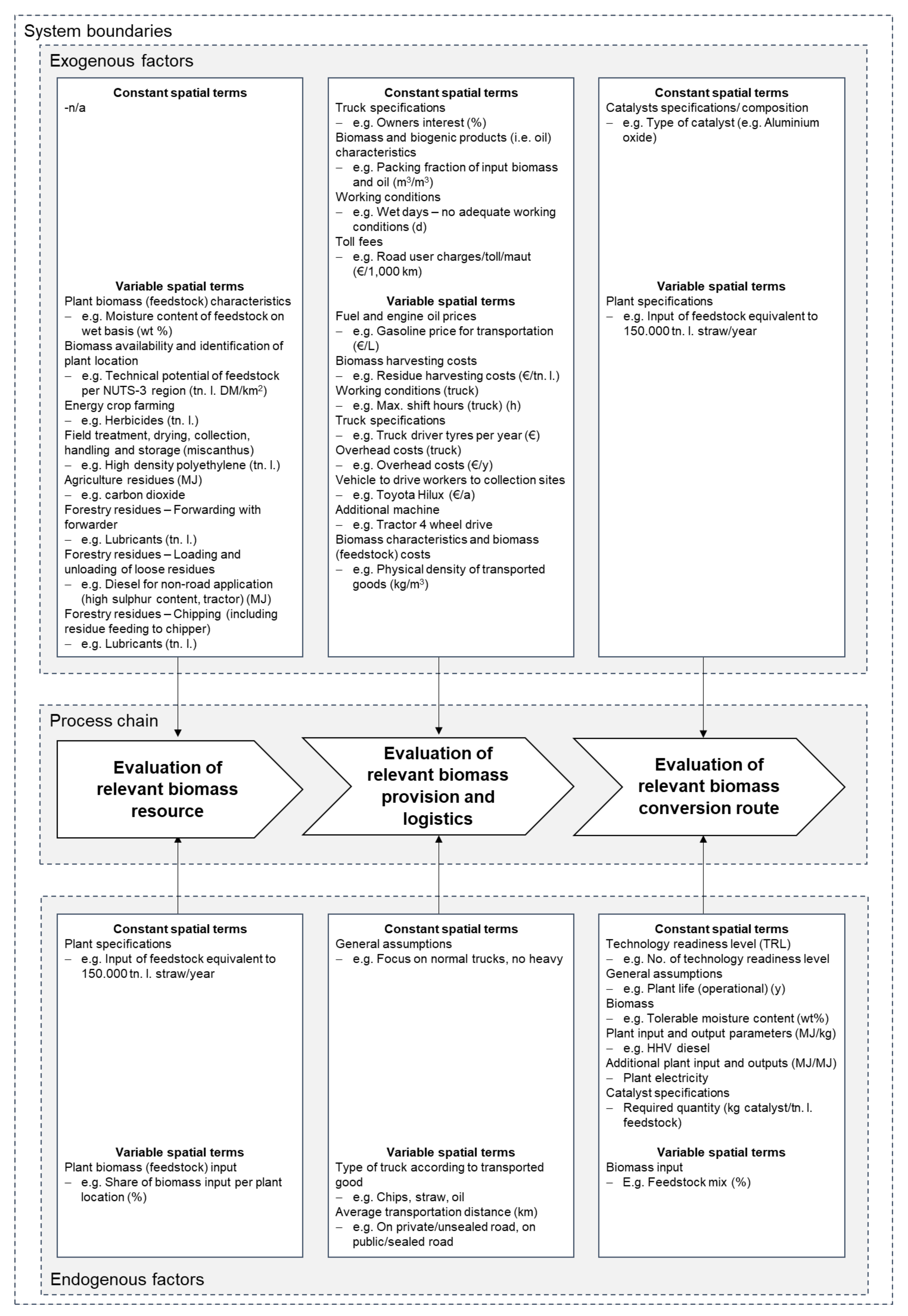
System Definition and Identification of System Boundaries
Data Basis
2.1.2. Evaluation of Relevant Biomass Provision and Logistics
System Definition and Identification of System Boundaries
- (i)
- the chemical raw material properties (e.g., chemical composition, content of biogenic material, amount of trace elements, and water content, as well as chemical stability);
- (ii)
- the physical raw material properties (e.g., quantity, density, ash content, particle size);
- (iii)
- other raw material properties (e.g., origin, yield, seasonal availability, availability against competing uses, harvest time, transportation capacity, ease of transport, suitability for storage, storage stability, long term quality, technical suitability) [15].
Data Basis
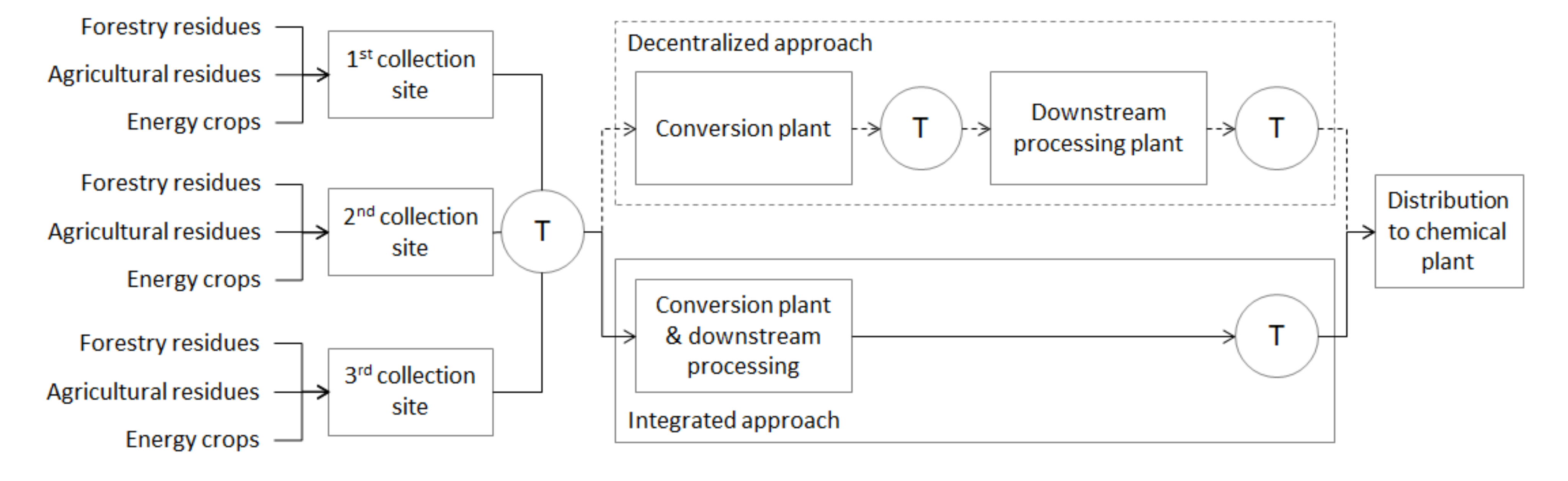
- Feedstock availability is evenly distributed over a circular feed supply area (e.g., NUTS-3 region);
- The conversion plant is located centrally within the respective region (i.e., to minimize the total direct distance from all of the feed sources to the conversion plant);
- Where multiple conversion plants are located in one catchment area (i.e., feed supply area), the location of each conversion plant will be the centroid of the sector that supplies it with the feedstock;
- The road infrastructure and network is ordinary to allow the use of a single winding factor to assess the actual distance from between feedstock source and conversion plant based on the direct distance between source and conversion plant (e.g., radius).
2.1.3. Evaluation of Relevant Biomass Conversion Routes
System Definition and Identification of System Boundaries
Data Basis
2.2. Assessment Methods
2.2.1. Technical Assessment
Key Performance Indicators
Methods for Forecasting
2.2.2. Economic Assessment
Key Performance Indicators
- Capital-related costs (e.g., technical and structural installation, noise protection, and thermal insulation measures and utility connection costs):
- Demand-related costs (e.g., energy costs, costs for operating materials);
- Operation-related costs (e.g., cleaning, servicing, inspection, maintenance);
- Miscellaneous costs (e.g., planning costs, insurance, taxes, administration costs).
- Summary procedures; i.e., to assess the capital costs of a plant, a correlation between specific plant data (e.g., annual turnover) and the plant capacity is calculated by the use of a turnover ratio. This approach shows inaccuracies of about 50%;
- Factor-based methodologies; i.e., include module concepts and global and differentiated surcharge factors. Based on the technical specification of a plant, modules are aggregated and further assessed by factors to estimate the costs of new facilities. A typical multiplier for a new unit within a refinery to estimate the total installed costs of the plant is the Lang factor, describing a ratio of the total installation costs to the costs of the major technical components in a plant. This approach shows inaccuracies of about 30%. An increase in accuracy can be achieved by differentiating global factors according to the state of aggregation of input materials, intermediate products, and final products;
- Individual equipment assessment; i.e., for an individual assessment of all cost parameters, high costs for engineering services are necessary. This approach shows inaccuracies of about 5%.
Methods for Forecasting
2.2.3. Environmental Assessment
Key Performance Indicators
- Classification. The classification assigns emissions to impact categories according to their potential effects;
- Normalization. The expression of the impact potentials are considered in relation to a reference situation (e.g., person-equivalence, PE). The normalized impact potential, nIP, can be defined as displayed in Equation (27) (normalization reference, NR) [44].
- Valuation. The weights are ranked, grouped, or assigned depending on the different impact potentials (weighted impact potential, wIP, weighting factors, WF) (Equation (28)) [44].
Methods for Forecasting
3. Case Study
3.1. System Definition
- Time horizon. The time horizon is the current status (i.e., 2017), the medium term (i.e., 2030), and the long term (i.e., 2045);
- Location. The application examples focus on the EU-28;
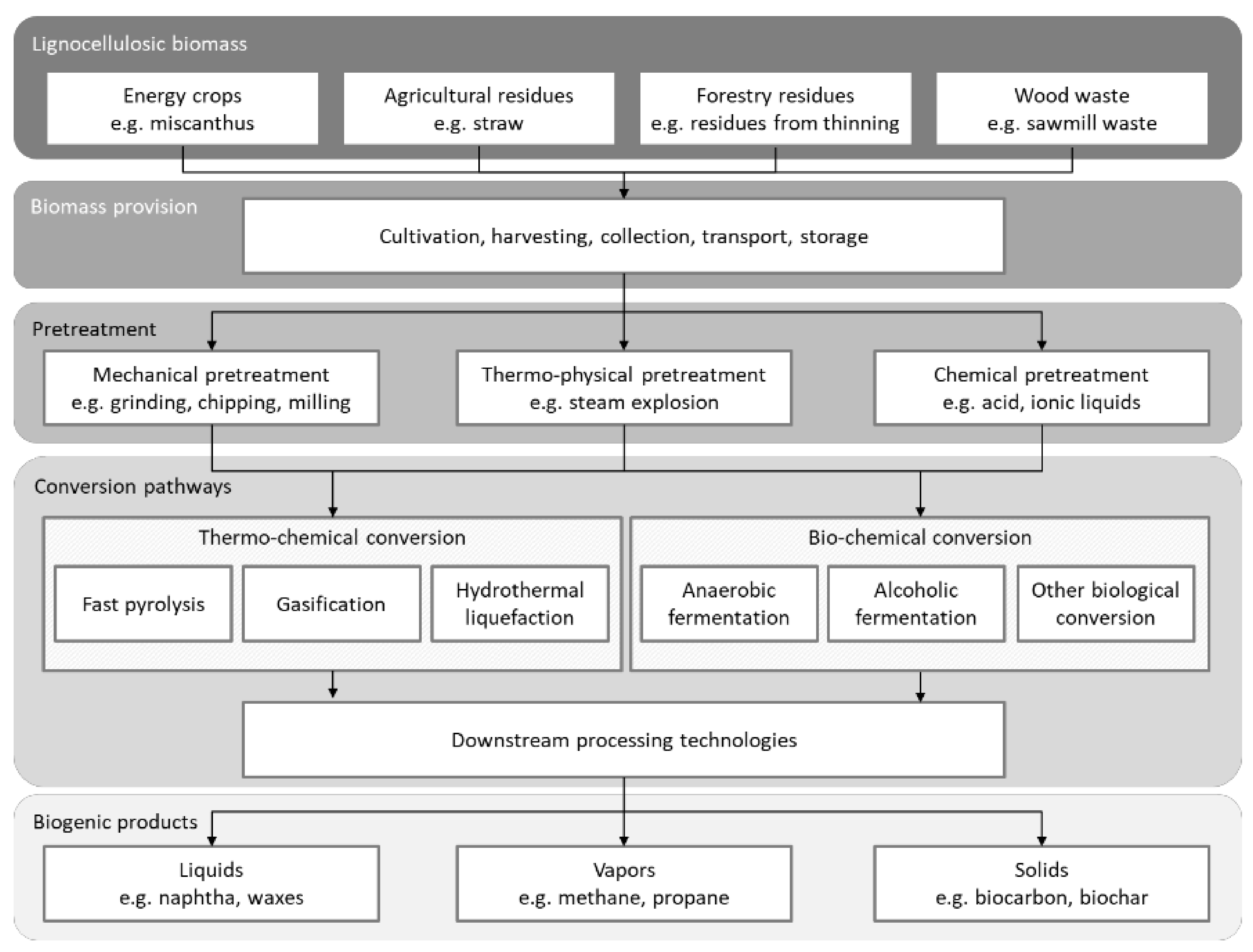
- Lignocellulosic biomass. The only biomass theoretically available as a raw material for the chemical industry is exclusively residual biomass, or biomass cultivated on non-arable or marginal/degraded land. The criterion considered for the selection of the feedstock is the technical potential for different types of lignocellulosic biomass resources in the selected regions: (i) forest residues; (ii) agricultural crop residues; and (iii) energy crops;
- Conversion pathways. The thermo-chemical conversion pathways exemplary evaluated are pyrolysis and gasification;
- Plant capacity. The plant capacity is set to a fixed amount of input biomass to the plant to ensure comparability;
- Plant locations. The countries where the plants are located are in northern Europe, Sweden, in central Europe, Germany, and in southern Europe, Spain.
3.1.1. Determination of Relevant Biomass Resources
3.1.2. Determination of Relevant Biomass Provision and Logistics
3.1.3. Determination of Relevant Biomass Conversion Routes
3.2. Data Basis
3.2.1. Technical Assessment
3.2.2. Economic Assessment
- For the total (installed) equipment costs, no differentiation was considered between the three regions (i.e., Northern Europe, Central Europe and Southern Europe);
- The assessment neither considers any policy factors (e.g., carbon credits, subsidies, mandates, nor tax for the final transportation fuel product);
- The interest rate is set to 4% [62];
- The economic plant lifetime is 20 years according to the technical plant lifetime;
- The biomass input is set to 150,000 tDM/a.
3.2.3. Environmental Assessment
3.3. Results
3.3.1. Technical Assessment
Current Status
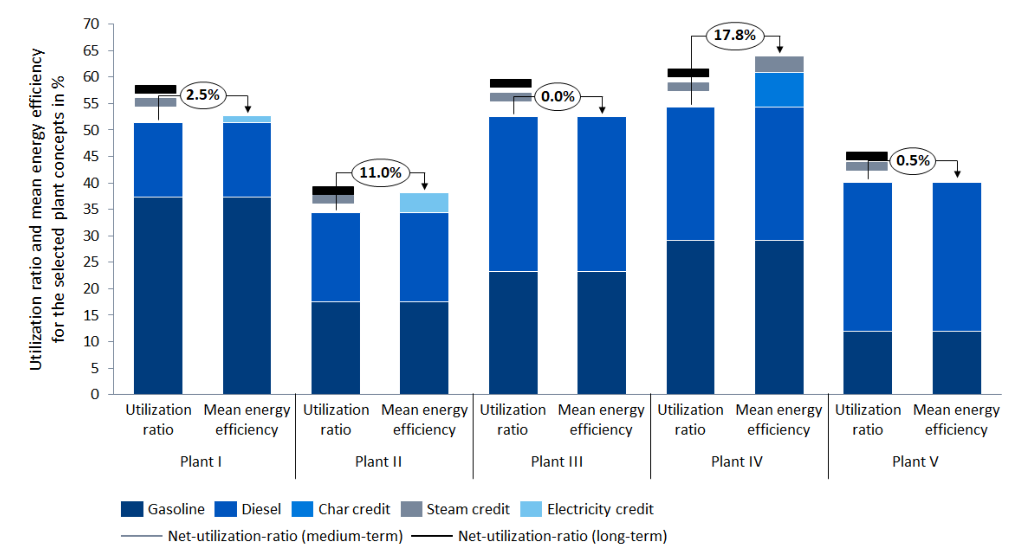
- Plant I. Diesel and gasoline are produced via in situ fast pyrolysis and catalytic vapor upgrading and downstream processing including hydro-treating. As a result, the utilization ratio of the process is 51% for the current status. In comparison with the other plant concepts, this concept produces 27% diesel compared to gasoline. The mean energy efficiency is 53% and, thus, it is slightly higher compared to the average energy efficiency of the five plant concepts (50%). Plant I utilizes 0.01 MJ per kg of diesel as well as of natural gas. The electricity credit is around 0.22 MJ/kg.
- Plant II. This plant concept produces via fast pyrolysis and subsequent slurry upgrading, including Fischer–Tropsch (FT) synthesis ~49% diesel compared to gasoline. The calculated utilization ratio of 34% is lower compared to the average value of the plant concepts (47%). The mean fuel efficiency is 38% and, thus, it is slightly lower compared to the average energy efficiency. The electricity credit is the highest of all plant concepts with around 0.67 MJ/kg.
- Plant III. The utilization ratio of the fast pyrolysis and liquid upgrading plant is 52%, as is the mean fuel efficiency. This plant concept produces 56% diesel. The electricity use is ~0.44 MJ/kg, and the natural gas use is the second highest with 2.08 MJ/kg.
- Plant IV. This plant concept of fast pyrolysis and liquid upgrading has the highest energy needs for electricity and natural gas with 1.52 MJ/kg and 3.28 MJ/kg, resectively. The plant produces 46% diesel. Credit can be given for 1.57 MJ/kg of char and 0.75 MJ/kg of steam.
- Plant V. Compared to the fast pyrolysis concepts, the gasification and Fischer–Tropsch (FT) synthesis concept gains yields of 40% utilization ratio and up to 43% mean energy efficiency. This plant concept produces 70% diesel. The electricity credit is 0.60 MJ/kg.
Medium- and Long-Term Perspective
- In plant I, diesel and gasoline are produced via in situ fast pyrolysis and catalytic vapor upgrading and downstream processing including hydro-treating. As a result, the utilization ratio of the process ranges between 55% and 58% for the medium- and long-term.
- Plant II produces via fast pyrolysis and subsequent slurry upgrading, including Fischer–Tropsch (FT) synthesis ~49% diesel compared to gasoline. The utilization ratio, 37% to 39%, is lower compared to the average value of the plant concepts.
- The utilization ratio of plant III of the fast pyrolysis and liquid upgrading plant is between 56% and 59%.
- Plant IV, with fast pyrolysis and liquid upgrading, has a utilization ratio for the medium- and long-term between 58% and 61%.
- Plant V, compared to the fast pyrolysis concepts, the gasification and Fischer–Tropsch synthesis concept has a utilization ratio for medium- and long-term perspectives between 43% and 45%.
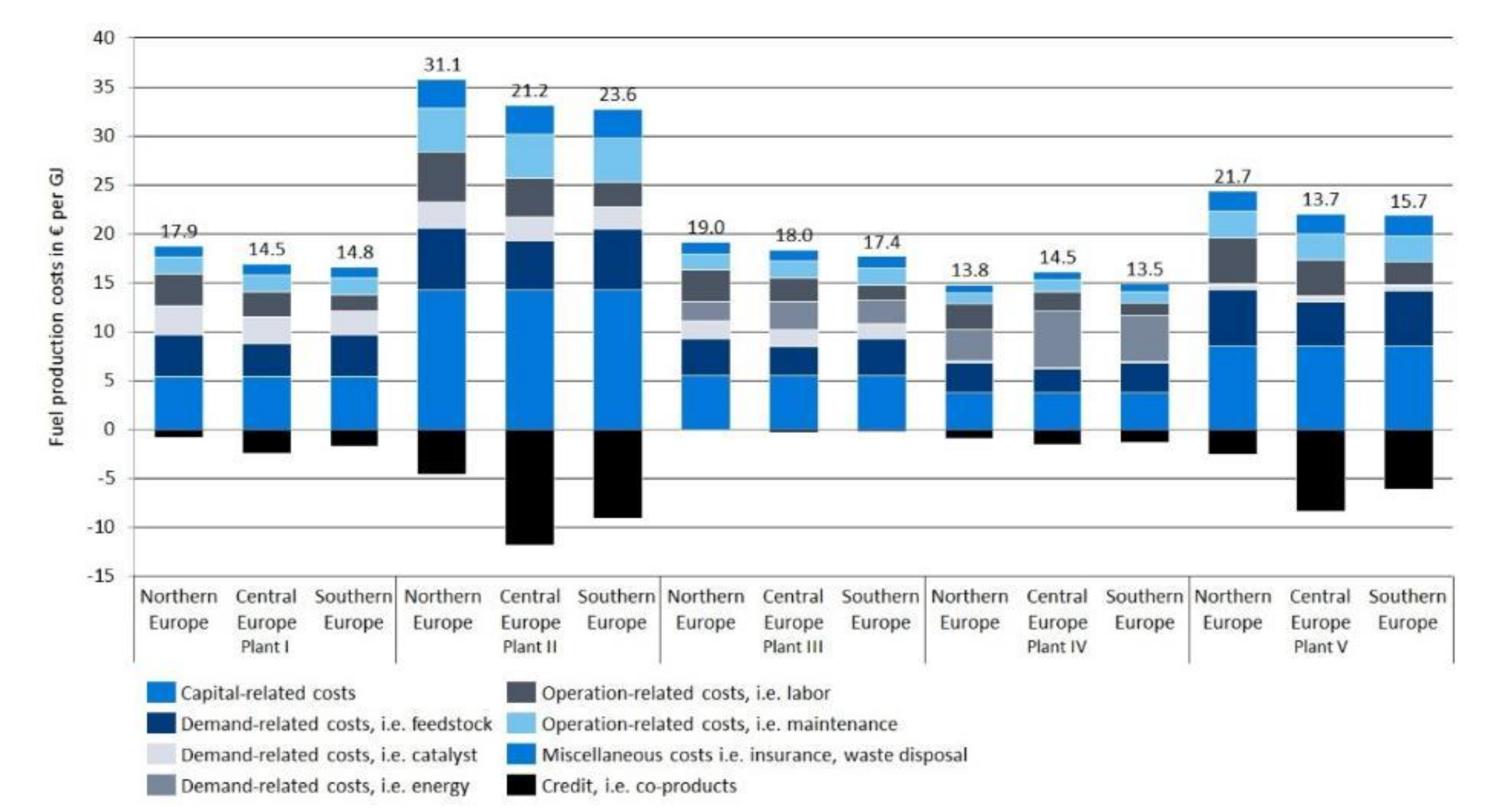
3.3.2. Economic Assessment
Current Status
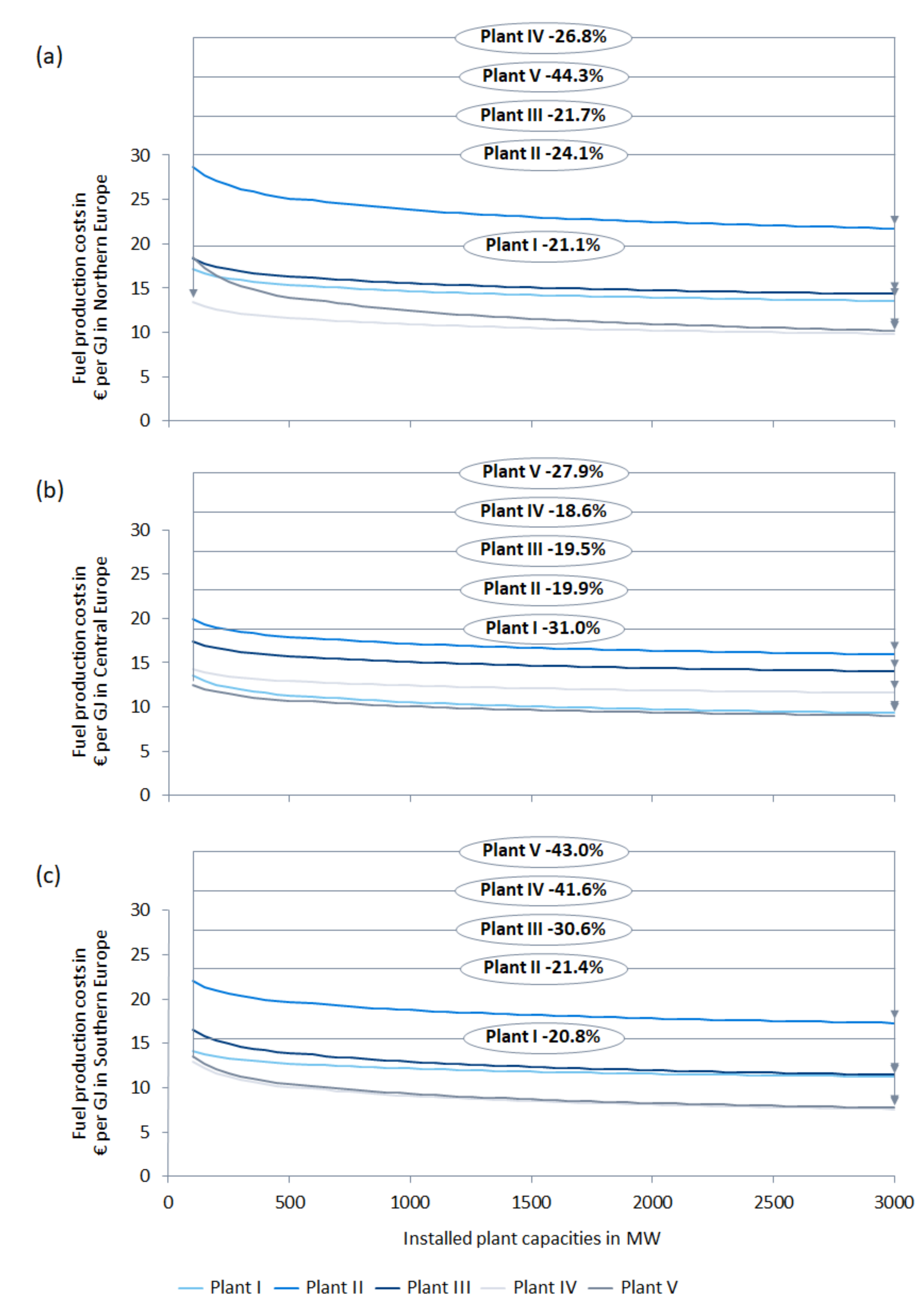
Medium- and Long-Term Perspective
3.3.3. Environmental Assessment
Current Status
Medium- and Long-Term Perspectives
4. Discussion and Conclusions
- Utilization ratio and energy efficiency. Clear differences in the utilization ratio for the plant concepts become obvious. Plant concepts I, III, and IV achieve a utilization ratio of more than 50%, whereas plant concepts II and V have a significantly lower utilization ratio. Similar trends can be observed with regard to mean energy efficiency. Plant concept IV, achieving a significant increase in efficiency due to the co-products, is particularly notable.
- Costs. Four out of five plant concepts, no matter in which location, have a negative net income value, except for Plant IV, resulting in a positive value in northern Europe (344 k€/a) and in southern Europe (884 k€/a). Therefore, according to current data, it can be assumed that no profitable production of intermediate biogenic products for the chemical industry is currently possible. In the medium- and long-term, however, with a strong increase in installed plant capacities, it can be assumed that the production of intermediate biogenic products can definitely make a cost-effective contribution to the chemical industry, assuming there is a strong increase in CO2-taxes and thus a clear price increase for fossil fuel energy.
- Environmental impact. Among other things, plant concepts I and V show lower values than plant concepts III and IV, as the catalysts have a significantly lower replacement rates per year.
Supplementary Materials
Author Contributions
Funding
Institutional Review Board Statement
Informed Consent Statement
Data Availability Statement
Acknowledgments
Conflicts of Interest
References
- European Commission. The European Green Deal; European Commission: Brussels, Belgium, 2019. [Google Scholar]
- European Commission. A New Circular Economy Action Plan for a Cleaner and More Competitive Europe; European Commission: Brussels, Belgium, 2019. [Google Scholar]
- European Commission. Bioeconomy: The European Way to Use Our Natural Resources: Action Plan 2018; European Commission: Brussels, Belgium, 2018; ISBN 978-92-79-85245-9. [Google Scholar]
- Carus, M. Biobased Economy and Climate Change—Important Links, Pitfalls, and Opportunities. Ind. Biotechnol. 2017, 13, 41–51. [Google Scholar] [CrossRef]
- Gelfand, I.; Sahajpal, R.; Zhang, X.; Izaurralde, R.C.; Gross, K.L.; Robertson, G.P. Sustainable Bioenergy Production from Marginal Lands in the US Midwest. Nature 2013, 493, 514–517. [Google Scholar] [CrossRef] [PubMed]
- Mast, B. Sustainable Bioenergy Cropping Concepts—Optimizing Biomass Provision for Different Conversion Routes. Ph.D. Thesis, Faculty of Agricultural Sciences, University of Hohenheim, Hohenheim, Germany, 2014. [Google Scholar]
- Zhou, C. Gasification and Pyrolysis Characterization and Heat Transfer Phenomena during Thermal Conversion of Municipal Solid Waste; Industrial Engineering and Management, KTH Royal Institute of Technology: Stockholm, Sweden, 2014; ISBN 978-91-7595-284-0. [Google Scholar]
- Cascatbel. D10.5 Highlights of CASCATBEL’s Annual Progress for Public Dissemination. 2014. Available online: http://www.cascatbel.eu/wp-content/uploads/D10.5-Annual-public-highlihts-first-year1.pdf (accessed on 20 February 2021).
- Baumbach, G.; Hartmann, H.; Höfer, I.; Hofbauer, H.; Hülsmann, T.; Kaltschmitt, M.; Lenz, V.; Neuling, U.; Nussbaumer, T.; Obernberger, I.; et al. Grundlagen der thermo-chemischen Umwandlung biogener Festbrennstoffe. In Energie aus Biomasse; Kaltschmitt, M., Hartmann, H., Hofbauer, H., Eds.; Springer Vieweg: Berlin Heidelberg, Germany, 2016; pp. 579–814. ISBN 978-3-662-47437-2. [Google Scholar]
- Hornung, A. Influence of Feedstocks on Performance and Products of Processes. In Transformation of Biomass; Hornung, A., Ed.; John Wiley & Sons, Ltd.: Chichester, UK, 2014; pp. 203–207. ISBN 978-1-118-69364-3. [Google Scholar]
- Wi, S.G.; Cho, E.J.; Lee, D.-S.; Lee, S.J.; Lee, Y.J.; Bae, H.-J. Lignocellulose Conversion for Biofuel: A New Pretreatment Greatly Improves Downstream Biocatalytic Hydrolysis of Various Lignocellulosic Materials. Biotechnol. Biofuels 2015, 8, 228. [Google Scholar] [CrossRef] [PubMed] [Green Version]
- Dees, M.; Elbersen, B.; Fitzgerald, J.; Vis, M.; Anttila, P.; Forsell, N.; Ramirez-Almeyda, J.; García Galindo, D.; Glavonjic, B.; Staritsky, I.; et al. A Spatial Data Base on Sustainable Biomass Cost-Supply of Lignocellulosic Biomass in Europe—Methods & Data Sources: Project Report. S2BIOM—A Project Funded under the European Union 7th Frame Programme. Grant Agreement N°608622. 2016. Available online: https://www.s2biom.eu/images/Publications/D1.6_S2Biom_Spatial_data_methods_data_sources_Final_Final.pdf (accessed on 31 August 2021).
- European Commission. Modal Split of Inland Freight Transport in 2015; Statistical Pocketbook; Publications Office of the European Union: Luxembourg, 2016; ISBN 978-92-79-51528-6. [Google Scholar]
- Hartmann, H.; Kaltschmitt, M.; Thrän, D.; Wirkner, R. Bereitstellungskonzepte. In Energie aus Biomasse; Kaltschmitt, M., Hartmann, H., Hofbauer, H., Eds.; Springer Vieweg: Berlin/Heidelberg, Germany, 2016; pp. 325–382. ISBN 978-3-662-47437-2. [Google Scholar]
- VDI. VDI 6310 Classification and Quality Criteria of Biorefineries; The Association of German Engineers (VDI): Düsseldorf, Germany, 2016. [Google Scholar]
- Meriam, J.L.; Kraige, L.G. Engineering Mechanics, 3rd ed.; Wiley: New York, NY, USA; Chichester, UK, 1993; ISBN 978-0-471-59273-0. [Google Scholar]
- Bridgwater, A.V.; Toft, A.J.; Brammer, J.G. A Techno-Economic Comparison of Power Production by Biomass Fast Pyrolysis with Gasification and Combustion. Renew. Sustain. Energy Rev. 2002, 6, 181–246. [Google Scholar] [CrossRef]
- Mitchell, C.P.; Bridgwater, A.V.; Stevens, D.J.; Toft, A.J.; Watters, M.P. Technoeconomic Assessment of Biomass to Energy. Int. Energy Agency Bioenergy Agreem. Prog. Achiev. 1995, 9, 205–226. [Google Scholar] [CrossRef]
- Hall, P.; Hock, B.; Nicholas, I. Volume and Cost Analysis of Large Scale Woody Biomass Supply: Southland and Central North Island. In Report for the Parliamentary Commissioner for the Environment; SCION: Rotorua, New Zealand, 2010. [Google Scholar]
- Hall, P.; Jack, M. Bioenergy Options for New Zealand–Analysis of Large-Scale Bioenergy from Forestry; SCION: Rotorua, New Zealand, 2009. [Google Scholar]
- ISO. ISO 16290:2016-09, Space Systems—Definition of the Technology Readiness Levels (TRLs) and Their Criteria of Assessment, (ISO_16290:2013); International Organization for Standardization (ISO): Geneva, Switzerland, 2013. [Google Scholar]
- NASA. Technology Readiness Levels. 2015. Available online: https://www.nasa.gov/directorates/heo/scan/engineering/technology/technology_readiness_level/ (accessed on 1 March 2020).
- NASA. Technology Readiness Level Definitions. 2017. Available online: https://www.innovation.cc/discussion-papers/2017_22_2_3_heder_nasa-to-eu-trl-scale.pdf (accessed on 1 March 2020).
- Vauck, W.R.A.; Müller, H.A. Grundoperationen Chemischer Verfahrenstechnik, 11th ed.; Deutscher Verlag für Grundstoffindustrie: Stuttgart, Germany, 2000; ISBN 978-3-342-00687-9. [Google Scholar]
- Müller-Erlwein, E. Chemische Reaktionstechnik, 2nd ed.; B.G. Teuber Verlag: Leipzig, Germany; GWV Fachverlage GmbH: Wiesbaden, Germany, 2007; ISBN 978-3-8351-9097-9. [Google Scholar]
- Smith, R. Chemical Process Design: For the Efficient Use of Resources and Reduced Environmental Impact, 2nd ed.; Wiley: Chichester, UK, 2005; ISBN 0-471-48681-7. [Google Scholar]
- Pérez, C. Technological Change and Opportunities for Development as a Moving Target. CEPAL 2001, 75, 109–130. [Google Scholar] [CrossRef]
- Weidema, I. New Developments in the Methodology for LCA. In Proceedings of the 3rd International Conference on Ecobalance, Tsukuba City, Japan, 25–27 November 1998. [Google Scholar]
- Perez, C. Technological Revolutions and Techno-Economic Paradigms. Camb. J. Econ. 2010, 34, 185–202. [Google Scholar] [CrossRef] [Green Version]
- Mertens, P. Mittel- und langfristige Absatzprognose auf der Basis von Sättigungsmodellen. In Prognoserechnung; Mertens, P., Rässler, S., Eds.; Physica-Verlag HD: Heidelberg, Germany, 2012; pp. 183–224. ISBN 978-3-7908-2796-5. [Google Scholar]
- Kucharavy, D.; de Guio, R. Application of S-Shaped Curves. Procedia Eng. 2011, 9, 559–572. [Google Scholar] [CrossRef] [Green Version]
- Taheri, A.; Cavallucci, D.; Oget, D. Positioning Ideality in Inventive Design; Distinction, Characteristics, Measurement. In Proceedings of the 2014 International Conference on Engineering, Technology and Innovation (ICE), Bergamo, Italy, 23–25 June 2014; pp. 1–6. [Google Scholar] [CrossRef]
- VDI. VDI 2067 Economic Efficiency of Building Installations—Fundamentals and Economic Calculation; The Association of German Engineers (VDI): Düsseldorf, Germany, 2012. [Google Scholar]
- Peters, M.S.; Timmerhaus, K.D.; West, R.E. Plant Design and Economics for Chemical Engineers, 5th ed.; McGraw-Hill Chemical Engineering Series; McGraw-Hill: Boston, MA, USA, 2006; ISBN 978-0-07-239266-1. [Google Scholar]
- Mussatti, D.; Vatavuk, W. Cost Estimation: Concepts and Methodology; U.S. Environmental Protection Agency: Research Triangle Park, NC, USA, 2002.
- Dutta, A.; Sahir, A.; Tan, E.; Humbird, D.; Snowden-Swan, L.; Meyer, P.; Ross, J.; Sexton, D.; Yap, R.; Lukas, J. Process Design and Economics for the Conversion of Lignocellulosic Biomass to Hydrocarbon Fuels: Thermochemical Research Pathways with In Situ and Ex Situ Upgrading of Fast Pyrolysis Vapors; Colorado; U.S. Department of Energy: Washington, DC, USA, 2015.
- Remmers, J. Zur Ex-Ante-Bestimmung von Investitionen Bzw. Kosten Für Emissionsminderungstechniken Und Den Auswirkungen Der Datenqualität in Meso-Skaligen Energie-Umwelt-Modellen. Ph.D. Thesis, Karlsruhe University, Karlsruhe, Germany, 1991. [Google Scholar]
- Lang, H.J. Cost Relationships in Preliminary Cost Estimation. Chem. Eng 1947, 54, 27. [Google Scholar]
- Couper, J.R. Process Engineering Economics; Chemical Industries Ser; Taylor & Francis Group: Philadelphia, PA, USA, 2003; Volume 97, ISBN 978-0-8247-4036-8. [Google Scholar]
- United States Department of Labor Databases, Tables & Calculators: Producer Price Index-Commodities. Chemicals and Allied Products. Basic Inorganic Chemicals. Available online: https://data.bls.gov/timeseries/WPU0613?output_view=pct_3mths (accessed on 9 August 2020).
- Desroches, L.-B.; Garbesi, K.; Kantner, C.; van Buskirk, R.; Yang, H.-C. Incorporating Experience Curves in Appliance Standards Analysis. Energy Policy 2013, 52, 402–416. [Google Scholar] [CrossRef] [Green Version]
- Pignataro, P. Financial Modeling and Valuation: A Practical Guide to Investment Banking and Private Equity; Wiley Finance Series; Wiley: Hoboken, NJ, USA, 2013; ISBN 978-1-118-55876-8. [Google Scholar]
- Farris, P.W. (Ed.) Marketing Metrics: The Definitive Guide to Measuring Marketing Performance, 2nd ed.; FT Press: Upper Saddle River, NJ, USA, 2010; ISBN 978-0-13-705829-7. [Google Scholar]
- Larsen, H.F.; von der Voet, E.; van Oers, L.; Yang, G.; Rydberg, T. Life Cycle Assessment and Additives: State of Knowledge, In Proceedings of 2nd RISKCYCLE Workshop: Risk of Chemical Additives and Recycled Materials, Dresden, Germany, 8–9 May 2012.
- ISO. ISO 14040Environmental Management—Life Cycle Assessment—Principles and Framework, International Organization for Standardization (ISO); Beuth Verlag: Berlin, Germany, 2006; Volume 2006. [Google Scholar]
- ISO. ISO 14044 Environmental Management—Life Cycle Assessment—Requirements and Guidelines; International Organization for Standardization (ISO): Geneva, Switzerland, 2006. [Google Scholar]
- Argonne National Laboratory. Summary of Expansions, Updates, and Results in GREET® 2016 Suite of Models; Argonne National Laboratory: Lemont, IL, USA, 2016. [Google Scholar] [CrossRef]
- Frischknecht, R.; Jungbluth, N.; Althaus, H.-J.; Doka, G.; Dones, R.; Heck, T.; Hellweg, S.; Hischier, R.; Nemecek, T.; Rebitzer, G.; et al. The ecoinvent database: Overview and methodological framework. Int. J. Life Cycle Assess. 2005, 10, 3–9. [Google Scholar] [CrossRef]
- Tillman, A.-M. Significance of Decision-Making for LCA Methodology. Environ. Impact Assess. Rev. 2000, 20, 113–123. [Google Scholar] [CrossRef] [Green Version]
- European Commission. International Reference Life Cycle Data System (ILCD) Handbook: General Guide on LCA—Detailed Guidance; European Commission: Brussels, Belgium, 2010. [Google Scholar]
- Christensen, T.H. (Ed.) Solid Waste Technology & Management; Wiley and Wiley Blackwell: Chichester, UK, 2011; ISBN 978-1-4051-7517-3. [Google Scholar]
- Torres, C.M.; Gadalla, M.; Mateo-Sanz, J.M.; Jiménez, L. An Automated Environmental and Economic Evaluation Methodology for the Optimization of a Sour Water Stripping Plant. J. Clean. Prod. 2013, 44, 56–68. [Google Scholar] [CrossRef]
- Klöpffer, W.; Grahl, B. Ökobilanz (LCA): Ein Leitfaden Für Ausbildung Und Beruf; Wiley-VCH: Weinheim, Germany, 2009; ISBN 978-3-527-32043-1. [Google Scholar]
- Weinberg, J. Die Zukünftige Entwicklung Der Straßengebundenen Mobilität in Deutschland. PhD Thesis, Hamburg University of Technology, Hamburg, Germany, 2014. [Google Scholar]
- Börjeson, L.; Höjer, M.; Dreborg, K.-H.; Ekvall, T.; Finnveden, G. Scenario Types and Techniques: Towards a User’s Guide. Futures 2006, 38, 723–739. [Google Scholar] [CrossRef]
- Peters, J. Pyrolysis for Biofuels or Biochar? A Thermoynamic, Environmental and Economic Assessment. Ph.D. Thesis, Universidad Rey Juan Carlos, Móstoles, Madrid, 2015. [Google Scholar]
- Jones, S.; Snowden-Swan, L.J.; Meyer, P.; Zacher, A.H.; Olarte, M.; Wang, H.; Drennan, C. Fast Pyrolysis and Hydrotreating: 2015 State of Technology R&D and Projections to 2017; U.S. Department of Energy, Pacific Northwest National Laboratory: Richland, WA, USA, 2016.
- Jones, S.B.; Valkenburg, C.; Walton, C.W.; Elliott, D.C.; Holladay, J.E.; Stevens, D.J.; Kinchin, C.; Czernik, S. Production of Gasoline and Diesel from Biomass via Fast Pyrolysis, Hydrotreating and Hydrocracking: A Design Case; U.S. Department of Energy: Washington, DC, USA, 2009.
- Trippe, F. Techno-Ökonomische Bewertung Alternativer Verfahrenskonfigurationen Zur Herstellung von Biomass-to-Liquid (BtL) Kraftstoffen Und Chemikalien. Ph.D. Thesis, Karlsruhe Institute of Technology, Karlsruhe, Germany, 2013. [Google Scholar]
- Jones, S.; Meyer, P.; Snowden-Swan, L.; Tan, E.; Dutta, A.; Jacobsen, J.; Cafferty, K. Process Design and Economics for the Conversion of Lignocellulosic Biomass to Hydrocarbon Fuels: Fast Pyrolysis and Hydrotreating Bio-Oil Pathway; U.S. Department of Energy Bioenergy Technologies Office: Washington, DC, USA, 2013.
- Swanson, R.M.; Platon, A.; Satrio, J.A.; Brown, R.C.; Hsu, D.D. Techno-Economic Analysis of Biofuels Production Based on Gasification; National Renewable Energy Laboratory: Golden, CO, USA, 2010.
- Kaltschmitt, M. (Ed.) Erneuerbare Energien: Systemtechnik, Wirtschaftlichkeit, Umweltaspekte, 5th ed.; Springer: Berlin, Germany, 2014; ISBN 978-3-642-03249-3. [Google Scholar]
- Daugaard, T.; Mutti, L.A.; Wright, M.M.; Brown, R.C.; Componation, P. Learning Rates and Their Impacts on the Optimal Capacities and Production Costs of Biorefineries. Biofuels Bioprod. Biorefining 2015, 9, 82–94. [Google Scholar] [CrossRef]
- International Renewable Energy Agency. Innovation Outlook: Advanced Liquid Biofuels; IRENA: Masdar City, United Arab Emirates, 2016; ISBN 978-92-95111-51-6. [Google Scholar]
- Rosenqvist, H.; Berndes, G.; Börjesson, P. The Prospects of Cost Reductions in Willow Production in Sweden. Biomass Bioenergy 2013, 48, 139–147. [Google Scholar] [CrossRef]
- Detz, R.J.; Reek, J.N.H.; Zwaan, B.C.C. The Future of Solar Fuels: When Could They Become Competitive? Energy Environ. Sci. 2018, 11, 1653–1669. [Google Scholar] [CrossRef]
- White, R. A Techno-Economic, Sustainability and Experimental Assessment of the Direct Methanation of Biodiesel Waste Glycerol. Ph.D. Thesis, Energy Research Institute, School of Chemical and Process Engineering, The University of Leeds, Leeds, UK, 2018. [Google Scholar]
- Sanchez, R. DOE G 413.3-21. In Cost Estimating Guide; U.S. Department of Energy: Washington, DC, USA, 2011. [Google Scholar]
- Han, J.; Elgowainy, A.; Dunn, J.B.; Wang, M.Q. Life Cycle Analysis of Fuel Production from Fast Pyrolysis of Biomass. Bioresour. Technol. 2013, 133, 421–428. [Google Scholar] [CrossRef] [PubMed]
- Menten, F.; Chèze, B.; Patouillard, L.; Bouvart, F. A Review of LCA Greenhouse Gas Emissions Results for Advanced Biofuels: The Use of Meta-Regression Analysis. Renew. Sustain. Energy Rev. 2013, 26, 108–134. [Google Scholar] [CrossRef]
- Muench, S.; Guenther, E. A Systematic Review of Bioenergy Life Cycle Assessments. Appl. Energy 2013, 112, 257–273. [Google Scholar] [CrossRef]
- Benavides, P.T.; Dai, Q.; Sullivan, J.; Kelly, J.C.; Dunn, J. Material and Energy Flows Associated with Select Metals in GREET2: Molybdenum, Platinum, Zinc, Nickel, Silicon: ANL/ESD-15/11; Argonne National Laboratory: Lemont, IL, USA, 2015. [Google Scholar]
- Dai, Q.; Kelly, J.C.; Burnham, A.; Elgowainy, A. Updated Life-Cycle Analysis of Aluminum Production and Semi-Fabrication for the GREET Model; Energy Systems Division, Argonne National Laboratory: Lemont, IL, USA, 2015. [Google Scholar]
- Dias, A.C. Life Cycle Assessment of Fuel Chip Production from Eucalypt Forest Residues. Int. J. Life Cycle Assess. 2014, 19, 705–717. [Google Scholar] [CrossRef]
- Eurostat. Database: Your Key to European Statistics; Statistical Office of the European Communities, European Commission: Brussels, Belgium, 2019. [Google Scholar]
- Jin, E. Life Cycle Assessment of Two Catalysts Used in the Biofuel Syngas Cleaning Process and Analysis of Variability in Gasification. Master’s Thesis, Oklahoma State University, Stillwater, OK, USA, 2014. [Google Scholar]
- Khoo, H.H.; Ee, W.L.; Isoni, V. Bio-Chemicals from Lignocellulose Feedstock: Sustainability, LCA and the Green Conundrum. Green Chem. 2016, 18, 1912–1922. [Google Scholar] [CrossRef]
- Xie, X.; Wang, M.; Han, J. Assessment of Fuel-Cycle Energy Use and Greenhouse Gas Emissions for Fischer-Tropsch Diesel from Coal and Cellulosic Biomass. Environ. Sci. Technol. 2011, 45, 3047–3053. [Google Scholar] [CrossRef] [PubMed]
- Wang, M.; Han, J.; Dunn, J.B.; Cai, H.; Elgowainy, A. Well-to-Wheels Energy Use and Greenhouse Gas Emissions of Ethanol from Corn, Sugarcane and Cellulosic Biomass for US Use. Environ. Res. Lett. 2012, 7, 045905. [Google Scholar] [CrossRef] [Green Version]
- Spatari, S.; Larnaudie, V.; Mannoh, I.; Wheeler, M.C.; Macken, N.A.; Mullen, C.A.; Boateng, A.A. Environmental, Exergetic and Economic Tradeoffs of Catalytic- and Fast Pyrolysis-to-Renewable Diesel. Renew. Energy 2020, 162, 371–380. [Google Scholar] [CrossRef]
- Sorunmu, Y.; Billen, P.; Spatari, S. A Review of Thermochemical Upgrading of Pyrolysis Bio-Oil: Techno-Economic Analysis, Life Cycle Assessment, and Technology Readiness. GCB Bioenergy 2020, 12, 4–18. [Google Scholar] [CrossRef] [Green Version]
- Gupta, S.; Mondal, P.; Borugadda, V.B.; Dalai, A.K. Advances in Upgradation of Pyrolysis Bio-Oil and Biochar towards Improvement in Bio-Refinery Economics: A Comprehensive Review. Environ. Technol. Innov. 2021, 21, 101276. [Google Scholar] [CrossRef]
- Elia, A.; Kamidelivand, M.; Rogan, F.; Gallachóir, B.Ó. Impacts of Innovation on Renewable Energy Technology Cost Reductions. Renew. Sustain. Energy Rev. 2021, 138, 110488. [Google Scholar] [CrossRef]
- Grafström, J.; Poudineh, R. A Critical Assessment of Learning Curves for Solar and Wind Power Technologies; The Oxford Institute of Energy: Oxford, UK, 2021; ISBN 978-1-78467-172-3. [Google Scholar]


| Level | Definition | Qualifying Criteria |
|---|---|---|
| 1 | Observation and reporting of fundamental principles | Peer-reviewed publication of research relevant to the proposed concept/application |
| 2 | Formulation of technology concept and application | Documented description of the application concept addressing feasibility and benefit |
| 3 | Analytical and experimental critical function and characteristic verification of concept | Documented analytical and experimental results validating predictions of key performance parameters |
| 4 | Component and breadboard proof in a laboratory environment | Documented test performance demonstrating consensus with analytical predictions; documented definition of relevant environment |
| 5 | Component and breadboard proof in relevant environment | Documented test performance demonstrating consensus with analytical predictions; documented definition of scaling requirements |
| 6 | System/sub-system model or prototype demonstration in an operational environment | Documented test performance demonstrating consensus with analytical predictions |
| 7 | System prototype demonstration in an operational environment | Documented test performance demonstrating consensus with analytical predictions |
| 8 | Actual system completed and qualified through test and demonstration | Documented test performance verifying analytical predictions |
| 9 | Actual system proven through successful operations | Documented operational results |
| Parameter | Unit | Northern Europe | Central Europe | Southern Europe |
|---|---|---|---|---|
| Country | Sweden | Germany | Spain | |
| Location | Skåne Iän | Mecklenburgische Seenplatte | Ciudad Real | |
| NUTS-3-region | SE224 | DE80 J | ES422 | |
| NUTS-3 area | km2 | 11,302 | 5468 | 19,813 |
| Forestry residues 1 | tn. l.DM/a | 35,071 | 24,881 | 6143 |
| Agricultural residues | tn. l.DM/a | 112,177 | 123,105 | 40,914 |
| Energy crops | tn. l.DM/a | 193 | 199 | 102,434 |
| Sum | tn. l.DM/a | 147,442 | 148,185 | 149,492 |
| Parameter | Unit | Northern Europe | Central Europe | Southern Europe |
|---|---|---|---|---|
| Annual available lignocellulosic biomass | MJ/km2 | 5,109,743 | 4,964,876 | 3,387,719 |
| Transportation on unsealed road 1 | km | 27.3 | 28.4 | 39.5 |
| Transportation distance on sealed road | km | 4.8 | 5.0 | 7.0 |
| Sum | km | 32.2 | 33.4 | 46.5 |
| Unit | Plant I | Plant II | Plant III | Plant IV | Plant V | |
|---|---|---|---|---|---|---|
| Yield of gasoline 1 | L/tDM | 191.6 | 89.6 | 137.0 | 208.1 | 63.0 |
| Yield of diesel 2 | L/tDM | 63.5 | 85.1 | 150.1 | 158.2 | 130.7 |
| Fuel produced | m3/a | 42,188 | 28,893 | 47,469 | 60,564 | 32,015 |
| Diesel percentage | % | 27 | 49 | 56 | 46 | 70 |
| Yield of electricity | kWh/tDM | 795.8 | 2424.6 | 0 | 0 | 2148.5 |
| Electricity required 3 | kWh/tDM | 0 | 0 | 122.45 | 422.10 | 0 |
| Natural gas required | GJ/tDM | 0.01 | 0 | 2.08 | 3.28 | 0.09 |
| Yield of co-product 4 | €/tDM | 2.5 | 0 | 0 | 9.6 | 9.4 |
| Unit | Plant I | Plant II | Plant III | Plant IV | Plant V | |
|---|---|---|---|---|---|---|
| Shifts | per day | 3 | 3 | 3 | 3 | 3 |
| Production labor | per shift | 11.0 | 10.8 | 15.5 | 13.0 | 14.0 |
| Chargehand labor | per shift | 4.1 | 3.8 | 2.1 | 4.0 | 3.1 |
| Specialist labor | per shift | 0.5 | 1.8 | 0.5 | 1.0 | 0.5 |
| Office staff | per year | 1 | 1 | 1 | 1 | 1 |
| Management staff | per year | 1 | 1 | 1 | 1 | 1 |
| Plant I | Plant II | Plant III | Plant IV | Plant V | |
|---|---|---|---|---|---|
| Capital related costs | 0.08 | 0.05–0.15 | |||
| Demand related costs | |||||
| Feedstock | 0.00 1–0.05 2 | 0.05 | |||
| Catalyst | 0.01 | 0.04–0.06 | |||
| Energy | 0 | ||||
| Operating related costs | |||||
| Labor | 0.075 | ||||
| Maintenance | 0.05 | 0.1 | |||
| Miscellaneous costs | 0.051 | ||||
| Unit | Plant I | Plant II | Plant III | Plant IV | Plant V | |
|---|---|---|---|---|---|---|
| Northern Europe | ||||||
| Net sales | k€/a | 18,162 | 84,205 | 22,813 | 30,849 | 12,186 |
| Net income | k€/a | −82,086 | −23,901 | −75,061 | 344 | −12,911 |
| Central Europe | ||||||
| Net sales | k€/a | 14,227 | −913 | 20,888 | 29,642 | 3190 |
| Net income | k€/a | −9120 | −30,276 | −8027 | −3706 | −19,026 |
| Southern Europe | ||||||
| Net sales | k€/a | 17,136 | 3505 | 22,890 | 31,853 | 7426 |
| Net income | k€/a | −5761 | −25,448 | −4771 | 884 | −14,574 |
Publisher’s Note: MDPI stays neutral with regard to jurisdictional claims in published maps and institutional affiliations. |
© 2021 by the authors. Licensee MDPI, Basel, Switzerland. This article is an open access article distributed under the terms and conditions of the Creative Commons Attribution (CC BY) license (https://creativecommons.org/licenses/by/4.0/).
Share and Cite
Thormann, L.; Neuling, U.; Kaltschmitt, M. Opportunities and Challenges of the European Green Deal for the Chemical Industry: An Approach Measuring Innovations in Bioeconomy. Resources 2021, 10, 91. https://0-doi-org.brum.beds.ac.uk/10.3390/resources10090091
Thormann L, Neuling U, Kaltschmitt M. Opportunities and Challenges of the European Green Deal for the Chemical Industry: An Approach Measuring Innovations in Bioeconomy. Resources. 2021; 10(9):91. https://0-doi-org.brum.beds.ac.uk/10.3390/resources10090091
Chicago/Turabian StyleThormann, Lisa, Ulf Neuling, and Martin Kaltschmitt. 2021. "Opportunities and Challenges of the European Green Deal for the Chemical Industry: An Approach Measuring Innovations in Bioeconomy" Resources 10, no. 9: 91. https://0-doi-org.brum.beds.ac.uk/10.3390/resources10090091