
Long-Term Sustainability of Copper and Iron Based on a System Dynamics Model


Department of Geosciences, Geotechnology and Materials Engineering for Resources, Akita University, 1-1 Tegata Gakuen-Cyou, Akita 010-8502, Japan
*
Author to whom correspondence should be addressed.
Resources 2022, 11(4), 37; https://0-doi-org.brum.beds.ac.uk/10.3390/resources11040037
Submission received: 2 March 2022
/
Revised: 1 April 2022
/
Accepted: 1 April 2022
/
Published: 6 April 2022
(This article belongs to the Collection Management, Environment, Energy and Sustainability under a Circular Economy)
Abstract
:Copper and iron are critical to the economic growth of modern society. Nations depend on these metals for the development of infrastructure, transportation, and other industries. However, concerns regarding future availability of “peak minerals” with a “limit to growth” have been extensively debated. The purpose of this study was to investigate the amount of potential resources and the recycling rate from secondary metal scrap recycling for the sustainable development of mineral resources. The long-term mineral supply and demand balance with respect to recycling for copper and iron were developed for the next 50 years at the regional and global levels. The results indicate that the supply of copper would increase four-fold by 2070 compared to 1991, with primary copper remaining the main contributing source. For iron, the total supply would increase by nine times from 2000 to 2070, with secondary recycling surpassing the primary iron supply by 2033 and becoming the main contributor by 2070. Even though there is no future resource constraint, further promotion of scrap recycling, especially for copper, is necessary to address environmental concerns through reduction in material extraction. Emphasizing the importance of metals in society is essential for stock accountability through resource efficiency and resource conservation.
1. Introduction
Copper and iron are ubiquitous in the products we use today. Owing to their unique properties, these metals have proven to be essential components of transport, building, and construction. The demand for copper and iron has increased exponentially as a result of the increasing per capita income of nations. This demand is expected to grow by 3.2% annually [1,2]. The rising scale of production in copper and iron ore mining raise concerns about their future availability, with regard to their “limit to growth.” The pertinent question is whether this may become a problem for long-term physical availability [3,4,5,6,7,8,9,10,11].
Several attempts have been made earlier to model trends in metal production. The Hubbert function, comprising the ultimate recoverable reserves (URR), has been used to assess metal mining rates to estimate when production will peak [12]. Adachi et al. developed a long-term global copper supply and demand model using system dynamics to allocate 12 regions as primary copper producers, and the final demand was measured taking into account recycling and metal substitution [13]. The study made strong assumptions based on geological constraints in their analysis, and the results indicated that a strong promotion in recycling is required to satisfy copper demand. Van Vuuren et al. outlined the principles of global metal cycles for copper by applying system dynamics to simulate mineral consumption up to the year 2100 by considering ore-grade decline, capital, energy requirements, and waste flows in their modelling [1]. The mineral resources were characterized as abundant or scarce. The production cost was expressed as a function of energy consumption to investigate the sustainability concerns of metal resource use. Ayres et al. applied time series supply and demand for copper lifecycle up to 2100 at a global level and specifically for the United States [14]. Their model involved material balancing in the “Intergovernmental Panel on Climate Change Special Report on Emission Scenario B (IPCC-SRES-B)” to conduct simulations focused on growing demand and functional and non-functional recycling levels to estimate the existing stocks.
Iron material flow analyses have also been conducted globally [15,16]. Oda et al. explored the future steel scrap availability up to 2050. Their assessment indicated the end-of-life recycling rate is an important factor in the future to the total scrap to alleviate demand for future primary steel [16]. The stock and flow patterns of iron have been assessed for future long-term emission reductions of carbon dioxide by increasing secondary steel production [17,18].
Northey et al. used the concept of “peak mineral” with a geological model to measure future metal mining supply trends by considering the following aspects: ore grade, URR, and other constraints, either economic or technological [7]. The URR, which is the limit of the physical availability of economic resources, is defined as the total amount of metal recovered throughout its extraction history and indicates the potential economic extraction of an ore deposit. Mass flow analysis by other researchers have underestimated the URR for copper [19,20]. Further, Laherrere used the Hubbert model for nonferrous metal analysis and also underestimated the resource estimate [21]. This underestimation caused the model to define peak reserves with a smaller lifetime. Tokimatsu et al. developed a sustainability model for the supply of copper, lead, and zinc that quantified demand and supply, including scrap supply, by examining the lifecycle of these metals on a global scale.
Furthermore, resource availability concerns have increasingly been linked to environmental impacts. Thus, assessment reports by the International Resource Panel outline this concern and provide measures for decoupling resource use and economic activity from environmental impact [22,23,24]. The consideration of long-term material supply availability focuses on the biased distribution of supply prospects. The physical constraints linked to resources that are finite are escalating factors in determining the supply risk. To measure resource availability, we estimated the supply and demand of copper and iron ore. Furthermore, the supply of mineral resources to drive economic progress and infrastructural development also portray negative environmental impacts that need to be addressed to adhere to sustainable production and consumption.
Ore grade and URR are important aspects for understanding the physical scarcity of primary metal mining. To address the gaps around resources, we address the issues of life expectancy of reserves [25]. The relative importance of exploration rate and technological progress are modeled for the conversion of known uneconomic resources to economic reserves [26,27].
For attaining sustainability, alternative consideration of secondary recycling material, depending on the recycling rates and efficiency, continues to grow as the mining production costs rise against the unit of production. The study provides insights on the perspectives of resource exhaustion. The purpose of this study is to analyze the concerns associated with the sustainable supply of copper and iron mineral resources by developing a long-term mineral resource balance for the quantification of supply and demand, inclusive of secondary recycling, up to 2070.
2. Method and Theory
The physical constraints on the metal supply problem have drawn attention as metal production growth has been rising to accommodate the increasing demand for metal consumption by sectorial consumers. With the diminishing metal ore grade quality and the simultaneously accelerating production, resource stakeholders are prudent of the rising physical scarcity in geographical locations and the ore’s accessibility. The current global average cut-off grade is 0.49% Cu [11,28] and 30–40% Fe for medium grade iron [16]. The purpose of undertaking the study of long-term future conditions of copper and iron ore is to access future quantities available under recoverable economic conditions. In addition, the consumption forecast is a substantial input for optimizing and building a representative model of resource availability, with the impact on the environment at the forefront.
Material flow analysis (MFA) is a defined system in focus, for example, a geographical region or industrial process such as mining, and it attempts to track and quantify material flows both within and between the system boundary and the environment [19,29,30]. The system boundary is the boundary between the socio-economic system (i.e., national, regional, or global) and the natural environment from which materials are extracted and waste is discarded [31]. The MFA approach is carried out as a system dynamics model that contributes to material flows and anthropogenic stocks by accounting and tracking the material flow during their lifetime from cradle-to-grave [19,32,33,34]. Through system dynamics, we improved the model used by previous studies by including metal resources, their extraction, recycling, and supply dynamics. For example, such dynamics system can identify spatial reservoirs of the material in use, should those material become scarce in the future. The dynamic system operates on physical flows that are dependent on the data acquired from individual metal mines. In addition, the MFA approach quantifies the metal life cycle by identifying the amount of ore material produced during mining, the amount of secondary metal produced from recycling processes, and the waste flows related to these processes [19].
System dynamics analysis is thus conducted to improve system performance by identifying and modifying feedback mechanisms that drive system behavior to measure the stock and flow output [3,4,35,36]. The adaptive learned procedure of the stock and mass flows are expressed on balanced mass flow regression equations based on predefined conditions such as system boundary, system structure, and parameters such as mine production rate, consumption rate, recycling rate, etc. before simulation commences. The material flow has been numerically presented using STELLA software [13,35,36,37]. The spatial distribution of mineral resources required for input data can be geographically identified by their regional characteristics. Thus, researchers have been successful in characterizing resource constraints by geographical location over the long-term trends of the supply of these resources. Thus, system dynamics incorporates complex dynamics while maintaining simplicity in modeling to mitigate supply uncertainty and vulnerability.
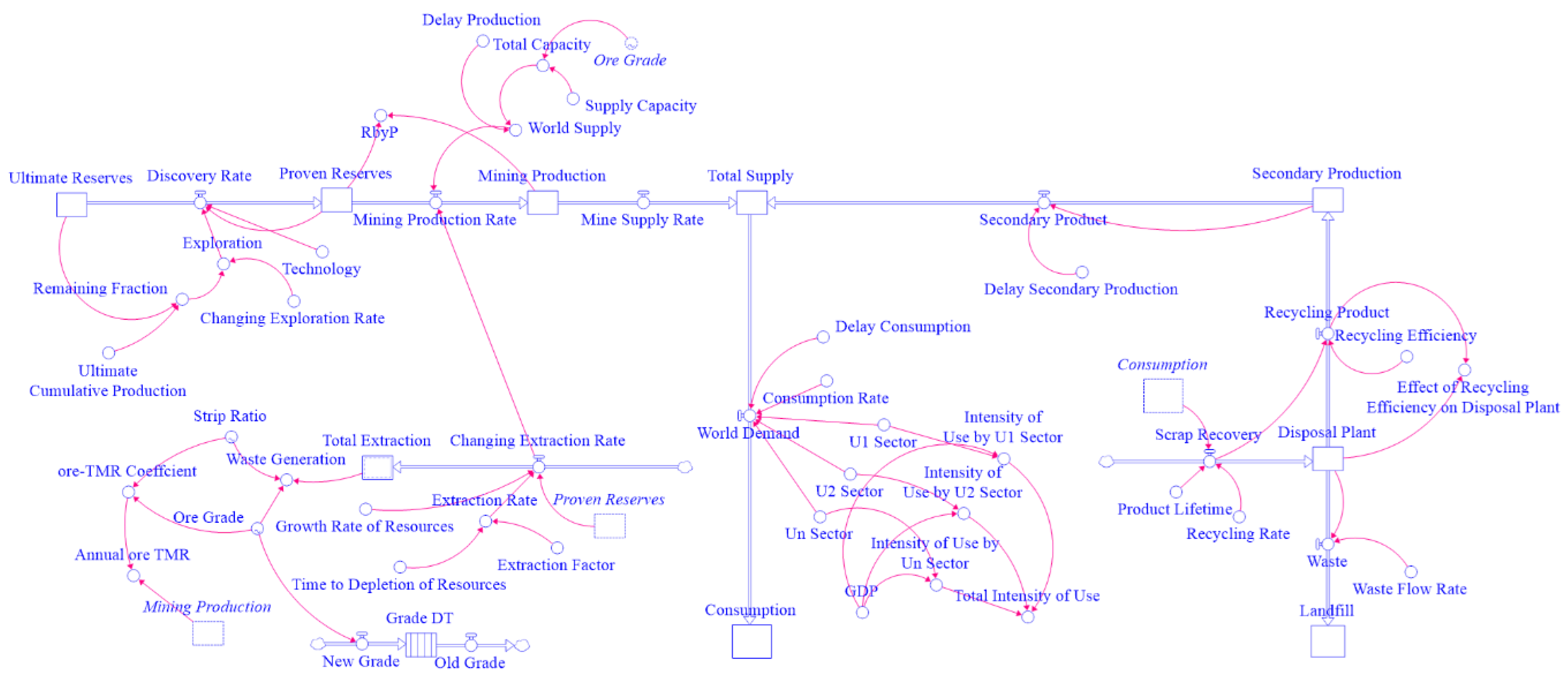
The assumed flow of the metal is shown in Figure 1. Primary reserves of metals are made up of varying sources categorized by geographical location at the country, regional, or global levels. The URRs were estimated by the authors of this study. Metal mining production of either copper or iron depletes these proven reserves, depending on the rates of exploration, technology, discovery, etc. Concurrently, secondary recycling production takes place with scrap recovery from the metal consuming sectors, and the total supply flows to the market stocks as a supply inflow. Metal stockpiles are the mainframe of supply and demand dynamics occurring within the market. The demand for these metals depending on the consuming sectors by application in each industry is shown in Table 1. The degree of the material requirement for consumption varies by the market share of each sector, which can be predicted by their intensity of use. Intensity of use is defined as the amount of metal demanded or consumed per income. Metal recycling is estimated individually based on the retired product lifetime of each sector, with non-recyclable material proceeding to an end-of-life at landfills.
Data obtained were collected primarily from the S&P global database for resource reserve estimates, ore grade, strip ratio, and mining production between 1991–2019 for copper and 2000–2019 for iron. The forecast period covers the long term, from 2020 to 2070. Additional data for metal consumption estimates were collected from the World Bureau of Mining Statistics and the World Steel Association. Other scientific journal papers and reports provided additional estimates of production, recycling, technology, and efficiency rates.
2.1. Resource Estimation
The need for resource definition to reduce physical resource uncertainty is important as it helps in identifying material inputs that are economic and recoverable. Mineral resource availability was modelled on distinguishing resources and reserves according to the modified McKelvey classification [38]. Resources are geological occurrences with an inferred certainty of existence, whereas reserves are resources with a measured and probable certainty of occurrence [38]. Proven reserves are identified, measured, and economically profitable. Cumulative production forms a part of the proven reserves, which increase over time. The limit on the physical availability of economic resources is the URR. A given cut-off ore grade determines the URR. The cut-off grade adjusts to the technological market and geological conditions occurring at the mine site. In this model, the limit of ore grade modelling is assumed at a cut-off grade of 0.2% Cu and 20% Fe, which is a determining factor in limiting future available resources. Grades lower than these predetermined cut-off grades are assumed to be perpetually uneconomic. The reserve base of the producing regions or selected countries for the metal has been used to develop relations between cumulative ore grade and tonnage in previous studies [39]. The relationship fits a log-normal distribution of the metal ore grade and mineral tonnage identical to Lasky’s law for metals such as copper and nickel, and a linear best fit to metals that do not conform to Lasky’s rule, such as gold, iron, or zinc. The global resources regressed are 1.34 Gt Cu and 107.15 Gt Fe [39]. The copper estimates are lower than the USGS 2006 [2,40] of 3.9 Gt Cu, and iron estimates are similar to 170 Gt Fe of USGS 2019 [41], respectively.
2.2. Metal Supply Modelling
2.2.1. Primary Supply
The total extraction of metal mining at a given location (i), either global, regional, or country, is the cumulative production volume of that locality in the current term (t) minus the previous term (t-1). Regional localities were divided into five locations: Africa, Asia Pacific, Europe, Latin America, and North America. At the country level, selected countries were analyzed depending on the country producing that metal (m).
The extraction rate is affected by the growth rate of resources. The extraction factor has a multiplier effect on the extraction. A 0.9 extraction factor was applied to all mine sites [39].
Proven reserve (Rs) tonnage is determined by the difference between newly discovered reserves at a given time (t) of a producer location and those previously discovered. These reserves are affected by the changing discovery rate (DR) over time:
where S is the total metal supply. The discovery rate is inversely proportional to the remaining fraction. Technically, the quantity of proven reserves is equivalent to cumulative production. The latter can never exceed the total reserves of a given region. However, unproven and undiscovered resources can be converted to identified and proven resources at any time, thus changing the size of these reserves, and ultimately be mined economically in the future, even at lower grades.
The ultimate reserves including both cumulative production and proven resources were defined. However, to extract only economically, extractable, and recoverable resources, the URR is defined by the cumulative production in metal ore mining along the production history and at a given economical cut-off grade. These resources were defined by the exploration (E) and technology (T) changes that occur during the lifetime of mining in a given location:
The percentage change in exploration is represented as a function of time (t). The rate of change in exploration was determined by the remaining recoverable resources exploited over time. To stabilize the model, constant κ is applied:
According to [13], the technology rate (r) changes by 0.8% annually. It accounts for all the mining, smelting, and recycling processes that occur over time. In our study, we applied this rate to all the metal models. Even though this rate should be adjusted as a function of time (t), we kept it constant owing to its inelasticity and inertia. We calculated the technological rate as
The changing resource by production ratio (RbyP), which describes the lifetime of commodity (m) in a location (i), was obtained by dividing the proven reserves by the annual production, thereby delineating the resource potential over time.
The remaining recoverable resources reduce over the production lifetime of the mine as the reserves of an ore deposit are depleted. It was defined as the URR minus the cumulative primary mining production:
The supply capacity of the metal ore flow changes over time, assuming that the smelting capacity and total mine capacity are kept constant with a carrying capacity index of 0.9 as the ore grade, and the capacity ore production tonnage flows into production at a given time. Production delay was also assumed, as mine projects do not commence instantly because of their inherent nature. A two-year time delay factor was applied to the model considering that mine projects in the stages of development can take between one and five years to commence [42]:
Mining supply was estimated to determine the cumulative trends for each metal. The logistic curve [43] model was used to forecast by regression, and the cumulative production up to 2070 was estimated for selected countries and regions based on Equation (8):
which can be rewritten as
The annual growth rate of mining production (Pi) was assumed to be constant over time.
2.2.2. Secondary Supply
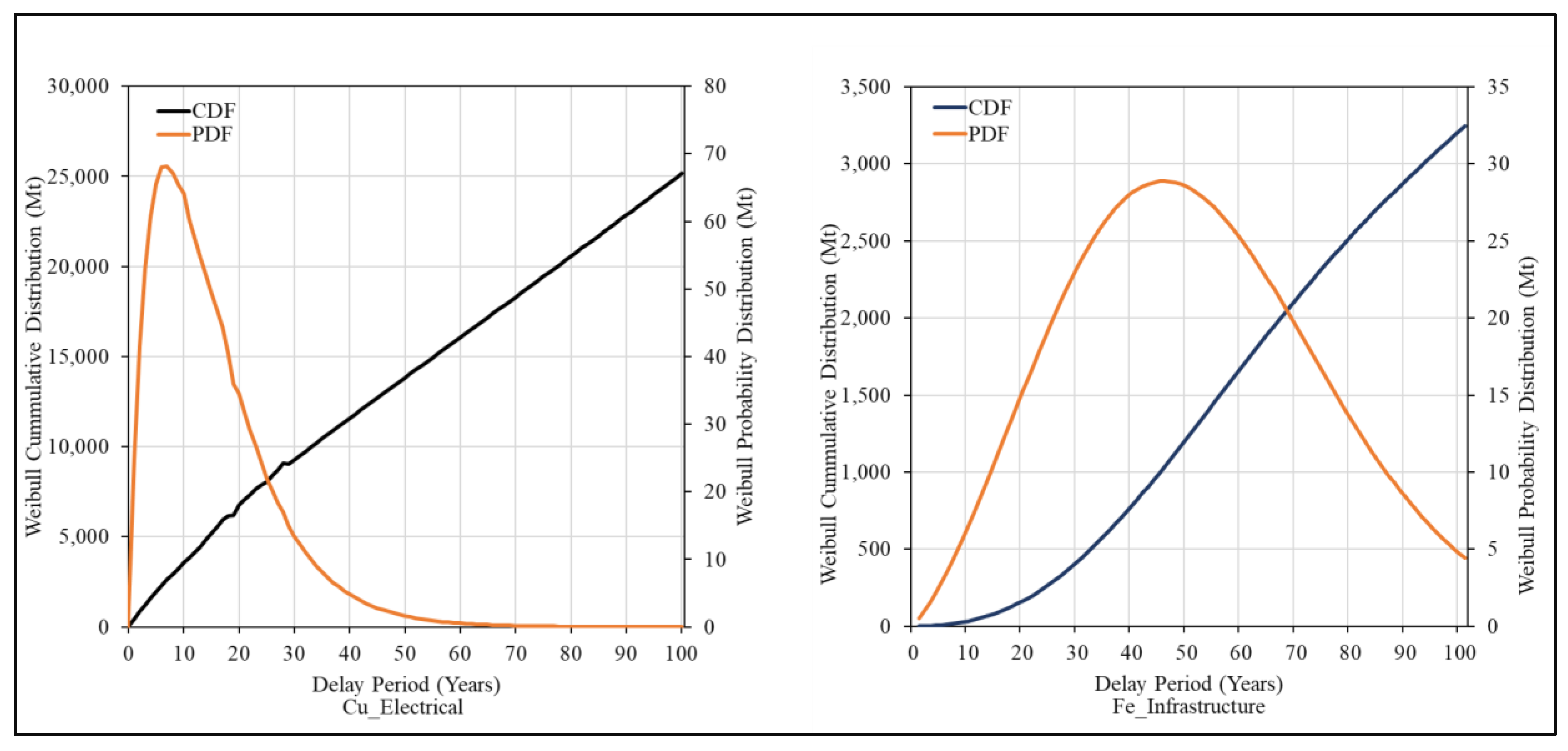
Metal recycling from old scrap is a function of the generation from old scrap and end-of-life recycling rate (EOL-RR). The metal scrap of these resources is generated depending on the product lifetime in the consumption sectors. We estimated this by applying the Weibull distribution, specifically the probability distribution function (PDF). This statistical distribution was adopted in this study to model the metal lifetime of products generally applied in many studies related to stock and obsolete simulations [27,44]. The justification for using the Weibull probability distribution is that it can provide a better goodness of fit than the normal distribution, as it allows factoring in retiring products in their respective sectors that enter their end-of-life to be disposed into landfills. The copper industry includes the electrical, industrial, transport and other minor sectors. The iron industry includes the infrastructure, industrial, and transport sectors. In both of these industries, the share of metal use in each sector is applicable at their market share. The market share was estimated from previous sources [45,46] and is displayed in Table 1. Pr in Equation 9 represents secondary recycling production over time (t). The characteristics of the Weibull (two-parameter Weibull) random variable (x) are characterized by scale parameter (λ), shape parameter (β), and location parameter (α). The scale parameter was predefined in the Excel Solver. The shape parameter (β) represents the lifetime of the metal product. The location parameter in a two-parameter function distribution was insignificant; therefore, it was set to 0. The Weibull distribution is given by
The period of delay (t-tn) in the metal demand creates a periodic lag in the consumption of a metal in the sector. Therefore, the recycling of either copper or iron is simulated as a function of their individual metal demands (Dt) consumed in each sector for usage, with a recycling rate as the Weibull probability distribution (PDF: x, λ, β). The EOL-RR measures the recycling rate as a ratio of the metal in a discarded product separated to obtain recyclates that return to the production processes to the total discarded product inclusive of retired metal [22]. The recycling rates were assumed to be 60% for Cu and 72% for Fe [23].
The annual discard flow amounts, defined as the total quantity of scrap collected from all used products, were calculated for each consumption sector for copper and iron ore. The current scrap recovery rate at the disposal plants is 80% for Cu and 70% for Fe [47,48]. The retiring period was calculated in years, as waste generated at the peak lifetime. The retired lifetime is a part of Equation (9) as follows:
The product delay was measured at the PDF and cumulative distribution function (CDF) intersection point. Figure 2 displays recycling production on the Weibull distribution for the largest consumption sector in the copper and iron markets. Table 1 presents the estimated values for the λ and β parameters used in the Weibull distribution to determine the recycling flows of copper and iron by their respective metal-consuming sectors estimated using Minitab. Furthermore, the residence time to end-of-life was assumed to be constant during the forecast period.
2.2.3. Metal Demand
Current economic growth has led to explosive growth in metal consumption. In addition, the relationship between energy and metal consumption presents a strong interrelationship. Furthermore, the global GDP is expected to grow at an average rate of approximately 3% by 2050 [13,49,50]. In our study, this rate was assumed to remain constant until the year 2070. Van Vuuren et al. expressed metal demand as a function of energy consumption [1]. They outline that about 5–10% of the global primary energy is consumed by metal industries. The link between energy consumption and metal demand is viewed as having a positive linear relationship [51]. Due to the large share of electricity consumption in the total energy demand, it was used as the basis for the interrelationship with the metal consumption of the consuming sectors:
Here, y represents the electricity consumption of a consuming sector u. The electricity consumption was measured as a function of time t, where a and c were constants.
The metal consumption of a consuming sector u was estimated based on the regression equations as a function of electricity consumption in Equation (11). Herewith, metal consumption, Cm, expected to have a demand rate of 3%, was regressed linearly:
Then, metal consumption at the market share of the consuming sector is given by
The carry-forward inventory is the remaining material tonnage left unused by consuming sectors from the previous year. As such, inventory is used as an adjustment to balance the supply and demand of the systems model with changing time. Therefore, a balanced model cannot assume negative conditions. Thus, to measure demand, this carry-forward inventory from the previous year was reduced from the summation of the consuming sectors (Cm,u,t) at the market share (MS):
The trend in intensity of use (IU) is given as a ratio of the metal consumption in sector u by the per capita GDP in a given country or region i. The IU of these metals in their consuming sectors will rise as metal consumption increases and ultimately decline as the sectors mature and demand peaks.
2.2.4. Model Calibration
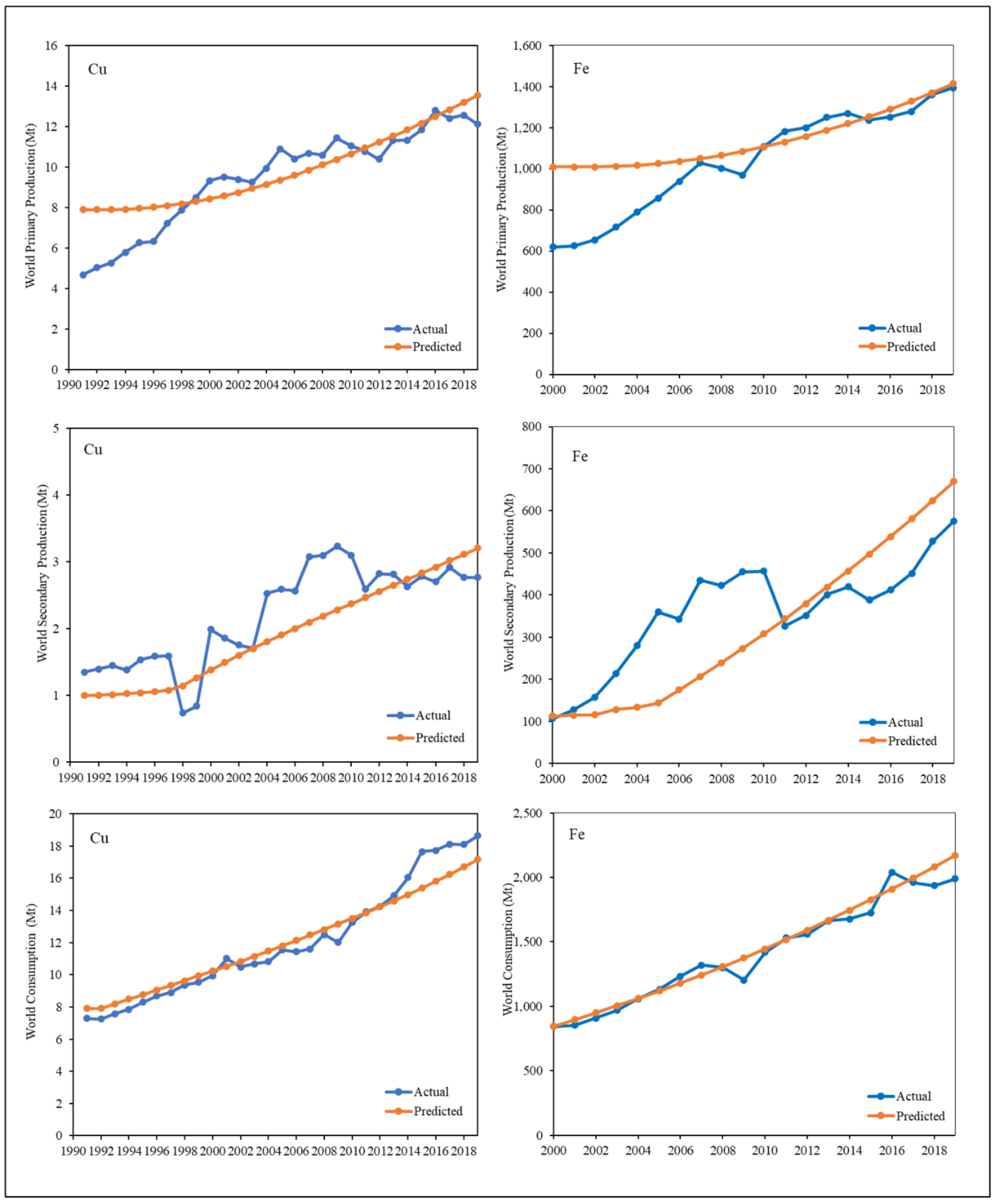
To determine the relevance of the model, it was calibrated by comparative analysis of simulated results from actual historical data through historical matching for copper (1991–2019) and iron (2000–2019) over primary mining production, secondary recycling production, and consumption data. Historical matching is conducted by adjusting a set of model parameters to provide the best possible outcome to stabilize the model before prediction commences. Although historical matching provides past trends, the objective is not to reproduce these trends, but to provide a baseline for the assumption of future long-term trends. Figure 3 displays the historically matched data for copper and iron at the global level.
The root mean square error (RMSE) is the square root of the variance of the residuals that corresponds to the prediction error per square of the given sample population. This criterion depends on the order of magnitude of the observed values, which indicates the absolute fit of the model to the data, that is, how close the observed data points are to the model’s predicted values. The RMSE can be interpreted as the standard deviation of the unexplained variance and has the useful property of being in the same units as the response variable [52]. Lower RMSE values indicate a better fit. The RMSE is a good measure of how accurately the model predicts the response. Table 2 shows the RMSE statistical results for copper and iron at the global level.
3. Results and Discussion
This study confronts the predicament that the physical scarcity of copper and iron resources is unlikely to be constrained over the study period. However, the current supply rates will constrain the primary supply of these metals. Our findings indicate that there would be no major structural changes by 2070 within the copper industry in terms of the main contributor to total supply. However, the secondary supply of iron would become the main source of iron by 2070.
3.1. Copper
3.1.1. Copper Supply and Demand
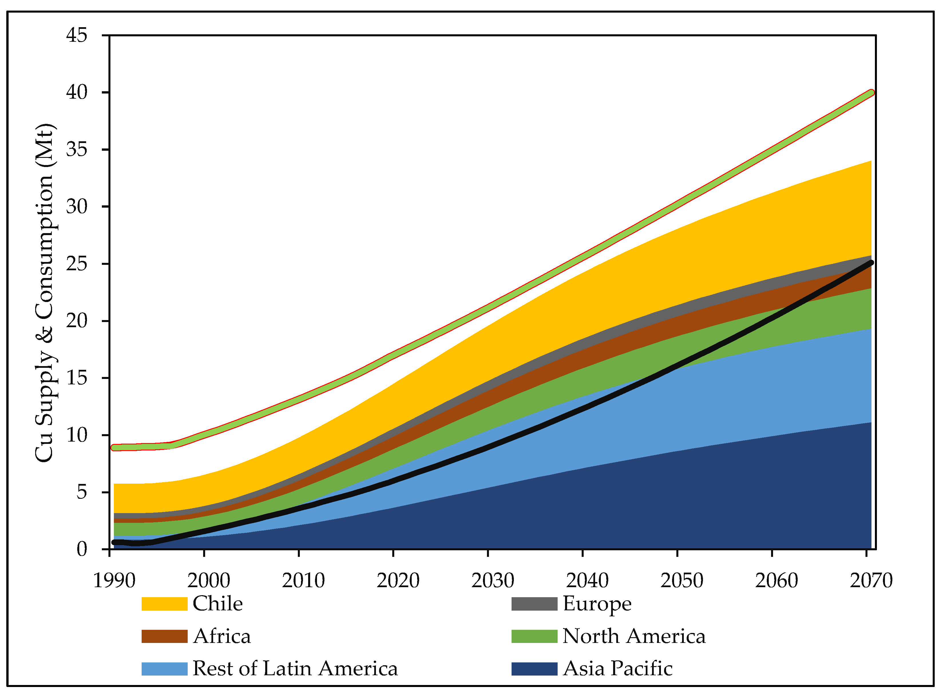
Figure 4 illustrates the trend behavior of primary and secondary supply and the consumption of copper from 1991 to 2070. From this figure, the base scenario assumes that primary copper reserves are not sufficient to support the future copper availability for the increasing demand by 2070; thus, recycling as a secondary source of copper production is necessary to sustain future supply. Total supply will increase from 8.89 Mt in 1991 to 39.9 Mt in 2070. The primary copper production will remain the main source of copper in 2070 with production volume increase of 26.8 Mt (2070) from 7.89 Mt (1991). Latin America presents itself as the main producer of copper as shown in Figure 4, with the production volume doubling from 7.5 Mt (2020) to 16.4 Mt (2070). Furthermore, metal mining in the Asia-Pacific region is expected to triple from 3.7 Mt (2020) to 11.1 Mt (2070) at a 1.4% growth rate. The scale of mining in the European region would remain significantly small. If we look at countries instead of region, Chile continues to play a significant role in copper supply, given the large Chilean scale in production (Figure 4). Furthermore, we observe peaking in primary production as the production rate decreases to stabilize at around 2% by 2060.
Meanwhile, the current EOL-RR at 60% is expected to rise steadily until 2070 to sustain the total copper supply. The secondary supply increases from 1 Mt (1991) to 13.1 Mt (2070), accounting for 33% of the total copper contribution by 2070. This trend is driven by the estimated consumption which will grow from 7.9 Mt to 39.6 Mt between 1991 and 2070 at an average growth rate of 0.43%. The electrical (E), industrial (I), transport (T), and other (O) applications are sectors of the copper industry at 26%, 19%, 3%, and 42%, respectively, at their market shares [44,45]. This scenario was consistent with the base model proposed by [13]. In their analysis, the primary copper supply was the main source of the total supply till 2070 but began to decelerate from 2090. The consumption trends in millions of tons of these applications regressed as follows:
CCu,E,MS,t = 0.222t − 306,855 (R2 = 0.958)
CCu,I,MS,t = 0.239t − 296,866 (R2 = 0.958)
CCu,T,MS,t = 7.686t − 530,326 (R2 = 0.912)
CCu,O,MS,t = 4.926t + 2,851,125 (R2 = 0.948)
CCu,I,MS,t = 0.239t − 296,866 (R2 = 0.958)
CCu,T,MS,t = 7.686t − 530,326 (R2 = 0.912)
CCu,O,MS,t = 4.926t + 2,851,125 (R2 = 0.948)
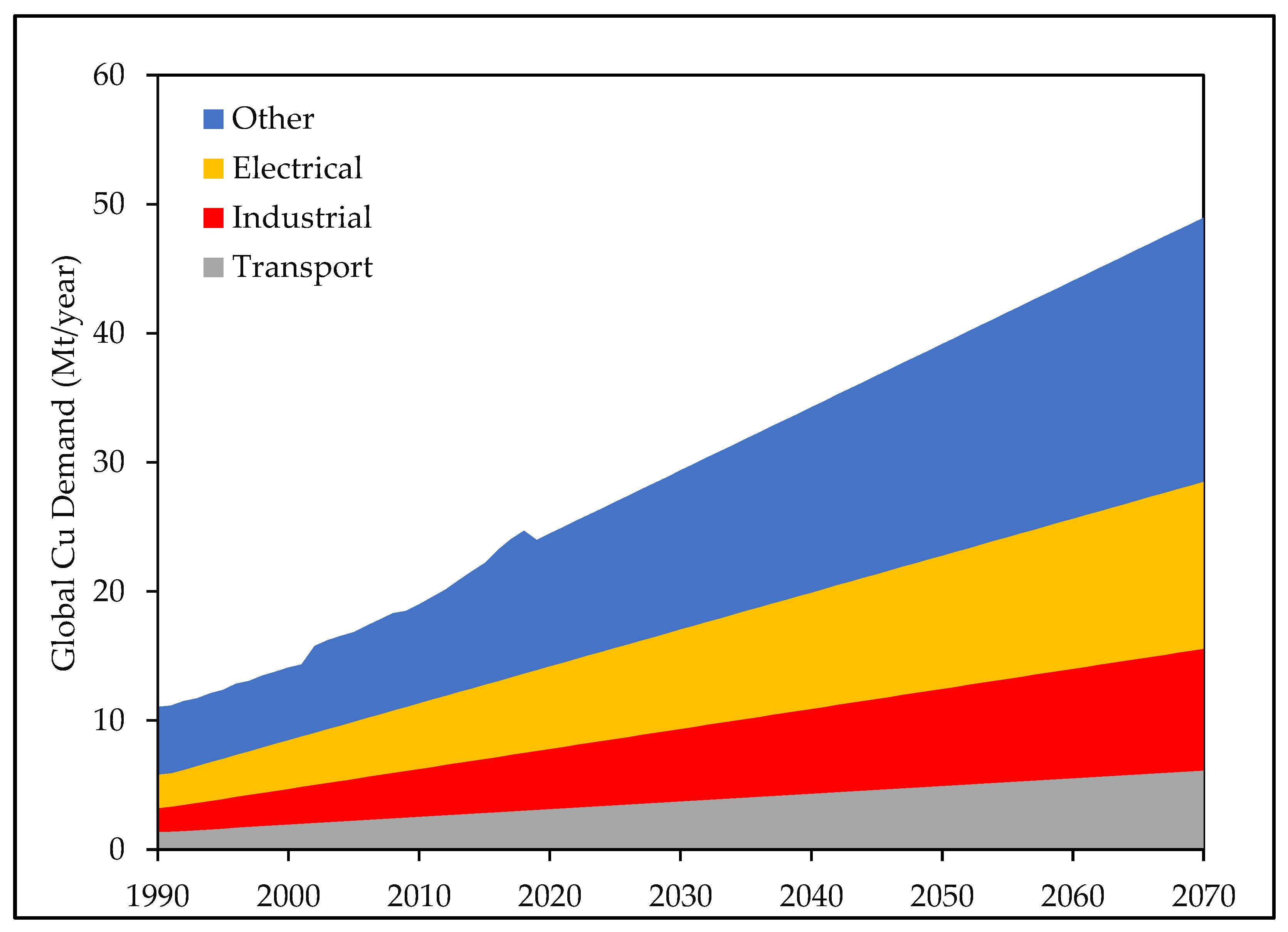
Figure 5 shows that the copper sectorial demand trends demonstrate a monotonic increase until 2070. The sectorial demand of the sectors accelerates at varying demand rates, with the total demand increasing by almost five times in 2070 to 48.8 Mt/year compared to 1991. The increase is slightly lower than that reported by [2,14], which ranged from 50 to 50–80 Mt/year in 2070. Moreover, the estimates vary by analytical methodology. The electrical sector has the largest demand by market share increasing from 5.2 Mt/year to 20.4 Mt/year over the study period followed by the industrial and transport sectors and to a lesser extent the agglomeration of minor shares.
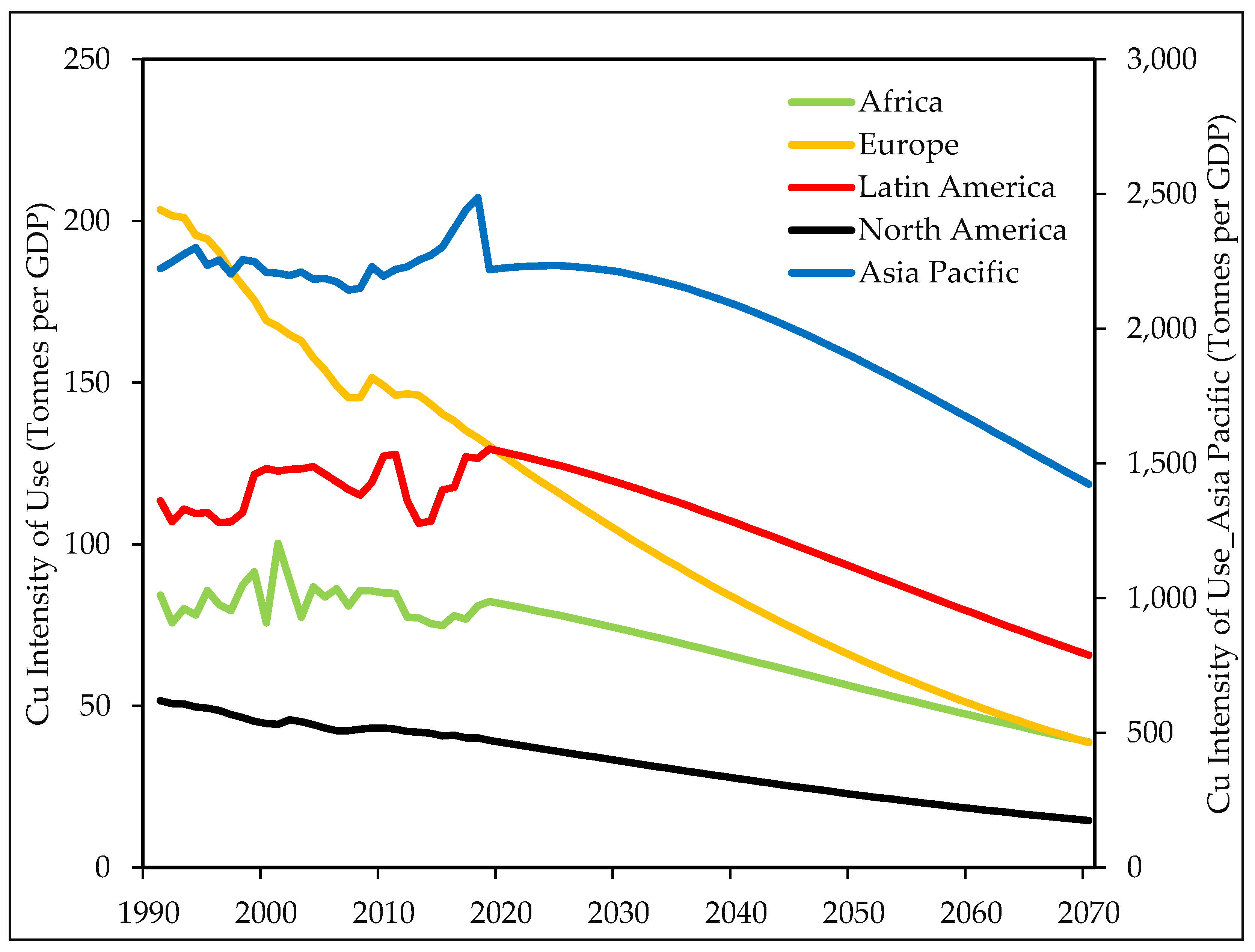
The IU in the transport, industrial, electrical, and other sectors that inherently reflect future demand projections for copper show monotonic increases over time, as shown in Figure S1. The major demand for copper is sourced from other sectors, which is a summation of various minor sectors, followed by the electrical, industrial, and transport sectors. The Asia-Pacific trend displays a steeper IU pattern in the electrical sector, which decelerates quickly as material consumption reduces in the region but remains high in the comparative sectors. Figure 6 shows the total intensity of copper use in each region. Asia-Pacific, Europe, Latin America, Africa, and North America show the order of increasing IU from highest to lowest. The trend in IU in Europe shows a rapid decline from the beginning of the study period. By 2040, the IU of all the regions will decline as the copper sector reaches maturity through economic development. By application share, Africa’s IU in the transport sector declines to 3.2 tons per GDP by 2070 and Latin America’s IU falls to 4.1 tons per GDP over the same period. In the industrial sector, by 2070, the IU of use will remain above 5 tons per GDP. Owing to the rapid development of electrical applications in the Asia-Pacific region, the resource IU indicates a drop as it has been on an accelerating decline since the early 2000s and falls below Latin America around 2020. North America indicates a relatively low material intensity for consumption in the electrical sector (Figure S1).
3.1.2. Copper Sensitivity Analysis
Regarding secondary consumption, two major factors are important for future scrap availability: recycling efficiency and EOL-RR. Product lifetime and in-use stock from the consuming sectors are intrinsically linked to the recycling rate. The parametric value of the recycling rate was 58.5%. Previous literature assumes an EOL-RR between 45–80% varying at the global, regional, or country level [11,19,22,27,50]. Assuming a 75% increase in EOL-RR improves it by 2070 to 42 Mt, such that recycling processes become the main copper source of supply. At 75% sensitivity, the simulated resource efficiency would be equivalent. These two factors show that copper recycling could still be improved to increase recycling production, ultimately reducing environmental consequences.
3.1.3. Sustainable Use of Copper
The global production of copper is concentrated in Latin American regions, specifically Chile. This region has become a hotspot for copper production owing to the resource governance, ore grade, and large copper reserves in the area. The ultimate resources with a maximum cut-off grade of 0.2% Cu are not a concern for the scarcity of the resource by 2070.
The ability to safeguard the availability of copper for future generations depends on the end-of-life recycling rate and recycling efficiency. A recycling rate of at least 75% is required to achieve copper sustainability in the future. While past studies estimated the current recycling efficiency at 84% [11,19,20], we applied a recycling efficiency of 66%. With the rapid decline in copper ore grade, recovery becomes more difficult over time as the cost of returns increases; hence, adjusting these efficiencies for practical scenarios of copper use will provide a better understanding of resource stakeholders. The application of a specific product lifetime for copper improved the model by underpinning the copper rate of demand.
3.2. Iron
3.2.1. Iron Supply and Demand
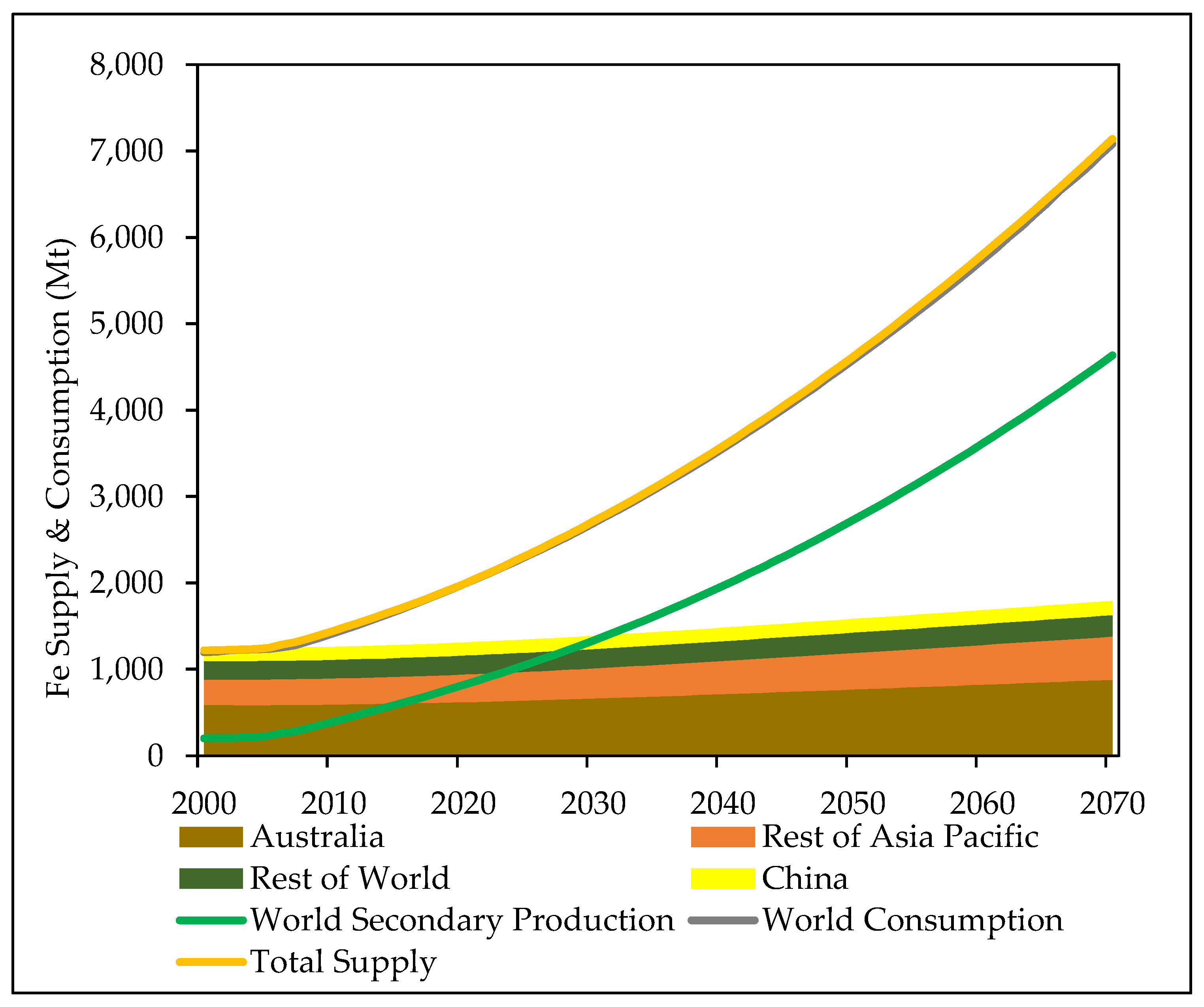
The global model is iteratively calculated with the adjustment parameter set to balance the model and minimize the error from the actual value by historical matching. In this study, primary mining production refers to the summation of iron production from direct reduced iron (DRI) and electric arc furnace processes (EAF). This assumption is preferred to reduce the complexity of the material balance in modeling the iron ore. In addition, the amount of iron ore sent into the DRI and EAF is equivalent to the iron ore mining production. Figure 7 illustrates the base scenario trend between total iron supply and consumption by 2070. The simulation scenario in the base case shows that the iron supply will increase by three-fold of the current level, from 1220 Mt to 7190 Mt. This figure shows that primary iron ore production is the main source of iron supply. Primary production is projected to increase from 1420 Mt in 2020 to 2555 Mt in 2070. However, in 2033, secondary production processes with quantities of 1510 Mt surpass conventional mining, increasing its iron share proportion to 66% (by 2070) to sustain the demand for crude steel consumption by 2070 with 4634 Mt. World consumption increases from 1019 Mt in 2000 to 7140 Mt in 2070. In addition, there will be intermittent periods of excess supply between 2030 and 2070. The numerical crude steel consumption was relatively consistent with that in existing literature. In our findings, in 2010, crude steel consumption was 1458 Mt, compared to 1433 Mt [53] and 1417 Mt [16]. In 2050, crude steel consumption is expected to reach 3370 Mt compared to 3291 Mt predicted by [16] in their high-demand case. The rate of consumption will increase from 0.3% in 2020 to 0.75% in 2070, as illustrated in Figure 7.
The Asia-Pacific region has the largest cumulative share in iron ore supply of >80%, which increases from 1047 Mt in 2000 to 1573 Mt in 2070. Australia is the top iron ore producing country, accounting for approximately 50% of the total share of production. Australian production would increase from 586 Mt in 2000 to 881 Mt in 2070. Around 2010, Australia experienced large-scale iron ore production to cater to increasing demand in China. While China is a large consumer of iron for steel production, its national production remains low because of the low ore grades found in the country. Primary production changes from 146 Mt to 161 Mt over the study period. The old scrap supply could reduce up to 80% of the iron ore required for steel production in China by 2050 [16,54,55].
Classification of iron manufacturing demand was based on previous studies [42,43]. According to these sources, the iron usage percentage share (MS), 52% in construction (C), 34% in industrial (I), and 14% in the transportation (T) industries [45], is estimated using Equation (13). The consumption trends of these applications were expressed in million tons, as follows:
CFe,C,MS,t = 6.235t + 6.565 × 10⁸ (R2 = 0.620)
CFe,I,MS,t = 0.30t − 3.278 × 10⁷ (R2 = 1.000)
CFe,T,MS,t = 828.08t − 1.182 × 10⁷ (R2 = 0.634)
CFe,I,MS,t = 0.30t − 3.278 × 10⁷ (R2 = 1.000)
CFe,T,MS,t = 828.08t − 1.182 × 10⁷ (R2 = 0.634)
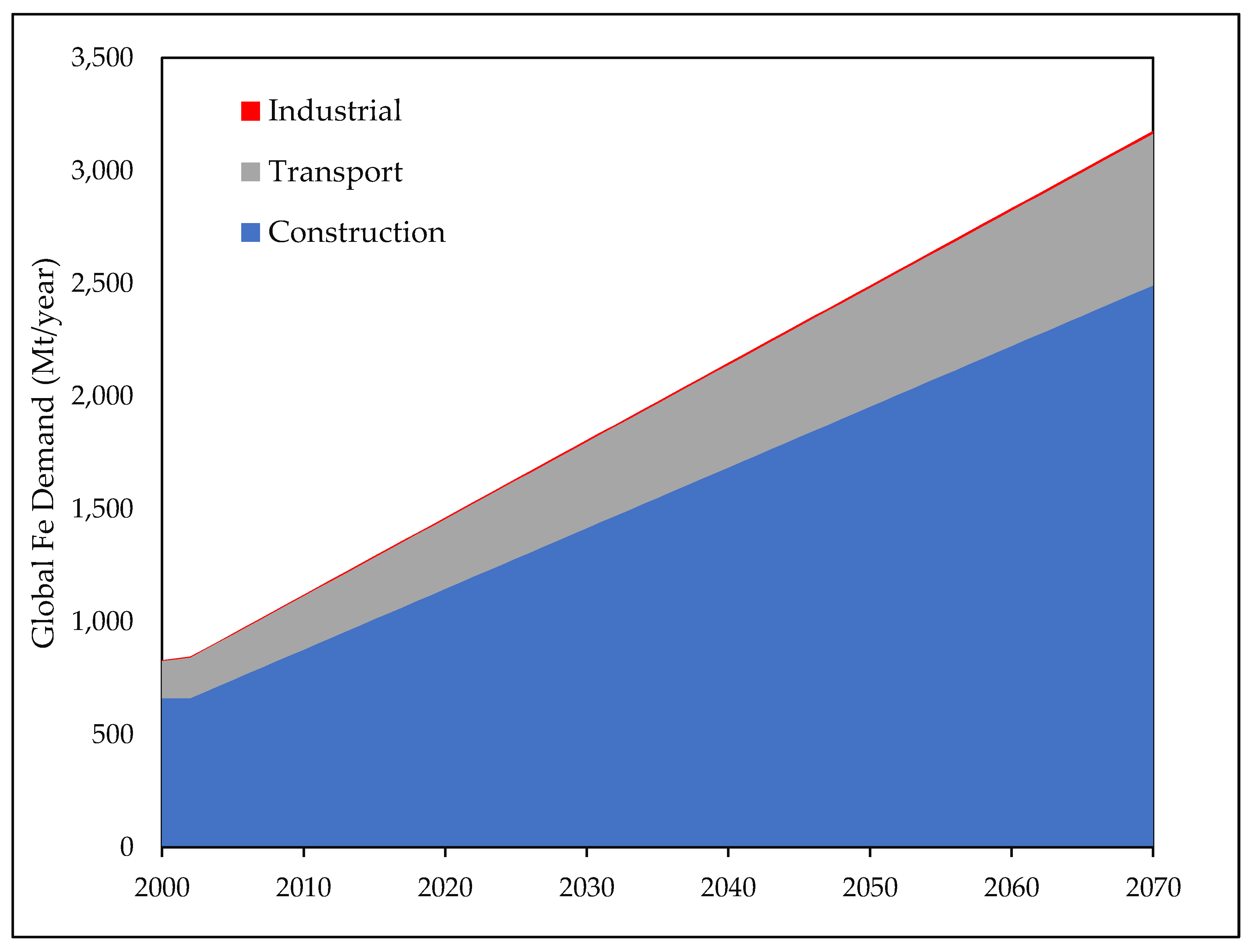
Figure 8 illustrates the iron demand trends till 2070 by sectorial market share. The major iron demand is utilized in the construction sector, followed by the transport and industrial sectors. This large share of construction is largely accounted for by China’s large-scale consumption to support its national industrial growth for development, which has been a leading potential market for iron since the early 2000s. The total demand for iron steel has grown to more than 3 Gt of Fe by 2070. This trend is supported by literature [17,54,55,56,57].
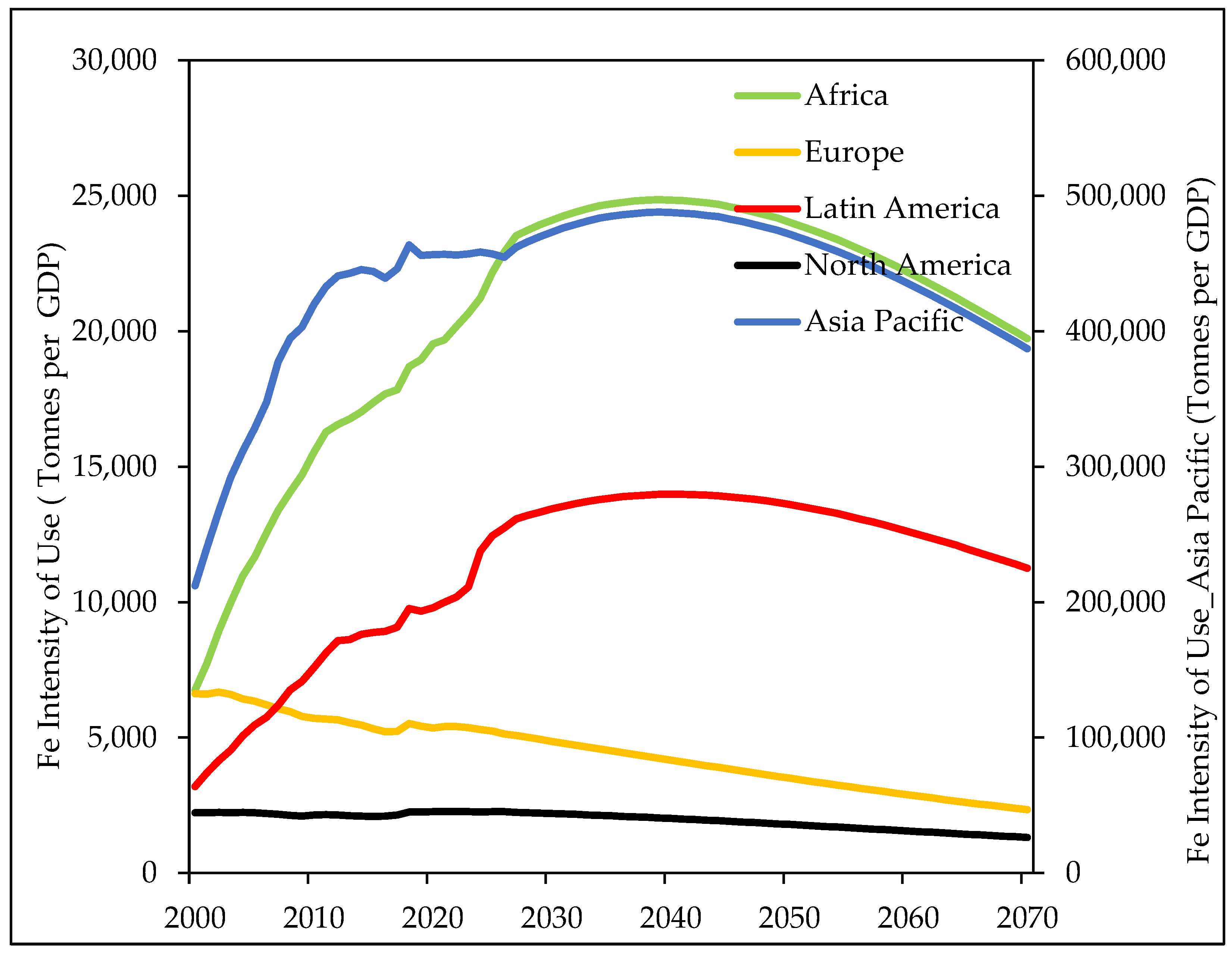
Resource use per GDP was simulated based on the demand trends (Figure S2) for each sector. Similar to copper, the future intensity of use exemplifies monotonic increases over time, before declining in 2070. However, the Asia-Pacific region has a steeper deceleration in the industrial sector. In the construction sector, the Asia-Pacific and African regions have similar intensity of use of future patterns with a significantly large gap between the two trajectories as the African trend trails behind. In addition, Figure 9 shows that the Asia–Pacific region has the largest IU trajectory in the long term. The North American region, which consists of advanced economies such as the United States and Canada, requires minimal resource consumption of approximately 2500 tons per GDP, as their economic focus would shift to services. Africa’s developing countries are expected to advance rapidly before peaking before 2050 to become more advanced than Latin America.
3.2.2. Iron Sensitivity Analysis
Recycling efficiency and EOL-RR were estimated to be 43.7% and 33%, respectively. Recycling efficiency is consistent with various sources [22]. The model-based recycling rate is pessimistic compared to previous studies [16,22,57,58] because it is based on the assumed product lifetime duration function. According to Oda et al, a recycling rate of 85% could lead to an overestimation of the future scrap availability [16]. At the global scale, 70% of EOL-RR is applied [15,16]. Recycling efficiency significantly influences the degree of secondary production compared to recycling rate. Raising or lowering recycling efficiency has a decelerating effect on scrap recovery. The recycling rate at current levels is optimized, and the recycling efficiency is approximately 60%. This is because, at every steel plant, a recycling plant also preferentially exists, and all steel production consumes scrap, resulting in a high level of recycling from iron to steel with very limited room for improvement and material loss [54]. To increase the recycling efficiency by 100%, the recycling rate should be equal to the simulated secondary production level. Currently, the ratio of recycling efficiency to recycling rate is 0.6. However, lowering the recycling efficiency to between 25–75% would result in a lower recycling rate.
3.2.3. Sustainable Use of Iron
Iron ore primary production would be surpassed by secondary recycling by the mid-2030s to become the main source of resource supply by 2070. Even though iron ore resource/reserve size is abundant and requires ample exploration for new discoveries, the resource industry continues to improve the recycling industry for steel production [54] and would raise the recycling efficiency to the recycling rate ratio. This industrial practice will ensure sustainability, and future availability should rise at increasingly exponential rates.
The majority of global iron mine production activities occur in the Asia-Pacific region, with Australia being one of the top producing countries. For consumer countries, this provides a geographical advantage to accessing the iron markets, especially fast-increasing economies such as China.
4. Conclusions
A sustainable future through sourcing and consumption of resources is at the forefront of comprehensively understanding the present value of these resources. The present trends in global resource extraction are steeply rising, with no significant signs of slowing down, leading to concerns about the sustainability of resource supply in the future [30,31]. No generally accepted global level quantitative resource scenarios exemplifying resource extraction and use exist at present, which can be considered to be a huge gap in addressing resource challenges [30,31].
Whether these resources are “finite” or the impact of mining puts pressure on the environment; both allow for a sustainability model. While the existing literature denotes varying future projections of the future metal supply, they provide valuable hypotheses with regard to resource accountability and management [7,37]. Therefore, this study aimed to develop a systems framework in which metals could be quantitatively measured in the long term for future resource availability as a measure of supply risk. Critical issues of physical scarcity and sustainability were addressed.
From this study, it was found that the ultimate recoverable reserves of copper and iron are unlikely to constrain long-term resource supply. However, the annual production rate and technological advancement of mining will influence the trajectory of resource supply. The future demand and consumption of copper and iron are expected to increase from their current levels due to metal application. As the mining supply rises to support the consumption sectors, mining production will eventually peak. This would require an increase in secondary production to support the availability of resources. Primary copper production is expected to remain the main source of copper, while secondary iron production will become the main source of iron by 2070.
On the demand side, the consumption sectors of these metals as a function of the per capita GDP are the driving factors of material flow in the systems. Their IU was determined to delineate the share of material consumption per sectorial use.
The modeling framework presented in the study provides a foundational basis for a quantitative framework that could be extended to a multivariable study of environmental footprints, such as carbon emissions and energy consumption and their associated roles that could likely lead to restrictions in future resource supply. Furthermore, as a limitation to the model to improve this study, future analysis accounting for metal substitution and other factors (economic, social, or economic) in the systems framework would provide a detailed scenario of systems interaction that would enable policy planning for a sustainable environment.
Finally, the application of the mining histories of metals convey an understanding of the material balance in metal supply by providing resource stakeholders with provisional forecast estimates of future quantities. However, the underlying issue of linking material extraction and consumption to the environment requires extensive debate on mining sustainability. As such, these long-term trends intend to create a balance between the resources we need today and those required in the future.
Supplementary Materials
The following supporting information can be downloaded at: https://0-www-mdpi-com.brum.beds.ac.uk/article/10.3390/resources11040037/s1, Figure S1: Copper Intensity of Use by sectorial share; Figure S2: Iron Intensity of Use by sectorial share.
Author Contributions
Conceptualization, L.S.T. and T.A.; methodology, L.S.T. and T.A; software, L.S.T. and T.A.; validation, L.S.T. and T.A; formal analysis, L.S.T.; investigation, L.S.T.; resources, T.A.; data curation, L.S.T.; writing—original draft preparation, L.S.T.; writing—review and editing, L.S.T.; visualization, L.S.T. and T.A; supervision, T.A.; project administration, L.S.T. and T.A.; funding acquisition, T.A. All authors have read and agreed to the published version of the manuscript.
Funding
This research was funded by the ‘New Frontier Leaders for Rare Metals and Resources’ graduate program of Akita University.
Institutional Review Board Statement
Not applicable.
Informed Consent Statement
Not applicable.
Data Availability Statement
The data used in this article are freely available.
Acknowledgments
This research was supported by Akita University.
Conflicts of Interest
The authors declare that they have no conflict of interest. The funders had no role in the design of the study; in the collection, analyses, or interpretation of data; in the writing of the manuscript, or in the decision to publish the results.
References
- van Vuuren, D.P.; Strengers, B.J.; De Vries, H.J.M. Long term perspectives on world metal use-a-systems-dynamics model. Resour. Pol. 1999, 25, 239–255. [Google Scholar] [CrossRef]
- Tokimatsu, K.; Murakami, S.; Adachi, T.; Ii, R.; Yasuoka, R.; Nishio, M. Long-term demand and supply of non-ferrous mineral resources by a mineral balance model. Miner. Econ. 2017, 30, 109–206. [Google Scholar] [CrossRef]
- Meadows, D.H.; Meadows, D.L.; Randers, J.; Behrens, W.W. The Limits to Growth; Universe Books: New York, NY, USA, 1972. [Google Scholar]
- Meadows, D.; Randers, J.; Meadows, D. A Synopsis: Limits to Growth: The 30-Year Update; Chelsea Green Publishing Company: White River Junction, VT, USA, 2004; Available online: https://donellameadows.org/archives/asynopsis-limits-to-growth-the-30-year-update/ (accessed on 3 March 2021).
- Norgate, T.E.; Rankin, W.J. Life cycle assessment of copper and nickel production. In Proceedings of the Minprex 2000, International Conference on Mineral Processing and Extractive Metallurgy, Melbourne, (Victoria), Australia, 11–13 September 2000; Available online: https://www.ausimm.com/publications/conference-proceedings/minprex-2000/life-cycle-assessment-of-copper-and-nickel-production/ (accessed on 24 May 2021).
- Crowson, P.C.F. Mineral reserves and future mineral availability. Miner. Econ. 2011, 24, 1–6. [Google Scholar] [CrossRef]
- Northey, S.; Mohr, S.; Mudd, G.M.; Weng, Z.; Giurco, D. Modelling future copper grade decline based on a detailed assessment of copper resources and mining. Resour. Conser. Recyl. 2014, 83, 190–201. [Google Scholar] [CrossRef]
- Calvo, G.; Mudd, G.; Valero, A.; Valero, A. Decreasing ore grades in global metallic mining: A Theoretical Issue or a Global Reality? Resources 2016, 5, 36. [Google Scholar] [CrossRef] [Green Version]
- Meinert, L.D.; Robinson, G.R.; Nassar, N.T. Mineral Resources: Reserves, Peak Production and the Future. Resources 2016, 5, 14. [Google Scholar] [CrossRef]
- Pagani, M.; Bardi, U. Peak Minerals (2007). In The Oil Drum: Europe; ODAC Newsletter: UK, 2016. [Google Scholar] [CrossRef]
- Henkens, M.L.C.M.; Worrell, E. Reviewing the availability of copper and nickel for future generations. The balance between production growth, sustainability and recycling rates. J. Clean. Prod. 2020, 264, 121460. [Google Scholar] [CrossRef]
- Roper, L.D. World Mineral Reserves, 2009. Website with Hubbert’s Type Variant of Resource Assessment. Available online: http://www.roperld.com/science/minerals/Reserves.htm (accessed on 1 September 2021).
- Adachi, T.; Mogi, G.; Yamatomi, J.; Murakami, S.; Nakayama, T. Modeling global supply-demand structure of mineral resources- long term simulation of copper supply. J. MMIJ 2001, 117, 931–939. (In Japanese) [Google Scholar] [CrossRef] [Green Version]
- Ayres, R.U.; Ayres, L.W.; Rade, I. The Life Cycle of Copper, Its Coproducts and Byproducts; Kluwer Academic Publishers: Dordrecht, The Netherlands, 2003. [Google Scholar]
- Neelis, M.L.; Patel, M.K. Long-Term Production, Energy, Consumption, and CO2 Emission Scenarios for the Worldwide Iron and Steel Industry; Utrecht University: Utrecht, The Netherlands, 2006; Available online: https://dspace.library.uu.nl/handle/1874/21823 (accessed on 20 May 2021).
- Oda, J.; Akimoto, K.; Tomoda, T. Long-term global availability of steel scrap. Resour. Conserv. Recycl. 2013, 81, 81–91. [Google Scholar] [CrossRef]
- Müller, D.B.; Wang, T.; Duval, B. Patterns of iron use in societal evolution. Environ. Sci. Technol. 2011, 45, 182–188. [Google Scholar] [CrossRef]
- Cullen, J.M.; Allwood, J.M.; Bambach, M.D. Mapping the global flow of steel: From steelmaking to end-use goods. Environ. Sci. Technol. 2012, 46, 13048–13055. [Google Scholar] [CrossRef] [PubMed]
- Glöser, S.; Soulier, M.; Espinoza, L.T.; Faulstich, M. Using dynamic stock & flow models for global and regional material and substance flow analysis in the field of industrial ecology: The Example of a Global Copper Flow Model. In Proceedings of the 31st International Conference of the Systems Dynamics Society, Cambridge, MA, USA, 21–25 July 2013. [Google Scholar]
- Glöser, S.; Soulier, M.; Espinoza, L.A.T. Dynamic analysis of global copper flows. Global stocks, postconsumer material flows, recycling indicators, and uncertainty evaluation. Environ. Sci. Technol. 2013, 47, 6564–6572. [Google Scholar] [CrossRef] [PubMed]
- Laherrere, J. Copper Peak. Oil Drum Eur. 2010, 6307, 1–27. Available online: http://europe.theoildrum.com/node/6307 (accessed on 2 August 2021).
- UNEP. Decoupling Natural Resource Use and Environmental Impact from Economic Growth, A Report of the Working Group on Decoupling to the International Resource Panel; Fischer-Kowalski, M., Swilling, M., von Weizsäcker, E.U., Ren, Y., Moriguchi, Y., Crane, W., Krausmann, F., Eisenmenger, N., Giljum, S., Hennicke, P., Eds.; International Resource Panel: Nairobi, Kenya, 2011; Available online: https://www.resourcepanel.org/reports/decoupling-natural-resource-use-and-environmental-impacts-economic-growth (accessed on 30 November 2021).
- UNEP. Recycling Rates of Metals-A status Report, A Report of the Working Group on the Global Material Flows to the International Resource Panel; Graedel, T.E., Allwood, J., Birat, J.-P., Reck, B.K., Sibley, S.F., Sonnemann, G., Buchert, M., Hagelüken, C., Eds.; International Resource Panel: Nairobi, Kenya, 2011; Available online: https://www.resourcepanel.org/reports/recycling-rates-metals (accessed on 30 October 2021).
- UNEP. Global Material Flows and Resource Productivity: An assessment study of the UNEP International Resource Panel; Schandl, H., Fischer-Kowalski, M., West, J., Giljum, S., Dittrich, M., Eisenmenger, N., Geschke, A., Lieber, M., Wieland, H.P., Schaffartzik, A., Eds.; United Nations Environment Programme: Paris, France, 2016. [Google Scholar]
- UNEP. Global Resources Outlook 2019: Natural Resources for the Future We Want; Oberlle, B., Bringezu, S., Hatfeld-Dodds, S., Hellweg, S., Schandl, H., Clement, J., Cabernard, L., Che, N., Chen, D., Droz-Georget, H., et al., Eds.; International Resource Panel United Nations Environment Programme: Nairobi, Kenya, 2019. [Google Scholar]
- Teseletso, L.S.; Adachi, T. Future availability of mineral reources: Ultimate Reserves and Total Material Requirement. Miner. Econ. 2021, 1–18. [Google Scholar] [CrossRef]
- Tilton, J.E. Exhaustible resources and sustainable development: Two Different Paradigms. Resour. Pol. 1996, 22, 91–97. [Google Scholar] [CrossRef]
- Humphreys, D. Long-run availability of mineral commodities. Miner. Econ. 2013, 26, 1–11. [Google Scholar] [CrossRef]
- Mudd, G.; Weng, Z.; Jowitt, S. A detailed assessment of global Cu resource trends and endowments. Econ. Geo. 2013, 108, 1163–1183. [Google Scholar] [CrossRef]
- Bringezu, S.; Moriguchi, Y. Material Flow Analysis. In A Handbook of Industrial Ecology; Ayres, R.U., Ayres, L.W., Eds.; Edward Elgar Publishing Limited: Cheltenham, UK, 2002; pp. 79–90. [Google Scholar]
- Spatari, S.; Bertram, M.; Gordon, R.; Henderson, K.; Graedel, T. Twentieth century copper stocks and flows in North America: A Dynamic Analysis. Ecol. Econ. 2005, 37–51. [Google Scholar] [CrossRef]
- Fischer-Kowalski, M.; Krausmann, F.; Giljum, S.; Lutter, S.; Mayer, A.; Bringezu, S.; Moriguchi, Y.; Schütz, H.; Schandl, H.; Weisz, H. Methodology and indicators of economy-wide material flow accounting—State of the art and reliability across sources. Ind. Econ. 2011, 15, 855–876. [Google Scholar] [CrossRef]
- European Communities. Economy-Wide Material Flow Accounts and Derived Indicators: A Methodological Guide; Office for Official Publications of the European Communities: Luxembourg, 2001. [Google Scholar]
- van der Voet, E.; van Oers, L.; Moll, S.; Schütz, H.; Bringezu, S.; de Bruyn, S.; Sevenster, M.; Warringa, G. Policy Review on Decoupling: Development of Indicators to Assess Decoupling of Economic Development from Environmental Pressure in the EU-25 and AC-3 Countries; Commissioned by European Commission, DG Environment, to support the Thematic Strategy for the Sustainable Use of Natural Resources; European Community: RA Leiden, The Netherlands, 2005. [Google Scholar]
- van der Voet, E.; van Oers, L.; Verboon, M.; Kuipers, K. Environmental Implications of Future demand scenarios of metals: Methodology and applications to the case of seven major metals. J. Ind. Ecol. 2018, 23, 141–155. [Google Scholar] [CrossRef] [Green Version]
- Haraldsson, R.; Sverdrup, H.U. On aspects of system analysis and dynamics work-flow. In Proceedings of the System Dynamics Society, 2005 International Conference on System Dynamics 1–10, Boston, MA, USA, 17–21 July 2005; Available online: https://proceedings.systemdynamics.org/2005/proceed/index.html (accessed on 20 May 2021).
- Sverdrup, H.U.; Oladsdottir, A.H.; Ragnardottir, K.V. On modelling the global copper, zinc and lead supply, using a system dynamics model. Resour. Conserv. Recycl. X 2019, 4, 100007. [Google Scholar] [CrossRef]
- Sverdrup, H.U.; Ragnardottir, K.V. On modelling the global copper mining rates, market supply, copper price and the end of copper reserves. Resour. Conserv. Recycl. 2014, 87, 158–174. [Google Scholar] [CrossRef]
- USGS. 1995 National Assessment of United States Oil and Gas Resources; US Geological Survey Circular; US Geological Survey; The INGAA Foundation: Fairfax, VA, USA, 1995.
- Tilton, J.E.; Lagos, G. Assessing the long-run availability of copper. Resour. Pol. 2007, 32, 19–23. [Google Scholar] [CrossRef]
- USGS. Mineral Commodities Summaries 2020 Iron, 88–89, January 2020; US Geological Survey: Reston, VA, USA, 2020. Available online: https://pubs.usgs.gov/fs/fs024-98/ (accessed on 20 May 2020).
- AusIMM. Cost Estimation Handbook, 2nd ed.; Monograph 27; The Australian Institute of Mining of Mining and Metallurgy: Carlton, Australia, 2012. [Google Scholar]
- Höök, M.; Junchen, L.; Oba, N.; Snowden, S. Descriptive and predictive growth curves in energy system analysis. Nat. Resour. Res. 2012, 20, 103–116. [Google Scholar] [CrossRef] [Green Version]
- Murakami, S.; Oguchi, M.; Tasaki, T.; Daigo, I.; Hashimoto, S. Lifespan of commodities, Part, I. J. Ind. Ecol. 2010, 14, 598–612. [Google Scholar] [CrossRef]
- Ciacci, L.; Reck, B.K.; Nassar, N.T.; Graedel, T.E. Lost by design. Environ. Sci. Technol. 2015, 49, 9443–9451. [Google Scholar] [CrossRef] [PubMed]
- Elshaki, A.; Graedel, T.E.; Ciacci, L.; Reck, B.K. Resource demand scenarios for major metals. Environ. Sci. Technol. 2018, 52, 2491–2497. [Google Scholar] [CrossRef]
- Graedel, T.E.; van Beers, D.; Bertram, M.; Fuse, K.; Gordon, R.B.; Gritsinin, A.; Kapur, A.; Klee, R.J.; Lifset, R.J.; Memon, L.; et al. Multilevel cycle of anthropogenic copper. Environ. Sci. Technol. 2004, 38, 1242–1252. [Google Scholar] [CrossRef]
- Wang, T.; Müller, D.B.; Graedel, T.E. Forging the anthropogenic iron cycle. Environ. Sci. Technol. 2007, 41, 5120–5129. [Google Scholar] [CrossRef]
- World Bank. The Road to 2050: Sustainable Development for the 21st Century; World Bank: Washington, DC, USA, 2006. [Google Scholar]
- PWC. World in 2050—The BRICs and beyond: Prospects, Challenges and Opportunities, Pricewaterhouse Coopers, United Kingdom. 2013. Available online: https://www.pwc.com/jp/ja/japan-news/assets/pdf/world-in-2050-en.pdf (accessed on 3 March 2021).
- Halada, K.; Shimada, M.; Ijima, K. Forecasting of the consumption of metals up to 2050. Mater. Trans. 2008, 49, 402–410. [Google Scholar] [CrossRef] [Green Version]
- Ait-Amir, B.; Pougnet, P.; Hami, A.E. Meta-model development. Embed. Mechatron. Syst. 2015, 2, 151–179. [Google Scholar] [CrossRef]
- Soulier, M.; Glöser-Chahoud, S.; Goldman, D.; Espinoza, L.A.T. Dynamic analysis of European copper flows. Resour. Conserv. Recycl. 2018, 129, 143–152. [Google Scholar] [CrossRef]
- World Steel Association. Steel Statistical Yearbook 2020 extended version: A Cross Section of Steel Industry Statistics 2010–2019. 2020. Available online: https://www.worldsteel.org/media-centre/press-releases/2020/2020-Steel-Statistical-Yearbook-published.html (accessed on 20 May 2021).
- Pauliuk, S.; Milford, R.L.; Müller, D.B.; Allwood, J.M. The steel scrap age. Environ. Sci. Technol. 2013, 47, 3448–3454. [Google Scholar] [CrossRef] [PubMed] [Green Version]
- Pauliuk, S.; Wang, T.; Müller, D.B. Steel all over the world: Estimating in Use-Stocks of Iron for 200 Centuries. Resour. Conserv. Recycl. 2013, 71, 22–30. [Google Scholar] [CrossRef] [Green Version]
- Morfeldt, J.; Nijs, W.; Silveira, S. The impact of climate targets on future steel production—An analysis based on a global energy system model. J. Clean. Prod. 2015, 103, 469–482. [Google Scholar] [CrossRef]
- Steel Recycling Institute. The Inherent Recycled Content of Today’s Steel, Pittsburgh, PA. 2008. Available online: www.nerdsofsteel.com/wp-content/uploads/scrap-use-calcs.pdf (accessed on 5 June 2021).
Figure 1.
Schematic structure of the material flow.

Figure 2.
Weibull distribution product lifetime for copper and iron ore in selected sectors.

Figure 3.
Historical matching of copper and iron primary production, secondary consumption, and consumption at the global level.
Figure 3.
Historical matching of copper and iron primary production, secondary consumption, and consumption at the global level.

Figure 4.
Copper primary supply, secondary production, and consumption simulation.

Figure 5.
Copper demand by sector.

Figure 6.
Copper intensity of use by region.

Figure 7.
Iron primary supply, secondary supply, and demand simulation.

Figure 8.
Iron demand by sector.

Figure 9.
Iron total intensity of use by region.


Table 1.
Weibull distribution product lifetime for copper and iron.
| Weibull Distribution Parameters | ||||
|---|---|---|---|---|
| Market Share (%) 1 | Maximum Lifetime (Years) | λ | β | |
| Copper | ||||
| Electrical | 26 | 8 | 1 | 1.598 |
| Industry | 19 | 35 | 1 | 1.619 |
| Transport | 13 | 17 | 1 | 2.559 |
| Other | 42 | 5 | 1 | 1.629 |
| Iron | ||||
| Infrastructure | 52 | 50 | 1 | 2.031 |
| Industry | 34 | 35 | 1 | 2.031 |
| Transport | 14 | 8 | 1 | 2.019 |
Table 2.
RMSE statistics of copper and iron primary production, secondary production, and consumption at the global level.
Table 2.
RMSE statistics of copper and iron primary production, secondary production, and consumption at the global level.
| Stock | Metal | RMSE |
|---|---|---|
| World Primary Production | Cu | 4.287 |
| Fe | 1.03 | |
| World Secondary Production | Cu | 2.404 |
| Fe | 1.2 | |
| World Consumption | Cu | 2.937 |
| Fe | 0.357 |
Publisher’s Note: MDPI stays neutral with regard to jurisdictional claims in published maps and institutional affiliations. |
© 2022 by the authors. Licensee MDPI, Basel, Switzerland. This article is an open access article distributed under the terms and conditions of the Creative Commons Attribution (CC BY) license (https://creativecommons.org/licenses/by/4.0/).
Share and Cite
MDPI and ACS Style
Teseletso, L.S.; Adachi, T. Long-Term Sustainability of Copper and Iron Based on a System Dynamics Model. Resources 2022, 11, 37. https://0-doi-org.brum.beds.ac.uk/10.3390/resources11040037
AMA Style
Teseletso LS, Adachi T. Long-Term Sustainability of Copper and Iron Based on a System Dynamics Model. Resources. 2022; 11(4):37. https://0-doi-org.brum.beds.ac.uk/10.3390/resources11040037
Chicago/Turabian StyleTeseletso, Larona S., and Tsuyoshi Adachi. 2022. "Long-Term Sustainability of Copper and Iron Based on a System Dynamics Model" Resources 11, no. 4: 37. https://0-doi-org.brum.beds.ac.uk/10.3390/resources11040037
Note that from the first issue of 2016, this journal uses article numbers instead of page numbers. See further details here.