Article

Assessing the Impact of Water Salinization Stress on Biomass Yield of Cardoon Bio-Energetic Crops through Remote Sensing Techniques

1
External ENEA Collaborator, ENEA, Via Anguillarese, 301, 00123 Rome, Italy
2
Laboratory Bio-Products and Bio-Processes, Sustainability Department of Production and Territorial Systems-Division Biotechnologies and Agroindustry, ENEA-SSPT-BIOAG-PROBIO, Via Anguillarese, 301, 00123 Rome, Italy
3
Laboratory of Biomass and Biotechnologies for Energy and Industry, Department of Energy Technologies and Renewable Sources, ENEA-TERIN-BBC-BBE, Via Anguillarese, 301, 00123 Rome, Italy
4
Fusion and Technology for Nuclear Safety and Security Department, ENEA-FSN-FISS-CRGR, Via Anguillarese, 301, 00123 Rome, Italy
5
Artificial Intelligence and Robotics, Energy Technologies and Renewable Sources Department, ENEA-TERIN-SEN-RIA, Via Anguillarese, 301, 00123 Rome, Italy
*
Authors to whom correspondence should be addressed.
Submission received: 27 September 2020 / Revised: 14 October 2020 / Accepted: 16 October 2020 / Published: 20 October 2020
(This article belongs to the Special Issue Assessment of Biomass for Bioenergy)

Abstract

:
Various species of cultivated thistle, such as Cynara cardunculus L. (cardoon), exhibit interesting features for industrial biomass production as bioenergy crops, given also their advantageous adaptation capacities to typical Mediterranean climate trends, with noticeable resilience to drought and salinization stresses. The in situ hyperspectral reflectance responses of three genotypes of cardoon plants, irrigated with water at different salinity levels, have been tested for assessing the effects on their biophysical parameters, aiming at improving the biomass yield for bioenergy production, minimizing at same time the environmental impacts and the exploitation of soils and waters resources. The leaf and canopy reflectance hyperspectral signatures, acquired at three different growth stages with biometric measurements, were statistically analyzed (ANOVA, Tukey’s test, graphs), as noise-resilient spectral indices, sensible to different plant features of interest. Their broadband versions, based on the Landsat 8 OLI and Sentinel 2 MSI satellite sensors, were also evaluated in perspective of operative and extensive remote crop monitoring from space. The results highlighted significant differences in some spectral index responses, related to different cardoon genotypes and water salt concentration. The biometric data supported by red-edge indices modelling evidenced the impact of the highest salt water concentration (200 mM/L) on the plant growth and yield.

1. Introduction

In the perspective of exploitation increase in renewable energies [1,2], various productive crops are currently considered as bioenergy resources capable of supporting reduction in the world’s dependence on fossil fuels and decrease in gas emissions, as already required in Kyoto agreement [3,4,5]. Their relevant features are high biomass production, high calorific value, low agronomic requirements, low cost of production, and fertilizer needs [6]. The currently available advanced precision farming techniques are able to adequately support intensive bioenergy crops production for yield and profit maximization, lowering at same time both water, fertilizer, and environment impact using extensive nondestructive crop monitoring methods. Biomass produced by bioenergy crops can be used for the production of heat or electricity by means of direct combustion or production of biofuel and biogas using pyrolysis and gasification technologies [5]. Some bioenergy crops are suitable for cultivation, especially in marginal lands affected by industrial contamination or salinization, without irrigation to avoid rise in production costs. In this context, cardoon has been found as a low-input annual crop tolerant to drought and various environmental and climate stresses and well-adapted to be exploited as bioenergy crop in the Mediterranean areas [7,8]. Exploitation of the most performing cardoon genotypes in terms of stress tolerance, water deficit, and salinization resilience, with maximization of biomass production and other valuable production outcomes, was the goal of various research [9].
The noninvasive and nondestructive passive proximal sensing technologies can provide effective field tools for quick and early diagnostics in supporting the combat the biotic and abiotic stress factors affecting the plants health as well as the crop production and quality [10,11,12,13]. The optimization of these aspects is the goal of the modern precision farming to face the growing needs in terms of yield, avoiding or mitigating at same time the losses, the damages, and the environmental impact [14,15,16]. In particular, the diagnostic techniques based on the proximal hyperspectral reflectance spectroscopy are spreading significantly in key research fields of applied plant science. These nondestructive methodologies have been widely used also as ground calibration in the growing applications of the crop extensive monitoring, using remote sensing approaches based on aerial and satellite multi/hyperspectral sensors [17,18,19]. In particular, due to continuous and repetitive monitoring capability coupled with recent advances in sensors and platform, the satellite remote sensing applications currently provide a broad spectrum of effective and tailored solutions for terrestrial and marine vegetation assessment also linked to related environmental impacts and water quality parameters [20,21,22,23,24]. In this context, the present study has aimed at investigating whether the spectral reflectance responses of three different genotypes of cardoon, subjected to different salinity levels during their first growth stages of Biologische Bundesanstalt, Bundessortenamt, CHemischeIndustrie (BBCH) scale [25,26], could be used to suitably estimate the effects on different plant biophysical parameters (i.e., Leaf Area Index (LAI) and leaf biomass density). The reflectance spectroscopy exploiting the solar spectrum in the Uv-Vis-NIR-SWIR ranges was tested as a rapid screening method for monitoring differentiation of cardoon genotypes responses to salt stress. According to the current radiative modelling approaches of vegetation, where the leaf models are nested within those devoted to canopy simulation, different hyperspectral signatures at leaf and canopy levels were acquired. The goal was to capture responses more directly linked, respectively, with plant tissue leaf features/optically active substances concentration and plant 3D structure/LAI and related biomass distribution [27]. The collected spectral signatures were then preprocessed and exploited, singularly and under the form of noise-resilient vegetation spectral indices sensible to different plant features and in agreement with those implemented in literature and previous works [28,29,30]. These spectral indices were profitably used for the retrieval of vegetation biophysical parameters from its hyperspectral signatures, taken from a close distance from the canopy minimizing the noises arising from soil, light diffusion, atmospheric conditions, and the sensor observation [31,32]. However, in general, the observed areas and crop portion are very limited, going from single plant to small group of the growing plants in few square meters/centimeters of ground area observed for each measure. Thus, to provide more effective monitoring capability of these bioenergetic crops, the last generation of high resolution (HR) sensors on board of Landsat 8 OLI (Operative Line Images) and Sentinel 2 MSI (MultiSpectral Instrument) satellites have been evaluated considering their suitable ground resolution (30 and 10 m, respectively) and enhanced spectral features [14,33]. Thanks to their systematic acquisitions of visible (VIS), NIR, and SWIR reflectance data over the entire Earth’s surface, they can provide a more effective support to operational monitoring of growing crops and agri-ecosystems, taking into account the management needs of precision agriculture including yield optimization, and minimizing at the same time the environmental impact, according to cultivation seasonal cycles [16,29]. From this perspective, the multispectral data collected by the Landsat 8 OLI and Sentinel 2 satellite sensors were also considered for extensive and operational monitoring of the salinization effects on cardoon growth. To this end, the in situ acquired hyperspectral signatures were transformed into broadband responses, compatible with the spectral configuration of these satellite sensors, in order to simulate the reflectance data acquired by them. Then, the related spectral broadband indices were analyzed in order to evaluate their capability to capture the salinization effects on the various cardoon genotypes tested here, even from space. From the results, a significant difference of some spectral indices derived from pre-processed narrow and broadband responses of different cardoon genotypes was evidenced by ANOVA analysis, performed on the whole dataset including the three campaigns data. Various spectral indices, such as the widely used Normalized Difference Vegetation Index (NDVI) and the red-edge-based ones, demonstrated a different response to water salinity levels with an additional capability of some of them to discriminate the diverse responses to water salinization of the cardoon genotypes used in the experiment. The description of expressions, acronyms, and abbreviations used in this paper is reported in Table A1 of the Appendix A.

2. Materials and Methods

2.1. Experimental Setup

Three domesticated cardoon genotypes, whose seeds have been provided by ENEA germplasm collection, were grown in hydroponics boxes located in a greenhouse of the ENEA’s Casaccia research center [25], until the first growth stages of BBCH scale [26], shown in Figure 1.
Three clones of C. cardunculus were previously selected for the morphological characterization on three plants/genotype and subsequently plant selections were performed [26]. The main descriptors applied were plant height and width, length of the youngest well-expanded leaf, stem diameter, number of heads produced, and plant dry weight. The dry matter content of each genotype was determined oven-drying the plant material (heads and biomass) at 103 °C until a constant weight was reached. During their vegetative development in nutrient solution supplemented with different concentrations of NaCl, the plants of the three genotypes were monitored at three different growth stages through hyperspectral reflectance signatures acquisition and calibration by means of leaf biometry parameters. The three cardoon genotypes were grown by means of hydroponic technique in an unheated greenhouse to adequately manage the different salt concentration in their irrigation water. The seeds of the three cardoon genotypes have grown on an inert substrate of standard polystyrene plateau (six rows of 10 holes each (diameter = 4.2 cm) with dimensions of 53.2 × 33.3 × 6.0 cm). The seeds of each specific genotype were planted in the 20 holes of two contiguous rows of the six available, maintaining the same sequence for all the three plateau. Each plateau was then placed in hard plastic boxes of the volume of about 0.05 m3 with a 50 liter water nutritive solution, added with 0, 100, and 200 mM of NaCl, respectively. Crop management of the experimental fields was conducted under low energy inputs (manual weeding, basic fertilization using N 100 kg·ha−1, P2O5 9 kg·ha−1, K2O 12.5 kg·ha−1). The hydroponic technique of floating system was applied under controlled conditions in the greenhouse. At weekly intervals for the whole duration of the test (35 days), the indoor temperature (18–24 °C), the pH (6.1 to 7.5), and the conductivity (mS·cm−2) of the saline solution inside the tanks were monitored. Figure 2 shows the cardoon plantlets growing in the three plateaus at the time of the second spectral acquisition. To keep constant the quantity of the nutritive solution present in the containers, taking into account the absorption of the plants and the evaporation, water with the same NaCl concentration was continuously added, controlling at same time the pH and electrical conductivity. The boxes were placed in the greenhouse with a disposition capable of providing mostly homogeneous lighting of the sun spectrum on all three plateaus. The seeds in the three plateaus were planted at the beginning of March 2016. The first acquisition of spectral signatures was accomplished on 7 April, the second took place on 21 April with contemporary measurements of biomass, Leaf Area Index (LAI), and leaf biomass density (Bio), while the last spectral acquisition was conducted on May 11. Between acquisitions, there was a plant development interval of about 12–14 days. After the third acquisition, the experiment was interrupted when the cardoon plants in the plateaus irrigated with unsalted water reached the 1.5–1.7 stage of BBCH growing scale, corresponding to about 100% of ground cover, while those irrigated with most salinized water were at 1.2–1.4 BBCH stage.
Considering the not excessively large population and the defined geometric configuration of the experiment, based on the characteristics of the artificial substrates used, a systematic sampling scheme was adopted for the acquisition of spectral signatures. This allowed us to exploit the repetitiveness of the measurements on the plants of each genotype present in the three boxes with different salinity of the water during the measurement campaigns. During the three campaigns, the field measurements have been carried out trying to operate with the most favorable and constant (i.e., near noon) sun illumination.

2.2. Hyperspectral Data Acquisition

The hyperspectral reflectance data have been acquired through Advanced Spectral Device (ASD) FieldSpecPro hand-held spectrometer/radiometer that allows one to collect point radiance/reflectance responses between 350 and 2500 nm wavelengths with a spectral resolution ranges of 3 nm (within 350–1000 nm) and 10 nm (within 1000–2500 nm). The measurement probe was equipped with standard foreoptics, which provided field of view by 25°, employed in all acquisition campaigns. To acquire reflectance data modulated by the sunlight interaction with cardoon plants, a normalization with the solar irradiance spectrum collected by a spectralon (polytetrafluoroethylene) surface (characterized by flat reflectance Lambertian response) was used. In the used device, this normalization spectrum is registered once at the beginning of the measurements, assuming constant illumination during the subsequent reflectance data acquisition. In case of changes in solar lighting, acquisition of the normalization spectrum should be repeated in order to avoid errors in reflectance measurements. As absorption effects of water vapor concentration are extremely variable in two ranges around 1380 and 1910 nm, here, the measured reflectance values are very unstable and oscillating between extremes much higher than −1 and 1 also arising from an unreliable calibration, so these data were excluded. Where there were values higher than 1 in the valid wavelength ranges caused by an under-calibration, a renormalization at the highest reflectance was performed.
The acquisition of spectral signatures was carried out with a vertical probe (Figure 3) connected to the radiometer through the optical fiber, perpendicular to the reflecting surfaces of the leaves or over the plants. As previously stated, the water salinization affects not only the concentration of nutrients and the tissues health at the leaf level but also the Leaf Area Index (LAI) of the entire plant, directly connected to the canopy architecture and to the biomass production. In accordance with the usual light–vegetation interaction model acting at the leaf and canopy levels, two different empirical approaches were introduced for spectral measurements to take account for these two nested effects. In particular, taking into account the 25° field of view (FOV) instrument, measurements, the signatures of both single leaves and the entire plant (canopy) were acquired by changing the distance between the perpendicular probe and the reflecting surfaces (Figure 2).

2.3. Hyperspectral Vegetation Indices

In general, due to the peculiarity of the typical spectral signature of the plant photosynthetic apparatus, its single wavelength spectral band responses in different spectral ranges are widely exploited under the form of specific combinations called spectral vegetation indices (SVI). SVI improves the capability to capture the spectral reflectance behaviors linked to different biophysical parameters of the plants, minimizing at same time the noise contributions from various noise factors (i.e., soil reflectance, spectral response anisotropy, atmospheric turbidity). The SVIs derived particularly from red and near infrared (NIR) reflectance signals are widely used for monitoring the development of specific vegetation features and estimating the biophysical and yield traits of agricultural crops (e.g., biomass, water content, pigments). In particular, Normalized Difference Vegetation Index (NDVI) was usefully exploited for assessing various important biophysical parameters of the plants characterizing their productivity and health. These SVI-based methods have been exploited to study forestry, grasslands, and rangelands since the early years of satellite EO [34]. Due to their formulation, the ratio-based SVIs, such as NDVI, have an intrinsic capability to minimize the multiplicative noise associated to variable topography and atmosphere [29], while, at least in their basic form, are less effective in decreasing the influence of variable soil reflectance. For instance, to minimize this latter factor, mainly arising during the various development stages of plants that involve rising percentages of soil covered by green leaf surfaces, specific SVI have been developed like Soil Adjusted Vegetation Index (SAVI) and Optimized Soil Adjusted Vegetation Index (OSAVI), which demonstrated various levels of effectiveness in different situations. Some indices, more sensible to chlorophyll and leaf content of optically active substances, were introduced to better exploit the leaf hyperspectral data. Taking into account the strong link of the red-edge wavelength reflectance with LAI and stress status of vegetation arising from various factors, different indices derived from responses in this spectral range were assessed [27], even under the form of Red-Edge Inflection Point (REIP) of the hyperspectral signature trends [35]. The water indices used are characterized by their response to leaf/plant water content indirectly linked with biomass and LAI. In Table 1, the exploited indices derived from the hyperspectral signatures collected during the three monitoring campaigns were reported; the generic reflectance response is indicated with r and the reference wavelength as subscript.
The first three of selected indices are based on the spectral characteristic of vegetation absorbing the red wavelengths for its photosynthetic primary function and with a reflectance maximum in the NIR ranges due to optical properties of its vegetal tissue strata. They are more sensible to plant structural features and canopy biophysical parameters, such as LAI and biomass, while the other ones are formulated to capture mainly the responses of optically active substances at leaf level, such as chlorophyll or pigments. In these narrow band indices, the NIR and red wavelengths were assumed, respectively, at 800 and 670 nm. The other SVIs are related to so-called red-edge spectral range, located between red and NIR wavelengths, where the spectral reflectance of photosynthetic vegetation exhibits a sharp rise and concavity change with inflection point. These red-edge-based indices have proven effective in assessing LAI and detecting the stress status, with enhanced robustness against the structural variability of plants [49]. The spectral responses of last two spectral indices are related mainly to water absorption bands in the SWIR ranges and make them sensible to water leaf content. According to specific interactions with vegetation, the selected indices exploit spectral responses extending across a broad wavelength intervals going from visible to NIR and SWIR of the acquired hyperspectral signatures. In synthesis, according to their specific features, the selected indices can be included in the four typologies: structural/LAI (Typ. 1); chlorophyll/pigments (Typ. 2); red edge (Typ. 3); water content (Typ. 4).

2.4. Biometry Data

In the second campaign, after the hyperspectral signatures, from the cardoon plants with a sufficient development degree, nine samples for each plateau were collected to exploit them for laboratory estimate of LAI and biomass biophysical parameters. To minimize the disturbance to the canopy spectral response, the nine plantlets were taken from the edge of each plateau, three for each genotype, for a total of 27 samples. Subsequently, the leaves of each plant were counted and their length and maximum width were measured. Then, their weight (g) was also derived to assess the means for each sample. The average leaf surface for each plant was calculated assuming a fixed ratio of 0.65 from the rectangular shape, then the total surface was obtained multiplying it for the number of leaves. The assessment of the plant LAI was accomplished using the circular surface corresponding to about 12 cm of diameter of the radiometer FOV for canopy spectral measurement as normalization factor. This diameter is equivalent to the width of the two row holes of the plateau used for the plant of the same cardoon genotype. Finally, the biomass and LAI averages for each genotype and plateau were assessed in order to provide a reference for the other spectral data.
The cardoon yield in terms of aboveground biomass for hectare Y (q/ha) is one of the most important parameters for bio-refinery and bioenergy production, whose assessment and maximization is the primary interest of this research. The three measurement campaigns were carried out in the first growth stages of the cardoon plantlets, when they have leaves only without stalk and heads that, in the field, develop subsequently during the last development periods, before drying and harvesting. Thus, in this lab condition, the fresh aboveground biomass potentially provided, approximately can be estimated from Bio and LAI measured parameters, to assess the productivity Y without considering the stalks and heads contribution. Although, in general, Y has essentially an agronomic meaning and is not well sounding in this experimental controlled environment where cardoon plants were grown using hydroponic technique without any fertilizer, it was, however, introduced as follows in agreement with the perspective of extensive field assessing of the bioenergy crops in the framework of precision farming approaches:
Y (q/ha) = Bio (mg/cm2) × AI (m2/m2)

2.5. Broadband Indices

The Landsat 8 OLI (L8-OLI) and Sentinel 2 MSI (S2) data consist of systematic multispectral measurements of the Earth’s surface reflectance in broad spectral bands (ranging between visible (VIS), near infrared (NIR), and short-wave infrared (SWIR)/thermal infrared (TIR) wavelength), taken by the satellite sensors, orbiting at 700–800 km far from surface. The close-range operation of the ground spectroscopy allows the acquisition of spectral signatures sampled at many narrow bands (2–10 nm wide), while to make the remote sensor capable of capturing sufficient reflected energy from Earth’s surface, few broad spectral bands (20–200 nm wide) acquisition are usually exploited in the remote sensing techniques. These high-resolution (HR) sensors feature more bands, an improved signal-to-noise ratio (SNR) with a more effective radiometry (12 bit), enhanced spatial resolution (10–30 m), and revisit capabilities, better than the older Landsat HR sensors, which have been exploited for early application in agriculture since the start of space Earth-observation (EO) activities. At present, the multispectral data systematically provided by the dual satellite systems S2 with its 10 m of above ground resolution (a.g.r.), constitute the basic information for ESA (European Space Agency)-E.U. Copernicus operational services, in many strategic sectors, in particular to preserve the environment and sustain productivity in agriculture by assessing agricultural land use and trends, crop health conditions and yield forecasts. The applications of Copernicus services, in addition to precision farming, include seasonal mapping of cultivated areas, water management, and drought monitoring, as well as subsidy controls.
The L8-OLI (11 bands) and S2 (12 bands) sensors use electronic bandpass filters to derive the spectral responses for the various acquisition broadbands from the full spectrum radiance (Figure 4), captured by their optical telescopes (Table A2 and Table A3 of Appendix A). These filters are characterized by analytical filter functions (fij) made available by the data provider (the graphs showing the spectral bands filters functions of L8-OLI and S2 MSI sensors are reported in Figure A1 of complementary materials). These filter functions have been exploited to obtain the spectral responses compatible with those of satellite broadbands, from the hyperspectral signatures (ri) previously acquired on field, by means of convolution:
b j   =   i f i , j   r i / i f i , j
where bj states for broadband response in band j, fij is the filter function of j broadband of satellite sensor and ri the hyperspectral reflectance data referring to i narrow band. To obtain the various spectral band responses, it is required to use the different fij of the specific sensor, according to the previous approach adopted for hyperspectral data; also, the broadband responses have been exploited under the form of specific vegetation spectral indices widely, used for assessment of various biophysical parameters of vegetation and crops [50,51]. The following Table 2 includes the spectral vegetation indices assessed from the field hyperspectral signatures using the L8 OLI filter functions (subscript L). Analog indices have been estimated using S2 spectral band filters (subscript s) functions of sensor focusing on its red edge and different NIR acquisition channels, some of them were reported in Table 2 [52]. In particular, for S2 different formulations of NDVI have been introduced, using, respectively, its NIR, red edge, and water vapor bands. Three red-edge indices have been tested, the first two (RE11s, RE21s) are under form of normalized difference index of the three red-edge acquisition bands [53], exploited also as Red-Edge Inflection Point (REIP). Finally, additional indices sensible to vegetation water content similar to those of OLI sensor have been assessed by means of narrow NIR and two SWIR S2 responses.

2.6. Statistical Analysis and Models

The ANOVA analysis of spectral indices derived from both the leaf and plant canopy hyperspectral signatures acquired during the three field campaigns has been performed. Two-way ANOVA was carried out assuming both the water salinization level of the three growing plateaus and the cardoon genotypes as two variation factors. The same approach was used for the Landsat 8 OLI and Sentinel 2 MSI broadband indices assessed as described above from the hyperspectral data acquired at canopy level. In this way, all the spectral indices including the broadbands ones were tested for their discrimination capability of differences between the reflectance of the cardoon plants subjected to different stress from the three salinization levels of irrigation water. In addition, an assessment of their further aptitude to distinguish between the three cardoon genotypes was provided. From the ANOVA results, the most performing indices at leaf and canopy levels were further evidenced through Tukey’s test to refine the characterization of their detection capability based on comparing the results for the pairs derived from the combination of the different water salinization levels and genotypes. This statistic test allowed to evaluate the global performance of each spectral index utilized. In particular, the test assesses the number of pair combinations discriminated for spectral effects of the three different water salinization levels (plat columns) and genotypes (gen columns) with p-value < 0.05 (n > 0.05). In the cells of the results tables, the sum (with a maximum of three) of the pairs discriminated was reported as a proxy of global performance of the index, respectively, for the water’s salinization level and genotype. In case of null sum, the cell is left empty.
The biometry data, as LAI (m2/m2) and Bio (mg/cm2) parameters assessed from the cardoon plants samples collected during the second campaign of the 21-04-2016 with the related hyperspectral signatures, were firstly analyzed through the two-way ANOVA approach to evidence their dependence from the water salinization levels and cardoon genotypes. In order to allow the modelling through the above introduced spectral indices averages of these biophysical parameters, estimates for the three different water salinization levels and genotypes were exploited. Considering that the LAI and the Y (Equation (1)) are more directly linked with biomass resources production by bioenergy crops, their modelling capability through spectral canopy indices, including the broadband ones, was estimated as Spearman’s correlation coefficient. The latter ranges between −1 and 1 and allowed us to identify the most performing indices through an effective and comparative graphical approach as a bidimensional scatter plots. Subsequently, the linear models based on the selected indices were assessed and analyzed.

3. Results and Discussion

3.1. Field Data

Table 3 includes the number and type of field measurements acquired for each campaign on the cardoon plantlets of the three plateaus. In particular, in the cmp1 campaign, 90 leaf spectral signatures were collected, 30 for each plateau containing water at different salt concentration, and divided equally for the three genotypes. In the same campaign, nine canopy spectral measurements for each plateau, three for each genotype, were carried out. In the second campaign, 12 leaf spectral signatures (four for each genotype) and three canopy spectral data (one for each genotype) for each plateau were collected. These field data included biometrics measurements, performed in laboratory for each plateau and genotype using samples collected during spectral acquisitions. In the last campaign (cmp3), three spectral signatures for the plants of each genotype growing in the three plateaus at different water salt concentration were finally collected. A total of 360 leaf and canopy spectral signatures (of three campaigns) with laboratory assessment of 27 biometric values (cmp2 campaign) of biophysical parameters (specific biomass and leaves surface) related to the three genotypes for each salinization level were provided for subsequent statistical analysis.

3.2. Hyperspectral and Broadband Indices

The graphs of 
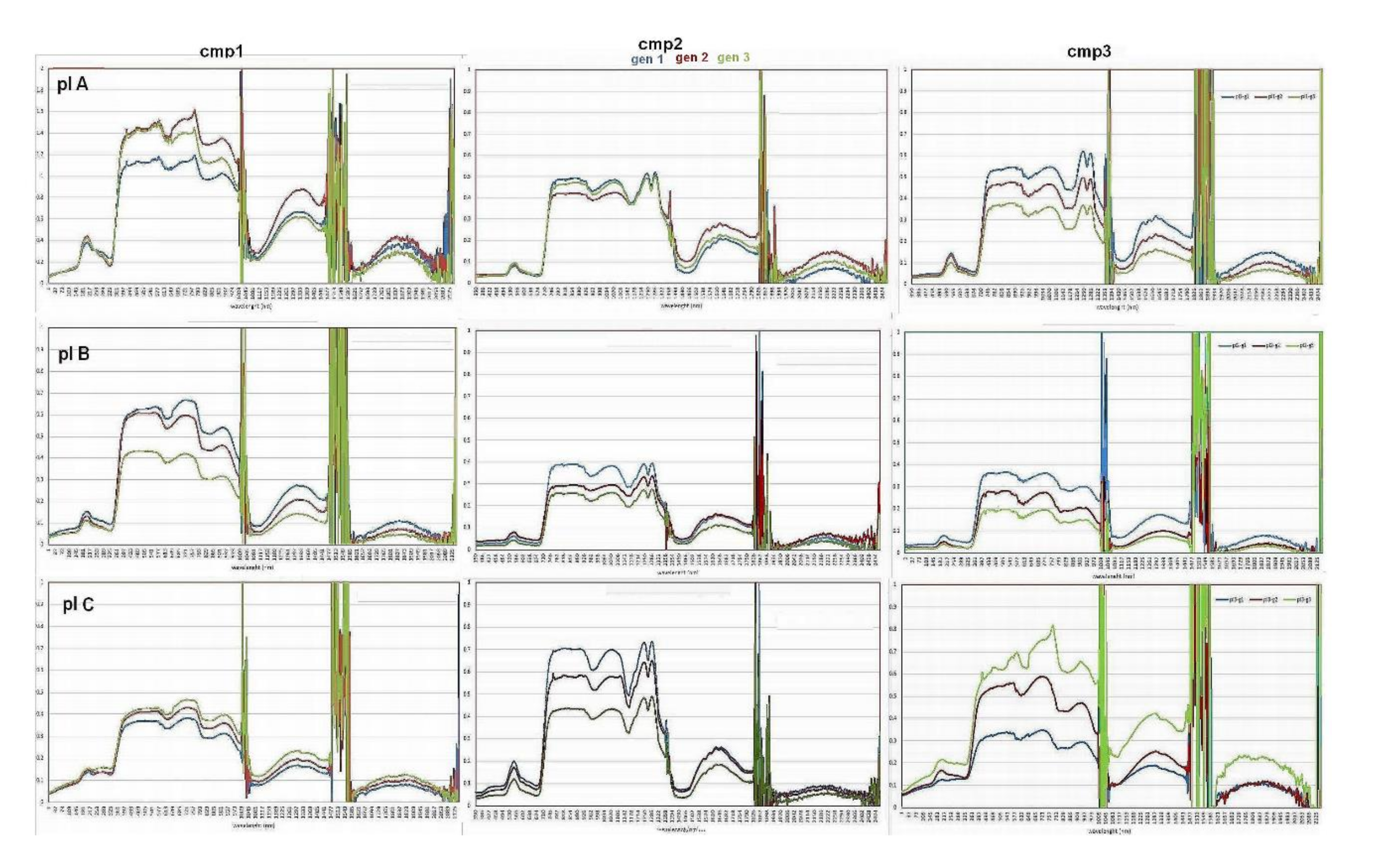
Figure 5 show the canopy hyperspectral signatures averaged for each of the three cardoon genotypes growing in the plateaus A, B, C, with rising water salinization concentrations, for all three campaigns. The similar graphs obtained from leaf spectral signatures were reported in the auxiliary materials (Figure A2). The graphs along the column show the hyperspectral signatures of cardoon genotypes growing at different salinization degrees in the three campaigns. All graphs highlight the instabilities of the reflectance values recorded around the 1380 and 1890 nm wavelength ranges corresponding to air water vapor effects, with reflectance rapid variations exceeding the physical threshold (0, 1). In addition, as shown in the graph of the first campaign (cmp1), for plateau A (pl A), the effects due to the calibration fault led to unreliable reflectance values higher than 1. The spectral signatures of the different genotypes are sufficiently distinguishable in all the graphs, while those referred to plateaus A and B demonstrated a general decrease in spectral VIS responses and increase in NIR ones in the subsequent campaign, according to the increase in the chlorophyll absorption and leaves number of developing plantlets. The plants developed with the highest water salinization (pl C) showed instead an inverse distribution of the genotype hyperspectral signatures in the first (cmp1) and in the last (cmp3) measurement with an agreement on their trends of intermediate campaign (cmp2). In the first campaign, the development of most plants is in the early stages, and due to their low LAI values, the background reflectance contribution was significant. In the second campaign, the hyperspectral reflectance curves of the different plant genotypes stabilized and increased their differentiation in the third one.
Although most of the undesirable effects of noise above evidenced were corrected and mitigated in a pre-processing step, the exploitation of hyperspectral signatures under the form of normalized ratio spectral indices allowed us to further reduce this problem.
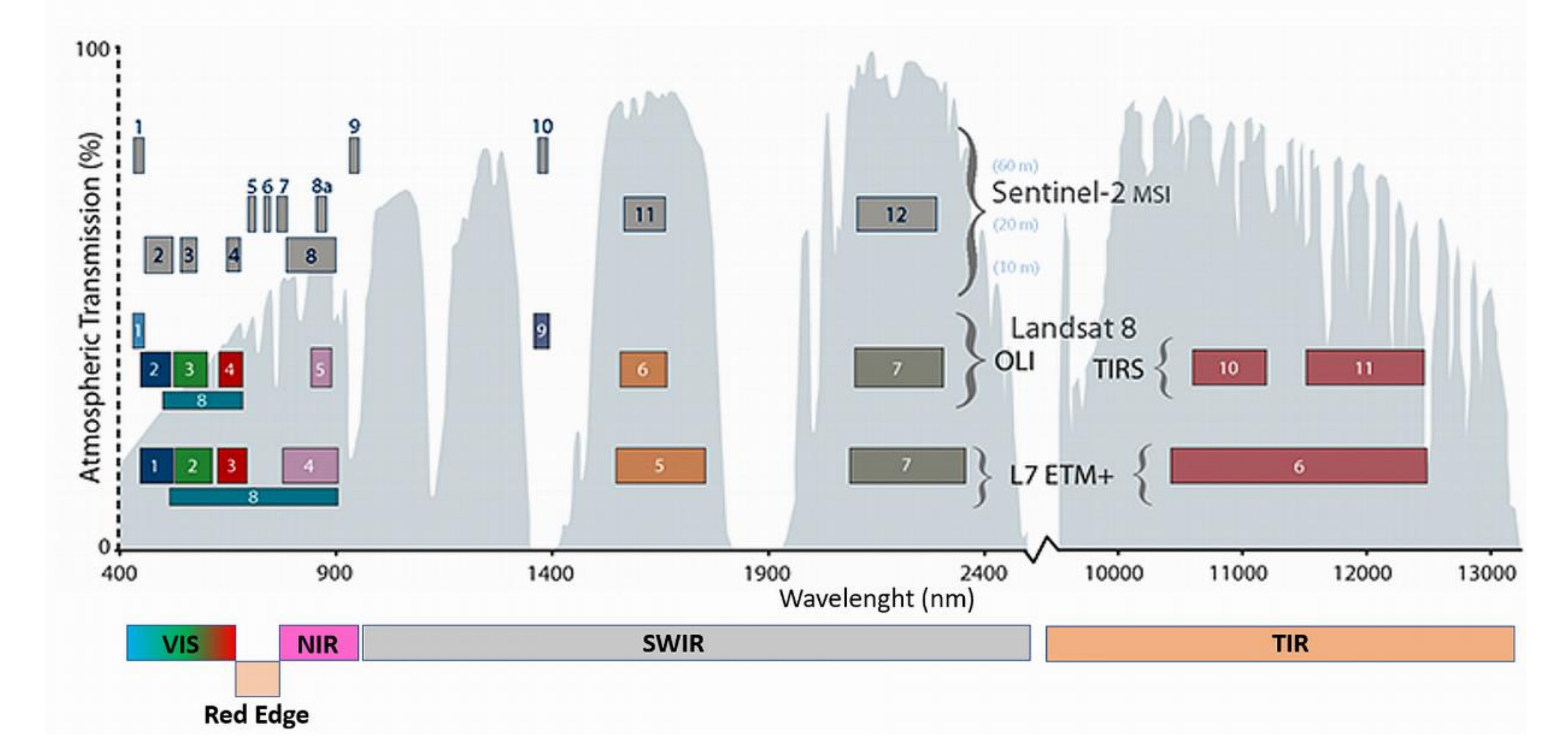
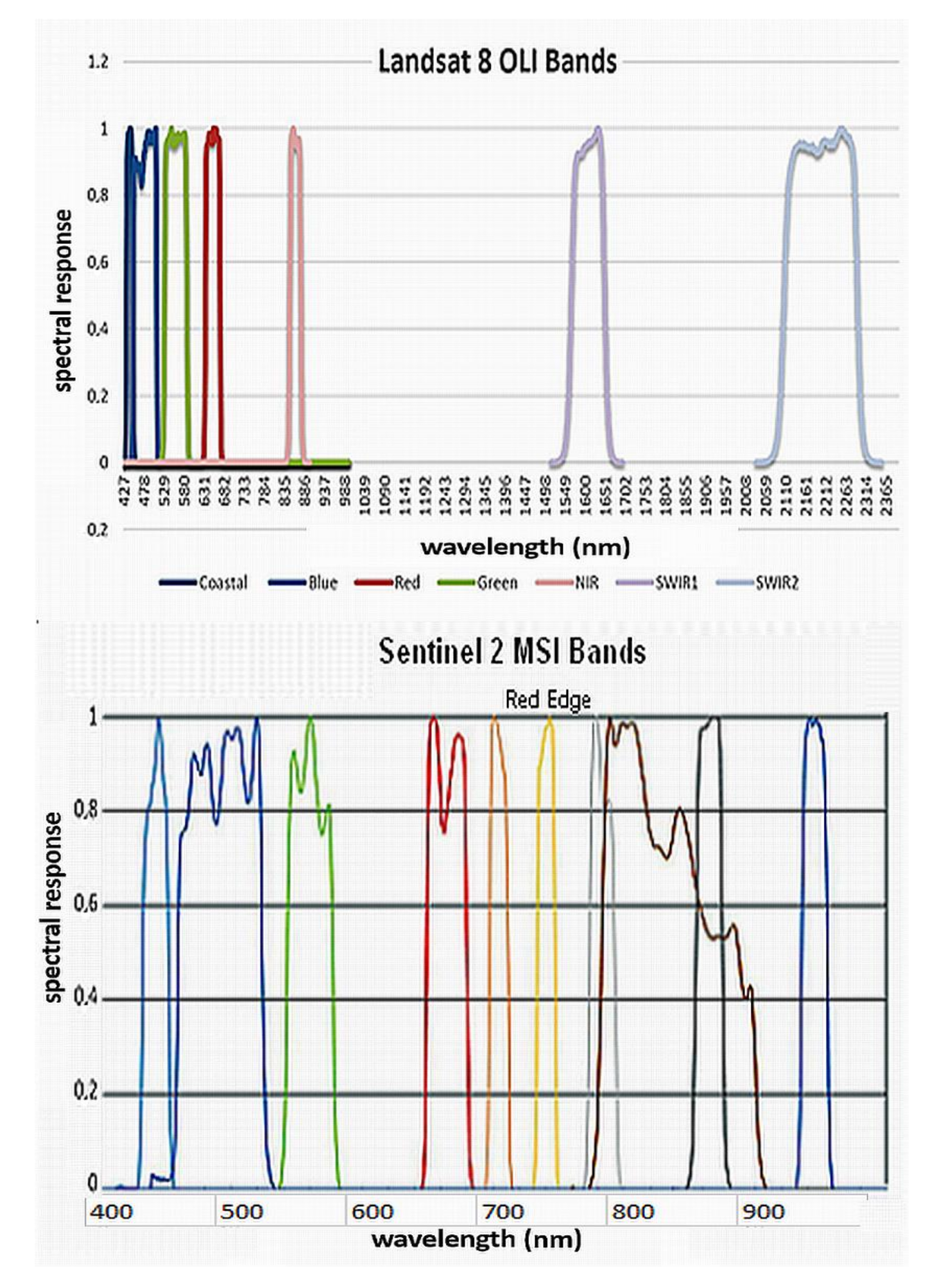
All the leaf and canopy (narrow band) indices introduced above were derived from the pre-processed hyperspectral data, then also the broadbands ones were assessed using the Landsat 8 OLI and Sentinel 2 MSI spectral bands’ filter functions (Figure A1). The results obtained from the two-factor ANOVA analysis, through Tukey’s test, were summarized in Table 4. For each of the selected spectral indices, the table includes the number of combination pairs referred to the plateau (plat. label) and genotype (gen. label) found significantly different (discriminated) in terms of means (p-values < 0.05). Table 5 and Table 6 show instead the number of pairs discriminated by the broadband indices (at canopy level) assessed, respectively, for the L8 OLI and S2 MSI satellite sensors. The corresponding ANOVA detailed p-value tables for all the indices were provided within the Appendix A (Table A4, Table A5, Table A6, Table A7, Table A8, Table A9 and Table A10). The number of discriminated combination pairs of each spectral index in the different measurement campaigns was then used as a proxy of its effectiveness in capturing the effects of the three water salinization levels on the three cardoon genotypes.
Globally, the canopy indices were found to perform better than those assessed by leaf measurements, especially in the most advanced development stages (cmp3), where only the NDVI, NPCI, SIPI RIRE, NDVI1, NDWI1 indices remain sensible to different salinization concentration at leaf level. The behavior of most leaf indices was significantly sensitive to the salinization level (plat label) in the first plant development stages (cmp1, cmp2) while once the plants were sufficiently grown, their capability to capture the effects of different water salinization levels (cmp3) decreases. In general, the leaf spectral indices capability to discriminate the spectral effects of the water salinization level on different genotype is poor, only the NDVI, TVI, SIPI, RIRE, NDVI1, NDWI1 and NDWI2 leaf indices were sensible to genotype effects at leaf level in the first growth stage (cmp1). Their capability to discriminate the effects due to the different cardoon genotypes becomes null (Table 4 leaf reflectance side) in the subsequent development phases (i.e., cmp2, cmp3). Among the foliar spectral indices sensible only to the water salinization effects on cardoon, the most performant, in the 3rd development phase (cmp3) were neatly the RIRE and NDWI (able to discriminate, respectively, two and three of index combinations pairs), with the others at the same level of performance (Table 6). Leaf indices seem mostly ineffective to capture the most subtle responses related to genotype differentiation in more advanced development stages coupled with a poorer effectiveness in detecting spectral effects of water salinization. In fact, at leaf level, only the RIRE was found capable of discriminating the spectral effects of all three levels of water salinization corresponding to three growing plots in the 3th measurement campaign (Table 4).
Contrary to their leaf counterparts, the canopy spectral indices discrimination power of spectral effects linked, respectively, to water salinization level and genotype, increases with the development stage, according to the amplification of the spectral effects of the 3-d vegetation architecture growth compared to those of single leaves. In fact, all the models related to the selected canopy spectral indices became significant in the last development stage (cmp3, canopy reflectance side), with the effective ability of all indices to discriminate the water salinization effects, coupled with higher ability for 9 of them to capture also spectral effect differentiation related to the three cardoon genotypes (Table 4, cmp3). The performance of these latter indices, evaluated for the cmp3 data by Tukey’s test, was reported in the canopy reflectance side of Table 6. These achievements demonstrate that the OSAVI and TCARI indices were able to discriminate the spectral effects related to all water salinization levels, while SAVI, TCARI, and TVI were the most sensible to differentiations in the genotype spectra, with two pairs discriminated. Finally, the most effective index in discriminating the different levels of salinization of the water and the different cardoon genotypes was the TCARI, with its total score of five (three water salinization level + two genotype combination pairs discriminated). In the “total” column of Table 4, the total sum of the combination pairs discriminated was reported as proxy of global performance of the index (for both genotype and plateau factors at leaf and canopy level). Between the structural indices, the SAVI scored the maximum number of discriminated pairs for both plateau and genotype factors, at leaf and canopy level, while TCARI resulted in the best performing of chlorophyll/pigment indices with a superior score number. Globally, also the red-edge indices have shown a good effectiveness with RE2 and REIP2 that maintained a significant performance in discriminating spectral effects of water salinization for different genotypes in the second measurement campaign. Despite its scarce capability to detect the spectral effects due to different genotypes, the NDWI of water spectral indices resulted in the best performing respect to all others. The global score, as number of discriminated pairs for both plateau and genotype combination pairs, at leaf and canopy levels, assessed for each spectral index ranges between 7 and 13, with many indices of the four groups gathering an intermediate value (9–10).
Most of L8 OLI structural indices have shown their effective capability to detect the spectral differences due to effects of different water salinization levels during all the plant growth phases (Table 5). The other chlorophyll/pigment and water indices performed well only in the early and late stages. Their discrimination capability of spectral differences due to different genotypes is weak and limited to the advanced development stage. The SAVIL, EVIL, and NPCIL were the best overall in terms of total number of discriminated pairs.
The Sentinel 2 MSI structural indices showed mostly a similar trend in detecting water salinization spectral effects (Table 6) to which we added the useful capability of those based on Red-Edge Inflection Point (REIP) working also in intermediate and advanced stages of plantar development. The capability to detect the most subtle spectral differences in the three cardoon genotypes due to water salinization levels (gen) remains weak and limited to intermediate and advanced plant growth stages. The most performant indices, which reached a total score of six combination pairs discriminated, were SAVIS, NPCIS, NWI1S, and the red-edge-based that demonstrated also the ability to detect genotype spectral differences both at the intermediate and advanced stages of plant development.
The different leaf and canopy hyperspectral indices through the data acquired during the three measurement campaigns evidenced a wide range of spectral indices sensibility, at plateau and genotype levels. In the early stage (cmp1), both the leaf and canopy indices demonstrated a useful capability to detect the plant spectral differences induced by the three water salinization levels, while only water coupled with some structural and pigment indices was found able to capture the effects at the genotype level. In the following stage (cmp2), contrary to canopy indices, the leaf ones maintained their aptitude to discriminate the effects of water salinization level without genotype distinction.
In the later stage (cmp3), the sensibility of the canopy indices, especially those of the structural and pigment ones including the genotype effects increased, while diminishing the reactivity of the leaf indices decreased. Similar trends were found for the S2 MSI broadband indices with additional capabilities demonstrated by those based on the red-edge, acquisition channels (Figure 4). Both the OLI and S2 broadband indices demonstrated a suitable aptitude to detect the spectral effects of water salinization levels on cardoon plants, especially in early and sufficiently developed stages (1.2–1.4 stages of BBCH scale), with a weak additional sensitivity to different genotypic effects of water indices in these latter.

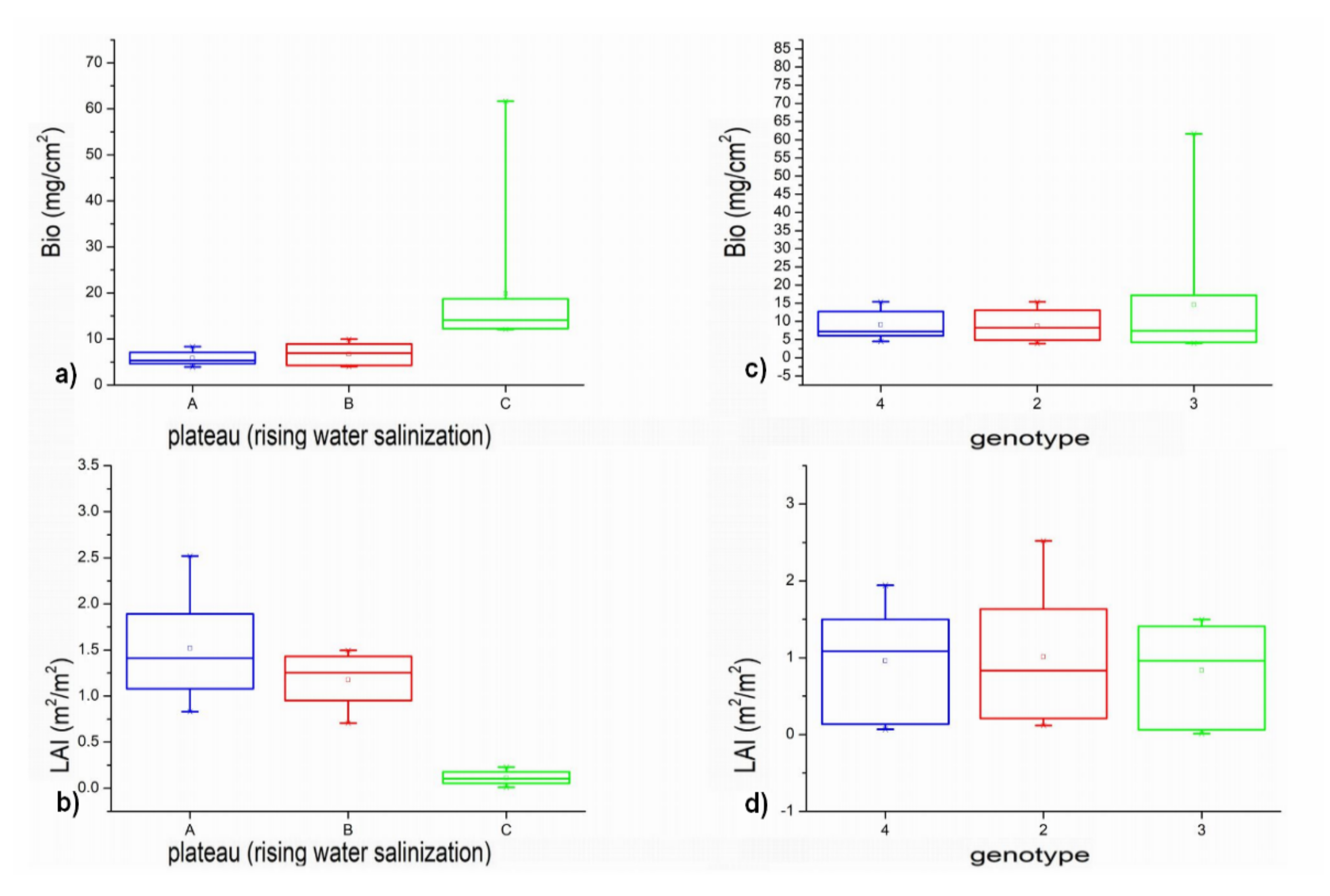
3.3. Biometry Modelling

Figure 6 shows the boxplot graphs related to Biomass (mg/cm2) and LAI (m2/m2) biometric measurements derived from cardoon samples acquired on field during the second campaign (cmp2). The graphs a and b show data related to the three plateaus with different water salinization levels (starting from A with lowest salinization to C with the maximum one). The graphs c and d show the boxplots assessed for the three different C. cardunculus genotypes.
The average trend of LAI and biomass density (Bio) do not show significant (at 95% of confidence level) variations between plateaus A and B, with raising water salinization, while the differences get significant for samples of C plateau (p-value < 0.05). This find is confirmed also by the results of Tukey’s test in Table 7, where only the two pairs A-C and B-C of LAI/Bio mean values were discriminated at plateau level, while no significant variation was found for samples of different genotypes (p-value > 0.05).
In agreement with these results, most of canopy indices of the second campaign show significant differences only at plateau level, while a weak discrimination of genotype effects was shown only by red-edge and water spectral indices (Table 6, canopy reflectance, cmp2). Similar trends were found for the OLI and MSI broadband indices.
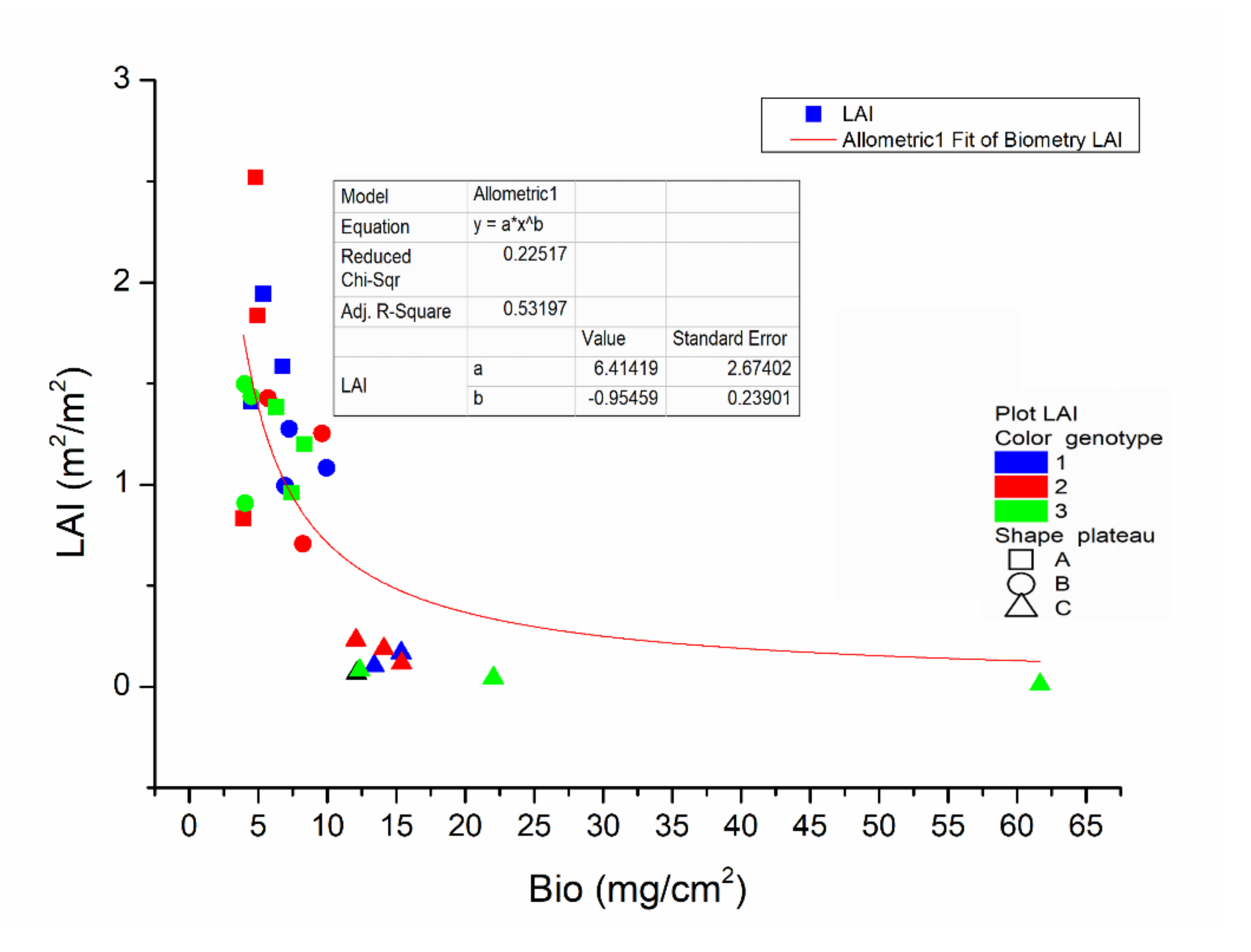
Figure 7 shows the plot of the biomass density (Bio) and the corresponding LAI measurements including their best-fit allometric curve as:
LAI = 6.4141   Bio 0.954
with the significant correlation found between them evidenced by an R2adj (adjusted correlation coefficient) = 0.53197. The LAI shows a rising trend linked to that of the lowering Bio, depicted by the fitting allometric curve, with the best-fit intermediate LAI values around 1.25. The Bio variable measurements registered the maximum in case of the smallest leaf development caused by water salinization increase, in particular for the 3rd genotype whose values are the highest ones. The distribution of measurements from the samples of the C plateau (triangular dots) is mainly located in the area near the origin of the axes, in the lower left corner of the graph (average LAI = 0.112). The other data, referring to decreasing water salinization levels, spread along the best-fit curve, with those related to the B plateau (mean LAI = 1.175) and those from the A plateau above them (mean LAI = 1.518). From this graph and from the previous analyses of the biometric data, it appears that, above a water salinization threshold (i.e., water salt concentration of the plateau C), the global development of cardoon plants is significantly inhibited, while under this threshold, the water salinization neither affects the development of the leaf surface (LAI) nor the biomass density (Bio) of 
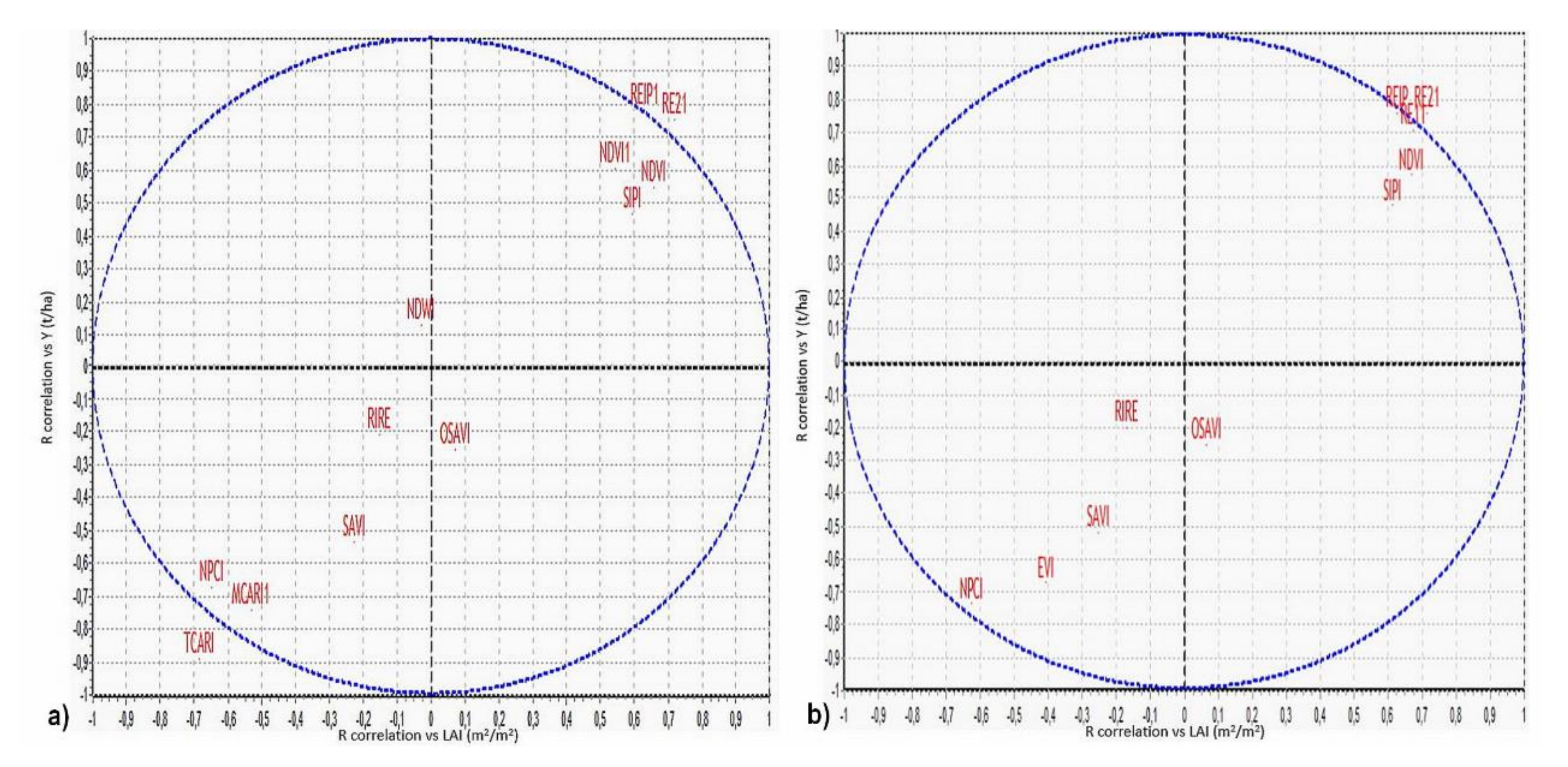
C. cardunculus plants. In order to link the biometric data to the corresponding spectral indices for modelling purposes, both the average values at genotype and plateau levels have been assessed from the related measurement datasets. In particular, the leaf and canopy hyperspectral indices and the broadband ones of the second campaign have been selected to be extensively tested for linear modelling of the yield Y, derived from measured LAI and Bio biophysical parameters (Equation (1)). The results of this modelling approach were reported below, under the form of bi-dimensional scatter plots where the coordinates of each index are the R correlation (Spearman) coefficients derived from the linear model of Y (y-axis) and LAI (x-axis) parameters, more directly linked to biomass resources on field by the bioenergetic crops. In particular, Figure 8a shows the scatter plots for canopy hyperspectral indices, while Figure 8b includes that assessed for the Sentinel MSI broadband indices. In the graphs, some spectral indices that overlap each other are not reported to avoid confusion and improve the clearness of distributions. In general, in all the graphs, the position related to all indices is distributed along the bisector of the second and third quadrants, which means that the correlations of the spectral indices with LAI and Y may have the opposite sign depending also on the implicit contribution of Bio in Y without significant differences among the three genotypes.
As reported in graph a of Figure 8, the correlation of the red-edge (REIP, RE21, RE11) canopy’s spectral indices, with the LAI/Y is positive and significant, with that slightly inferior of NDVI, NDVI1, and SIPI. The soil corrected SAVI and OSAVI, RIRE, and the NDWI indices showed instead poor correlation values with those of SAVI inferior of others and negative for both LAI and Y. The other indices (MCARI and NPCI) are characterized by a varying negative correlation with TCARI reaching the minimum values.
Most of the S2 broadband spectral indices (Figure 8, graph b), presented a behavior similar to that of the corresponding hyperspectral canopy index, with those red-edge-based (RE11, RE12, REIP) more concentrated and having the maximum positive correlation with LAI and Y. Contrary to NDVI, the EVI index, specifically designed for HR satellite optical sensors (to minimize soil and atmospheric noise contribution), shows a negative correlation, probably due to the overcorrection of absent atmospheric effects, based on blue channel. The correlation of the OLI spectral indices showed a trend similar to that of the S2 MSI, with the NDVI achieving the maximum positive correlation but inferior to that of S2 red-edge ones. In general, from these preliminary R correlation test, the red-edge indices evaluated for the second field campaign (cmp2) happened most suitably in modelling the Y biometric data (Figure 8a,b), maintaining at same time a discrimination capability for the corresponding effects of different water salinization levels (Table 6, canopy reflectance indices, cmp2).
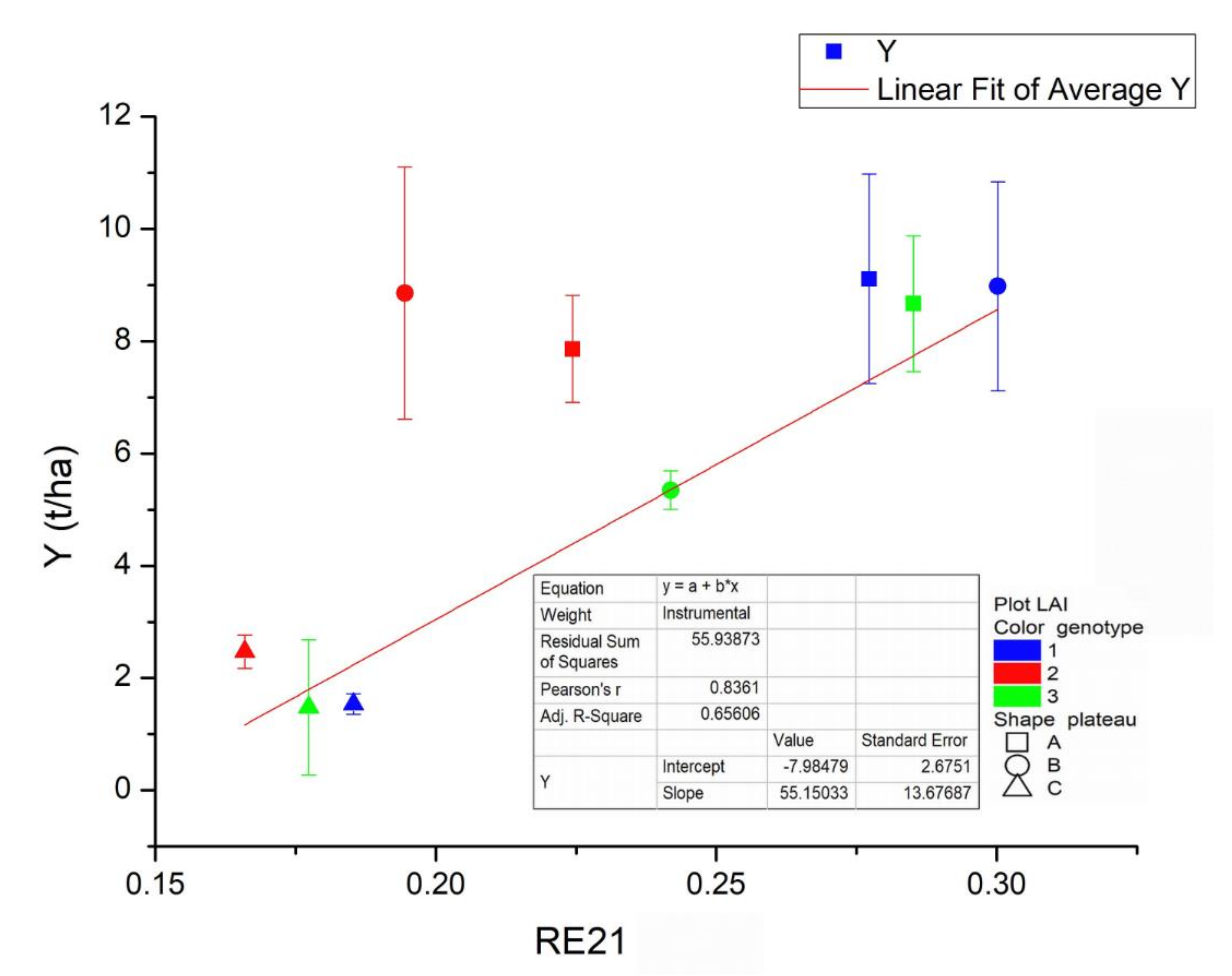
The most relevant positive correlation with Y and LAI is provided by the RE21 index, normalized difference red-edge index that reached the maximum value, followed by RE11 (Figure 8). The biomass production assessment at field level requires spatial modeling of the yield Y, in order to provide input for sustainable management and bioenergy exploitation. In this perspective, a deeper analysis of this index was carried out considering that currently the hyperspectral and multispectral data collected remotely of the areas of interest for spatial distributions assessment can be provided by the airborne or satellite operating platforms (i.e., S2 MSI satellite). Figure 9 shows the average trends of the Y derived from the biometric data and the corresponding RE21 values for each plateau (different dot shape) and genotype (different dot color). The regression equation found is:
Y = 55.15033   RE 21 7.98479
The R2 correlation of the related Y-RE21 linear model scored 0.836 (R2adj = 0.656) that means an effective capability to capture the above-ground biomass spatial variations supported by a model significance better than 95% (F-value = 16.26, Prob > F = 0.00498). The lowest Y (around 1.5 t/ha) and RE21 values were found for the cardoon plants of the three genotypes of the C plateau (triangular dots) fed with the most salinized water. The maximum (around 9 t/ha), instead, has been reached both by the first cardoon genotype grown in water at intermediate salinization (circle black dot) or not salinized water (square black dot) and by the second genotype (circle red dot) irrigated with water at intermediate salt concentration. The Y of plants of genotype 1 (black dots) and 2 (red dots), grown using water at intermediate salt concentration, approaches 9 t/ha (maximum); in particular, the Y of genotype 2 exceed that obtained with water non-salinized (about 8 t/ha).
The RE21 index and the corresponding Y values of all cardoon genotypes feeding with the most salinized water are rightly the lowest (triangular dots), but they differ in the trends of the remaining plateau. In fact, although the Y rising trend of the genotype 1 (black dots) is in agreement with water salinization reduction, the Y and RE21 index values corresponding to water middle salinization level (circle dot) were found too high respect to those of the genotype 3, while the genotype 2 showed a similar Y value compared to a significantly lower index. All the plateau averages of the genotype 3 (green dots) are rightly located along the fitting line, with Y related to middle water salinization significantly smaller than the other two and that obtained through the non-salinized water located between the others corresponding two. All the plateau Y averages of the second genotype (red dots) are located above and at a significant distance from the red line of best fit with the yield Y corresponding to the intermediate water salinization (red circle dot) higher than that of the plants fed with no salinized water (red square dot), which present an inversion not evidenced by the trends of the measurement of the other two genotypes.
A similar trend was found for the RE21s index, derived from the S2 MSI broadband spectral responses, with a higher R2 correlation coefficient and the remaining modelling parameters reported in Table 8, including those stating the relevant model confidence level.
Although the ANOVA analysis of biometry data did not evidence significant differences of genotypes’ responses to three water salinization levels, the Y biomass growing trends of genotypes 1 and 3 were found in raw agreement each other and with water salinization decreasing, except for intermediate values, corresponding to different rises in Y and corresponding RE21 index. In particular, the Y and RE21 intermediate values of this genotype (black circle dot) approaches those referring to those obtained for no salinized water (black and green square dot). The plants of 2nd genotype (red dots) instead, after a more relevant growth of the Y related to intermediate water salinization (similar to that of genotype 1 but without a corresponding rise in RE21 index) show a decreased Y respect to the same genotype thistle grown with water not salinized. In addition, these plants presented a rise in corresponding RE21 (square red dot), equivalent to around one half respect to others without water salt concentration. These results show that, at irrigation water salt concentrations of 200 mM/L (plateau C), the growth of all thistle genotypes used here is significantly inhibited both in term of Y and spectral indices responses (Y = 1–2 t/ha), while at half concentrations (plateau B), the different genotypes exhibit different behaviors. In particular, the plants of genotype 1 and 2 (black and red circle dots) evidence productivity growth (Y = 9 t/ha) approaching those obtained for genotype 1 and 3 (black and green square dots), with water not salinized (plateau A). The Y values corresponding to the plateau A for genotypes 1 and 3 look quite similar, while that of the 2nd genotype diminishes respect the corresponding Y amount of plateau B (100 mM/L).
Ultimately, from these preliminary findings, the intermediate salt concentration around 100 mM/L seems to have a negative impact on the productivity Y of the cardoon genotype 3, not affecting that of the genotype 1 and favoring the development of the second genotype used here. Although the intermediate water salinization feeding involves a rise in RE21 spectral index responses of plants of all three genotypes, their growth amount differs. The plants of the cardoon genotype 2 exhibit the smallest index value, those of the cardoon genotype 3 presented intermediate RE21 values, while the highest were assessed for the genotype 1 plants. From the comparison with the data referred to samples irrigated without salinized water, we can evidence that the 100 mM/L concentration does not impact on the Y of cardoon genotype 1, while it improves productivity of the genotype 2 (of about 1 t/ha) and inhibits that of the genotype 3 (of about 3 t/ha), as can be derived from the differences in y-coordinates in the graphs. In any case, it should be highlighted that, although Y (t/ha) is specifically linked to the production of extensive field cultivation, its estimated maxima values in our controlled and limited experimental context (about 10 t/ha of above-ground biomass) are roughly compatible with those reported in the literature for bioenergy productions growing in the field at comparable agronomic condition and with low fertilizer inputs, taking into account also of biomass partitioning between leaves, stalks, and heads and wet/dry mass mutual dependence [6,9].

4. Conclusions

Cardoon exploitation as a bioenergy resource is widely diffusing, particularly in the Mediterranean basin, due to its relevant annual biomass yield with a low request of inputs and a significant resilience to stresses due to drought and water shortage, soil/water salinization, and soil pollution. This crop may have a wide range of bio-industrial applications and fit into different intensive cultivation strategies that can be improved by precision farming approaches, supported by the currently available remote and proximal sensing techniques, including those exploiting EO data continuously provided by orbiting satellites. In this perspective, various spectral vegetation indices based on these remote sensing techniques tested here have demonstrated their ability to discriminate between the spectral differences induced on cardoon plants by different water salinization levels (at leaf and canopy level) at the different growth stages. The more difficult detection of subtler spectral effects of water salinization on the different cardoon genotypes was anywhere provided by different indices in the various development phases. Even if, as expected, the tested broadband spectral vegetation indices showed a slightly lower capability, they maintained an appreciable discrimination of the spectral effects due to three salinization levels in irrigation water of cardoon growing plants with a weak capability to differentiate the genotype effects. The red-edge-based indices demonstrated also a good modelling capability of biometric parameters derived from the field data as the yield, Y (t/ha). The useful cardoon Y (t/ha) modelling capability, demonstrated by narrow/spectral vegetation indices broadband tested here (in particular by red-edge-based ones), in perspective, can support effective, repetitive, and extensive monitoring of these bioenergetic crops by providing early detection and mapping of plan stresses and health that can have an impact on production. In the framework of precision farming approach, these information are the basis for sustainable and effective management with space-variant interventions (even supported by semi-autonomous agricultural VRT—variable rate technology machinery) for optimizing the production minimizing at same time external inputs and environmental impacts. The current wide availability of HR satellite multispectral data, remotely detected in the various spectral ranges, including the red edge one (i.e., S2 MSI), with the realistic perspective of exploiting the available satellite hyperspectral sensors (PRISMA, ENMAP), provide very useful monitoring opportunities of cardoon and other bioenergy crops. Although the noise effects due to atmospheric disturbance and the sun-view anisotropy (minimized through acquisition geometry and normalized spectral indices exploitation) have not been taken into account here, the satellite broadband indices in different wavelengths evaluated have preliminarily proven to be potentially useful for extensive and effective cardoon monitoring. In addition, the remote/proximal sensing techniques tested here could support the further extensive characterization of cardoon production, including the quantification of seeds and biochemical substances and compound concentrations within a biorefinery context, with the selection of suitable genotypes for biomass production also characterized by a different degree of the chlorine absorption, which is a further undesirable factor to be taken into consideration for the processes for bioenergy production.

5. Reference Projects

The present research has been conducted within the framework of:
  • Multi-year national program of National Electric System Research (RdS) financed by the MISE (Ministry of Economic Development) for research and development activities in the electricity sector and to improve its cost-effectiveness, safety, and environmental compatibility, with funding to ENEA for the development of models and technologies to assess and reduce anthropogenic impacts and natural hazards arising from energy production, in particular for the implementation of innovative monitoring methods based on Earth observation techniques;
  • REBIOCHEM project, funded by the Italian Ministry of Education, University and Research for the cluster on Green Chemistry, focusing on assessing the potential of different cardoon species and genotypes in terms of biomass production and extraction of useful compounds from raw materials, within the biorefinery context.

Author Contributions

Methodology: F.B., C.M., L.D.C., and D.M.; experimental design and setup: P.C., A.C., and A.F.; data acquisition and analysis; F.B., C.M., L.D.C., D.M., D.I., and L.B.; field work activity: L.D.C., A.F., A.C., and D.I.; writing and editing the original manuscript: F.B., L.D.C., and D.I. All authors contributed to its first review with figure and graph production under the supervision of F.B. and V.P. All authors have read and agreed to the published version of the manuscript.

Funding

National program of National Electric System Research (RdS); REBIOCHEM project.

Conflicts of Interest

The authors declare no conflict of interest. ENEA is not responsible for any use, even partial, of the contents of this document by third parties and any damage caused to third parties resulting from its use.

Appendix A

Table A1. Abbreviation, expressions and acronyms.
ExpressionDescription
(Adjusted) R square(Adjusted) R2 correlation coefficient
a.g.r.Above ground resolution
ANOVAAnalysis of Variance
BBCHBiologische Bundesanstalt, Bundessortenamt, CHemischeIndustrie
BioLeaf biomass density (mg/cm2)
bxBroadband spectral response in band/spectral range x
cmpnMeasurement campaign (n:1, 2, 3)
DFDegree of Freedom, i.e. number of measurements minus parameters
Fact.ANOVA factor
F ValueANOVA F statistic
fijBroad band j filter function
genCardoon genotype
LAILeaf Area index
mM10−3 moles
MSIMultiSpectral Instrument
NIRNear Infrared
OLIOperational Land Imager
platplateau
Pl XPlateau at different water salinization levels (X: A, B, C)
Prob > Fp-value for the whole regression model
p-valueSignificance level of single factor/global relationship model
RR Spearman correlation coefficient
redgRed Edge
rxNarrow band spectral reflectance in band x
SNRSignal to noise ratio
SWIRShort Wave Infrared
TIRThermal Infrared
Typ.Typology
UvUltraviolet
VISVisible
YBiomass yield (t/ha)
Table A2. Landsat 8 OLI acquisition bands. The band width is evaluated as FWHM (Full Width Half Maximum) of the related filter function.
BandsLandsat 8 OLI BandCenter Wavelength (nm)Band Width (nm)Spatial
Resolution (a.g.r.) m
b1Coastal442.9615.9830
b2Blue482.0460.0430
b3Green561.4157.3330
b4Red654.5937.4730
b5NIR864.6728.2530
b6SWIR11608.8684.7230
b7SWIR22200.73186.6630
b8Pan589.50172.4015
b9Cirrus1373.4320.3930
Table A3. Sentinel 2 MSI acquisition bands. The band width is evaluated as FWHM (Full Width Half Maximum) of the related filter function.
BandsSentinel-2 MSI BandsCentral
Wavelength
(nm)
Band
Width
(nm)
Spatial
Resolution
(a.g.r. m)
b1Band 1: Coastal 4432060
b2Band 2: Blue4906510
b3Band 3: Green5603510
b4Band 4: Red6653010
b5Band 5: Red-edge 17051520
b6Band 6: Red-edge 27401520
b7Band 7: Red-edge 37832020
b8Band 8: NIR84211510
b9Band 8A: NIR narrow8652020
b10Band 9: Water Vapor9452060
b11Band 10:SWIR Cirrus13753060
b12Band 11: SWIR16109020
b13Band 12: SWIR219018020
Table A4. p-values obtained from two way ANOVA analyses of structural/LAI and Chlorophyll/pigments leaf hyperspectral indices. The values lower than 0.05 have been reported in bold.
cmpFact.NDVISAVIOSAVITCARITVISIPINPCIMCARI1
1gen6.19 × 10−47.51 × 10−11.43 × 10−19.61 × 10−15.52 × 10−31.28 × 10−41.19 × 10−17.47 × 10⁻¹
plat3.24 × 10−52.87 × 10−71.85 × 10−42.92 × 10−39.98 × 10−12.31 × 10−32.17 × 10−53.51 × 10⁻²
model1.33 × 10−63.11 × 10−63.65 × 10−41.83 × 10−23.25 × 10−21.15 × 10−55.86 × 10−51.16 × 10⁻¹
2gen2.79 × 10−13.72 × 10−13.59 × 10−14.77 × 10−13.63 × 10−12.63 × 10−15.42 × 10−13.77 × 10⁻¹
plat1.60 × 10−52.60 × 10−24.80 × 10−32.40 × 10−61.15 × 10−31.23 × 10−51.95 × 10−53.70 × 10⁻⁴
model7.77 × 10−55.76 × 10−21.39 × 10−21.72 × 10−54.10 × 10−35.93 × 10−51.28 × 10−41.54 × 10⁻³
3gen1.49 × 10−11.82 × 10−11.35 × 10−11.78 × 10−11.49 × 10−11.30 × 10−19.81 × 10−11.64 × 10⁻¹
plat4.44 × 10−32.47 × 10−11.52 × 10−13.63 × 10−11.75 × 10−14.52 × 10−33.42 × 10−29.43 × 10⁻²
model7.98 × 10−31.93 × 10−11.12 × 10−12.47 × 10−11.33 × 10−17.45 × 10−31.32 × 10−19.08 × 10⁻²
Table A5. p-values obtained from two way ANOVA analyses of Red-Edge and water content leaf hyperspectral indices. The values lower than 0.05 have been reported in bold.
cmpFact.RE1RE2RE11RE21RIRENDVI1REIP1REIP2NDWINDWI2
1gen6.08 × 10−16.67 × 10−12.95 × 10−14.67 × 10−11.16 × 10−31.35 × 10−28.02 × 10−17.89 × 10−14.01 × 10−41.49 × 10⁻⁵
plat4.53 × 10−47.12 × 10−86.25 × 10−112.45 × 10−134.80 × 10−113.75 × 10−137.15 × 10−127.23 × 10−120.001.96 × 10−11
model2.35 × 10−37.45 × 10−76.12 × 10−103.94 × 10−121.75 × 10−119.32 × 10−131.33 × 10−101.34 × 10−100.005.42 × 10−13
2gen3.78 × 10−15.13 × 10−12.09 × 10−11.26 × 10−12.04 × 10−19.36 × 10−22.17 × 10−12.17 × 10−14.48 × 10−12.29 × 10⁻¹
plat1.48 × 10−24.94 × 10−21.08 × 10−64.84 × 10−86.74 × 10−11.71 × 10−41.55 × 10−61.55 × 10−62.29 × 10−41.22 × 10⁻¹
model3.68 × 10−21.19 × 10−15.76 × 10−62.68 × 10−74.05 × 10−13.56 × 1048.17 × 10−68.17 × 10−61.10 × 10−31.35 × 10⁻¹
3gen1.55 × 10−11.76 × 10−11.24 × 10−14.46 × 10−23.14 × 10−51.61 × 10−19.18 × 10−19.17 × 10−11.38 × 10−113.19 × 10⁻²
plat1.40 × 10−12.21 × 10−17.72 × 10−18.89 × 10−19.72 × 10−18.48 × 10−15.98 × 10−15.17 × 10−11.44 × 10−12.13 × 10⁻¹
model1.16 × 10−11.75 × 10−13.08 × 10−11.54 × 10−12.39 × 10−43.92 × 10−18.71 × 10−18.18 × 10−11.21 × 10−104.80 × 10⁻²
Table A6. p-values obtained from two way ANOVA analyses of structural/LAI and Chlorophyll/pigments canopy hyperspectral indices. The values lower than 0.05 have been reported in bold.
cmpFact.NDVISAVIOSAVITCARITVISIPINPCIMCARI1
1plat3.79 × 10−63.94 × 10−71.27 × 10−66.55 × 10−81.002.69 × 10−76.80 × 10−44.62 × 10−8
gen1.30 × 10−12.33 × 10−11.85 × 10−14.77 × 10−12.41 × 10−11.10 × 10−12.14 × 10−14.22 × 10⁻¹
model1.64 × 10−52.44 × 10−66.78 × 10−65.30 × 10−75.62 × 10−11.38 × 10−62.02 × 10−33.69 × 10⁻⁷
2plat1.35 × 10−11.23 × 10−23.41 × 10−21.74 × 10−21.38 × 10−13.65 × 10−14.44 × 10−11.48 × 10⁻²
gen1.94 × 10−16.42 × 10−29.59 × 10−29.22 × 10−21.95 × 10−16.58 × 10−17.57 × 10−11.34 × 10⁻¹
model1.56 × 10−11.98 × 10−24.68 × 10−22.87 × 10−21.60 × 10−15.44 × 10−16.57 × 10−12.83 × 10⁻²
3plat4.77 × 10−82.11 × 10−32.72 × 10−51.94 × 10−54.37 × 10−33.13 × 10−81.14 × 10−61.20 × 10⁻²
gen9.74 × 10−21.62 × 10−21.82 × 10−21.44 × 10−38.00 × 10−31.09 × 10−13.80 × 10−36.24 × 10⁻³
model2.69 × 10−71.17 × 10−34.09 × 10−59.35 × 10−61.26 × 10−31.86 × 10−71.57 × 10−62.11 × 10⁻³
Table A7. p-values obtained from two way ANOVA analyses of Red-Edge and water content canopy hyperspectral indices. The values lower than 0.05 have been reported in bold.
cmpFact.RE1RE2RE11RE21RIRENDVI1REIP1REIP2NDWINDWI2
1plat3.40 × 10−85.54 × 10−82.34 × 10−76.38 × 10−91.53 × 10−36.95 × 10−72.15 × 10−95.17 × 10−91.09 × 10−27.66 × 10⁻⁴
gen3.60 × 10−12.81 × 10−11.76 × 10−11.44 × 10−15.65 × 10−23.37 × 10−29.94 × 10−21.12 × 10−16.13 × 10−15.03 × 10⁻¹
model2.65 × 10−74.00 × 10−71.38 × 10−64.42 × 10−81.92 × 10−32.26 × 10−61.46 × 10−83.45 × 10−83.87 × 10−23.44 × 10⁻³
2plat1.68 × 10−23.93 × 10−29.40 × 10−23.24 × 10−25.48 × 10−15.09 × 10−21.85 × 10−21.74 × 10−25.21 × 10−19.15 × 10⁻²
gen5.21 × 10−22.45 × 10−22.04 × 10−11.08 × 10−17.95 × 10−26.35 × 10−25.04 × 10−25.12 × 10−23.35 × 10−22.49 × 10⁻²
model2.29 × 10−22.58 × 10−21.28 × 10−14.75 × 10−21.64 × 10−14.98 × 10−22.41 × 10−22.33 × 10−27.76 × 10−23.70 × 10⁻²
3plat1.86 × 10−21.40 × 10−23.89 × 10−84.31 × 10−85.75 × 10−41.19 × 10−23.16 × 10−33.77 × 10−36.42 × 10−67.75 × 10⁻⁴
gen1.33 × 10−23.86 × 10−21.04 × 10−11.24 × 10−19.14 × 10−29.27 × 10−27.44 × 10−17.62 × 10−13.89 × 10−13.93 × 10⁻²
model4.86 × 10−38.29 × 10−32.26 × 10−72.60 × 10−71.12 × 10−31.30 × 10−21.48 × 10−21.75 × 10−23.89 × 10−59.08 × 10⁻⁴
Table A8. p-values obtained from two way ANOVA analyses of Landsat 8 OLI spectral indices. The values lower than 0.05 have been reported in bold.
cmpFactorNDVILSAVILOSAVILEVISSIPINPCINWDINWI1NWI2
1plat4.21 × 10−61.68 × 10−71.01 × 10−62.31 × 10−73.36 × 10−71.86 × 10−52.49 × 10−45.29 × 10−41.01 × 10−6
gen1.57 × 10−12.58 × 10−12.00 × 10−12.77 × 10−11.35 × 10−13.34 × 10−12.87 × 10−15.68 × 10−13.85 × 10−1
model1.93 × 10−51.12 × 10−65.60 × 10−61.55 × 10−61.80 × 10−69.83 × 10−59.68 × 10−42.62 × 10−36.79 × 10−6
2plat1.10 × 10−11.32 × 10−23.71 × 10−29.31 × 10−31.24 × 10−13.59 × 10−15.20 × 10−28.65 × 10−22.25 × 10−1
gen2.02 × 10−16.19 × 10−29.09 × 10−25.19 × 10−21.81 × 10−17.61 × 10−11.75 × 10−12.72 × 10−24.16 × 10−1
model1.41 × 10−12.06 × 10−24.85 × 10−21.51 × 10−21.44 × 10−15.76 × 10−17.95 × 10−23.85 × 10−23.18 × 10−1
3plat4.14 × 10−86.96 × 10−31.57 × 10−42.46 × 10−22.97 × 10−83.77 × 10−65.29 × 10−54.21 × 10−42.42 × 10−3
gen8.04 × 10−23.20 × 10−11.88 × 10−14.21 × 10−18.48 × 10−23.09 × 10−21.30 × 10−23.61 × 10−21.50 × 10−1
model2.25 × 10−71.81 × 10−25.29 × 10−46.03 × 10−21.67 × 10−79.64 × 10−65.99 × 10−55.33 × 10−44.87 × 10−3
Table A9. p-values obtained from two way ANOVA analyses of Sentinel 2 MSI structural/LAI and Chlorophyll/pigments spectral indices. The values lower than 0.05 have been reported in bold.
cmpFactorNDVI1NDVI2NDVI3SAVIOSAVIEVISIPINPCI
1plat5.07 × 10−76.29 × 10−71.03 × 10−62.55 × 10−64.01 × 10−63.22 × 10−66.29 × 10−74.39 × 10⁻⁹
gen1.22 × 10−11.38 × 10−11.33 × 10−12.61 × 10−11.98 × 10−13.02 × 10−11.38 × 10−11.08 × 10⁻¹
model2.55 × 10−63.23 × 10−65.05 × 10−61.44 × 10−51.99 × 10−51.87 × 10−53.23 × 10−62.93 × 10⁻⁸
2plat1.25 × 10−11.16 × 10−11.51 × 10−11.29 × 10−23.42 × 10−21.02 × 10−21.28 × 10−14.08 × 10⁻¹
gen1.98 × 10−11.92 × 10−12.51 × 10−16.49 × 10−29.30 × 10−26.97 × 10−21.77 × 10−17.99 × 10⁻¹
model1.51 × 10−11.42 × 10−11.92 × 10−12.06 × 10−24.64 × 10−21.77 × 10−21.44 × 10−16.39 × 10⁻¹
3plat3.60 × 10−85.11 × 10−74.39 × 10−86.07 × 10−31.35 × 10−41.99 × 10−25.11 × 10−72.13 × 10⁻⁶
gen6.51 × 10−22.93 × 10−17.12 × 10−23.15 × 10−11.80 × 10−14.20 × 10−12.93 × 10−11.24 × 10⁻²
model1.87 × 10−73.32 × 10−62.30 × 10−71.60 × 10−24.54 × 10−45.06 × 10−23.32 × 10−64.17 × 10⁻⁶
Table A10. p-values obtained from two way ANOVA analyses of Sentinel 2 MSI Red-Edge and water content spectral indices. The values lower than 0.05 have been reported in bold.
cmpFactorRE11RE21NWDINWI1NWI2NDVI4REIP1
1plat1.58 × 10−57.17 × 10−27.84 × 10−79.53 × 10−41.25 × 10−62.29 × 10−71.00 × 10−6
gen8.06 × 10−22.27 × 10−11.41 × 10−14.74 × 10−14.54 × 10−11.11 × 10−14.09 × 10−1
model4.88 × 10−59.29 × 10−23.98 × 10−64.06 × 10−38.78 × 10−61.19 × 10−66.88 × 10−6
2plat8.54 × 10−27.10 × 10−24.35 × 10−28.79 × 10−22.10 × 10−11.24 × 10−11.88 × 10−2
gen1.95 × 10−11.57 × 10−11.72 × 10−12.70 × 10−24.13 × 10−12.02 × 10−15.19 × 10−2
model1.17 × 10−19.43 × 10−26.94 × 10−23.87 × 10−23.03 × 10−11.52 × 10−12.47 × 10−2
3plat4.14 × 10−81.09 × 10−76.74 × 10−73.69 × 10−43.36 × 10−32.14 × 10−84.33 × 10−3
gen1.08 × 10−11.09 × 10−13.07 × 10−13.21 × 10−21.45 × 10−16.59 × 10−27.60 × 10−1
model2.42 × 10−76.00 × 10−74.36 × 10−64.50 × 10−46.25 × 10−31.16 × 10−71.97 × 10−2
Figure A1. Landsat 8 OLI (upper) and Sentinel 2 MSI (lower) bandpass filter functions.
Resources 09 00124 g0a1
Figure A2. Leaf hyperspectral signatures averages for the three cardoon genotypes growing at different water salinization level (pl A, B, C) measured during the three campaigns (cmp1, cmp2, cmp3).
Resources 09 00124 g0a2

References

  1. Alsaleh, M.; Abdul-Rahim, A.S. Bioenergy Intensity and Its Determinants in European Continental Countries: Evidence Using GMM Estimation. Resources 2019, 8, 43. [Google Scholar] [CrossRef] [Green Version]
  2. Borfecchia, F.; Pollino, M.; de Cecco, L.; Martini, S.; La Porta, L.; Marucci, A.; Caiaffa, E. Integrated GIS and Remote Sensing Techniques to Support PV Potential Assessment of Roofs in Urban Areas. In Computational Science and Its Applications-ICCSA 2013; Murgante, B., Misra, S., Carlini, M., Torre, C.M., Nguyen, H., Taniar, D., Apduhan, B.O., Gervasi, O., Eds.; Springer: Berlin/Heidelberg, Germany, 2013; Volume 7973. [Google Scholar]
  3. Baibagyssov, A.; Thevs, N.; Nurtazin, S.; Waldhardt, R.; Beckmann, V.; Salmurzauly, R. Biomass Resources of Phragmites australis in Kazakhstan: Historical Developments, Utilization, and Prospects. Resources 2020, 9, 74. [Google Scholar] [CrossRef]
  4. Jekayinfa, S.O.; Orisaleye, J.I.; Pecenka, R. An Assessment of Potential Resources for Biomass Energy in Nigeria. Resources 2020, 9, 92. [Google Scholar] [CrossRef]
  5. Demirbas, A. Biofuels: Securing the Planet’s Future Energy Needs. Energy Convers. Manag. 2009, 50, 2239–2249. [Google Scholar] [CrossRef]
  6. Gominhoa, J.; Curt, M.D.; Lourenço, A.; Fernández, J.; Pereir, H. Cynara cardunculus L. as a biomass and multi-purpose crop: A review of 30 years of research. Biomass Bioenergy 2018, 109, 257–275. [Google Scholar] [CrossRef]
  7. Karkanis, A.; Bilalis, D.; Efthimiadou, A. Cultivation of milk thistle (Silybum marianum L. Gaertn.), a medicinal weed. Ind. Crop. Prod. 2011, 34, 825–830. [Google Scholar] [CrossRef]
  8. Afshar, K.; Chaichi, M.R.; Alipour, A.; Ansari Jovini, M.; Dashtaki, M.; Hashemi, M. Potential of Milk Thistle for Biomass Production in Semiarid Regions. Crop Sci. 2015, 55, 1–7. [Google Scholar] [CrossRef]
  9. Ierna, A.; Mauro, R.P.; Mauromicale, G. Biomass, grain and energy yield in Cynara cardunculus L. as affected by fertilization, genotype and harvest time. Biomass Bioenergy 2012, 36, 404–410. [Google Scholar] [CrossRef]
  10. Kayad, A.; Paraforos, D.S.; Marinello, F.; Fountas, S. Latest Advances in Sensor Applications in Agriculture. Agriculture 2020, 10, 362. [Google Scholar] [CrossRef]
  11. Aranguren, M.; Castellón, A.; Aizpurua, A. Crop Sensor Based Non-destructive Estimation of Nitrogen Nutritional Status, Yield, and Grain Protein Content in Wheat. Agriculture 2020, 10, 148. [Google Scholar] [CrossRef]
  12. Yao, X.; Yao, X.; Jia, W.; Tian, Y.; Ni, J.; Cao, W.; Zhu, Y. Comparison and Intercalibration of Vegetation Indices from Different Sensors for Monitoring Above-Ground Plant Nitrogen Uptake in Winter Wheat. Sensors 2013, 13, 3109–3130. [Google Scholar] [CrossRef] [PubMed]
  13. Borfecchia, F.; de Cecco, L.; Della Rocca, A.B.; Farneti, A.; La Porta, L.; Martini, S.; Giordano, L.; Trotta, C.; Marcoccia, S. Innovative Remote Sensing techniques for vegetation monitoring. Energy Ambiente Innov. 2008, 54, 56–69. [Google Scholar]
  14. Gaglio, M.; Tamburini, E.; Lucchesi, F.; Aschonitis, V.; Atti, A.; Castaldelli, G.; Fano, E.A. Life Cycle Assessment of Maize-Germ Oil Production and the Use of Bioenergy to Mitigate Environmental Impacts: A Gate-To-Gate Case Study. Resources 2019, 8, 60. [Google Scholar] [CrossRef] [Green Version]
  15. Borfecchia, F.; De Cecco, L.; Martini, S.; Giordano, L.; Trotta, C.; Masci, D.; Di Gioia, V.; Pignatelli, V.; Micheli, C.; Moreno, A.; et al. Integrated aerospace technologies in precision agriculture support. Energy Ambiente Innov. 2015, 61, 32–35. [Google Scholar]
  16. Hermann, J.H. Precision in Crop Farming: Site Specific Concepts and Sensing Methods: Applications and Results; Springer: Dordrecht, The Netherlands; Heidelberg, Germany; New York, NY, USA; London, UK, 2013; ISBN 978-94-007-6760-7. [Google Scholar] [CrossRef]
  17. García-Martínez, H.; Flores-Magdaleno, H.; Ascencio-Hernández, R.; Khalil-Gardezi, A.; Tijerina-Chávez, L.; Mancilla-Villa, O.R.; Vázquez-Peña, M.A. Corn Grain Yield Estimation from Vegetation Indices, Canopy Cover, Plant Density, and a Neural Network Using Multispectral and RGB Images Acquired with Unmanned Aerial Vehicles. Agriculture 2020, 10, 277. [Google Scholar] [CrossRef]
  18. Avtar, R.; Sahu, N.; Aggarwal, A.K.; Chakraborty, S.; Kharrazi, A.; Yunus, A.P.; Dou, J.; Kurniawan, T.A. Exploring Renewable Energy Resources Using Remote Sensing and GIS—A Review. Resources 2019, 8, 149. [Google Scholar] [CrossRef] [Green Version]
  19. Borfecchia, F.; de Cecco, L.; Dibari, C.; Iannetta, M.; Martini, S.; Schino, G. Ottimizzazione della stima della biomassa pascoliva nel parco nazionale dei Monti Sibillini tramite dati satellitari e rilievi a terra. In Proceedings of the 5th ASITA Conference, Rimini, Italy, 15–18 November 2001; pp. 9–12. [Google Scholar]
  20. Borfecchia, F.; Micheli, C.; Cibic, T.; Pignatelli, V.; de Cecco, L.; Consalvi, N.; Caroppo, C.; Rubino, F.; Di Poi, E.; Kralj, M.; et al. Multispectral Data by the New Generation of High-Resolution Satellite Sensors for Mapping Phytoplankton Blooms in the Mar Piccolo of Taranto (Ionian Sea, Southern Italy). Eur. J. Remote Sens. 2019, 52, 400–418. [Google Scholar] [CrossRef] [Green Version]
  21. Borfecchia, F.; Consalvi, N.; Micheli, C.; Carli, F.M.; Cognetti De Martiis, S.; Gnisci, V.; Piermattei, V.; Belmonte, A.; De Cecco, L.; Bonamano, S.; et al. Landsat 8 OLI satellite data for mapping of the Posidonia oceanica and benthic habitats of coastal ecosystems. Int. J. Remote Sens. 2019, 40, 1548–1575. [Google Scholar] [CrossRef]
  22. Borfecchia, F.; Micheli, C.; Belmonte, A.; de Cecco, L.; Sannino, G.; Bracco, G.; Mattiazzo, G.; Struglia, M.V. Impact of ISWEC Sea Wave Energy Converter on Posidonia Oceanica Meadows Assessed by Satellite Remote Sensing in the Coastal Areas of Pantelleria Island. In Proceedings of the EGU General Assembly Conference Abstracts (EPSC2016-16787), Vienna, Austria, 17–22 April 2016. [Google Scholar]
  23. Adusumilli, N.; Lee, T.; Rister, M.E.; Lacewell, R.D. The Economics of Mitigation of Water Pollution Externalities from Biomass Production for Energy. Resources 2014, 3, 721–773. [Google Scholar] [CrossRef] [Green Version]
  24. Borfecchia, F.; Cimbelli, A.; de Cecco, L.; Della Rocca, A.B.; Martini, S.; Barbini, R.; Colao, F.; Fantoni, R.; Palucci, A.; Ribezzo, S. Integrated Remote Sensing Mission, in the Venice Lagoon. Remote Sensing of Vegetation and Sea; Cecchi, G., D’Urso, G., Engman, E.T., Gudmandsen, P., Eds.; SPIE: Washington, DC, USA, 1997; Volume 2959, pp. 162–170. [Google Scholar] [CrossRef]
  25. Crinò, P.; Correnti, A.; Farneti, A.; Tolaini, V.; Ciancolini, A.; Ardito, L.; Saccardo, F. Genetic diversity of cultivated cardoon to select high biomass producing genotypes. ACTA Hortic. 2016, 1147, 57–60. [Google Scholar] [CrossRef]
  26. Archontoulis, S.V.; Struik, P.C.; Vos, J.; Danalatos, N.G. Phenological growth stages of Cynara cardunculus: Codification and description according to the BBCH scale. Ann. Appl. Biol. 2010, 156, 253–270. [Google Scholar] [CrossRef]
  27. Dong, T.; Liu, J.; Shang, J.; Qian, B.; Ma, B.; Kovacs, J.M.; Walters, D.; Jiao, X.; Geng, X.; Shi, Y. Assessment of red-edge vegetation indices for crop leaf area index estimation. Remote Sens. Environ. 2019, 222, 133–143. [Google Scholar] [CrossRef]
  28. Zhao, H.; Yang, C.; Guo, W.; Zhang, L.; Zhang, D. Automatic Estimation of Crop Disease Severity Levels Based on Vegetation Index Normalization. Remote Sens. 2020, 12, 1930. [Google Scholar] [CrossRef]
  29. Sciortino, M.; De Felice, M.; De Cecco, L.; Borfecchia, F. Remote sensing for monitoring and mapping Land Productivity in Italy: A rapid assessment methodology. CATENA 2020, 188, 104375. [Google Scholar] [CrossRef]
  30. Borfecchia, F.; Marcoccia, S.; Farneti, A.; La Porta, L.; Giordano, L.; De Cecco, L.; Martini, S.; Belli, C.; de Vita, P. Sensori Aerospaziali per il monitoraggio dei fenomeni di Desertificazione. In Nuove Tecnologie per lo Studio Della Vegetazione in Relazione ai Cambiamenti Climatici; Giordano, L., Trotta, C., Menegoni, P., Schino, G., Borfecchia, F., Eds.; ENEA: Rome, Italy, 2006; ISBN 88-8286-153-8. [Google Scholar]
  31. Li, F.; Miao, Y.; Hennig, S.D.; Gnyp, M.L.; Chen, X.; Jia, L.; Bareth, G. Evaluating hyperspectral vegetation indices for estimating nitrogen concentration of winter wheat at different growth stages. Precis. Agric. 2010, 11, 335–357. [Google Scholar] [CrossRef]
  32. Whiting, M.L.; Ustin, S.L.; Zarco-Tejada, P.; Palacios-Orueta, A.; Vanderbilt, V.C. Hyperspectral mapping of crop and soils for precision agriculture. In Remote Sensing and Modeling of Ecosystems for Sustainability III; SPIE: Washington, DC, USA, 2006. [Google Scholar] [CrossRef]
  33. Iannetta, M.; Borfecchia, F.; Ciucci, L.; Compagnone, L.; Dibari, C.; Pedrotti, F.; Schino, G.; Trotta, C. Mapping Real Vegetation in the Sibillini National Park (Central Italy): An Application of Satellite Remote Sensing. Colloq. Phytosociol. 2011, 29, 347–360. [Google Scholar]
  34. Bannari, A.; Morin, D.; Bonn, F.; Huete, A.R. A review of vegetation indices. Remote Sens. Rev. 1995, 13, 95–120. [Google Scholar] [CrossRef]
  35. Peteinatos, G.G.; Korsaeth, A.; Berge, T.W.; Gerhards, R. Using Optical Sensors to Identify Water Deprivation, Nitrogen Shortage, Weed Presence and Fungal Infection in Wheat. Agriculture 2016, 6, 24. [Google Scholar] [CrossRef] [Green Version]
  36. Rouse, J.W.; Haas, R.H.; Schell, J.A.; Deering, D.W. Monitoring vegetation systems in the Great Plains with ERTS. In 3rd Erts Symposium; NASA: Washington, DC, USA, 1973; pp. 309–317. [Google Scholar]
  37. Huete, A.R. A soil-adjusted vegetation index (SAVI). Remote Sens. Environ. 1988, 25, 295–309. [Google Scholar] [CrossRef]
  38. Rondeaux, G.; Steven, M.; Baret, F. Optimization of soil-adjusted vegetation indices. Remote Sens. Environ. 1996, 55, 95–107. [Google Scholar] [CrossRef]
  39. Haboudane, D.; Miller, J.R.; Tremblay, N.; Zarco-Tejada, P.J.; Dextraze, L. Integrated narrow-band vegetation indices for prediction of cropchlorophyll content for application to precision agriculture. Remote Sens. Environ. 2002, 81, 416–426. [Google Scholar] [CrossRef]
  40. Broge, N.H.; Leblanc, E. Comparing prediction power and stability of broadband and hyperspectral vegetation indices for estimation of green leaf area index and canopy chlorophyll density. Remote Sens. Environ. 2000, 76, 156–172. [Google Scholar] [CrossRef]
  41. Peñuelas, J.; Baret, F.; Filella, I. Semi-empirical indices to assess carotenoids/chlorophyll a ratio from leaf spectral reflectance. Photosynthetica 1995, 31, 221–230. [Google Scholar]
  42. Peñuelas, J.; Gamon, J.A.; Fredeen, A.L.; Merino, J.; Field, C.B. Reflectance indices associated with physiological changes in nitrogen- and water-limited sunflower leaves. Remote Sens. Environ. 1994, 48, 135–146. [Google Scholar] [CrossRef]
  43. Haboudane, D.; Miller, J.R.; Pattey, E.; Zarco-Tejada, P.J.; Strachan, I.B. Hyperspectral vegetation indices and novel algorithms for predicting green LAI of crop canopies: Modeling and validation in the context of precision agriculture. Remote Sens. Environ. 2004, 90, 337–352. [Google Scholar] [CrossRef]
  44. Gitelson, A.; Merzlyak, M.N. Quantitative estimation of chlorophyll-a using reflectance spectra: Experiments with autumn chestnut and maple leaves. J. Plant Physiol. 1994, 22, 247–252. [Google Scholar] [CrossRef]
  45. Vogelmann, J.; Rock, B.; Moss, D. Red edge spectral measurements from sugar maple leaves. Int. J. Remote Sens. 1993, 14, 1563–1575. [Google Scholar] [CrossRef]
  46. Gitelson, A.; Gritz, Y.; Merzlyak, M.N. Relationships between leaf chlorophyll content and spectral reflectance and algorithms for non-destructive chlorophyll assessment in higher plant leaves. J. Plant Physiol. 2003, 160, 271–282. [Google Scholar] [CrossRef]
  47. Gao, B. NDWI a normalized difference water index for remote sensing of vegetation liquid water from space. Remote Sens. Environ. 1996, 58, 257–266. [Google Scholar] [CrossRef]
  48. Fensholt, R.; Sandholt, I. Derivation of a shortwave infrared water stress index from MODIS near- and shortwave infrared data in a semiarid environment. Rem. Sens. Environ. 2003, 87, 111–121. [Google Scholar] [CrossRef]
  49. Sun, C.; Bian, Y.; Zhou, T.; Pan, J. Using of Multi-Source and Multi-Temporal Remote Sensing Data Improves Crop-Type Mapping in the Subtropical Agriculture Region. Sensors 2019, 19, 2401. [Google Scholar] [CrossRef] [PubMed] [Green Version]
  50. Mandanici, E.; Bitelli, G. Preliminary Comparison of Sentinel-2 and Landsat 8 Imagery for a Combined Use. Remote Sens. 2016, 8, 1014. [Google Scholar] [CrossRef] [Green Version]
  51. Jiang, Z.; Huete, A.R.; Didan, K.; Miura, T. Development of a two-band enhanced vegetation index without a blue band. Rem. Sen. Environ. 2008, 112, 3833–3845. [Google Scholar] [CrossRef]
  52. Pasqualotto, N.; Delegido, J.; van Wittenberghe, S.; Rinaldi, M.; Moreno, J. Multi-Crop Green LAI Estimation with a New Simple Sentinel-2 LAI Index (SeLI). Sensors 2019, 19, 904. [Google Scholar] [CrossRef] [PubMed] [Green Version]
  53. Delegido, J.; Verrelst, J.; Alonso, L.; Moreno, J. Evaluation of Sentinel-2 Red-Edge Bands for Empirical Estimation of Green LAI and Chlorophyll Content. Sensors 2011, 11, 7063–7081. [Google Scholar] [CrossRef] [Green Version]
  54. Herrmann, I.; Pimstein, A.; Karnieli, A.; Cohen, Y.; Alchanatis, V.; Bonfil, D.J. LAI assessment of wheat and potato crops by VENμS and Sentinel-2 bands. Remote Sens. Environ. 2011, 115, 2141–2151. [Google Scholar] [CrossRef]
Publisher’s Note: MDPI stays neutral with regard to jurisdictional claims in published maps and institutional affiliations.
Figure 1. BBCH scale growth stages of C. cardunculus [26].
Resources 09 00124 g001
Figure 2. Experimental plateau of cardoon plants growing in hydroponics boxes (plateaus) at different salt concentrations: (A) (left) 0 mM; (B) (center) 100 mM; (C) (right) 200 mM in the second measurement campaign (cmp2). (mM = millimoles; cmp2 = second measurement campaign).
Resources 09 00124 g002
Figure 3. Acquisition schema for the leaf (on the left) and canopy (on the right) hyperspectral measurements on cardoon plants. (R = radius of the circular area on the reflectance surface corresponding to the instrument field of view (FOV)).
Resources 09 00124 g003
Figure 4. Landsat 8 OLI and Sentinel 2 MSI acquisition broadbands distributions over the atmospheric transmittance spectral distribution. (VIS = visible; NIR = near infrared; SWIR = short-wave infrared; TIR = thermal infrared).
Resources 09 00124 g004
Figure 5. Canopy hyperspectral signatures acquired during the three field campaign (cmp1, cmp2, cmp3) on the three thistle genotypes growing in the plateau (A, B, C) irrigated with different water salinization. (The labels pl A, pl B, pl C indicate the three plateau at different water salinization).
Resources 09 00124 g005
Figure 6. The boxplot graphs show the biometry measurements for each plateau (a,b) and genotype (c,d).
Resources 09 00124 g006
Figure 7. Allometric best-fit graph between Biomass density (Bio) and LAI (Leaf Area Index) data, assessed for the cardoon samples collected on field (second campaign). The shape of the point measurement indicates the water salinization increasing level (triangle, square, and circle, respectively, for plateau A, B, C), while its color denotes the different genotype number (blue, red, green for genotype 1, 2, and 3).
Resources 09 00124 g007
Figure 8. Correlation coefficients R (Spearman correlation) scatter plots of canopy hyperspectral indices (a) and S2 spectral indices (b) with LAI (x-axis) and Y (y-axis) biophysical parameters.
Resources 09 00124 g008
Figure 9. Cardoon plant Y (q/ha), above-ground biomass, modelling through RE21 canopy hyperspectral index.
Resources 09 00124 g009
Table 1. Hyperspectral vegetation indices. (Typ. = index typology).
Typ.Index (Denomination)FormulationReference
1NDVI (Normalized Difference Vegetation Index)(rNIR − rred)/(rNIR − rred)[36]
1SAVI (Soil Adjusted Vegetation Index)(rNIR − rred) (1 − L)/(rNIR − rred + L)[37]
1OSAVI (Optimized Soil Adjusted Vegetation Index)(rNIR − rred) 1.16/(rNIR − rred + 0.16)[38]
1NDVI1 (Normalized Difference Vegetation Index Red Edge)(r807 − r736)/(r807 + r736)[13]
2TCARI (Transformed Chlorophyll Absorption Ratio Index)3[(r700 − r670) − 0.2(r700 − r550)(r700/r670)][39]
2TVI (Triangular Vegetation Index)0.5[120(r750 − r550) − 200(r670 − r550)][40]
2SIPI (Structural Insensitive Pigment Index)(r800 − r445)/(r800 + r680) [41]
2NPCI (Normalized Pigment Chlorophyll Index)(r680 − r430)/(r680 + r430) [42]
2MCARI (Modified Chlorophyll Absorption Ratio Index)1.2[2.5(r800 − r670) − 1.3(r800 − r550)][43]
3RE11 (Red Edge 1)(r750 − r700)/(r750 − r700)[44]
3RE21 (Red Edge 2)(r740 − r720)/(r740 − r720)[45]
3RIRE (Reflectance Index Red Edge)(r750 − r800)/(r69 5+ r740) [46]
3REIP1 (Red Edge Inflection point)700 + 40{[(r670 + r780)/2] − r700}/(r740 − r700)[44]
3REIP2 (Red-Edge Inflection point)705 + 35{[(r665 + r783)/2] − r705}/(r740 − r705)[44]
4NDWI (Normalized Difference Water Index)r860 − r1240/r860 + r1240[47]
4NDWI1 (Normalized Difference Water Index)r858 − r1640/r858 + r1640[48]
Table 2. Landsat 8 OLI and Sentinel 2 MSI broadband indices.
Typ.Index FormulationReference
1NDVIL(bNIR − bRed)/(bNIR + bRed)[34]
1SAVIL(1 − L)(bNIR − bRed)/(bNIR + bRed + L)[35]
1OSAVIL(1+ 0.16) (bNIR − bRed)/(bNIR + bRed + 0.16)[36]
1EVIL2.5 (bNIR − bRed)/(bNIR + 6 bRed − 7.5 rBlue + 1)[51]
2SIPIL(bNIR − bCoastal)/(bNIR + bRed) [39]
2NPCIL(bRed − bCoastal)/(bRed + bCoastal) [40]
4NWDI1L(bNIR − bSWIR1)/(bNIR − bSWIR1) [45]
4NWDI2L(bNIR − bSWIR2)/(bNIR − bSWIR2) [45]
3RE11s(bredg2 − bredg1)/(bredg2 + bredg1)[53]
3RE21s(bredg3 − bredg1)/(bredg3 − bredg1)[53]
3REIPs740 + 40 × (bred + bredg3)/(2 − bredg1)/(bredg2 − bredg1)[54]
Table 3. Number of different field measurements for each campaign (cmp1; cmp2; cmp3).
Typ.cmp1cmp2cmp3Total
7 April 201621 April 201611 May 2016
Leaf903627153
Canopy27927207
Biometry 27 27
total1177254243
Table 4. ANOVA Tukey’s test analysis results summary obtained for leaf and canopy hyperspectral indices related to the three measurement campaigns (cmp1, cmp2, cmp3). The plat and gen labels indicate, respectively, the plateau (different water salinization) and cardoon genotype factors.
IndicesLeaf ReflectanceCanopy ReflectanceTotal
cmp 1cmp2cmp3cmp 1cmp2cmp3
PlatGenPlatGenPlatGenPlatGenPlatGenPlatGen
NDVI212 1 2 1 9
SAVI2 1 3 1 2211
OSAVI1 2 2 1 3110
NDVI1312 21 1 10
TCARI1 3 2 1 3212
TVI 12 227
SIPI222 1 2 1 10
NPCI2 2 1 2 2110
MCARI 2 2 1 117
RE113 2 3 1 9
RE212 2 1 3 1 1 10
RIRE21 3 2 1 9
REIP12 2 2 111 9
REIP22 2 2 211 10
NDWI322 2 2 11 13
NDWI122 1 2 12111
Table 5. ANOVA Tukey’s test analysis results summary obtained for Landsat 8 OLI broadband canopy indices (the subscript L states for Landsat 8 OLI sensor) related to the three campaigns (cmp1, cmp2, cmp3). The plat and gen labels indicate, respectively, the plateau (different water salinization) and cardoon genotype factors.
Indicescmp 1cmp2cmp3Total
PlatGenPlatGenPlatGen
NDVIL2 2 4
SAVIL2 2 2 6
OSAVIL2 1 2 5
EVIL3 2 1 6
SIPIL2 2 4
NPCIL2 316
NWDIL2 215
NWI1L2 1216
Table 6. ANOVA Tukey’s test analysis results summary obtained for S2 MSI broadband canopy indices (the subscript s states for S2 sensor) related to the three campaigns (cmp1, cmp2, cmp3). The plat and gen labels indicate, respectively, the plateau (different water salinization) and cardoon genotype factors.
Indicescmp 1cmp2cmp3Total
PlatGenPlatGenPlatGen
NDVI1s3 2 5
NDVI2s2 3 5
NDVI3s3 2 5
SAVIs2 2 2 6
OSAVIs2 1 2 5
EVIs2 2 1 5
SIPIs2 3 5
NPCIs3 216
RE11s2 2 4
RE21s 2 2
NDVI4s3 2 5
REIP1S2 112 6
REIP2S2 112 6
REIP3S2 112 6
NWDIs2 3 5
NDWI1s2 1216
NDWI2s2 2 4
Table 7. Two-tails ANOVA and Tukey’s test analysis of biometry data. In bold have been reported the entries significant at 95% of confidence level (p-value < 0.05). The plat and gen labels indicate, respectively, the plateau (different water salinization) and cardoon genotype factors, while models refer to the ANOVA global model. The Tukey entries refer to three combination couples of plateau and genotypes).
Parameterp-ValueTukey’s Test
PlatGen
PlatGenModelA-BA-CC-Bn. < 0.05g1-2g1-3g2-3n. < 0.05
LAI5.0457 × 10−80.555874.2705 × 10−70.116051.8986 × 10−84.9028 × 10−620.944050.738460.54163
Bio0.006530.355430.018260.978250.011350.0178520.997120.444240.40467
Table 8. Y linear model statistical parameters using multispectral S2 MSI RE21 index.
-DFSum of SquaresMean SquareF ValueProb > F
Model1132.77595132.7759514.985020.00612
Error762.024068.86058
Total8194.80001

