An Improved Fault Diagnosis Using 1D-Convolutional Neural Network Model


1
School of Information and Engineering College, Jimei University, Xiamen 361021, China
2
Department of Industrial Engineering and Management, Chaoyang University of Technology, Taichung 413310, Taiwan
3
Department of Industrial Engineering and Management, National Quemoy University, Kinmen 892, Taiwan
*
Authors to whom correspondence should be addressed.
Electronics 2021, 10(1), 59; https://0-doi-org.brum.beds.ac.uk/10.3390/electronics10010059
Submission received: 20 November 2020
/
Revised: 18 December 2020
/
Accepted: 24 December 2020
/
Published: 31 December 2020
(This article belongs to the Special Issue Fault Diagnosis and Prognosis of Mechatronic Systems Using Artificial Intelligence and Estimation Theory)
Abstract
:The diagnosis of a rolling bearing for monitoring its status is critical in maintaining industrial equipment while using rolling bearings. The traditional method of diagnosing faults of the rolling bearing has low identification accuracy, which needs artificial feature extraction in order to enhance the accuracy. The one-dimensional convolution neural network (1D-CNN) method can not only diagnose bearing faults accurately, but also overcome shortcomings of the traditional methods. Different from machine learning and other deep learning models, the 1D-CNN method does not need pre-processing one-dimensional data of rolling bearing’s vibration. In this paper, the 1D-CNN network architecture is proposed in order to effectively improve the accuracy of the diagnosis of rolling bearing, and the number of convolution kernels decreases with the reduction of the convolution kernel size. The method obtains high accuracy and improves the generalizing ability by introducing the dropout operation. The experimental results show 99.2% of the average accuracy under a single load and 98.83% under different loads.
1. Introduction
Modern industrial equipment uses many rolling bearings that play a significant role in mechanical transmission. The failure of rolling bearing makes mechanical equipment unable to operate normally and efficiently, reduce safety, and shorten the service life. Statistics show that bearing failure causes 45–55% of mechanical failures [1]. Therefore, in order to ensure the reliable and normal operation of industrial equipment, the application of intelligent monitoring technology is needed [2,3]. The recognition of rolling bearings’ faults is based on modeling or monitoring signals. A model-based diagnosis uses a mathematical model that simulates a real system with the necessary assumptions and compares the data of the monitoring system to the mathematical model in order to predict the faults of rolling bearings [4]. The signal-based method refers to extracting bearing fault features for fault diagnosis while using various signal analysis techniques [5], from time-domain signals [6] and frequency-domain signals [7]. The time-frequency analyses of signals of rolling bearing’s vibration include wavelet analysis [8], short-time Fourier transformation (STFT) [9], Empirical Mode Decomposition [10], and singular value decomposition [11].
Machine learning methods have applications in many fields. For example, Battineni et al. [12] comprehensively analyzed the application of machine learning model into chronic disease diagnosis and then concluded that support vector machine (SVM), logistic regression (LR), and clustering will become more important for chronic disease prediction and diagnosis. The machine learning method is also applied in the field of bearing fault diagnosis, which solves the shortcoming of traditional fault diagnosis methods that need rich mechanical knowledge and expert experience. The machine learning method for rolling bearing fault diagnosis first extracts the fault characteristics from the collected vibration signals, and then maps out the extracted fault characteristics to different fault types of rolling bearing. Support vector machine (SVM) [13], k-nearest neighbor (KNN) [14], and K-means clustering are commonly used machine learning methods for failure recognition. Wang et al. [15] designed a support vector machine (SVM) classifier based on continuous wavelet transform vibration signal analysis because continuous wavelet transform overcomes the shortcomings of traditional Fourier transform. Georgoulas et al. [16] suggested a symbol aggregation approximation architecture in order to extract the required bearing fault characteristic from the azimuth signal and use k-nearest neighbor (KNN) for bearing fault diagnosis. However, the classification accuracy of these methods mainly depends on the step of feature extraction, and feature extractors need to be redesigned for different fault types; these algorithms only have the shallow structure with simple structure, and they cannot learn some nonlinear relations in the complex bearing vibration signal well.
The deep learning method has an advantage in analyzing the complex and non-stationary signals, as it autonomously extracts fault features from the signals. Several research on fault recognition of rolling bearings have used the means of deep learning recently. Yin et al. [17] extracted the original features of bearing vibration signals through time domain analysis, frequency domain analysis, and wavelet transform in order to better diagnose rolling bearings’ faults. Subsequently, they obtained low-dimensional features from 38 original features while using the nonlinear global algorithm and took low-dimensional feature matrix as the input of deep belief network (DBN). Through the comparison experiments with two other intelligent assessment algorithms (back-propagation neural network (BPNN) and hidden Markov model (HMM)) and two other popular dimensionality reduction methods (Laplacian Eigenmaps and principal component analysis (PCA)), the proposed CAM has proved to be more sensitive to the incipient fault and more effective in the evaluation of bearing performance degradation. Liu et al. [18] used the stacked sparse Auto-Encoder (SAE) in order to extract the bearing failure characteristics from the spectrum of vibration signals with Softmax regression and classified the fault types and the average accuracy rate was 96.29%. Liu et al. [19] adopted the recurrent neural network (RNN) in order to sort the breakdown of rolling bearing and the noise removal automatic encoder that was based on the gating recursive unit in order to increase the accuracy of fault classification. The experiment results indicate that the proposed method achieves satisfactory performance with strong robustness and high classification accuracy. In different SNR conditions, the accuracy rate is above 96%. Lu et al. [20] used the memory forgetting mechanism of LSTM (Long-Short Term Memory) and stacked LSTM in order to extract characteristics from primary signals for fault classification. The experimental results show that the proposed model can achieve 99% accuracy.
When compared with DBN, SAE, RNN, and LSTM, a convolution neural network (CNN) utilizes a local receptive field, shares weightings, and performs subsampling within a spatial domain. Therefore, CNN enables reducing the computational load of the network and the risk of overfitting, which greatly improves the accuracy and efficiency of pattern recognition. In recent years, the convolutional neural network has achieved great success in the field of pattern recognition, being characterized by its ability to automatically extract features from signals or images [21]. There are mainly two ways of using convolutional neural network (CNN) for rolling bearing fault identification. The first way is to directly use one-dimensional original vibration signal as the model input, and the second one is to convert the original vibration signal into two-dimensional image as the model input. Ince et al. [22] applied one-dimensional CNN (1D-CNN) for detecting the state and early fault. With the BP training, the convolutional layers of proposed 1D-CNN can learn to extract optimized features. The experimental results show that the accuracy of fault diagnosis can reach more than 97%. A compact and adaptive 1D-CNN classifier that was proposed by Eren et al. [23] takes the sensor data from the time series directly as input, which was suitable for real-time fault diagnosis. The experimental results show that the fault classification accuracy of this model is 93.2% in Case Western Reserve University (CWRU) data set. Zhang et al. [24] suggested a diagnosis of bearing’s fault based on 1D-CNN, which processed the original vibration signal as the input without de-noising and it achieved high accuracy, even with noise and different loads. The experimental results show that the average accuracy can reach 95.5% under different loads. Ma et al. [25] proposed a lightweight CNN with fast training and strong transfer learning. The experimental results show that the proposed algorithm is superior to the existing algorithms in terms of accuracy and transfer performance. The average accuracy of transfer learning under different loads is 98.7%. Wang et al. [26] tried a method for fusing multimodal sensor signals (i.e., data from accelerometers and microphones) and used 1D-CNN in order to extract characteristics from vibration and acoustic signals that were fused. The experimental results show that the algorithm can still achieve more than 98.87% accuracy under the influence of noise, with high accuracy and strong robustness. Shenfield et al. [27] proposed a new two-path recursive neural network (RNN-WDCNN), which focuses directly on the original vibration signal of bearings. RNN-WDCNN combines elements of recurrent neural networks (RNNs) and convolutional neural networks (CNNs) in order to capture distant dependencies in time series data and suppress high-frequency noise in the input signals. The experimental results show that RNN-WDCNN is superior to the existing network in terms of domain and noise suppression. Yuan et al. [28] used continuous wavelet transform to transform one-dimensional original vibration signals into two-dimensional time-frequency images and attempted to fit these transformed images into the CNN-SVM model. The experiments indicate that the diagnostic accuracy of this method can reach 98.75% for the CWRU dataset and 98.89% for the MFPT dataset, which verifies the flexibility and practicability of the constructed model. Han et al. [29] added red to the time-domain color feature map (TDCF), which significantly improved the fault characteristics of the signal. The experimental results show that the CNN fault diagnosis method that is based on 0.4TDCF can still achieve the accuracy of more than 93.7% under the condition of strong noise.
In this paper, a bearing fault diagnosis method, which used the 1D-CNN neural network classifier for automatic feature extraction and fault identification of original time series sensor data, is studied. Convolutional neural network (CNN) is a pre-feedback 2D neural network. Convolution and pooling operations are usually performed alternately, and a convolutional layer is a simulated human visual cortex cell [30]. For a given input data, the convolution kernel can automatically extract features. In the supervised phase of training, back-propagation optimizes the parameters of the convolution kernel, so that the convolution kernel better extracts the appropriate features from the input data. After proper training of the network model with the bearing vibration signal data set, the model can automatically extract the best classification features in order to realize the fault diagnosis classification of rolling bearings. The availability of the suggested approach is assessed by using the data set of the rolling bearing, which is supplied by CWRU. The main contributions of this paper are, as follows: (1) the network structure effectively improves the accuracy of bearing fault diagnosis, with the reduction of the number and size of the convolution kernel, (2) dropout operation effectively improves the accuracy of fault diagnosis of 1D-CNN model across loads and, as a result, the generalization ability is enhanced, and (3) under the finite number of iterations, the 1D-CNN model can achieve high accuracy.
The chapters of this paper are arranged, as follows. Section 2, the convolutional neural network is briefly introduced, and the 1D-CNN model is proposed. Section 3 describes the CWRU dataset and the selection of model parameters. Section 4 contrasts the experimental results of this method with other methods while using the CWRU dataset and proves the effectiveness. Finally, Section 5 presents the conclusion of this study.
2. Structure of 1D-CNN Model
2.1. A Brief Introduction to Convolutional Neural Networks
The convolutional neural network (CNN) has a unique network architecture and it effectively reduces the complexity and overfitting of a neural network. CNN is similar to the visual system of biology [31]. In the biological visual system, neurons in the visual cortex only respond to the stimulation of certain specific areas. That is, the neurons only receive local information and biological cognition of the external environment expands from local to global. Therefore, the neurons do not need to perceive the whole image in the neural network, but they only perceive the local features of the image as the local information from each neuron is synthesized at the highest level of the visual cortex to obtain the global information of the image. The following part mainly introduces the activation function, full connection layer, Softmax, and Dropout operation that are commonly used in the convolutional neural network.
After the convolution operation, the activation function transforms the output value nonlinearly. The original multi-dimensional features are mapped in order to enhance the linear separability of the extracted features. The activation function Tanh and the modified linear element are used in the neural network and the expressions of the two activation functions are shown as the following equations.
where represents the activation value of output after passing through the convolutional layer.
In Section 3.2 of this paper, the activation function Relu and Tanh are compared. The experimental results show that the activation function Tanh performs better in the 1D-CNN model.
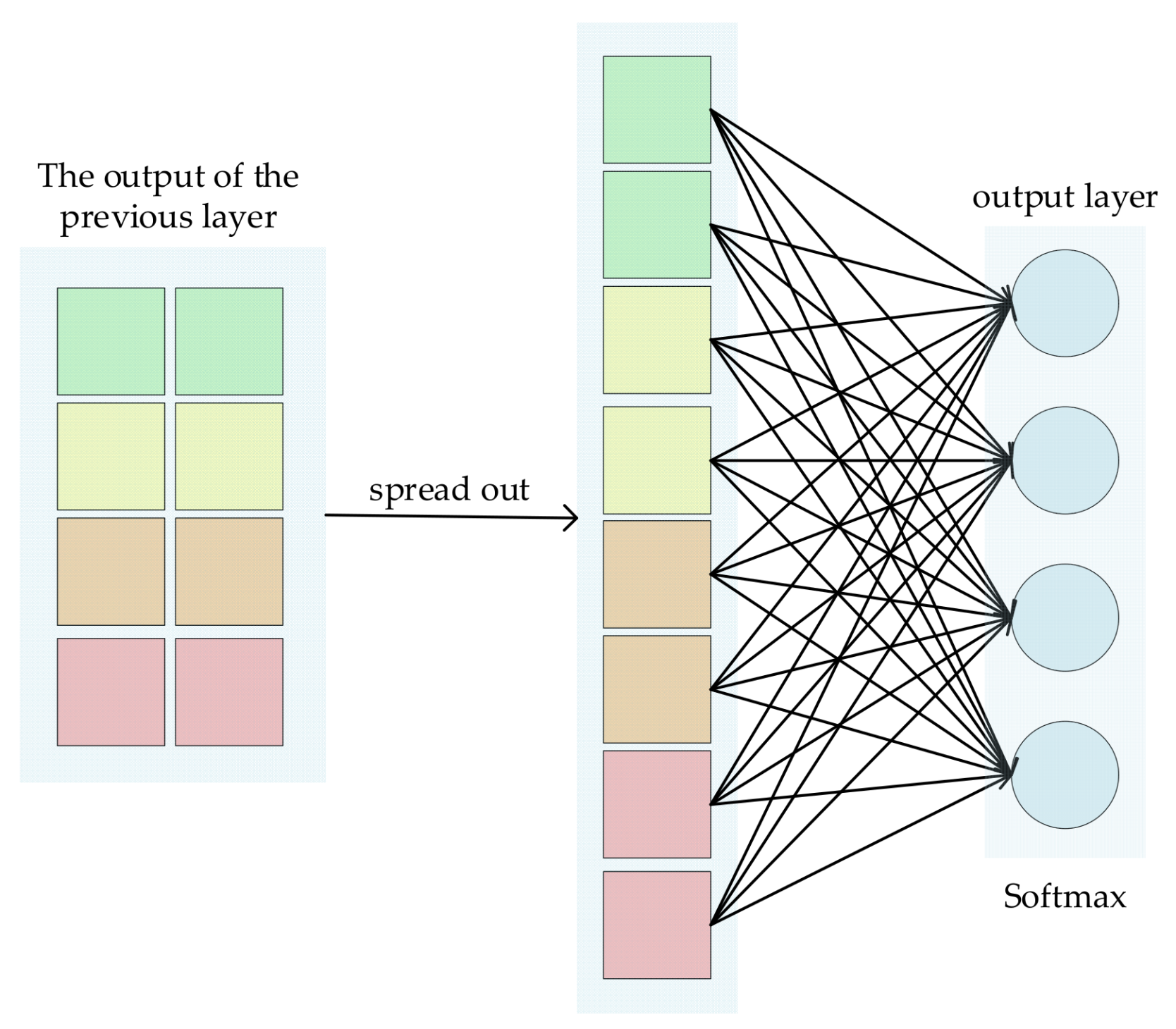
The full connection layer classifies the features that are extracted by the convolution kernel. To be specific, the output of the previous layer is first spread out as a one-dimensional vector (as shown in Figure 1), which is used as the input of the full connection layer, and the input and output are fully connected. The formula for the full connection layer is shown as
where represents the weighted value of the th neuron in the th layer and the th neuron in the layer, represents the logit value of the th output neuron at the layer, and represents the bias value of all neurons in the layer to the th neuron in the layer .
The Softmax function calculates the probability of all the classification tags, which is a multi-classification form that is obtained by logistic regression. It is often used in multi-classification problems. The specific expression is as follows
where represents the output value of the th neuron in the output layer and represents the sum number of categories.
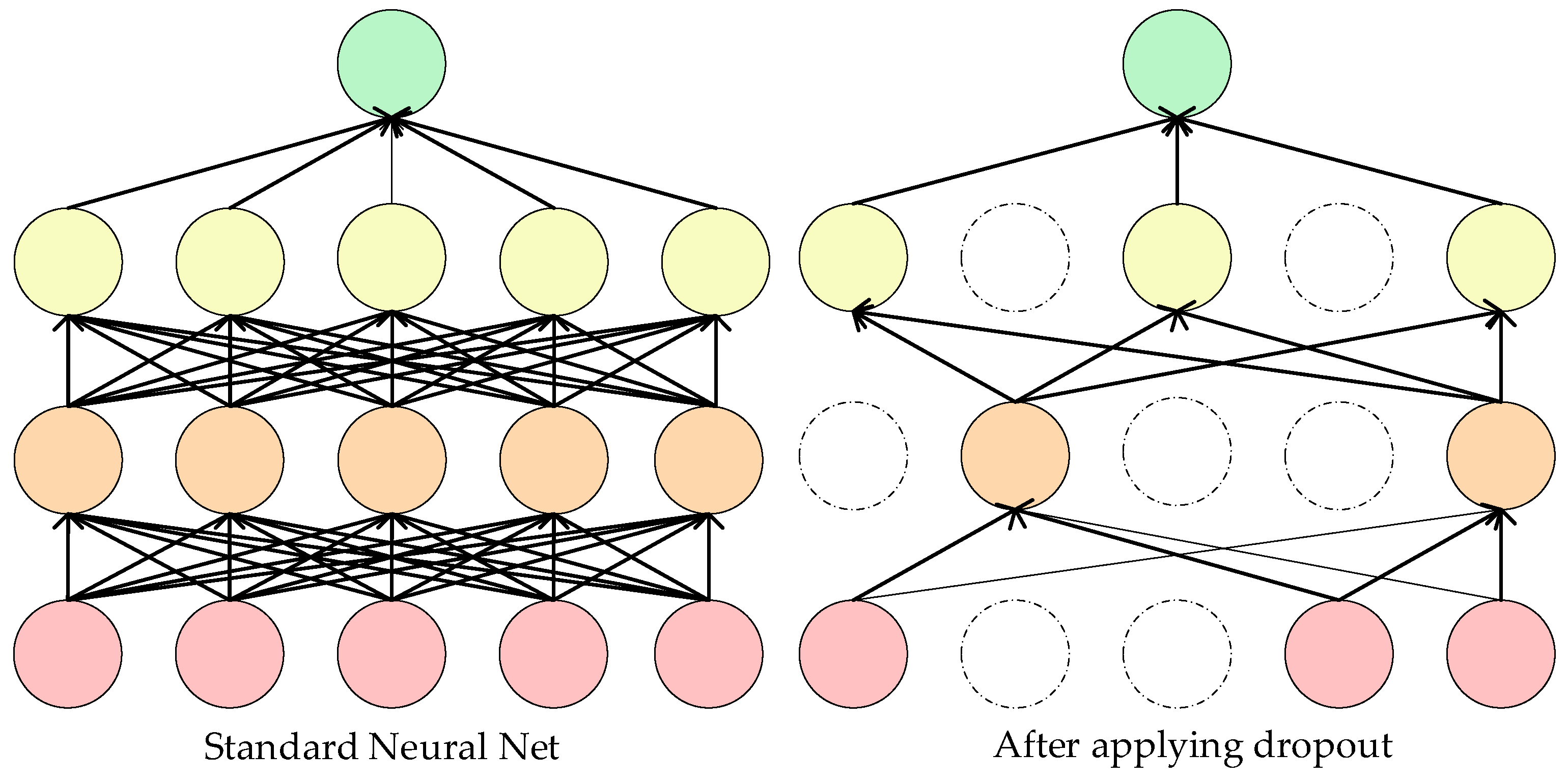
The dropout proposed by Hinton et al. [32] reduces the overfitting and enhances the generalization ability of a neural network. The dropout algorithm sets the neurons in a certain layer of the neural network to zero at a certain probability p, as shown in Figure 2. The algorithm weakens the joint adaptability of the same layer of neural nodes and improves the generalization ability. A neural network with N nodes is regarded as a set of models while using the Dropout algorithm. The number of training parameters is unchanged, and the optimal model is selected from the models as the best model by training.
2.2. Fault Diagnosis Process Based on 1D-CNN
The fault identification course of the rolling bearing that is based on the 1D-CNN is as follows.
- (1)
- A sensor is installed on the corresponding position of the rolling bearing.
- (2)
- The one-dimensional vibration signal is first collected as the raw data, and then the signal data is divided into training, validation, and test sets.
- (3)
- The training set is used as the input of 1D-CNN network. The model is trained, the validation set is used in order to verify the model performance, and appropriate network model parameters are selected.
- (4)
- The test set is put to the trained model, and the performance of the model is evaluated.
The 1D-CNN was evaluated while using the one-dimensional original vibration data set of the rolling bearing supplied by CWRU [33]. The dataset consists of 1000 samples, which are divided into the training set, validation set, and test set, according to the ratio of 6:2:2. Different loads were grouped into different fault categories, as shown in Table 1. The “0123 HP” in Table 1 represents a new bearing vibration data set that is composed of bearing vibration data sets, with loads of 0 HP, 1 HP, 2 HP, and 3 HP.
2.3. 1D-CNN Structure
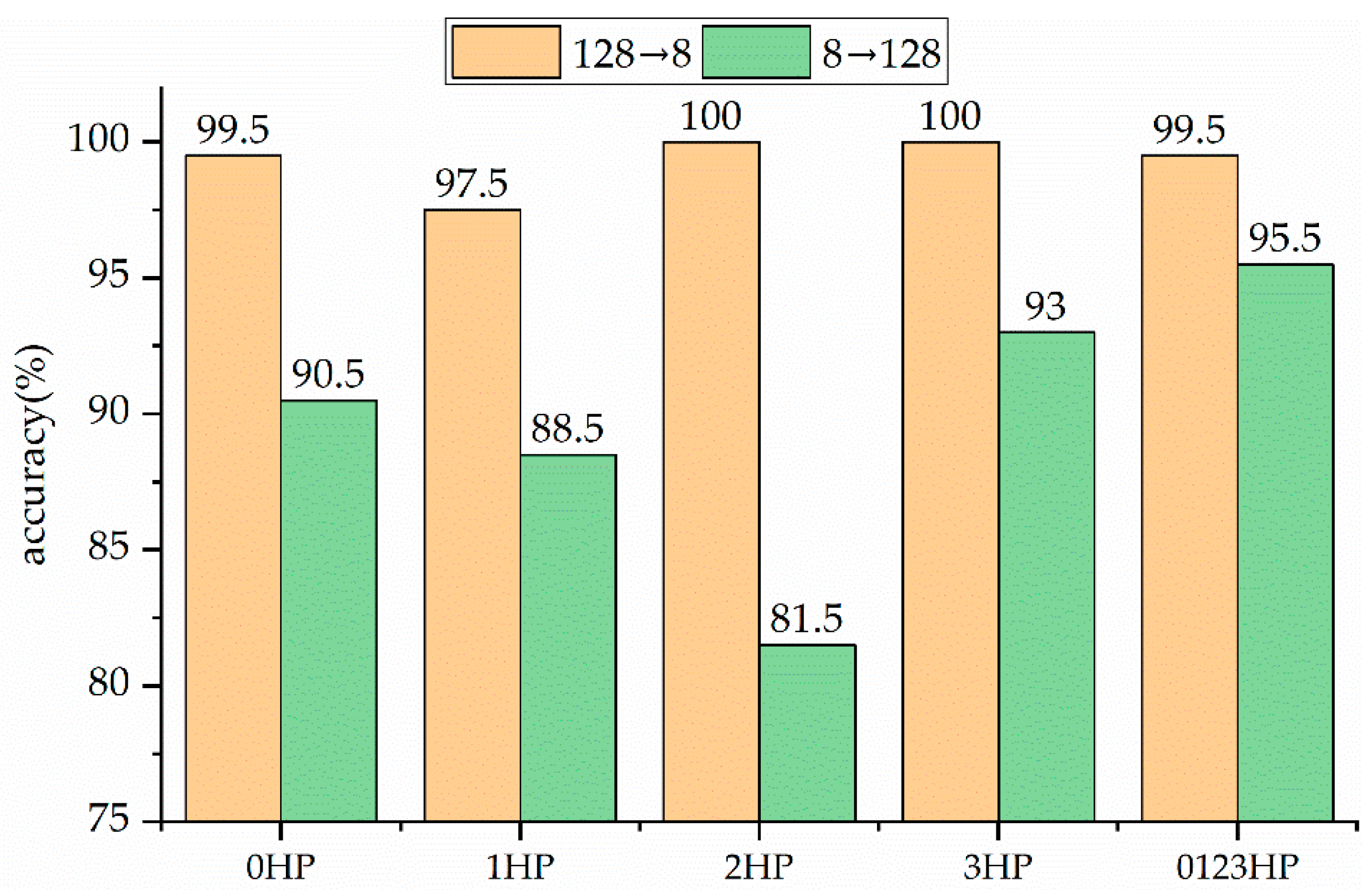
The number of convolution kernels in a convolutional neural network gradually increases with the reduction of the size of the convolution kernel, while the number of convolution kernels in the 1D-CNN model that is proposed in this paper also gradually decreases with the reduction of the size of the convolution kernel. The experimental results show that the 1D-CNN model has higher accuracy, with the number of convolution kernels decreasing with the size of the convolution kernel at different loads, as shown in Figure 3.
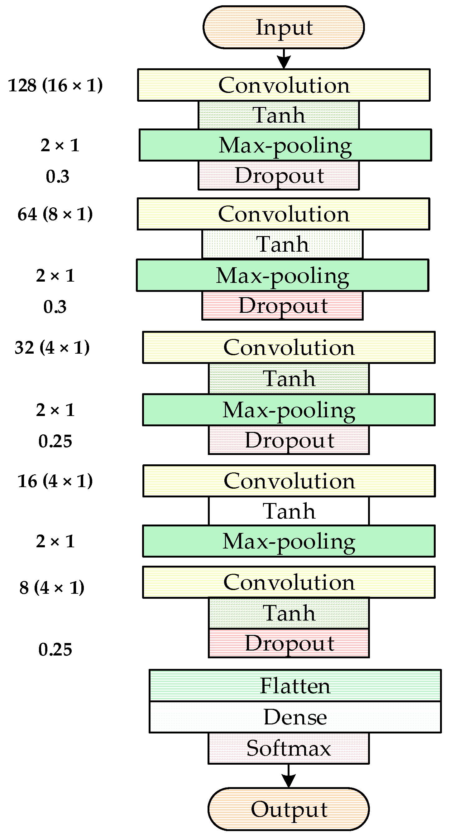
The 1D-CNN model structure and parameter setting in this paper are obtained through several experiments. The 1D-CNN structure incorporates five convolution layers, four pooling layers, and two full connection layers (Figure 4). Table 2 shows the specific detailed network structure parameters.
Step 1
In each convolution layer, the appropriate number and size of the convolution kernel performs one dimensional convolution operations. The input data are the one-dimensional signal that has a length of 1024. Five convolution layers use 128 convolution kernels of size 16 × 1 (Conv1), to Conv5), 64 of size 8 × 1 (Conv2), 32 of size 4 × 1 layer (Conv3), 16 of size 4 × 1 (Conv4), and eight of size 4 × 1 (Conv5). Tanh is the hyperbolic activation function for the five convolution layers.
Step 2
The pooling layer is appended to the Conv1, Conv2, Conv3, and Conv4, and carries out a 2 × 2 max-pooling operation. The dropout operation is executed after executing the first and second pooling layers and, then, the dropout ratio is set to 0.3. A dropout operation with a ratio of 0.25 is performed after the third pooling layer and that with a ratio of 0.25 after the fifth convolution layer. The dropout operation randomly selects and deletes neurons from the model in order to form a random subset of the neurons, solve the overfitting problem, and enhanced the generalization ability of the neural network model. This does not depend on connections between neurons that have specific connections. In the flatten layer, the extracted features from the five convolution layers are extended to a one-dimensional vector. The output layer contains 10 neurons. While using Softmax as the activation function, 10 types of faults are identified after training.
3. Data Set Description and Model Parameter Selection
3.1. Data Set Description
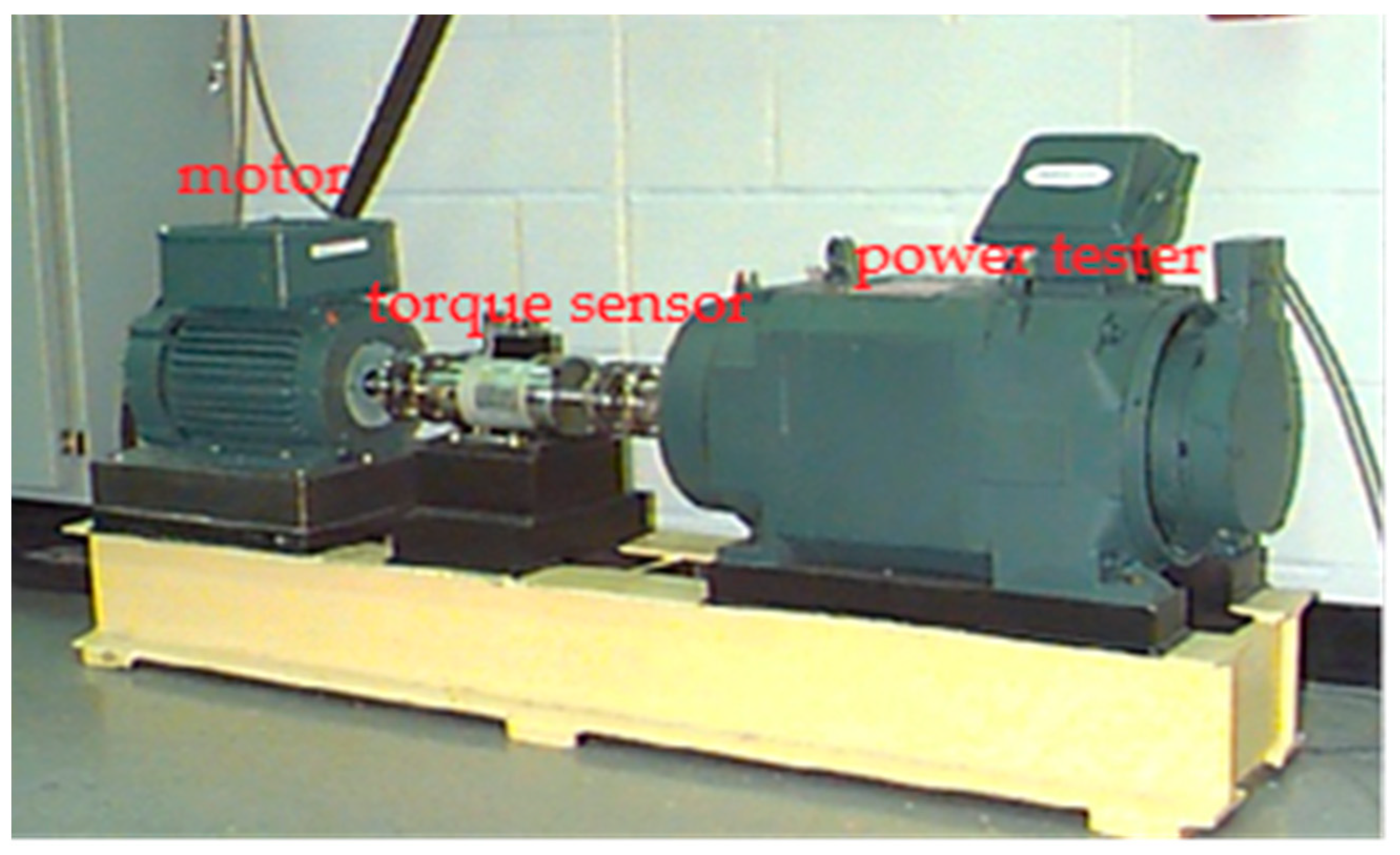
The 1D-CNN network model was programmed by Spyder in Anaconda3 (python3.7) while using Keras2.0.This 1D-CNN model was also tested on a computer that was equipped with 1.8 GHz quad-core i5-8265U, 8GB of RAM, and an NVIDIA MX250 graphics card. The CWRU data set is the benchmark data set and it is widely used in researches on diagnosing faults of the rolling bearing. The experimental platform was composed of a motor, torque sensor, power tester, and electronic controller, as indicated in Figure 5. Rolling bearings of Skf6205 and Skf6203 were used in the driving end and fan end of the experimental platform. Single-point damage was machined on the bearing by electric discharging machine (EDM). The diameter of the damage was 0.0028 mm, 0.0056 mm, 0.0083 mm, 0.011 mm and 0.0157 mm. The damage points of the bearing outer ring (fixed in operation) are set at 3 o’clock, 6 o’clock, and 12 o’clock, respectively, in order to make the collected fault data of the outer ring real and effective. The vibration acceleration signals of the rolling bearing are collected by acceleration sensors that are mounted on the fan end and the motor drive end housing. The sampling frequency of the fan end is 12 kHz, and the driver end is 12 kHz and 48 kHz. The bearing test platform uses 16-channel data recorders to the collected vibration signals and a torque sensor to the measured load and speed.
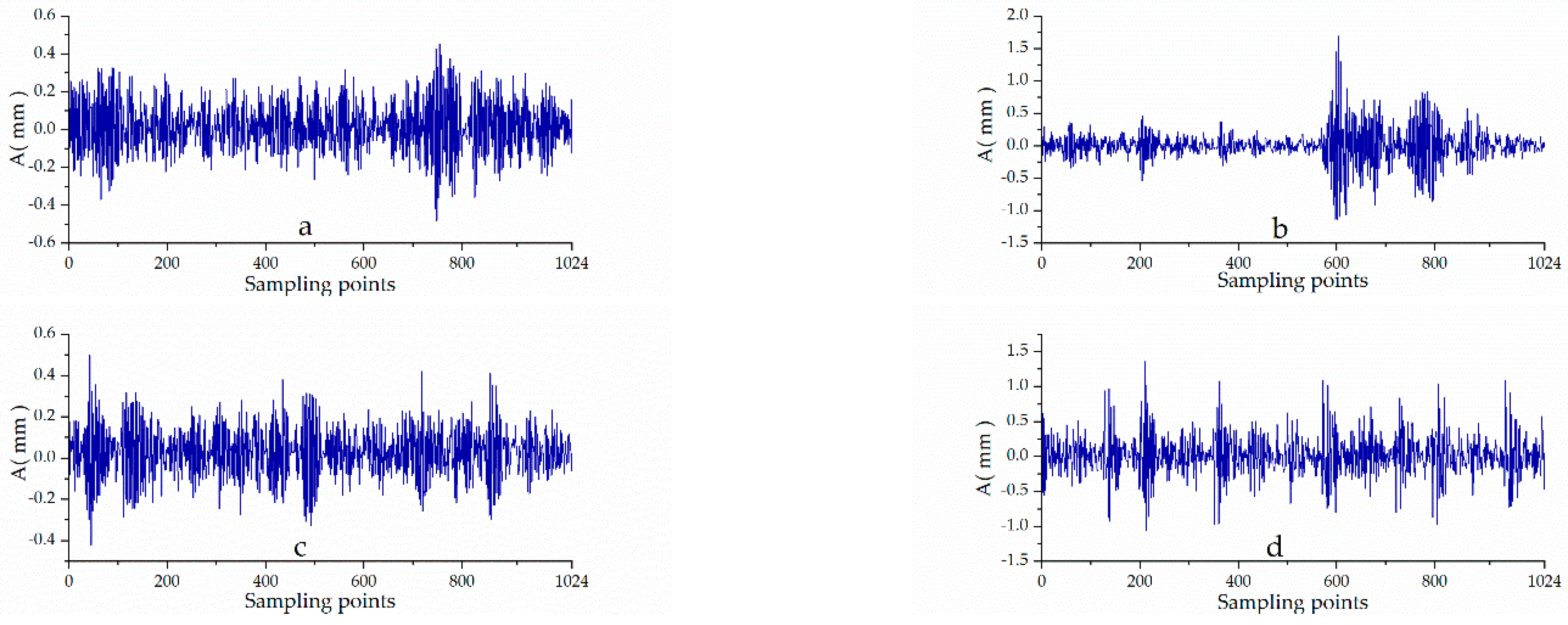
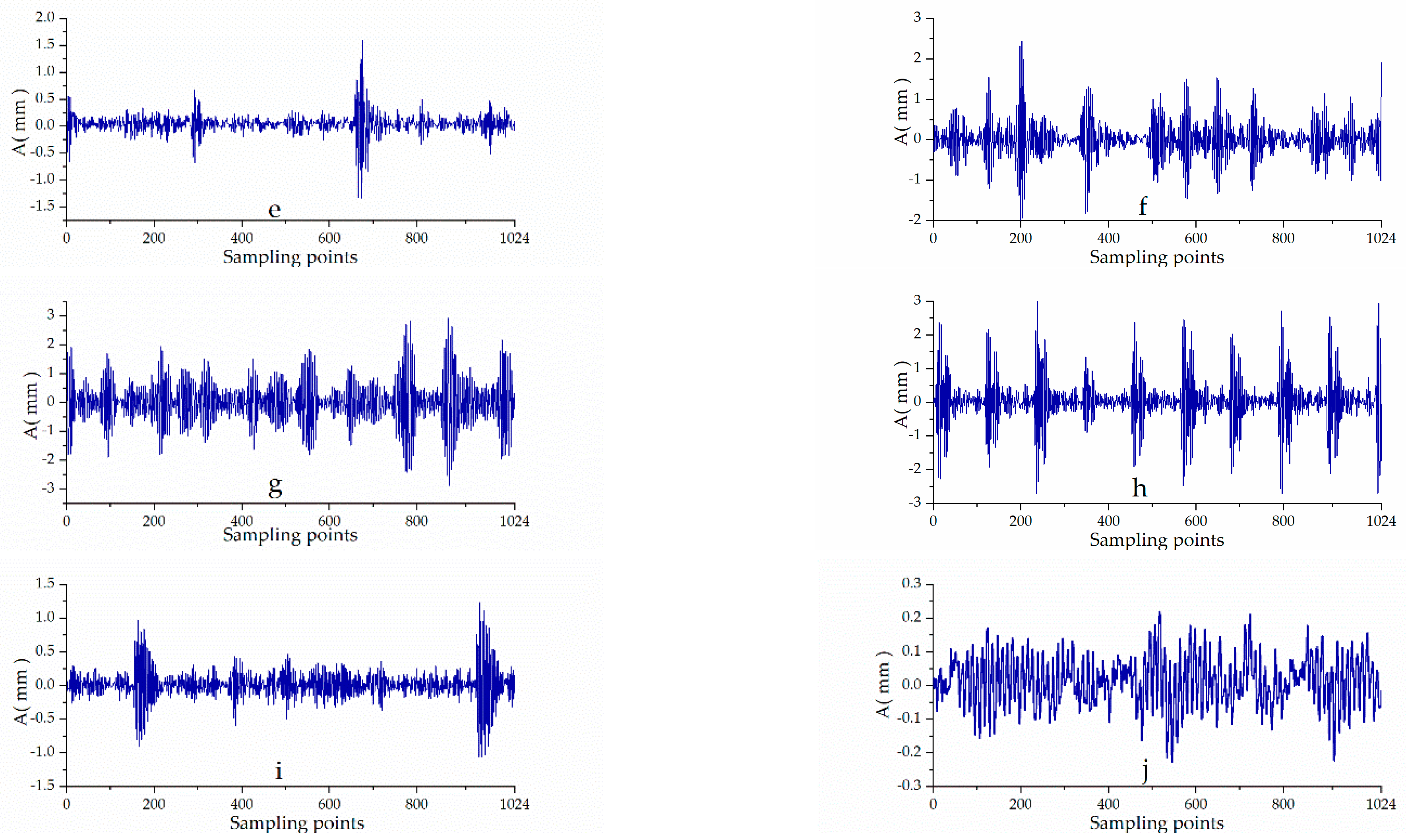
In the experiment, the vibration data from the acceleration sensor at the driving end were selected at 12 kHz sampling frequency. The data set included nine types of failures in the normal state of the bearing, the bearing inner ring, and the ball bearings at diameters of 0.0028 mm, 0.0056 mm, and 0.0083 mm. The damage points of the bearing’s outer ring were in the direction of3, 6, and 12 o’clock. The vibration signals of the 10 fault types were selected when the load was 0 HP, 1 HP, 2 HP and 3HP with 1024 data points (the motor speed is 1797/min. At the sampling frequency of 12 kHz, there are 60/1797 × 12000 = 400.67 sampling points in each cycle. The sample length is set to 1024, which can contain sample data of 1024/400 = 2.56 cycles, so as to ensure that each sample contains abundant fault feature information). Different fault types under different loads are divided into the training set, validation set, and test set according to the ratio of 6:2:2. Table 1 shows the data set of rolling bearing vibration signals. Figure 6 reveals the original vibration signals of the 10 fault types under 0 HP.
3.2. 1D-CNN Model Parameter Selection
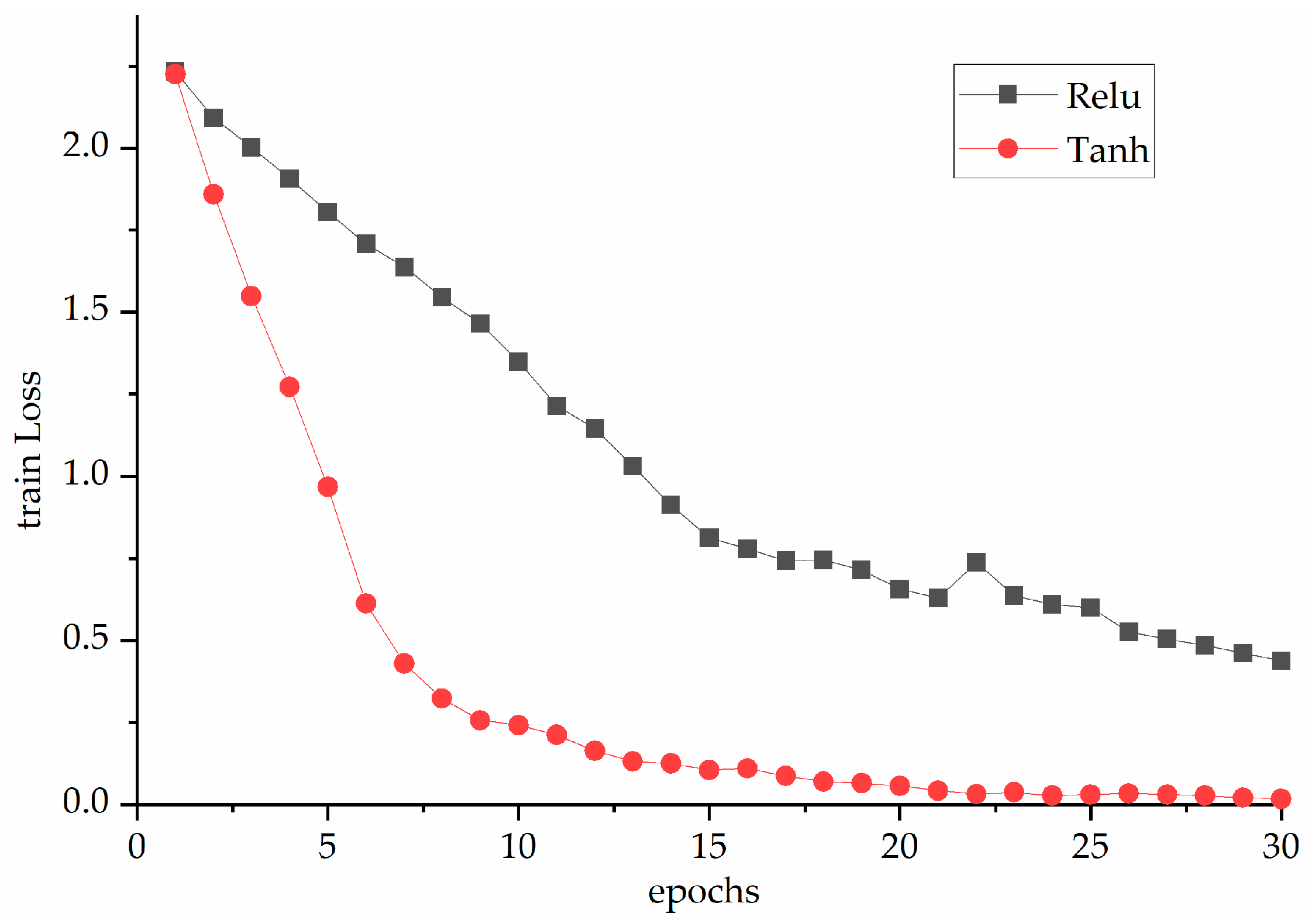
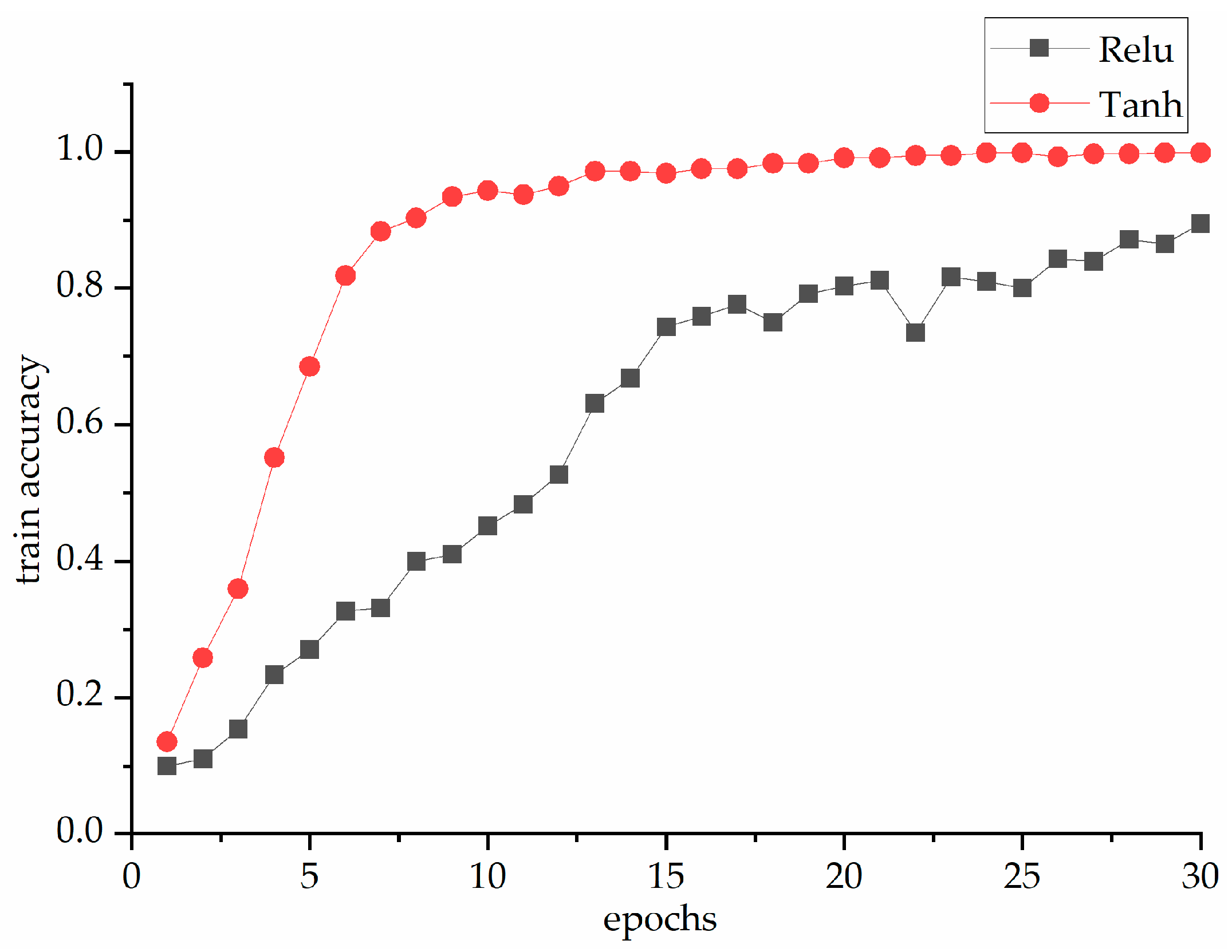
The neural network is a multilayer compound function in mathematics. If there is no activation function, then the neural network will be a linear function. However, samples are not always linearly separable, so the activation function with nonlinear factors, such as Tanh and Relu, should be used in order to solve problems that cannot be settled. Relu makes the output of neurons with a negative input value zero, which reduces the interdependence among parameters and speeds up the calculation. In order to explore the influence of Tanh and Relu on the 1D-CNN network, their activation functions are used in the experiment under the load of 0HP. Figure 7 and Figure 8 show the curve of loss function and accuracy in the training process.
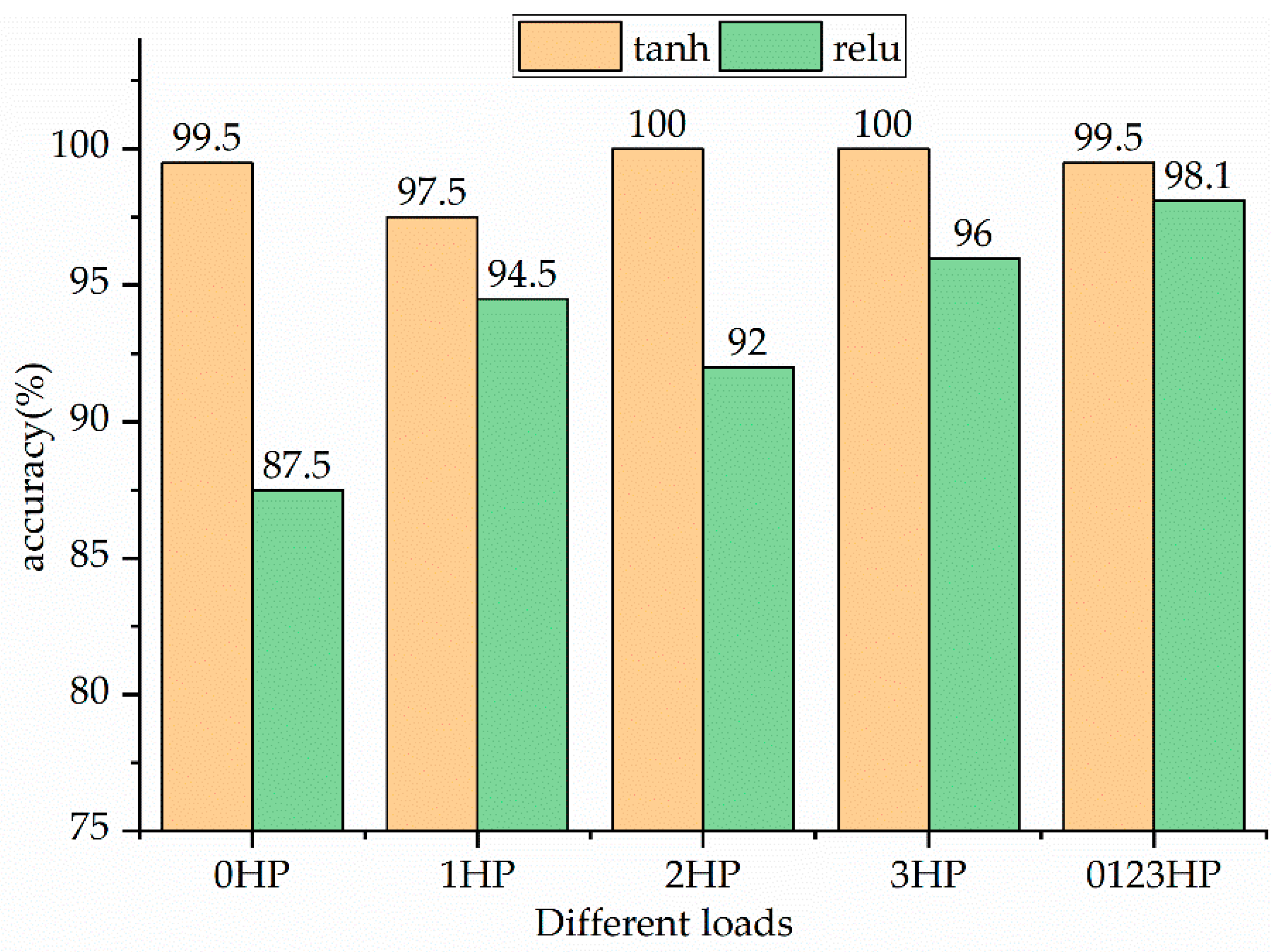
In Figure 7, the loss curve can be seen in the process of 30 finite iterations, despite the fact that the loss function values of both are constantly decreasing. However, if the activation function is Tanh, then the curve converges at a significantly faster rate and, finally, approaches zero value. In contrast, if the activation function is Relu, then the convergence becomes slower. The accuracy curve depicted in Figure 8 shows that, with the increase of iteration times, the activation function uses Tanh in order to converge faster and more accurately than Relu. In order to further prove the necessity of selecting Tanh as the activation function, experiments were carried out at 0 HP, 1 HP, 2 HP, 3 HP, and 0123 HP. The experimental results that are shown in Figure 9 indicate that Tanh is more accurate than Relu if the former is selected as the activation function for the 1D-CNN network model proposed in this paper. According to the corresponding experimental results, Relu was deemed to be unsuitable for the 1D-CNN model that was proposed in this paper.
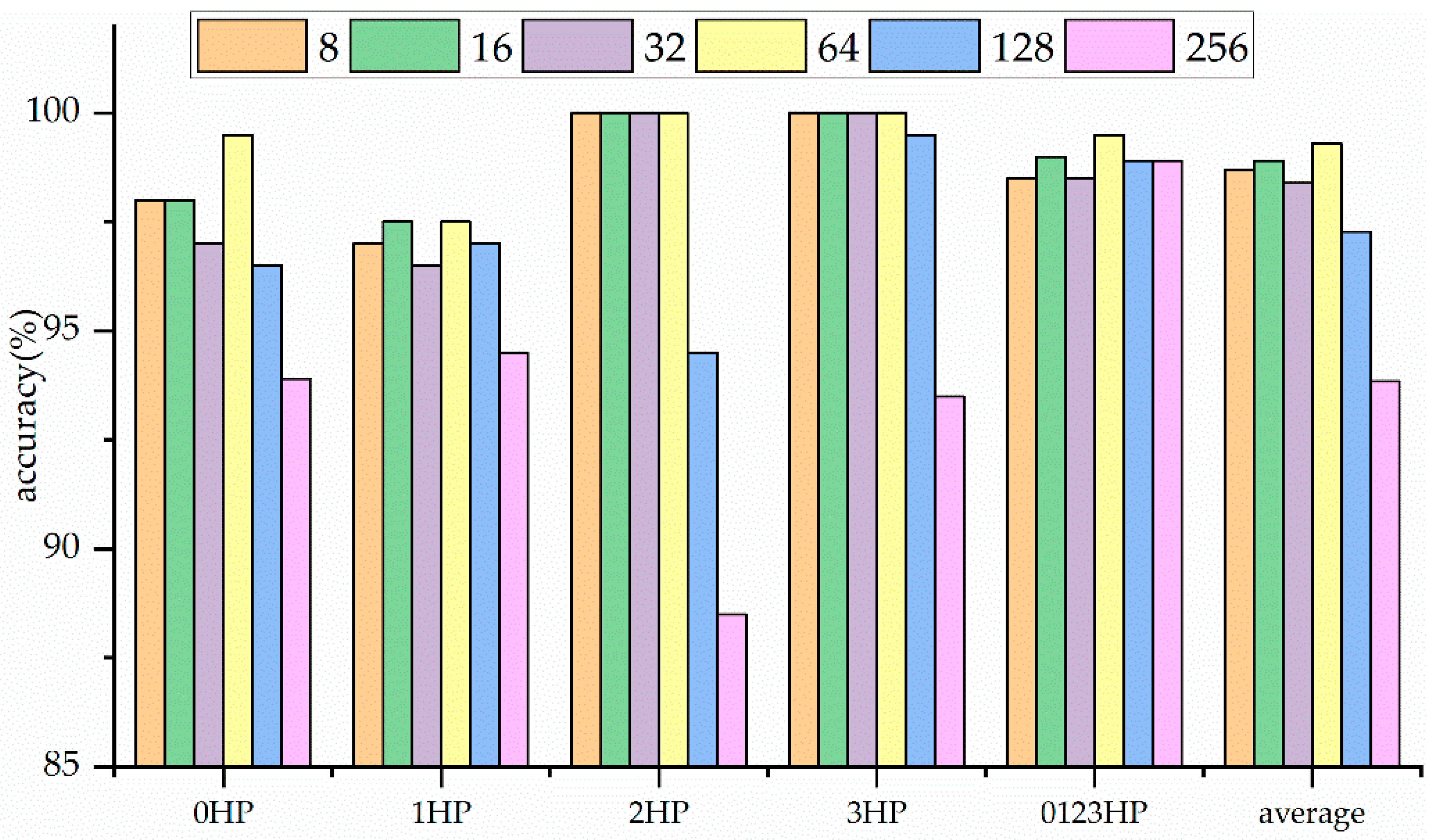
When training the network model, a batch size impacts not only the training speed, but also the accuracy. A large batch-size can expedite the training process, but it requires a large memory space in a computer. For small batch-size in the training process, although the operation speed is slower and some noise is produced, the appearance of noise is also helpful in preventing the training process from falling into local optimal. Therefore, it is very important to select an appropriate batch-size. In this paper, six different batch-sizes (8, 16, 32, 64, 128 and 256) were selected for comparison test under different loads. The experimental results, as shown in Figure 10, indicate that, when the batch-size is 8, 16, 32 and 64, the average accuracy of the 1D-CNN model on different loads reaches more than 98%, while the batch size is 128, 256, the average accuracy of different loads reads 97.28% and 93.86%, respectively. The experimental results show that the 1D-CNN model has the highest average accuracy of 99.3% under different loads when the batch size is 64.
3.3. The Specific Parameters of Six Models
The 1D-CNN model is compared with the experiments of five different models that are based on machine learning and deep learning, so as to prove the effectiveness of the 1D-CNN model in the fault diagnosis of rolling bearings. The five models are LSTM (Long-Short Term Memory), MLP, SVM, Random forest, and KNN. The datasets shown in Table 1 were used by the six models. The specific parameters of LSTM and MLP network models are selected after experiments are done with the same selection method as the parameters of 1D-CNN. GridSearchCV (10-fold cross verification parameters) is used in order to select several parameters that affect the performance of SVM, RandomForest, and KNN models. Experiments were carried out under loads of 0 HP, 1 HP, 2 HP, 3 HP, and 0123 HP (represents a new bearing vibration data set that is composed of bearing vibration data sets with loads of 0 HP, 1 HP, 2 HP, and 3 HP). The parameters of each model are as follows:
- (1)
- 1D-CNN modelThe learning ratio was set to 0.001 and the activation function is set to Tanh. The optimizer was Adam, which combines the advantages of Adagrad and RMSprop algorithm and it has high computing efficiency and low memory requirement. The loss function is categorical_crossentrop, the batch-size was set to 64, and the iteration time was 30.
- (2)
- LSTM modelThe first layer of the LSTM had 32 neurons with Tanh as the activation function. The second layer had 32 neurons in the full connection layer with Relu as the activation function. The third layer had 10 neurons and it was classified by Softmax. The learning ratio was set to 0.001 and the optimizer is Adam. The loss function was categorical_crossentropy. The batch- size was 32 and iteration time was 30.
- (3)
- MLP modelThe first, second, third, and fourth layers were the whole connective layer with 300, 400, 200 and 100 neurons, respectively. The activation function was Relu. Dropout operations were adopted with a probability of 0.4 in each full connection layer. The fifth layer was the output layer with 10 neurons and it was classified by Softmax. The learning ratio was set to 0.002 and the optimizer is Adam. The loss function wascategorical_crossentropy. The batch- size was 32 and the iteration time was 40.
- (4)
- SVM modelThe GridSearchCV (10-fold cross verification parameters) is adopted. Gaussian kernel (RBF) is selected as the kernel function of SVM. The penalty factor C is determined to be 128, and gamma (controls the width of gaussian kernel and it determines the distribution of data mapped to the new feature space) is 0.002.
- (5)
- RandomForest modelThe GridSearchCV (10-fold cross verification parameters) is adopted. Three-hundred decision trees were used in order to construct the random forest model. The maximum depth of the random forest tree is 16, and the minimum number of tree splits was 5.
- (6)
- KNN modelThe GridSearchCV (10-fold cross verification parameters) is used for the KNN model in order to determine the best K value of 1.
4. Experimental Results and Analysis
4.1. Compared with Other Model Experiments
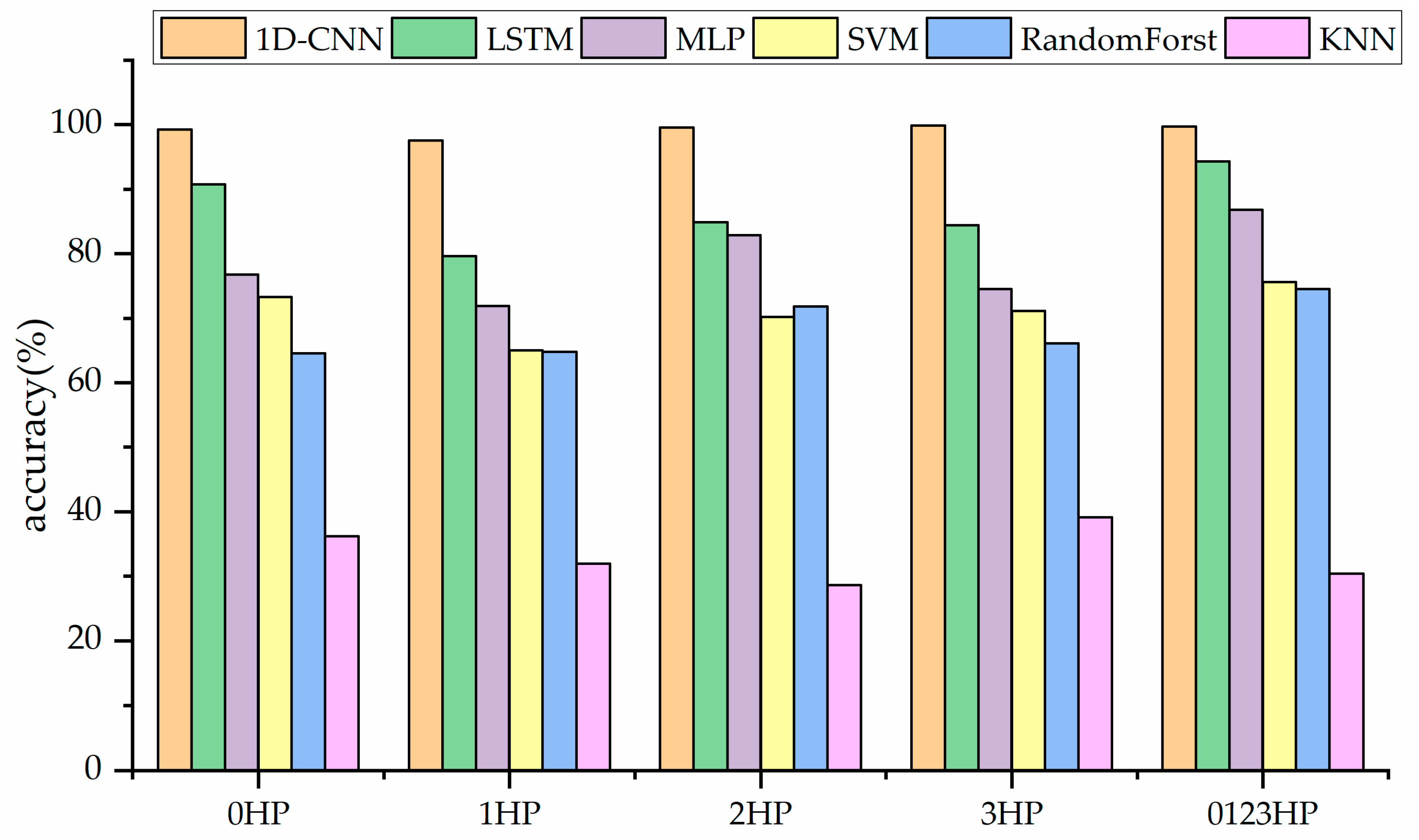
Each model is cross-validated with 10-fold when tested on different loads in order to better evaluate the performance of the model. The experimental results of various rolling bearing fault diagnosis methods are shown in Table 3 and Table 4, and Figure 10. Table 3 shows the accuracies of the six models under different loads and the average accuracy of the 1D-CNN network in different loads is99.2%.The 1D-CNN’s average accuracy is 65.94%, 30.82%, and 28.15% higher than KNN, RandomForest, and SVM, respectively. As the results show, these three bearing failure methods that are based on machine learning perform worse than the 1D-CNN network proposed in this paper, and the main causes are as follows: when we use KNN algorithm, the data should be preprocessed to some extent; SVM does not perform well in data sets with many feature points; RandomForst sensitive to noise easily leads to overfitting.
The average accuracy of the 1D-CNN is 12.41% and 20.61% higher than that of LSTM and MLP. The average accuracies of LSTM (86.79%) and MLP (78.59%)are higher than RandomForst (68.38%), KNN (33.26%),and SVM (71.05%).From the experimental results, the deep learning method is superior to machine learning, mainly because machine learning cannot learn some nonlinear relations in complex bearing vibration signals well, while deep learning method has great advantages in analyzing complex and non-stationary signals. In the experiment, these six methods were tested on the loads of 0 HP, 1 HP, 2 HP, 3 HP, and 0123 HP, while the 1D-CNN model achieved high accuracy on each load, with the difference between the highest accuracy and the lowest accuracy only being 2.3%.
Table 4 and Figure 11 show the average accuracies of different models under different loads. The 1D-CNNhad the accuracies of 99.3%, 97.6%, 99.5%, 99.9%, and 99.68% under different loads, with an average accuracy of 99.2%, which was higher than those of the other five models. Moreover, the standard deviation of the 1D-CNN was only 0.82%, which is lower than the 5.17%, 5.50%, 3.56%, 4.08%, and 3.89% of the other five methods. These results prove the effectiveness of the 1D-CNN in fault diagnosis under different loads.
4.2. Performances under Different Loads
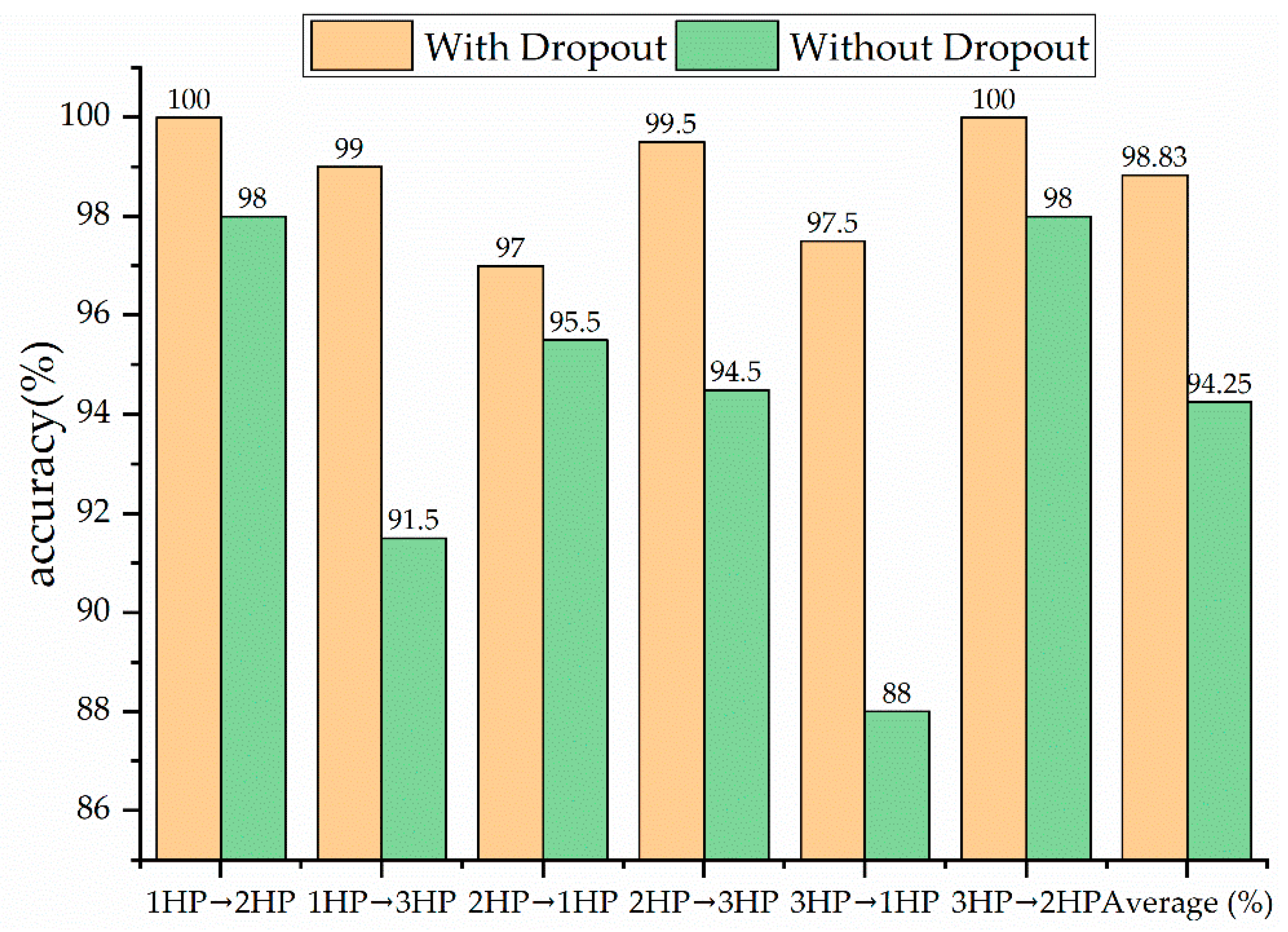
The Dropout layer is added to 1D-CNN network model in order to avoid overfitting and enhance the generalization ability of 1D-CNN network model. The experimental results that are shown in Figure 11 prove that 1D-CNN can achieve higher accuracy in cross-load training
Cross-load training was carried out under the three loads of 1 HP, 2 HP, and 3 HP, as shown in Figure 12. The experimental results show that the generalization ability of the 1D-CNN network model is significantly improved with the addition of Dropout layer; especially, the model accuracy is increased by 9.5% under the condition of 3 HP→1 HP. The average accuracy of cross-load training increased from 94.25% (without Dropout) to 98.83% (with Dropout) (“3 HP→1 HP” means training at 3 HP and testing at 1 HP).
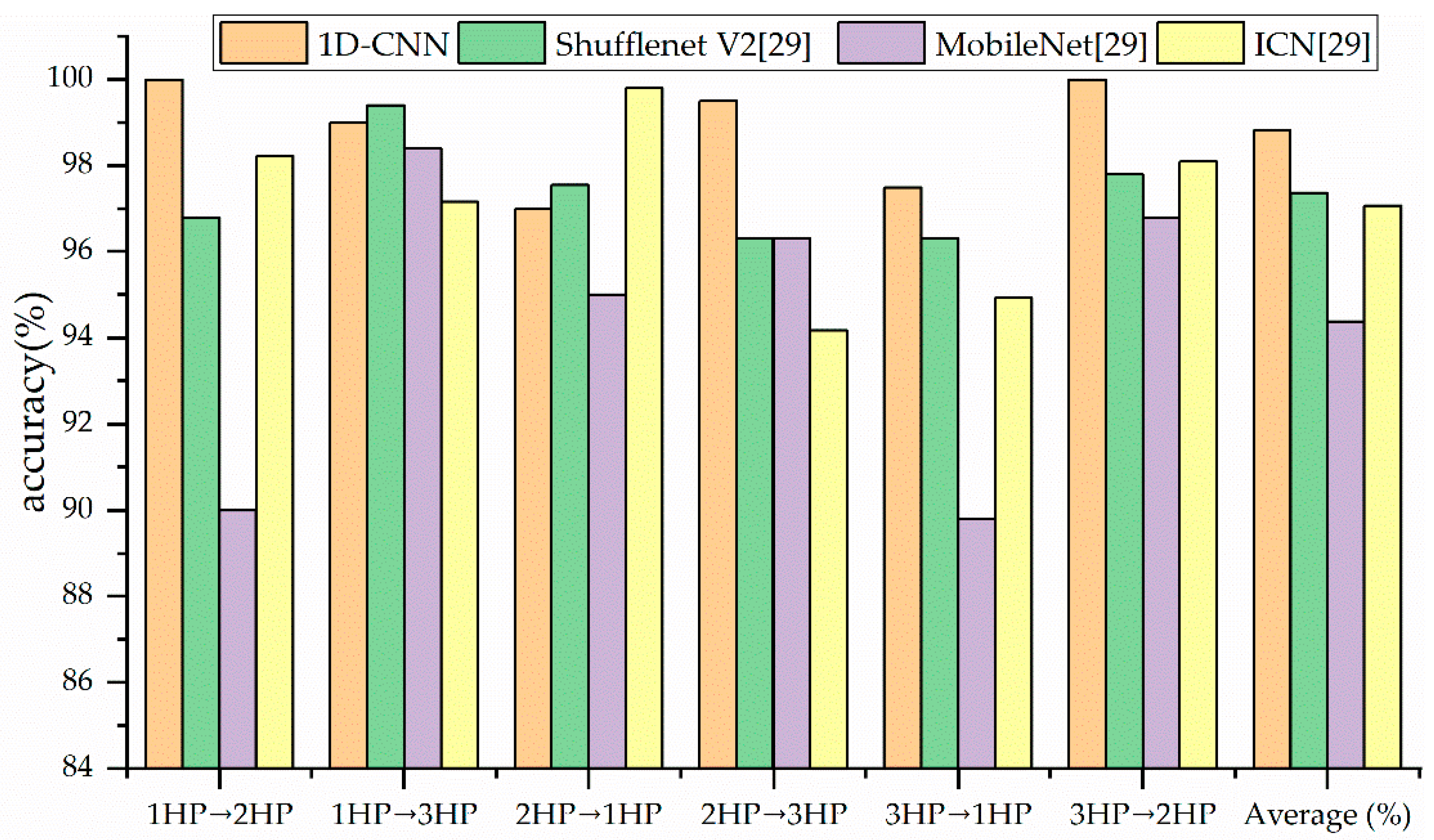
In the practical application, the fault samples of equipment under various loads are difficult to collect. Thus, the faults of rolling bearings are collected under a certain load. However, training the model for diagnosing the faults requires the fault data under different loads. In the research of this paper, the generalization ability of the 1D-CNN under different loads was investigated and the result was compared to that of Shufflenet V2, MobileNet, ICN [34], DFCNN [35], and PFC-CNN [36]. Table 5 and Figure 13 show the specific experimental contrast results (“1 HP→2 HP” means using 1HP as a training set and 2 HP as a test set).
Table 5 shows that the highest and lowest accuracy of the 1D-CNN is 100% and 97%. The lowest accuracy was lower than that of Shufflenet V2 (96.3%) and ICN (94.17%). The average accuracy was 98.3%, which was higher than that of Shufflenet V2 (97.36%), MobileNet (94.38%), ICN (97.07%), DFCNN (90.05%), and PFC-CNN (93.31%). The results validate that the 1D-CNN is effective in diagnosing the bearing faults under different loads.
Figure 13 shows the accuracies of the diagnosis under various loads with different methods. Except for the case of 2HP→1HP, the 1D-CNN model had higher accuracies than Shufflenet V2 and ICN. In other cases, the proposed model showed effectiveness in diagnosing the faults under cross-loads.
4.3. Visual Analysis of Validity of 1D-CNN Model
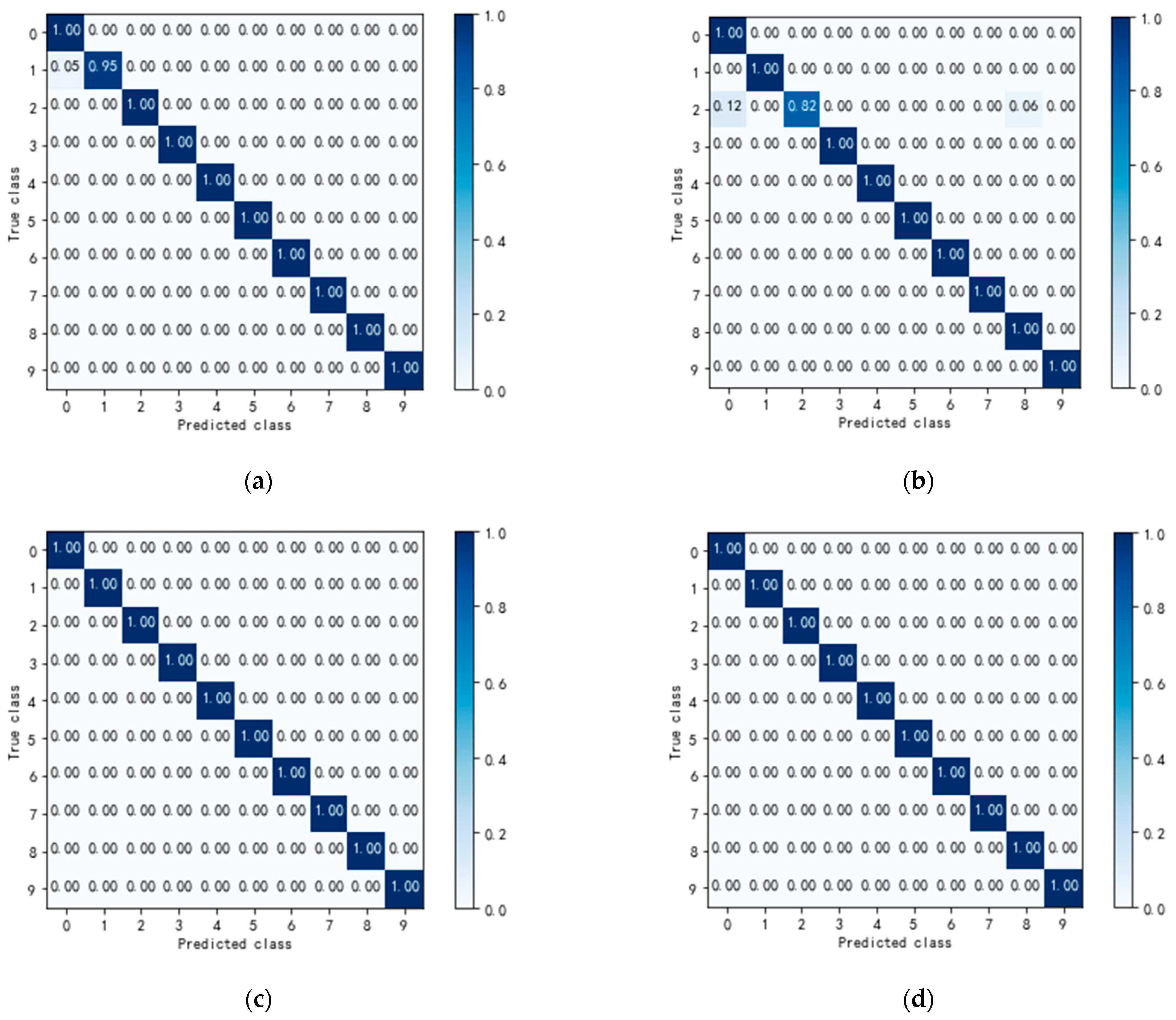
The results under different loads are summarized in the confusion matrix in order to more intuitively assess the accuracy of the 1D-CNN model bearing fault diagnosis. Table 6 shows the bearing status that is represented by each number in Figure 14. The confusion matrix presents the predicted result of the samples on the horizontal axis and the actual label of the samples on the vertical axis. 5% of the ball fault (0.0056 mm) were incorrectly predicted as the ball fault (0.0028 mm) under 0 HP and 12% of the ball fault (0.0084 mm) were incorrectly predicted as ball fault (0.0028 mm) under 1HP.Under the load of 0 and 1 HP, errors appeared in the diagnosis and prediction of the ball fault, as noise masks the characteristic information of the ball fault under lower loads. In other cases, the 1D-CNN has an appropriate prediction.
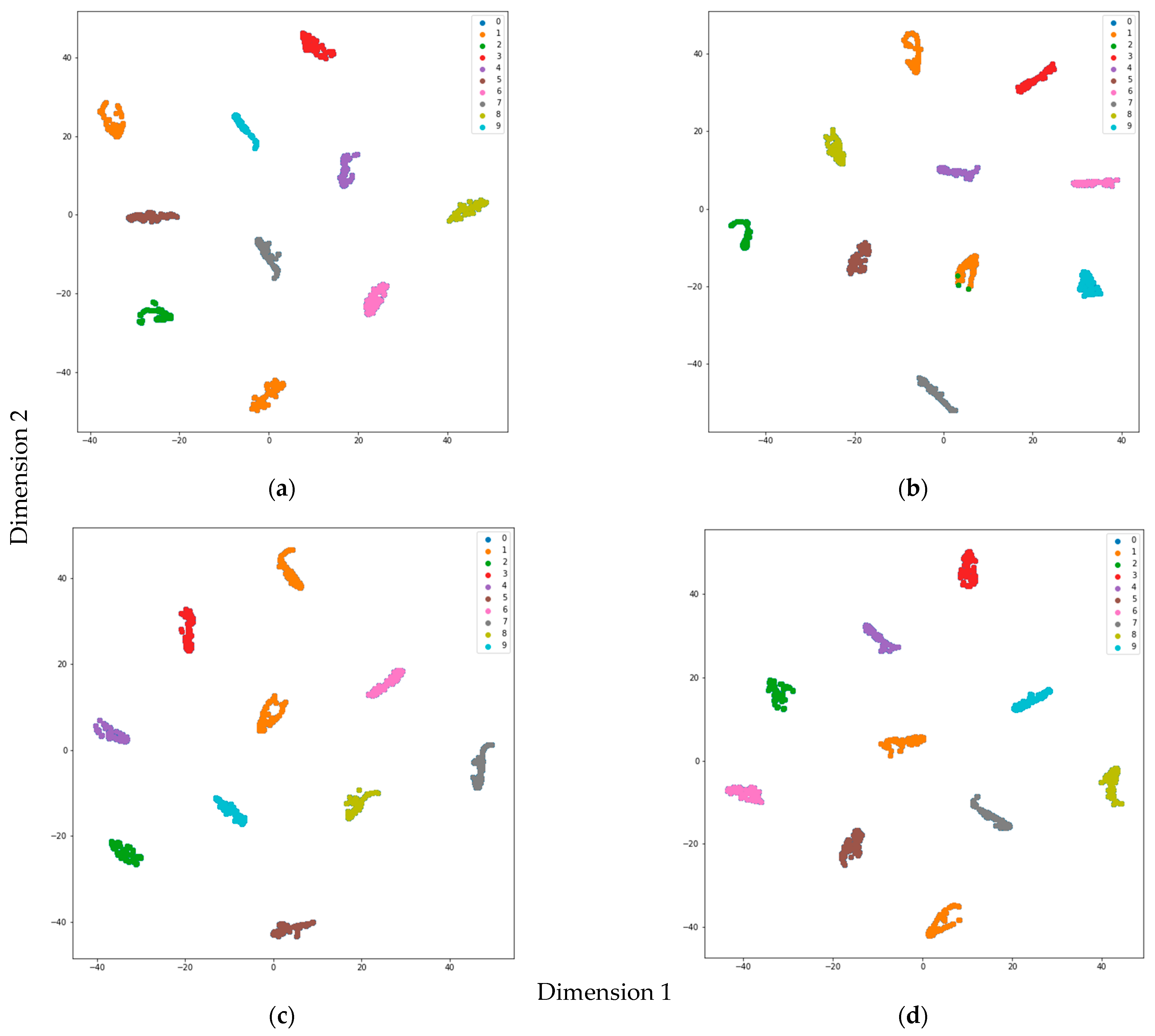
t-SNE is a dimension reduction algorithm that is based on manifold learning, which is different from the traditional PCA (Principal Component Analysis) and LDA (Linear Discriminant Analysis) methods. t-SNE uses normalized Gauss collated high-dimensional spatial data features for similarity modeling. At the same time, t-distribution is used in order to model the similarity of low-dimensional spatial data. KL distance narrows the distance distribution of high- and low-dimensional space and allows for visualizing high-dimensional data into two-dimensional or three-dimensional graphics. The t- SNE visualization algorithm is used in order to prove that the 1D-CNN distinguishes different fault types (Figure 15). By reducing the data’s dimension in the prediction of results under different loads [37], the t-SNE algorithm visualizes the prediction results of different loads in the CWRU data set. Table 6 shows the status of the bearings that are represented by the numbers; Figure 15 shows that the bearing failure characteristics representing the alike fault type are gathered together, and various types of bearing faults are separated, which shows that the 1D-CNN effectively distinguishes fault characteristics under different loads.
5. Conclusions
A new method for diagnosing faults of the rolling bearingis proposed using a 1D-CNN. The vibration dataset of the rolling bearing supplied by Case Western Reserve University (CWRU) is used in order to verify the model. The following conclusions can be drawn from a series of experiments in this paper.
- (1)
- The method that is proposed in this paper shows an average accuracy of 99.2% under a single load and 98.83% across different loads. Moreover, the original vibration data of the bearings are directly used without preprocessing.
- (2)
- In this paper, we propose a 1D-CNN network structure, in which the number of convolution kernels decreases with the reduction of the size of the convolution kernel, and that network structure effectively improves the accuracy of bearing fault diagnosis.
- (3)
- The 1D-CNN model has great advantages for analyzing complex and non-stationary signals when compared with traditional machine learning methods.
- (4)
- The Dropout layer added to the 1D-CNN model effectively improves the accuracy of cross-load training and it enhances the generalization ability of the model.
In the actual industrial environment, the vibration data of the bearing will be disturbed by great noise, and the vibration data of the rolling bearing will be increasingly complicated. In future research, with a view to better integrating deep learning and fault diagnosis, we will continue exploring how to accurately diagnose bearing faults in complex bearing vibration data with noise.
Author Contributions
Data curation, C.-C.C.; Formal analysis, C.-C.C.; Funding acquisition, C.-C.C.; Investigation, C.-C.C.; Methodology, C.-C.C.; Project administration, C.-C.C., G.Y., C.-C.W. and Q.Y.; Resources, C.-C.C., G.Y. and C.-C.W.; Software, Z.L. and C.-C.W.; Supervision, Z.L., G.Y. and C.-C.W.; Validation, Z.L.; Visualization, Z.L. and G.Y.; Writing—original draft, Z.L. All authors have read and agreed to the published version of the manuscript.
Funding
The work was partially supported by the National Key Scientific Research Program of China under Grant No. 2018YFC1406603, the National Science Council of Taiwan under grant MOST 107-2221-E-507-002-MY3, the Training Program of Fujian Excellent Talents in University, and the Open Project Fund of Fujian Shipping Research Institute.
Institutional Review Board Statement
Not applicable.
Informed Consent Statement
Not applicable.
Data Availability Statement
We include a data availability statement with all Research Articles published in an MDPI journal. The nature of the data in an mat file, and the data can be accessed on the website: https://csegroups.case.edu/bearingdatacenter/home, there are no restrictions on data access. The data used to support the findings of this study are included in the article.
Conflicts of Interest
The authors declare no conflict of interest. The funders had no role in the design of the study; in the collection, analyses, or interpretation of data; in the writing of the manuscript, or in the decision to publish the results.
References
- Nandi, S.; Toliyat, H.A.; Li, X. Condition Monitoring and Fault Diagnosis of Electrical Motors—A Review. IEEE Trans. Energy Convers. 2005, 20, 719–729. [Google Scholar] [CrossRef]
- Lei, Y.; Lin, J.; Zuo, M.J.; He, Z. Condition monitoring and fault diagnosis of planetary gearboxes: A review. Measurement 2014, 48, 292–305. [Google Scholar] [CrossRef]
- Fan, L.; Wang, S.; Wang, X.; Han, F.; Lyu, H. Nonlinear dynamic modeling of a helicopter planetary gear train for carrier plate crack fault diagnosis. Chin. J. Aeronaut. 2016, 29, 675–687. [Google Scholar] [CrossRef] [Green Version]
- Gao, Z.; Cecati, C.; Ding, S.X. A Survey of Fault Diagnosis and Fault-Tolerant Techniques—Part I: Fault Diagnosis With Model-Based and Signal-Based Approaches. IEEE Trans. Ind. Electron. 2015, 62, 3757–3767. [Google Scholar] [CrossRef] [Green Version]
- Li, D.Z.; Wang, W.; Ismail, F. An Enhanced Bispectrum Technique with Auxiliary Frequency Injection for Induction Motor Health Condition Monitoring. IEEE Trans. Ind. Electron. 2015, 64, 2679–2687. [Google Scholar] [CrossRef]
- Filippetti, F.; Bellini, A.; Capolino, G. Condition monitoring and diagnosis of rotor faults in induction machines: State of art and future perspectives. In Proceedings of the 2013 IEEE Workshop on Electrical Machines Design, Control and Diagnosis (WEMDCD), Paris, France, 11–12 March 2013; pp. 196–209. [Google Scholar]
- Kral, C.; Habetler, T.G.; Harley, R.G. Detection of mechanical imbalances of induction machines without spectral analysis of time-domain signals. IEEE Trans. Ind. Appl. 2004, 40, 1101–1106. [Google Scholar] [CrossRef]
- Zhang, X.; Liu, Z.; Wang, J.; Wang, J. Time–frequency analysis for bearing fault diagnosis using multiple Q-factor Gabor wavelets. ISA Trans. 2019, 87, 225–234. [Google Scholar] [CrossRef]
- Gao, H.; Liang, L.; Chen, X.; Xu, G. Feature extraction and recognition for rolling element bearing fault utilizing short-time Fourier transform and non-negative matrix factorization. Chin. J. Mech. Eng. 2015, 28, 96–105. [Google Scholar] [CrossRef]
- Li, Y.; Xu, M.; Huang, W.; Zuo, M.J.; Liu, L. An improved EMD method for fault diagnosis of rolling bearing. In Proceedings of the 2016 Prognostics and System Health Management Conference (PHM-Chengdu), Chengdu, China, 19–21 October 2016; pp. 1–5. [Google Scholar]
- Li, H.; Liu, T.; Wu, X.; Chen, Q. Research on bearing fault feature extraction based on singular value decomposition and optimized frequency band entropy. Mech. Syst. Signal Process. 2019, 118, 477–502. [Google Scholar] [CrossRef]
- Battineni, G.; Sagaro, G.G.; Chinatalapudi, N.; Amenta, F. Applications of Machine Learning Predictive Models in the Chronic Disease Diagnosis. JPM 2020, 10, 21. [Google Scholar] [CrossRef] [Green Version]
- Chen, R.; Huang, D.; Zhao, L. Fault Diagnosis of Rolling Bearing Based on EEMD Information Entropy and Improved SVM. In Proceedings of the 2019 Chinese Control Conference (CCC), Guangzhou, China, 27–30 July 2019; pp. 4961–4966. [Google Scholar]
- Appana, D.K.; Islam, M.R.; Kim, J.-M. Reliable Fault Diagnosis of Bearings Using Distance and Density Similarity on an Enhanced k-NN. In Proceedings of the 3rd Artificial Life and Computational Intelligence, Geelong, VIC, Australia, 31 January–2 February 2017; pp. 193–203. [Google Scholar]
- Wang, X.; Zheng, Y.; Zhao, Z.; Wang, J. Bearing Fault Diagnosis Based on Statistical Locally Linear Embedding. Sensors 2015, 15, 16225–16247. [Google Scholar] [CrossRef] [PubMed]
- Georgoulas, G.; Karvelis, P.; Loutas, T.; Stylios, C.D. Rolling element bearings diagnostics using the Symbolic Aggregate approXimation. Mech. Syst. Signal Process. 2015, 60–61, 229–242. [Google Scholar] [CrossRef]
- Yin, A.; Lu, J.; Dai, Z.; Li, J.; Ouyang, Q. Isomap and Deep Belief Network-Based Machine Health Combined Assessment Model. SV-JME 2016, 62, 740–750. [Google Scholar] [CrossRef]
- Liu, H.; Li, L.; Ma, J. Rolling Bearing Fault Diagnosis Based on STFT-Deep Learning and Sound Signals. Shock Vib. 2016. [Google Scholar] [CrossRef] [Green Version]
- Liu, H.; Zhou, J.; Zheng, Y.; Jiang, W.; Zhang, Y. Fault diagnosis of rolling bearings with recurrent neural network-based autoencoders. ISA Trans. 2018, 77, 167–178. [Google Scholar] [CrossRef] [PubMed]
- Qu, J.; Gao, F.; Tian, Y. A Novel Hierarchical Algorithm for Bearing Fault Diagnosis Based on Stacked LSTM. Shock Vib. 2019. [Google Scholar] [CrossRef]
- LeCun, Y.; Bengio, Y.; Hinton, G. Deep learning. Nature 2015, 521, 436–444. [Google Scholar] [CrossRef]
- Ince, T.; Kiranyaz, S.; Eren, L.; Askar, M.; Gabbouj, M. Real-Time Motor Fault Detection by 1-D Convolutional Neural Networks. IEEE Trans. Ind. Electron. 2016, 63, 7067–7075. [Google Scholar] [CrossRef]
- Eren, L.; Ince, T.; Kiranyaz, S. A Generic Intelligent Bearing Fault Diagnosis System Using Compact Adaptive 1D CNN Classifier. J. Signal Process. Syst. 2019, 91, 179–189. [Google Scholar] [CrossRef]
- Zhang, W.; Li, C.; Peng, G.; Chen, Y.; Zhang, Z. A deep convolutional neural network with new training methods for bearing fault diagnosis under noisy environment and different working load. Mech. Syst. Signal Process. 2018, 100, 439–453. [Google Scholar] [CrossRef]
- Ma, S.; Cai, W.; Liu, W.; Shang, Z.; Liu, G. A Lighted Deep Convolutional Neural Network Based Fault Diagnosis of Rotating Machinery. Sensors 2019, 19, 2381. [Google Scholar] [CrossRef] [PubMed] [Green Version]
- Wang, X.; Mao, D.; Li, X. Bearing fault diagnosis based on vibro-acoustic data fusion and 1D-CNN network. Measurement 2020, 108518. [Google Scholar] [CrossRef]
- Shenfield, A.; Howarth, M. A Novel Deep Learning Model for the Detection and Identification of Rolling Element-Bearing Faults. Sensors 2020, 20, 5112. [Google Scholar] [CrossRef]
- Yuan, L.; Lian, D.; Kang, X.; Chen, Y.; Zhai, K. Rolling Bearing Fault Diagnosis Based on Convolutional Neural Network and Support Vector Machine. IEEE Access 2020, 8, 137395–137406. [Google Scholar] [CrossRef]
- Han, T.; Tian, Z.; Yin, Z.; Tan, A.C.C. Bearing fault identification based on convolutional neural network by different input modes. J. Braz. Soc. Mech. Sci. Eng. 2020, 42, 474. [Google Scholar] [CrossRef]
- Hubel, D.H.; Wiesel, T.N. Receptive fields of single neurones in the cat’s striate cortex. J. Physiol. 1959, 148, 574–591. [Google Scholar] [CrossRef] [PubMed]
- Lawrence, S.; Giles, C.L.; Tsoi, A.C.; Back, A.D. Face recognition: A convolutional neural-network approach. IEEE Trans. Neural Netw. 1997, 8, 98–113. [Google Scholar] [CrossRef] [Green Version]
- Srivastava, N.; Hinton, G.; Krizhevsky, A. Dropout: A simple way to prevent neural networks from overfitting. J. Mach. Learn. Res. 2014, 15, 1929–1958. [Google Scholar] [CrossRef]
- Smith, W.A.; Randall, R.B. Rolling element bearing diagnostics using the Case Western Reserve University data: A benchmark study. Mech. Syst. Signal Process. 2015, 64–65, 100–131. [Google Scholar] [CrossRef]
- Liu, H.; Yao, D.; Yang, J.; Li, X. Lightweight Convolutional Neural Network and Its Application in Rolling Bearing Fault Diagnosis under Variable Working Conditions. Sensors 2019, 19, 4827. [Google Scholar] [CrossRef] [Green Version]
- Zhang, J.; Sun, Y.; Guo, L.; Gao, H.; Hong, X.; Song, H. A new bearing fault diagnosis method based on modified convolutional neural networks. Chin. J. Aeronaut. 2020, 33, 439–447. [Google Scholar] [CrossRef]
- Zhu, X.; Luo, X.; Zhao, J.; Hou, D.; Han, Z.; Wang, Y. Research on deep feature learning and condition recognition method for bearing vibration. Appl. Acoust. 2020, 168, 107435. [Google Scholar] [CrossRef]
- Maaten, L.; Van der Hinton, G. Visualizing Data using t-SNE. J. Mach. Learn. Res. 2008, 9, 2579–2605. [Google Scholar]
Figure 1.
Flatten abridged general view.

Figure 2.
Dropout abridged general view.

Figure 3.
The influence of the number and size of convolution kernel on the accuracy of the model Where “128→8” means the number of convolution kernels is 128, 64, 32, 16, and 8 in sequence; “8→128” means that the number of convolution kernels is 8, 16, 32, 64, and 128 in sequence.
Figure 3.
The influence of the number and size of convolution kernel on the accuracy of the model Where “128→8” means the number of convolution kernels is 128, 64, 32, 16, and 8 in sequence; “8→128” means that the number of convolution kernels is 8, 16, 32, 64, and 128 in sequence.

Figure 4.
One-dimensional convolution neural network (1D-CNN) network structure for bearing fault diagnosis.
Figure 4.
One-dimensional convolution neural network (1D-CNN) network structure for bearing fault diagnosis.

Figure 5.
Rolling bearing test platform (Case Western Reserve University (CWRU)).

Figure 6.
Sample raw vibration signals from CWRU 0 HP dataset (as referred in Table 1). The y-axis represents the amplitude of signal and x-axis is the number of sampling points.
Figure 6.
Sample raw vibration signals from CWRU 0 HP dataset (as referred in Table 1). The y-axis represents the amplitude of signal and x-axis is the number of sampling points.


Figure 7.
Loss function during the training set with Tanh and Relu.

Figure 8.
Accuracy during the training set with Tanh and Relu.

Figure 9.
The influence of different activation functions on accuracy under different loads.

Figure 10.
Influence of different batch size on model accuracy.

Figure 11.
Accuracy of different models under different loads.

Figure 12.
Under different loads with Dropout and without Dropout.

Figure 13.
Accuracy of different models across loads.

Figure 14.
Confusion matrix under different loads (a) 0 HP, (b) 1 HP, (c) 2 HP, and (d) 3 HP.

Figure 15.
t-SNE under different loads (a) 0 HP, (b) 1 HP, (c) 2 HP, and (d) 3 HP.


Table 1.
One-dimension original signal data set partitioning.
| Fault Type | Fault Diameter (mm) | Fault Orientation | Number of Samples | ||||
|---|---|---|---|---|---|---|---|
| 0 HP | 1 HP | 2 HP | 3 HP | 0123 HP | |||
| Ball (a) | 0.0028 | / | 100 | 100 | 100 | 100 | 400 |
| Ball (b) | 0.0056 | / | 100 | 100 | 100 | 100 | 400 |
| Ball (c) | 0.0112 | / | 100 | 100 | 100 | 100 | 400 |
| Inner-race (d) | 0.0028 | / | 100 | 100 | 100 | 100 | 400 |
| Inner-race (e) | 0.0056 | / | 100 | 100 | 100 | 100 | 400 |
| Inner-race (f) | 0.0112 | / | 100 | 100 | 100 | 100 | 400 |
| Outer-race (g) | 0.0028 | @3:00 | 100 | 100 | 100 | 100 | 400 |
| Outer-race (h) | 0.0028 | @6:00 | 100 | 100 | 100 | 100 | 400 |
| Outer-race (i) | 0.0028 | @12:00 | 100 | 100 | 100 | 100 | 400 |
| Normal (j) | 0 | / | 100 | 100 | 100 | 100 | 400 |
Table 2.
1D-CNN network model parameter setting.
| Network Layer | Output Characteristic | Specific Settings |
|---|---|---|
| Input layer | 1024 × 1 | 1024 pieces of vibration data |
| Conv1 layer | 1009 × 128 | 128 @ 16 × 1, stride = 1 |
| Pool1 layer | 504 × 128 | pool size is 2 × 1, stride = 2 |
| Conv2 layer | 497 × 64 | 64 @ 8 × 1, stride = 1 |
| Pool2 layer | 248 × 64 | pool size is 2 × 1, stride = 2 |
| Conv3 layer | 245 × 32 | 32 @ 4 × 1, stride = 1 |
| Pool3 layer | 122 × 32 | pool size is 2 × 1, stride = 2 |
| Conv4 layer | 119 × 16 | 16 @ 4 × 1, stride = 1 |
| Pool4 layer | 59 × 16 | pool size is 2 × 1, stride = 2 |
| Conv5 layer | 56 × 8 | 8 @ 4 × 1, stride = 1 |
| Flatten | 1 × 448 | 448 neurons |
| Dense | 1 × 10 | 10 neurons |
Table 3.
Accuracy of six different models.
| Method | Highest Accuracy (%) | Lowest Accuracy (%) | Mean (%) |
|---|---|---|---|
| 1D-CNN | 99.9 | 97.6 | 99.2 |
| LSTM | 94.35 | 79.6 | 86.79 |
| MLP | 86.83 | 71.9 | 78.59 |
| SVM | 75.63 | 65 | 71.05 |
| RandomForst | 74.57 | 64.53 | 68.38 |
| KNN | 39.2 | 28.6 | 33.26 |
Table 4.
Accuracy and Std of different models under different loads.
| Method | 0HP | 1HP | 2HP | 3HP | 0123HP | |
|---|---|---|---|---|---|---|
| 1D-CNN | Accuracy (%) | 99.3 | 97.6 | 99.5 | 99.9 | 99.68 |
| Std (%) | 0.82 | |||||
| LSTM | Accuracy (%) | 90.7 | 79.6 | 84.9 | 84.4 | 94.35 |
| Std (%) | 5.17 | |||||
| MLP | Accuracy (%) | 76.8 | 71.9 | 82.9 | 74.5 | 86.83 |
| Std (%) | 5.50 | |||||
| SVM | Accuracy (%) | 73.3 | 65 | 70.2 | 71.1 | 75.63 |
| Std (%) | 3.56 | |||||
| RandomForst | Accuracy (%) | 64.53 | 64.8 | 71.87 | 66.13 | 74.57 |
| Std (%) | 4.08 | |||||
| KNN | Accuracy (%) | 36.2 | 31.9 | 28.6 | 39.2 | 30.38 |
| Std (%) | 3.89 | |||||
Table 5.
Accuracy contrast between different loads on different models.
| 1D-CNN | ShufflenetV2 [34] | MobileNet [34] | ICN [34] | DFCNN [35] | PFC-CNN [36] | |
|---|---|---|---|---|---|---|
| Highest accuracy (%) | 100 | 99.4 | 98.4 | 99.8 | / | 97 |
| Lowest accuracy (%) | 97 | 96.3 | 90 | 94.17 | / | 90 |
| Average (%) | 98.3 | 97.36 | 94.38 | 97.07 | 90.05 | 93.31 |
Table 6.
The numerical ID of the rolling bearing status.
| Bearing State | Ball 0.0028 | Ball 0.0056 | Ball 0.0112 | Inner 0.0028 | Inner 0.0056 | Inner 0.0112 | Outer @3 0.0028 | Outer @6 0.0028 | Outer @12 0.0028 | Normal 0 |
|---|---|---|---|---|---|---|---|---|---|---|
| ID | 0 | 1 | 2 | 3 | 4 | 5 | 6 | 7 | 8 | 9 |
Publisher’s Note: MDPI stays neutral with regard to jurisdictional claims in published maps and institutional affiliations. |
© 2020 by the authors. Licensee MDPI, Basel, Switzerland. This article is an open access article distributed under the terms and conditions of the Creative Commons Attribution (CC BY) license (http://creativecommons.org/licenses/by/4.0/).
Share and Cite
MDPI and ACS Style
Chen, C.-C.; Liu, Z.; Yang, G.; Wu, C.-C.; Ye, Q. An Improved Fault Diagnosis Using 1D-Convolutional Neural Network Model. Electronics 2021, 10, 59. https://0-doi-org.brum.beds.ac.uk/10.3390/electronics10010059
AMA Style
Chen C-C, Liu Z, Yang G, Wu C-C, Ye Q. An Improved Fault Diagnosis Using 1D-Convolutional Neural Network Model. Electronics. 2021; 10(1):59. https://0-doi-org.brum.beds.ac.uk/10.3390/electronics10010059
Chicago/Turabian StyleChen, Chih-Cheng, Zhen Liu, Guangsong Yang, Chia-Chun Wu, and Qiubo Ye. 2021. "An Improved Fault Diagnosis Using 1D-Convolutional Neural Network Model" Electronics 10, no. 1: 59. https://0-doi-org.brum.beds.ac.uk/10.3390/electronics10010059
Note that from the first issue of 2016, this journal uses article numbers instead of page numbers. See further details here.