Power Electric Transformer Fault Diagnosis Based on Infrared Thermal Images Using Wasserstein Generative Adversarial Networks and Deep Learning Classifier

Abstract

The safety of electric power networks depends on the health of the transformer. However, once a variety of transformer failure occurs, it will not only reduce the reliability of the power system but also cause major accidents and huge economic losses. Until now, many diagnosis methods have been proposed to monitor the operation of the transformer. Most of these methods cannot be detected and diagnosed online and are prone to noise interference and high maintenance cost that will cause obstacles to the real-time monitoring system of the transformer. This paper presents a full-time online fault monitoring system for cast-resin transformer and proposes an overheating fault diagnosis method based on infrared thermography (IRT) images. First, the normal and fault IRT images of the cast-resin transformer are collected by the proposed thermal camera monitoring system. Next is the model training for the Wasserstein Autoencoder Reconstruction (WAR) model and the Differential Image Classification (DIC) model. The differential image can be acquired by the calculation of pixel-wise absolute difference between real images and regenerated images. Finally, in the test phase, the well-trained WAR and DIC models are connected in series to form a module for fault diagnosis. Compared with the existing deep learning algorithms, the experimental results demonstrate the great advantages of the proposed model, which can obtain the comprehensive performance with lightweight, small storage size, rapid inference time and adequate diagnostic accuracy.

1. Introduction

The stability of the power system relies on the reliability of the power equipment. Power transformers are the most important, critical and expensive equipment in the power system. The quality of their operation is directly related to the quality of the power system. Cast-resin transformers have the advantages of small size, convenient maintenance, anti-flame features, moisture resistance. They are suitable for installation in public buildings, public utilities or factories, etc. [1,2,3].

Generally, the failure of transformers without warning often causes catastrophic consequences on the power grid. Recently, many detection techniques and monitoring methods have been developed for fault diagnosis of the transformer [4,5,6,7]. Due to the different structure feature, common monitoring systems, such as the oil or gas detection on the oil-immersed transformer, cannot be applied on cast-resin transformers. Few pieces of literature focus on the fault diagnosis for cast-resin or dry-type transformers. Sun et al. [8] proposed a sparse Bayesian temperature model for detecting the temperature warning range of a dry-type transformer based on the historical operating data. Chen et al. [9] designed the rectangular sensors employed in the 11.4 kV cast-resin power transformer to detect the induction magnetic field caused by partial discharge (PD). Athikessavan et al. [10] developed low-severity inter-turn fault detection based on a core-leakage flux online technique under operating conditions of dry-type transformers. Gockenbach et al. [11] used some fiber optic sensors fixed on the surface of dry-type transformer to perceive online local overheating due to partial discharges. Lee et al. [12] adopted the fuzzy logic clustering decision tree method to recognize the abnormal defects pattern of PD occurring in epoxy resin insulators of high-voltage electrical equipment, etc. Some of these methods are complex measurement with need to embed the flux or optical sensor in the winding of the cast-resin transformer. Some methods required operators with professional knowledge and rich experience.

There are still several issues with cast-resin transformer systems, especially those of which the operating temperature is higher than that of oil-immersed transformers [13]. Common fault types of cast-resin transformers can be seen, such as circuit line overheating, poor contact connection between primary and secondary side, and inter-turn short circuit. Literature [14] shows that about 48% of the total fault of the transformer is the winding fault due to the influence of external short-circuits, insulation aging, manufacturing defects. Most of the inter-turn faults are caused by the degradation of winding insulation performance caused by aging. At this time, there may be local high temperature or local high energy discharge inside the transformer. This makes the insulation the most critical part of the transformer [15]. Most transformers have signs of overheating at the beginning of the fault, and then the aging of the insulation gradually accelerates before it becomes damaged [16]. Thus, heat variation on fault points should be detected early to reduce unexpected accidents.

Infrared thermography (IRT) imaging is the most effective tool to convert invisible heat energy into a visible thermal image on account of being non-invasive, non-contact, low-cost. Equipment failures often result from the accumulation of considerable heat in the various components of the system. If the increase in heat is detected in time, the situation can be tackled earlier before the failure occurs. Additionally, IRT can discover some conditions that may weaken the operating efficiency of the systems [17]. Most of the existing IRT fault diagnosis methods have been proposed in recent years. Zou et al. [18] developed the K-means algorithm to extract statistical features as input for the Support Vector Machine (SVM) classifier to accurately find the region of interest (ROI). For improving the classification performance of SVM, a parameter-tuning optimization method was adopted. López-Pérez et al. [19] introduced some case studies using IRT imaging technology to diagnose an on-site operating motor in a petrochemical plant. These studies indicate that IRT can reveal various abnormalities and provide very useful fault information, and it is noted that these anomalies are not always easily detectable with other techniques (e.g., current analysis). Duan et al. [20] utilized a fault localization method for internal thermal faults of transformers by using different deep Convolution Neural Networks (CNN) to classify and image segmentation. Janssens et al. [21] employed a multisensor system that uses infrared thermal imaging and vibration data for fault detection in rotating machinery. They show that by combining these two types of sensor data, it is possible to compensate for the fact that several conditions can be detected more accurately than when considering only the thermal sensor using Otsu threshold algorithm to segment the rotary machine IRT images. Zahid et al. [22] proposed the automatic electrical equipment inspection system based on CNN. This system can detect several types of power line device and analyze the defects in polymer insulators. Some of these IRT detection methods involve complex computational statistical feature extraction. In some methods, the image threshold segmentation calculation and the establishment of ROI must be done in advance before the detection, which makes it easy to reduce the diagnosis accuracy.

In recent years, the concept of lightweight models has been paid more and more attention, mainly due to the demand for models with lower storage requirements and improved prediction accuracy in practical applications. Matuszewski et al. [23] presented results that show the advantages of the equipment used for artificial neural networks processing. They suggest that the neural networks with knowledge domain can maximize the learning time and speed up the processing to the real-time level. The lightweight model downsizes the number of network parameters through techniques such as convolution kernel decomposition and singular value decomposition, thereby speeding up the calculation of the network [24]. Under the condition of equivalent accuracy, lightweight model architectures provide at least three advantages [25]: (1) less demand for communication across servers during distributed training; (2) less demand for the bandwidth to export a new model from the cloud to an edge device; (3) less storage space for the easy deployment on Field Programmable Gate Array (FPGA) and other hardware. Common lightweight models have been proposed such as SqueezeNet [26], MobileNet [27] and ShuffleNet [28].

After the detailed review of the related work and introduction of the proposed method, to contrast the proposed scheme, the pros and cons of the related work for power transformer detection are summarized in

Table 1. Summary of the related work for power transformer detection.

Method	Advantage	Disadvantage
FRA [4,5]	High sensitivity	Influenced by external noise available only for offline operating
Vibration sensor [7]	Easy portability Good in real-time monitoring	Influenced by external noise
Thermal sensor [8]	Good in real-time monitoring	Difficult to locate the fault point
Magnetic sensor [9]	Higher immunity against noise	Difficult to install
Core-Leakage Fluxes sensor [10]	Low cost to install Good in real-time monitoring	Influenced by the excitation currents Need professional knowledge Required by external protection
Fiber optic sensor [11]	Capable to detect and locate PD	Difficult to install
RF sensor [12]	High sensitivity High measurement Precision	Difficult to apply on-site measurement Need professional knowledge
Ours	Good in real-time monitoring Higher immunity against noise	Require GPU for real-time processing.

. We also highlight the main contributions of this study as the following:

(1)

This paper proposed a full-time online IRT fault detection system based on IRT image methods. Compared with other existing methods, the proposed system can find out earlier the overheating of fault location without the complicated installation and the professional operators.

(2)

Since the proposed method is based on the comparison between the real images and the reconstructed images, the fault feature can be extracted easily without any preprocessing for the ROI, image segmentation or complex computation for feature extraction.

(3)

A lightweight WAR-DIC network structure is proposed, which can effectively reduce the number of the model parameters and the storage size, ensuring the classification accuracy and the fast calculation speed when compared with other common method.

The remainder of this paper is organized as follows. Section 2 briefly introduces the theory and algorithms of deep convolutional autoencoder (AE), Wasserstein distance adversarial learning, evaluation of the GAN generator model and deep convolution networks. Section 3 describes the detail of the proposed method. Section 4 shows the performance evaluation results. Finally, some conclusions are drawn in Section 5.

2. Theoretical Background

2.1. Deep Convolutional Autoencoder

Autoencoder (AE) is an unsupervised learning algorithm for multilayer neural networks, which is often applied for, e.g., extracting features, removing noise, detecting defects, and so on. The architecture of AE can be divided into two parts: encoder and decoder. The original concept of AE is to first take the image data as input, then convert the input data into a vector via the encoder, and output the data that is as close to the input as possible. The convolution architecture of AE was introduced and described by Masci et al. [29]. The purpose of the convolutional autoencoder is to utilize the convolution and pooling operations of the convolutional neural network to realize the unsupervised feature extraction of invariant feature extraction.

The process of the encoder and decoder is as follows. First, the encoder (EN) produces an intermediate vector represented by code $h$ from an input $x$. Then the latent representation of the k-th feature map is given by:

$$h^k=\sigma \left(x\times W^k+b^k\right)$$

(1)

where $W$ is the weight matrix of the encoder, $b$ is the bias vector, and $\sigma$ is the activation function for the conversion of the non-linearity.

The decoder (DE) then processes code $h$ and produces output $\widehat{x}$.

$$\widehat{x}=\sigma \left({\displaystyle \sum }_{k\in H}{h}^k\times {\tilde{W}}^k+c\right)$$

(2)

where $H$ identifies the group of latent feature maps; $\tilde{W}$is the weight matrix of the decoder, $c$ is the bias vector.

The cost function to minimize is the mean squared error (MSE), as follows:

$${ℒ}_{MSE}=\underset{EN,DE}{min}\left(x-DE(EN\left(x\right)\right){)}^2$$

(3)

The backpropagation algorithm is applied to compute the gradient of the error function with respect to the parameters. The convolution operations are using the following formula:

$$\frac{\partial {ℒ}_{MSE}}{\partial W^k}=x\times \partial h^k+{\tilde{h}}^k\times \partial \widehat{x}$$

(4)

where $\partial h^k$ and $\partial \widehat{x}$ are the deltas of the hidden states and the reconstruction, respectively.

2.2. Wasserstein Distance Adversarial Learning

The design concept of generative adversarial networks (GANs) is to train two neural networks, the generator (G) and the discriminator (D), competing with each other and evolving simultaneously. The above method was firstly proposed by Goodfellow et al. [30]. Playing the following two-player minimax game between D and G, the training process of GAN is well known as being difficult to train because of the trend of each gradient descent of the loss function to possibly change [31]. Another common failure case for GANs is called mode collapse. That means that GAN fails to learn to represent the complex real image and gets stuck in a small space with extremely low variety. The value function $V\left(D,G\right)$ of GAN is shown in Equation (5).

$$\underset{G}{min}\underset{D}{max}V(D,G)=E_{x~p_r}\left[\log D\left(x\right)\right]+E_{y~p_g}\left[\log \left(1-D\left(G\left(y\right)\right)\right)\right]$$

(5)

where $E_{x~p_r}$ is the expectation over the real signal $x$ drawn from the real data distribution $p_r$, and $E_{y~p_g}$ is the expectation over the noise vector $y$ sampled from the model distribution $p_g$ (such as Gaussian or uniform distribution).

Although training allows instability issues, the future potential of GAN has been demonstrated [32]. Some training techniques are proposed from an empirical aspect to achieve faster convergence of GAN training, e.g., by Arjovsky et al. [33] and Salimans et al. [34], such as feature matching, minibatch discrimination, virtual batch normalization, etc. One famous study that draws attention is Wasserstein GAN (WGAN) by Arjovsky et al. [35] which improves the training performance of GAN via the use of Wasserstein loss.

Like the GAN, the structure of WGAN is formed from one generator network and one discriminator network. The main contribution of the WGAN model is the use of a new loss function, the Wasserstein loss. This function, also called earth mover’s distance, is a measure of the distance between two probabilities. The formula of the abovementioned loss function can be expressed as follows:

$$W\left(p_r,p_g\right)=\underset{G}{min}\underset{D}{ max}{\mathbb{E}}_{x~p_r}\left[D_{\theta }\left(x\right)\right]-{\mathbb{E}}_{\widehat{x}~p_g}\left[D_{\theta }\left(G\left(x\right)\right)\right]$$

(6)

where $W\left(p_r,p_g\right)$is the distance between the distribution of the real image dataset ($p_r)$ and the distribution of the generated image dataset ($p_g)$. $D$, referred to as the discriminator in this paper, is the set of K-Lipschitz, real-valued function, which is trained to learn a K-Lipschitz continuous function for the computation of Wasserstein distance. When the loss function declines during the training process, the Wasserstein distance becomes smaller and the generated images out of the generator become approximate to the real images. To achieve the Lipschitz constraint on the discriminator, WGAN designs the weights of the discriminator clamped within a small space $\left[-c, c\right]$ after gradient update. This leads to making $D_{\theta }$ receive its lower and upper bounds to allow the Lipschitz function to continue. The advantage of WGAN is that the training process is more stable and less sensitive to the choice of model architecture and hyperparameter configuration.

Akcay et al. [36] introduced a model which is called GANomaly. GANomaly is the determination of the normal image from the abnormal image through the minimization of the difference between the images and its latent vectors to determine the anomaly. It is composed of two encoders and one decoder. The encoder-decoder forms an autoencoder to complete the reconstruction task. Another main model is the discriminator, which is to distinguish the true and false values of the generated image. The objective function of the generator is as follows:

$$ℒ={\mathcal{W}}_{adv}{ℒ}_{adv}+{\mathcal{W}}_{con}{ℒ}_{con}+{\mathcal{W}}_{enc}{ℒ}_{enc}$$

(7)

Among them, ${\mathcal{W}}_{adv}$, ${\mathcal{W}}_{con}$ and ${\mathcal{W}}_{enc}$ are weighted parameters, which are used to adjust the influence of ${ℒ}_{adv}$, ${ℒ}_{con}$ and ${ℒ}_{enc}$ on the overall objective function. The adversarial loss (${ℒ}_{adv}$) in Equation (8) is the use of feature matching loss for adversarial learning to reduce the instability of GAN training. The function $f(.)$ is the intermediate output layer of the discriminator. Feature matching will calculate the L2 distance (Euclidean distance) between the feature of the original image and the generated image. The context loss (${ℒ}_{con}$) in Equation (9) is that the generator optimizes the learning of context information about the input data $x$ by measuring the distance between the input x and the generated image $\widehat{x}$, that is, the reconstruction error of the generated image. Lastly, the encoder loss (${ℒ}_{enc}$) in Equation (10) can minimize the distance between the bottleneck feature of the input $z$ = $G_E\left(x\right)$ and the encoding feature of the generated image $\widehat{z}=E\left(G_E\left(x\right)\right)$.

$${ℒ}_{adv}={\mathbb{E}}_{x~p_r}\left|\right|f\left(x\right)-f{\left(\widehat{x}\right)\left|\right|}_2$$

(8)

$${ℒ}_{con}={\mathbb{E}}_{x~p_r}\left|\right|x-{\widehat{x}\left|\right|}_1$$

(9)

$${ℒ}_{enc}={\mathbb{E}}_{x~p_r}\left|\right|G_E\left(x\right)-E{\left(G_E\left(x\right)\right)\left|\right|}_2$$

(10)

2.3. Evaluation of GAN Generator Model

To evaluate the quality of the reconstructed image, the most common use of evaluation methods is PSNR (Peak Signal-to-Noise Ratio) and SSIM (Structural Similarity) [37]. In addition, Fréchet Inception Distance (FID) has been a very popular evaluation method for the GAN model recently [38]. PSNR is defined by the maximum pixel value (denoted as $L$) and the mean squared error (MSE) between the images. Given the real image $I$ and the reconstructed image $\widehat{I}$ with N pixels, we may calculate the MSE value of the two images $I$ and $\widehat{I}$ and transfer to dB domain. In order to achieve good quality of the generated image, we make the PSNR value higher. It is defined as shown in Equation (11) where $L$ equals to 255 in general cases using 8-bit representations.

$$PSNR=10\times {log}_{10}\left(\frac{L^2}{\frac{1}{N}{{\displaystyle \sum }}_{i=1}^N{\left(I\left(i\right)-\widehat{I}\left(i\right)\right)}^2}\right)$$

(11)

SSIM is based on the independent comparison of brightness, contrast and structure. It is used to measure the structural similarity between the generated image and the real image [37]. SSIM will give a value between 0 and 1 where the closer the value is to 1, the more similar the two images are. SSIM is defined as follows: for an image I with N pixels,

$$SSIM\left(I,\widehat{I}\right)={\left[C_l\left(I,\widehat{I}\right)\right]}^{\alpha }{\left[C_c\left(I,\widehat{I}\right)\right]}^{\beta }{\left[C_s\left(I,\widehat{I}\right)\right]}^{\gamma }$$

(12)

$$C_l\left(I,\widehat{I}\right)=\frac{2{\mu }_I{\mu }_{\widehat{I}}+C_1}{{\mu }_I^2+{\mu }_{\widehat{I}}^2+C_1}$$

(13)

$$C_C\left(I,\widehat{I}\right)=\frac{2{\sigma }_I{\sigma }_{\widehat{I}}+C_2}{{\sigma }_I^2+{\sigma }_{\widehat{I}}^2+C_2}$$

(14)

$$C_S\left(I,\widehat{I}\right)=\frac{{\sigma }_{I\widehat{I}}+C_3}{{\sigma }_I{\sigma }_{\widehat{I}}+C_2}$$

(15)

where $\alpha >0,\beta >0,\gamma >0$ are parameters used to adjust the relative importance of the three components. The comparisons on luminance, contrast and structure are denoted by$C_l\left(I,\widehat{I}\right)$,$C_c\left(I,\widehat{I}\right)$ and $C_s\left(I,\widehat{I}\right)$, respectively. The variables ${\mu }_I$, ${\mu }_{\widehat{I}}$, ${\sigma }_I$ and ${\sigma }_{\widehat{I}}$ denote mean and standard deviations of the pixel intensity in a local image patch centered at either $I$ or $\widehat{I}$. The variable ${\sigma }_{I\widehat{I}}$ denotes the sample correlation coefficient between corresponding pixels in the patches centered at$I$ and $\widehat{I}$. The constants $C_1$, $C_2$ and $C_3$ are small values added for numerical stability. To simplify the expression, the parameters are set $\alpha =\beta =\gamma =1$ and $C_3=C_2/2$in this paper.

FID embeds a set of generated samples into a feature space given by a specific layer of inception net (or any CNN). Viewing the embedding layer as a continuous multivariate Gaussian, the mean and covariance are estimated for both the generated data and the real data. The Fréchet distance between these two Gaussians (Wasserstein-2 distance) is then used to quantify the quality of generated samples [38]. The FID score is applied to estimate the quality of the images created by the generative model. Lower FID scores have depicted good correlation with higher-quality images. FID is defined as follows:

$$FID\left(I,\widehat{I}\right)=||{\mu }_I-{\mu }_{\widehat{I}}{||}_2^2+T_r\left({\Sigma }_I+{\Sigma }_{\widehat{I}}-2{\left({\Sigma }_r{\Sigma }_{\widehat{I}}\right)}^{\frac{1}{2}}\right)$$

(16)

where (${\mu }_I$;${ \Sigma }_I$) and (${\mu }_{\widehat{I}}$;${ \Sigma }_{\widehat{I}}$) are the mean and covariance of the real image and generated image distributions, respectively.

2.4. Deep Convolution Networks

CNN is a deep learning method that uses the characteristics of the learned image as the basis for recognition. Compared with traditional machine learning, CNN can reduce the use of other algorithms. The architecture of the CNN network under this study is composed of an input layer, convolutional layer, pooling layer, loss layer, fully connected layer, and output layer.

In this work, the input layer contains IRT full-color images. The convolution layers are used to perform the convolution on the output of the previous layer by using the kernel maps. The main function of the convolution layer is to obtain the feature maps of the input image via the extraction calculation by some convolution kernels or filters. The convolution operation can be described as follows:

$${\mathbb{X}}_{𝒿}^{\left(n\right)}={ℱ}_{activation}\left({{\displaystyle \sum }}^{ }{\mathbb{X}}_{𝒿}^{\left(n-1\right)}\odot {\mathbb{W}}_{𝒾𝒿}^{\left(n\right)}+{\mathbb{B}}_{𝒿}^{\left(n\right)}\right)$$

(17)

where $\odot$ indicates the convolution operator; ${\mathbb{X}}_{𝒾}^{\left(n-1\right)}$ is the $𝒾$-th input feature map of the convolution layer, ${\mathbb{W}}_{𝒾𝒿}^{\left(n\right)}$ is the $𝒿$-th weight matrix of the $n$-th convolution layer, ${\mathbb{B}}_{𝒿}^{\left(n\right)}$ is the $𝒿$-th bias term of the convolution layer. ${ℱ}_{activation}$ is the nonlinearity activation function, which includes the sigmoid, hyperbolic tangent, rectified linear unit (ReLU), etc. In this paper, the sigmoid function [39] and ReLU funcition [40] are used as the activation function respectively for the WAR model and DIC model of the proposed method.

Depthwise separable convolution [41] is one of several new lightweight convolution methods to solve the problem of model size and speed in recent years. The calculation of depthwise separable convolution involves reducing the amount of calculation without affecting the output structure. In essence, it can be divided into two parts: depthwise convolution and pointwise convolution. Depthwise convolution is to create the same kernel size for each channel of the input data, and then each channel performs convolution (separately) for the corresponding kernel. Pointwise convolution uses one convolution filter of length 1 to perform for all channels at each point where the depth convolution has been completed. Generally, the parameters amount and calculation amount of the depthwise separable convolution is $\left(\frac{1}{N}+\frac{1}{D_k^2}\right)$ of the standard convolution [42]. $N$ and $D_k$are the quantity and size of the kernel, respectively. In this paper, depthwise separable convolution is used to replace the traditional convolution for the classification model of the proposed method.

The pooling layer provides a method for down-sampling feature maps. The pooling operation including average pooling and maximum pooling reduces the size of the output feature map, which is commonly applied after the convolution layer. The main role of the pooling layer is to avoid the dimension expansion and to maintain well the representation features. Maximum pooling is generally popular because of rapid convergence, greater features preservation and better generalization. The mathematic expression of maximum pooling is the following:

$${\mathbb{X}}_{𝒿}^{\left(n^{\prime }\right)}=MaxPool\left({\mathbb{X}}_{𝒿}^{\left(n\right)}\right)$$

(18)

where ${\mathbb{X}}_{𝒿}^{\left(n^{\prime }\right)}$ and ${\mathbb{X}}_{𝒿}^{\left(n\right)}$ describe the values of feature map after and before the maximum pooling operation at the $𝒿$ node. The convolutional block is composed of the convolutional layer and the pooling layer. The deep CNN architecture consists of several convolution blocks, which is conducive to obtaining more critical information on the input data.

The fully connected (FC) layer which is connected to all the output feature map computed by the convolution layer and the maximum pooling of the previous layer is utilized to exploit much higher characteristics. To achieve the multiclassification task, the output layer is usually connected to another fully connected layer with the softmax regression (SR) activation function. The softmax mathematical expression is given by:

$$P\left(y=c|x;W_c,b_c\right)=\frac{\exp \left(W_{c}x+b_c\right)}{{{\displaystyle \sum }}_{j=1}^k\exp \left(W_{j}x+b_j\right)}$$

(19)

where $W$ and $b$ are weight matrix and bias, respectively, and $P$ is the probability that the input image $x$ belongs to the $c$-th category. In this work, the Categorical Cross-Entropy (CCE) loss function is adopted to calculate the loss value of the classification model of the proposed method because of its gradient only being relevant to correct classification prediction results in the model optimization process, which is as follows:

$${ℒ}_{cross-entropy}={\displaystyle \sum }_{c=1}^C{\displaystyle \sum }_{i=1}^n-y_{c,i}\log \left(p_{c,i}\right)$$

(20)

where $c$ is the number of categories and n is the number of all data points. $y_{c,i}$ is the binary indicator (0 or 1) from one hot encode (label for the training set, the $i$-th data point belongs to the $c$-th ground truth category).$p_{c,i}$ is the predicted probability that the $i$-th data point belongs to the $c$-th category.

Global Average Pooling (GAP) [43] is a way to replace the fully connected (FC) layer after the convolutional layer. GAP mainly tackles the problems about much larger parameters caused by the FC layer in the common CNN model. The purpose of GAP is to regularize the structure of the entire network to prevent overfitting.

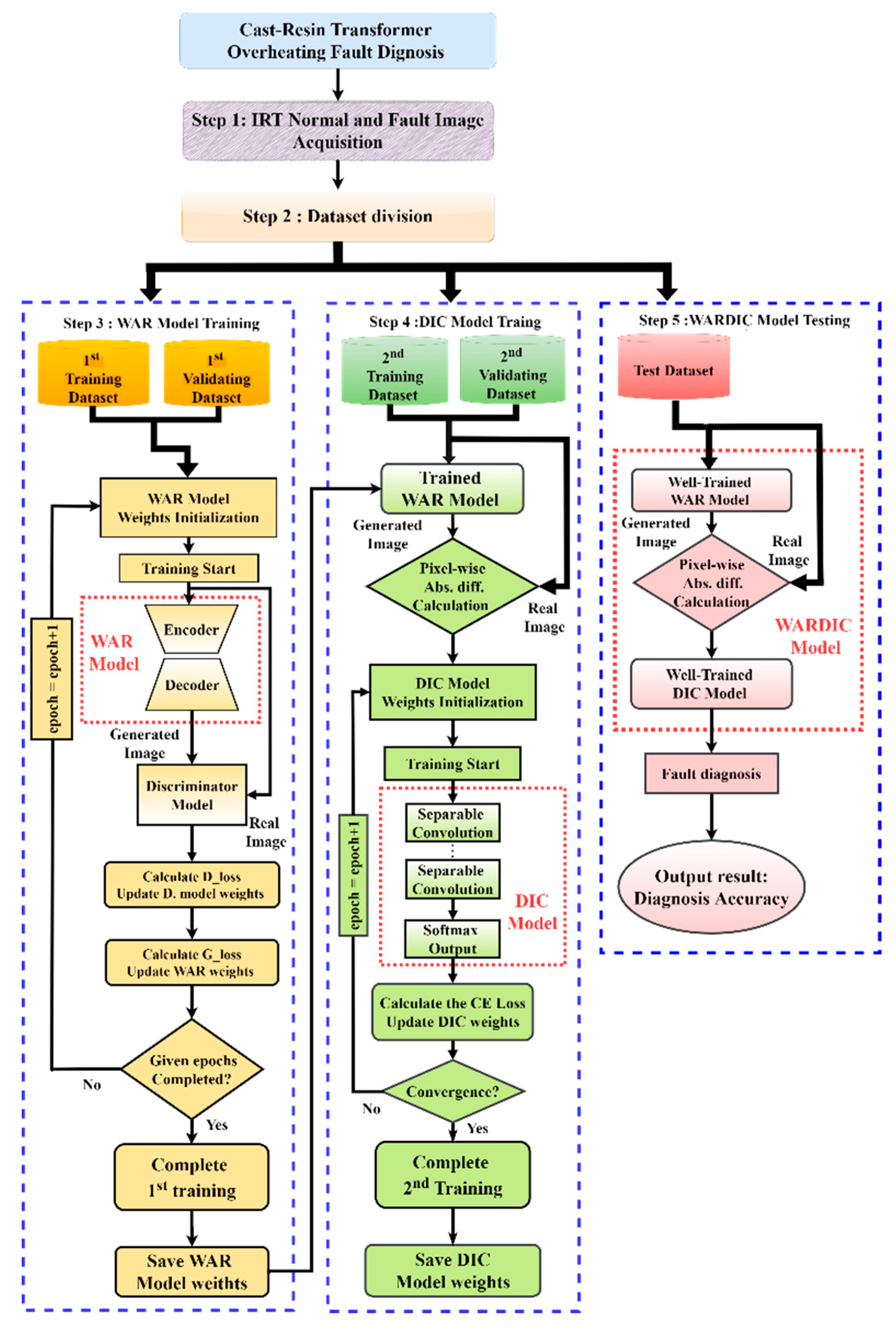
3. The Proposed Intelligent Fault Diagnosis Method

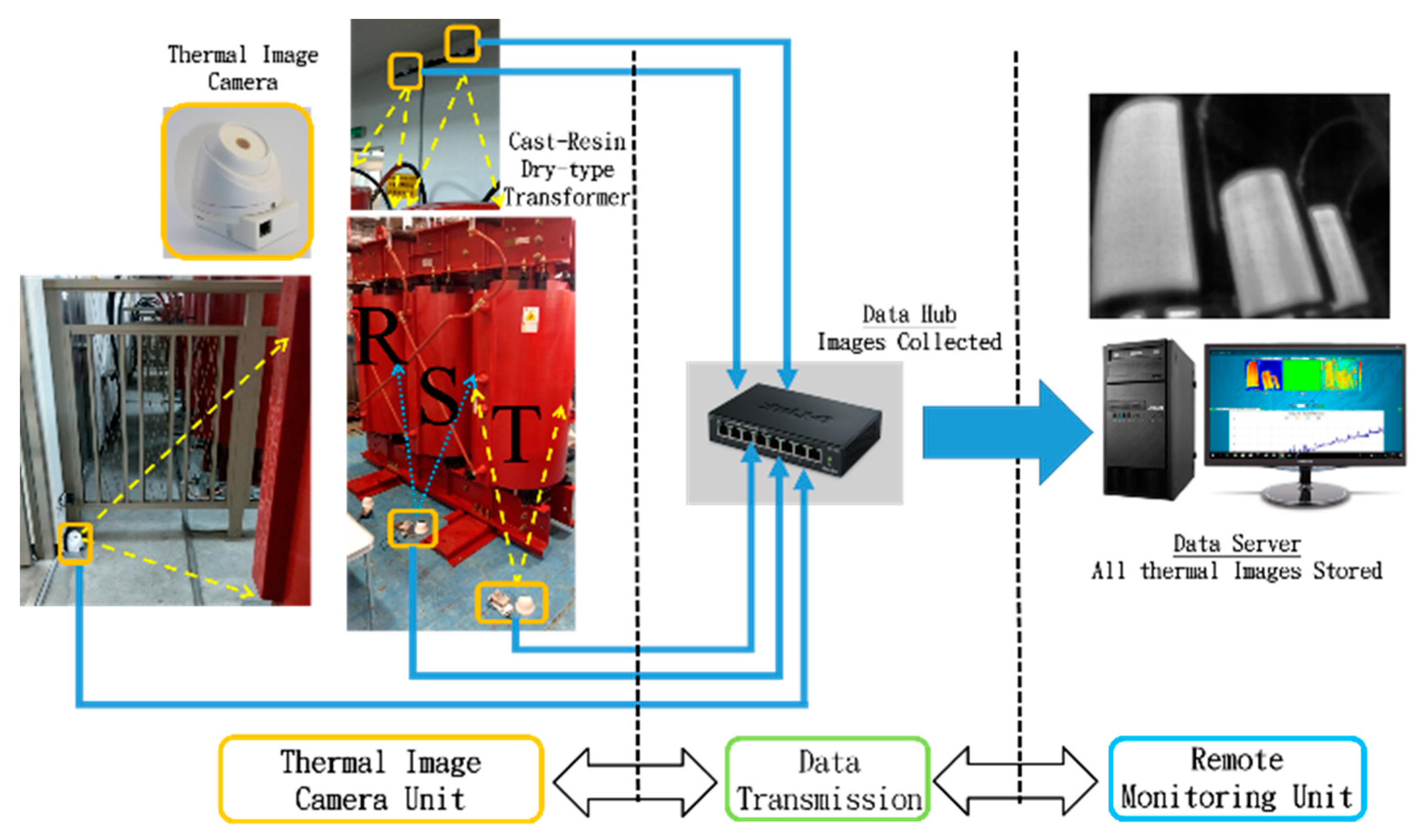
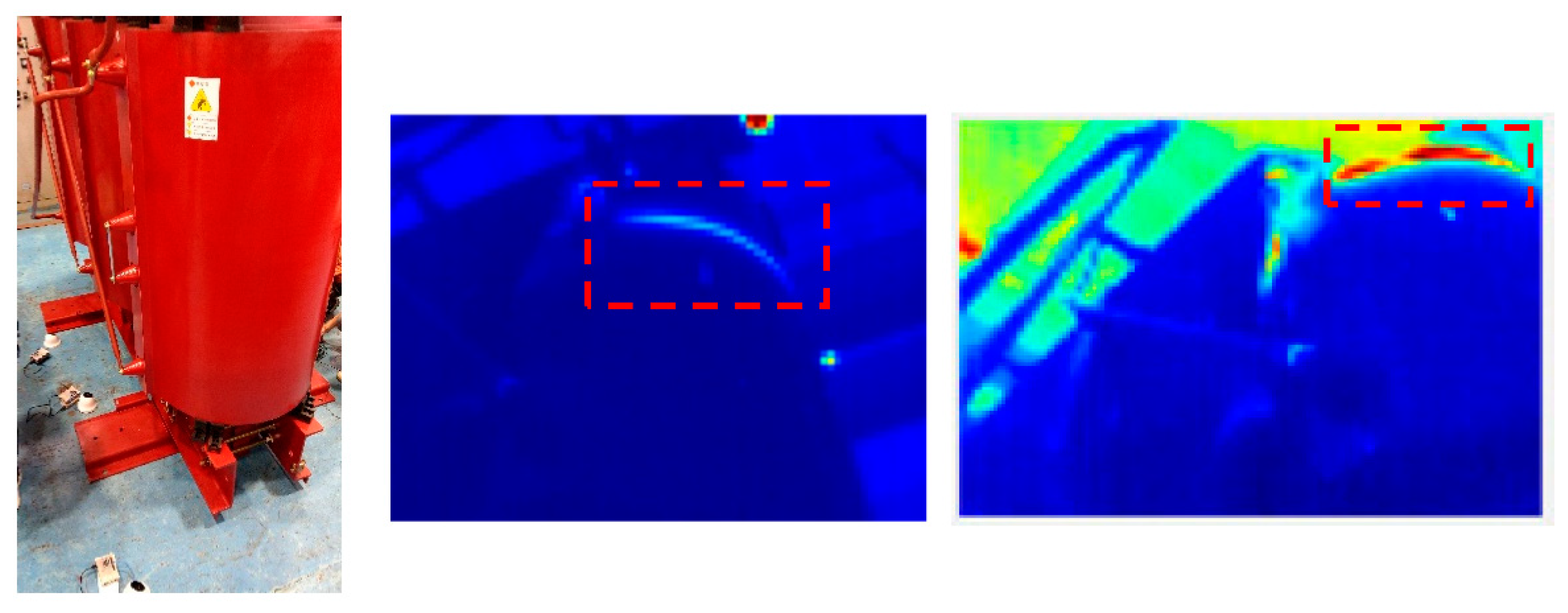
3.1. Overheating Fault Diagnosis System for Transformer-Based IRT Image

The experimental environment setting of cast-resin transformer is shown in Figure 1. Six sets of the thermal camera module are fixed on the ground or the ceiling about 0.8–1.2 m from the monitored three phase transformers. However, in this work, the IRT images were captured only by using a single thermal camera around the corner looking at the terminations and windings of the transformer at the thermographic windows. The infrared camera system is composed of a fixed-focus lens assembly, long-wave infrared (LWIR) microbolometer sensor array, and signal-processing electronics. The array format of thermal camera is 80 × 60 pixels available, which can measure object temperature up to 120 °C. Thermal images acquired by thermal camera are scaled to the resolution of 120 × 160 pixels via application of software. The field of view for diagonal and horizontal are 63.5° and 50° wide angle, respectively. The thermal sensitivity is of accuracy of about 0.05 °C. The thermal camera integrated with an ambient temperature sensor can measure the ambient temperature of the chip. The outputs of all cameras are assessable through Inter-Integrated Circuit communication protocol (I²C). The spirit of the proposed method is based on image comparison between the real running state and regenerated normal state. We only need to calculate the image difference between both states rather than the allowed difference of the temperature increase. As noted by the reviewer, in this work, the proposed method focusses on recognizing the fault type and the location of the fault. The voltage level of the transformer is 24 kV. The maximum ambient temperature, temperature-rise limitation and maximum permissible temperature are 40 °C, 100 K and 15 °C, respectively. The standard capacity, primary voltage and second voltage are 1000 KVA, 24 kV and 380 V, respectively. This system captures the normal condition images every 3 s and then they are stored on the remote server through the internet.

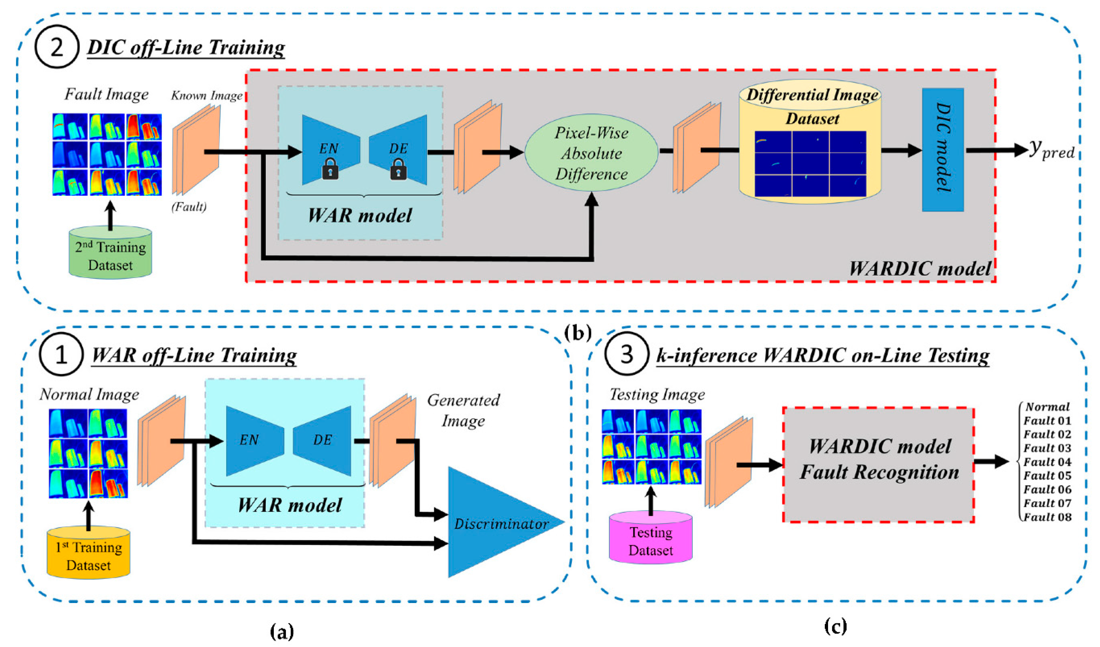
3.2. Design and Model Structure of the Proposed Networks

In this paper, an end-to-end network-structure-based IRT image for overheating fault diagnosis of cast-resin transformer, as seen in Figure 2, is proposed. Our method can be divided into three steps: (1) the WAR model off-line training, (2) the DIC model off-line training and (3) the k-inference WAR-DIC model on-line testing.

In order to design the lightweight networks for the use of fast fault monitoring and diagnosis on the edge device, the number of channels, filters, data lengths, stride size of the deep convolutional networks have an influence on the weight parameters and computational time. This paper proposes a method which contains two models: the WAR model and the DIC model. Firstly, the WAR model is designed to be trained with the normal IRT images. The main purpose of this model is to capture the characteristics of these normal images and to regenerate the pictures which are the same as the input images as much as possible. After the calculation of pixel-wise absolute difference between the input and regenerated images, the differential images are obtained and sent to the DIC model. Secondly, the DIC model is trained with the differential images which represent various kinds of fault trace. This model has the main task of quickly and correctly recognizing which kind of fault the input image is.

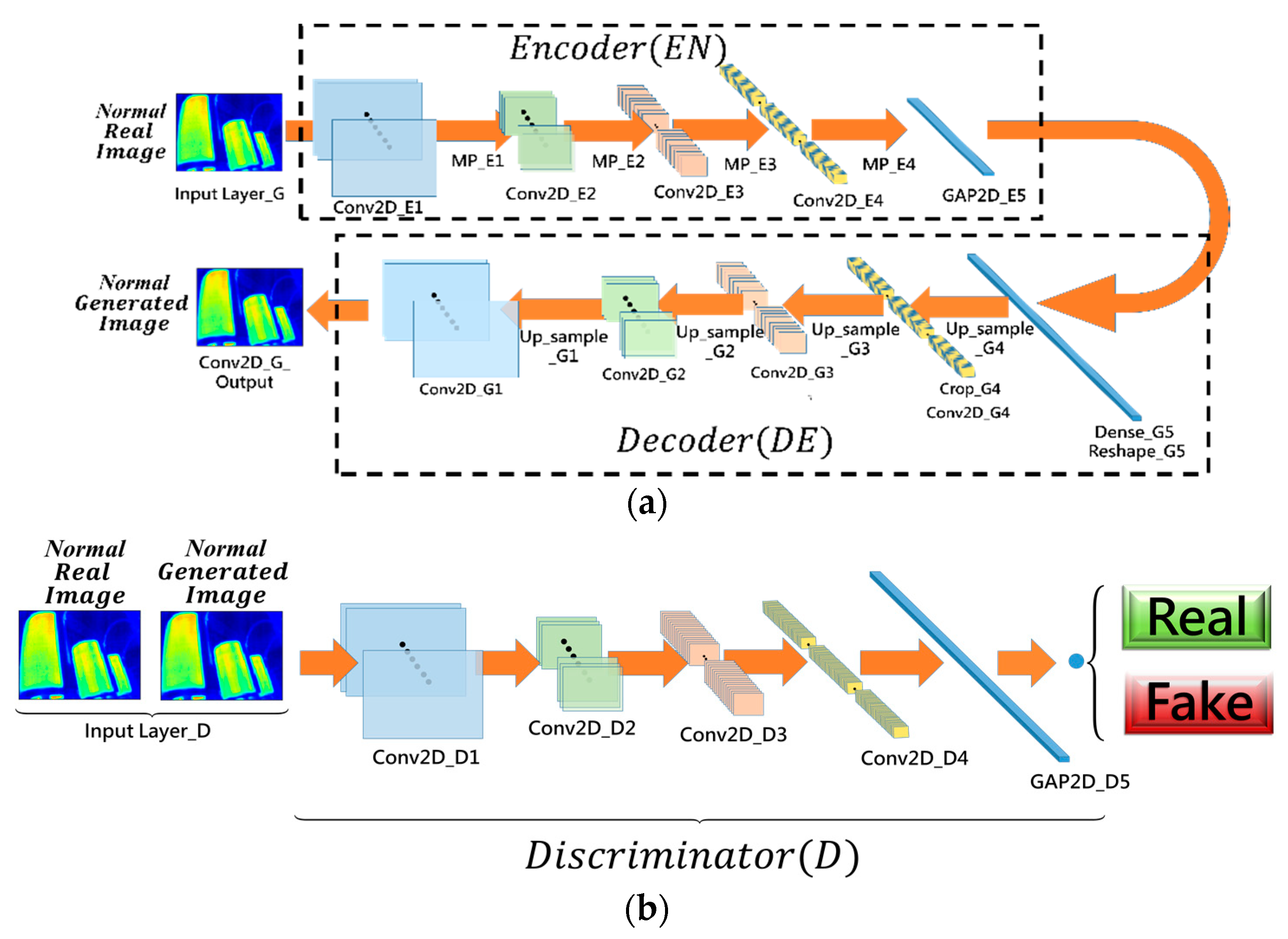
3.2.1. The WAR Model Off-Line Training

The process of the WAR model off-line training mainly has two networks: one is the WAR and the other is a discriminator network. The main purpose of the WAR is to regenerate the IRT image with normal state corresponding to the input data. The task of the discriminator is to manage to help the WAR reconstruct the normal image fast and precisely only at the training stage, not in use at the testing stage.

The WAR is based on a bow-tie autoencoder structure which is consisted of two parts: an encoder and a decoder. As shown in Figure 3a, the proposed encoder structure which has Conv2D_E1 to Conv2D_E4 convolution layers of the network included convolution operations, rectified linear unit (ReLU) activation functions. The function of batch normalization manages to keep the mean output be 0 and the output standard deviation be 1 for reducing the distribution of each layer’s input. After each convolution layer, the maximum pooling layer is used in the MP_E1 to MP_E4. At the end of the encoder, the global average pooling (GAP2D_E5) is used to reduce the number of weight parameters and avoid the overfitting.

The proposed decoder structure is also shown in Figure 3a. Following the output of the encoder, the dense layer (Dense_G5) is fully connected to the GAP2D_E5. The decoder has Conv2D_G4 to Conv2D_G1 convolution layers with ReLU and batch normalization. Before each convolution layer except the last one, the upsampling layer (UpSample2D_G1–UpSample2D_G4) is implemented to simply resize the image by means of interpolation because of not suffering from the checkerboard artifact. The output layer of the decoder is operated by a convolution layer with a sigmoid activation function which can convert the final output to a value between 0 and 1.

The proposed discriminator network is depicted in Figure 3b. This network contains four convolution layers (Conv2D_D1–Conv2D_D4) with ReLU and batch normalization. In addition to the first convolutional layer of the generator and discriminator network, features are extracted by using the convolution kernel with a side of 5 × 5, and then all the convolution kernels use the small convolution kernel of 3 × 3 for convolution operations. The final layer (Dense_D5) uses a linear activation function to approximate the Wasserstein distance divergence instead of sigmoid. The specific parameters settings of the WAR and discriminator networks are shown in

Table 2. The detailed structure of the WAR model.

Layer Type	Number of Kernel	Size of Kernel	Activation (DR Rate)	Output Shape
Input Layer_G	-	-	-	120 × 160 × 3
Conv2D_E1	8	5 × 5	ReLU/BN	120 × 160 × 8
MP_E1	-	2 × 2	-	60 × 80 × 8
Conv2D_E2	16	3 × 3	ReLU/BN	60 × 80 × 16
MP_E2		2 × 2		30 × 40 × 16
Conv2D_E3	24	3 × 3	ReLU/BN	30 × 40 × 24
MP_E3	-	2 × 2	-	15 × 20 × 24
Conv2D_E4	32	3 × 3	ReLU/BN	15 × 20 × 32
MP_E4	-	2 × 2	-	8 × 10 × 32
GAP2D_E5	-	-	-	32
Dense_G5	-	-	-	2560
Reshape_G5	-	-	-	8 × 10 × 32
Up_sample_G4	-	-	-	16 × 20 × 32
Crop_G4	-	-	(0, 1), (0, 0)	15 × 20 × 32
Conv2D_G4	32	3 × 3	ReLU/BN	15 × 20 × 32
Up_sample_G3	-	2 × 2	-	30 × 40 × 32
Conv2D_G3	24	3 × 3	ReLU/BN	30 × 40 × 24
Up_sample_G2	-	2 × 2	-	60 × 80 × 24
Conv2D_G2	16	3 × 3	ReLU/BN	60 × 80 × 16
Up_sample_G1	-	2 × 2	-	120 × 160 × 16
Conv2D_G1	8	3 × 3	ReLU/BN	120 × 160 × 8
Conv2D_G_Output	3	1 × 1	Sigmoid	120 × 160 × 3

and

Table 3. The detailed structure of the discriminator network.

Layer Type	Number of Kernel	Size of Kernel	Activation	Output Shape
Input Layer_D	-	-	-	120 × 160 × 3
Conv2D_D1	8	5 × 5	ReLU/BN	120 × 160 × 8
Conv2D_D2	16	3 × 3	ReLU/BN	60 × 80 × 16
Conv2D_D3	32	3 × 3	ReLU/BN	30 × 40 × 32
Conv2D_D4	128	3 × 3	ReLU/BN	15 × 20 × 128
GAP2D_D5	-	-	-	128
Dense_D5	-	-	Linear	1

.

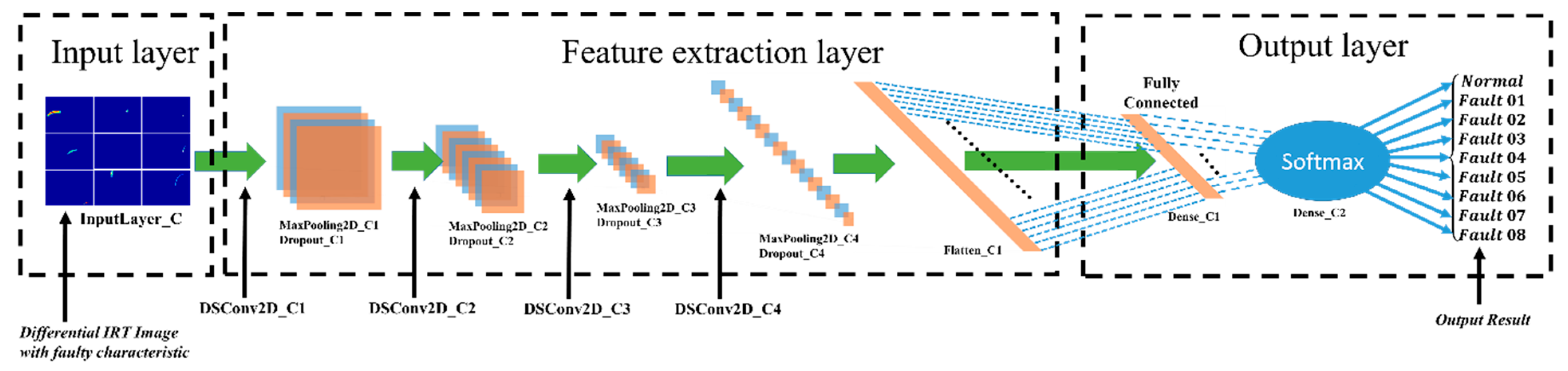
3.2.2. The DIC Model Off-Line Training

The proposed classification model aims to extract the finer information from the differential image after the calculation of pixel-wise absolute difference to recognize which kind of fault the input data is. As shown in Figure 4, the structure of this model structure has DSConv2D_C1 to DSConv2D_C4 depthwise separable convolution layers of the network include depthwise spatial and pointwise convolution, ReLU activation. Maximum pooling is used in the MP2D_C1 to MP2D_C4 to make the model have translation invariance and reduce the dimensionality of the input data. The dropout layer is also applied for the regularization constraint so that the model can capture more robust features by discarding a number of neurons. In this paper, there is only one fully connected layer (Dense_C1) with 16 nodes to get better performance through the experimental test. This results in reducing the large number of parameters of the classification. The output layer is usually connected to the Softmax layer for mapping to achieve the multiclassification task of IRT images. The specific parameter settings of the classification networks are shown in

Table 4. The detailed structure of the DIC model.

Layer Type	Number of Kernel	Size of Kernel	Activation	Output Shape
InputLayer_C	-	-	-	120 × 160 × 3
DSConv2D_C1	8	3 × 3	ReLU	120 × 160 × 8
MP2D_C1	-	2 × 2	-	60 × 80 × 8
DSConv2D_C2	16	3 × 3	ReLU	60 × 80 × 16
MP2D_C2	-	2 × 2	-	30 × 40 × 16
DSConv2D_C3	32	3 × 3	ReLU	30 × 40 × 32
MP2D_C3	-	2 × 2	-	15 × 20 × 32
DSConv2D_C4	64	3 × 3	ReLU	15 × 20 × 64
MP2D_C4	-	2 × 2	-	7 × 10 × 64
Flatten_C1	-	-	-	4480
Dense_C1	16	-	ReLU	16
OutputLayer_C	9	-	SoftMax	1

.

3.3. Diagnosis Procedure

The proposed method is utilized for diagnosing the overheating fault of the cast-resin transformer. The main procedure of the proposed method for fault diagnosis, as shown in Figure 5, can be outlined as follows:

Step 1: IRT normal and fault image acquisition. The IRT images with normal state and eight various fault condition of the cast-resin transformer are acquired by the thermal camera and saved on the remote monitoring system. After that, these images are gathered into the dataset and the training and testing of the WAR-DIC diagnosis model is conducted.

Step 2: All kinds of fault samples including normal state are randomly separated into the training dataset, the validation dataset and the testing dataset. The training process is divided into two parts: 1st training stage and 2nd training stage. At the 1st training stage, the training dataset is used for training the WAR model and the validation dataset is used for verifying the similarity between real and generated image of the trained WAR model. Both datasets of the 1st training stage only gather IRT images with normal state. At the 2nd training stage, the training dataset is used for training the DIC model. The validation dataset is used for verifying the accuracy of the trained DIC model. Both datasets of the 2nd training stage have eight categories of fault samples and one category of normal samples. The testing dataset is used for the inference of the fault classification and accuracy assessment of the trained WAR-DIC model. The validation dataset is composed by random selection from the testing dataset.

Step 3: At the 1st training stage, our WAR model with the discriminator is based on the concept of Wasserstein GAN [35] and GANomaly [36]. Firstly, the WAR model parameters are initialized. ${ℒ}_{d\_loss}$ and ${ℒ}_{g\_loss}$ are the discriminator loss and the WAR loss, respectively. Then the discriminator (D) is first updated several times via ${ℒ}_{d\_loss}$ to let the D distinguish the difference between the real image and the generated image. Next, the discriminator is fixed to train WAR via ${ℒ}_{g\_loss}$ once. Training D via minimizing ${ℒ}_{d\_loss}$in Equation (21) is exactly like the Wasserstein distance $W\left(p_r,p_g\right)$ divergence in Equation (6) [35].

$${ℒ}_{d\_loss}=-\left[D\left(x\right)\right]+\left[D\left(\widehat{x}\right)\right]$$

(21)

where $x$ and $\widehat{x}$ are the real images and the generated images, respectively.

The loss function of the WAR $({ℒ}_{g\_loss}$) proposed in this work has two loss values, the reconstruction loss ${ℒ}_{rec}$, the feature matching loss ${ℒ}_{fea}$ and the Wasserstein loss ${ℒ}_{was}$, in Equation (22).

$${ℒ}_{g\_loss}={\mathcal{W}}_{rec}{ℒ}_{rec}+{\mathcal{W}}_{fea}{ℒ}_{fea}+{\mathcal{W}}_{was}{ℒ}_{was}$$

(22)

where ${\mathcal{W}}_{rec}$, ${\mathcal{W}}_{fea}$,${\mathcal{W}}_{was}$ are the weighting constants adjusting the influence of each corresponding loss item to the total objective function.

The reconstruction loss ${ℒ}_{rec}$ is defined as Equation (23) and represents the error between the real and the generated images. The smaller the reconstruction loss, the closer the generated image is to the real image. In order to avoid yielding blurry results, this work also adopts the L1 distance to penalize the generator [44].

$${ℒ}_{rec}=\left|\right|x-{\widehat{x}\left|\right|}_1$$

(23)

The feature matching loss (${ℒ}_{fea}$) in Equation (24) is the error from the function $f()$between the feature representation of the real and the generated images. The function $f()$ is the intermediate output layer of the discriminator. ${ℒ}_{fea}$ calculates the L2 distance (Euclidean distance) to reduce the instability of GAN training,

$${ℒ}_{fea}=\left|\right|f\left(x\right)-f{\left(\widehat{x}\right)\left|\right|}_2$$

(24)

The Wasserstein loss (${ℒ}_{was}$) in Equation (25) is a way to train the generator model steadily to approach the distribution of the IRT image with normal state. The properties of the Wasserstein loss are continuous and differentiable. Therefore, the training process is more stable and less sensitive to model architecture. The larger scores for generated images the discriminator outputs, the smaller the WAR loss becomes.

$${ℒ}_{was}=-\left[D\left(\widehat{x}\right)\right]=-\left[D\left(G\left(x\right)\right)\right]$$

(25)

Further, to minimize the ${ℒ}_{d\_loss}$, let the $D\left(x\right)$ increase and the $D\left(\widehat{x}\right)$decrease. As for the ${ℒ}_{g\_loss}$, the smaller value ${ℒ}_{g\_loss}$ has, the smaller the difference between the real and the generated samples.

In order to assess the quality of the reconstructed image, the three common methods [37,38], PSNR in Equation (11), SSIM in Equation (12) and FID in Equation (16) are used for the criterion to compare between the real images and the generated images so as to find the better model. The higher the PSNR value is, the better the quality of the generated image is. SSIM gives the average value between 0 and 1 where the closer the value is to 1, the more similar both images are. A lower FID indicates that the distance between the generated data distribution and the actual data distribution is small. The FID score in the best case is 0, which means that the two sets of images are the same.

Step 4: At the 2nd training stage, the 2nd training dataset images are input first into the well-trained WAR model. Then, after the inference, the regenerated images are output and computed with the real images from the input by the calculation of pixel-wise absolute difference. Afterwards, this results in another dataset which is called the differential images dataset. Next, the DIC classification model parameters are initialized. The established DIC model is trained by the learning process of several epoch calculation until the given iterations are completed or the accuracy rate of the verification dataset achieves better performance. The CCE is used as the loss function in the classification model shown in Equation (26), and several fault types can be classified using the SR function shown in Equation (19). Further, the optimization algorithm adopted in the model has the advantages of the convergence characteristics in AdaGrad [45] and the momentum concept in Adam optimizer [46].

$$loss\left(\widehat{y},p\right)=-\frac{1}{n}{{\displaystyle \sum }}_{i=1}^n{{\displaystyle \sum }}_{j=1}^m{\widehat{y}}_{ij}log\left(p_{ij}\right)$$

(26)

Step 5: K-inference WAR-DIC online testing. The testing dataset data is fed into the trained WAR and DIC model. The recognition result of the overheating fault diagnosis for cast-resin transformer is output via the comparison and extraction of fault trace by using the trained model. The test process is an end-to-end process in which all we need to do is to directly input the original thermal image into this module and the module will produce the fault classification after inferential analysis.

4. Experiment Results and Comparisons

In this section, the proposed fault diagnosis model is conducted on the training, validating, and testing IRT image fault datasets of cast-resin transformer; this experiment is described in this section. Our method with the WAR-DIC model is compared with some existing methods, including traditional machine learning methods and other famous deep learning methods. The proposed method is implemented by Python 3.6 and Keras with Tensorflow as the backend. All the verifications and comparisons are run on Window 10 64 bit, using NVIDIA GTX 1650 GPU, except the inference time testing without GPU running on Google Colaboratory.

4.1. Dataset Description

For sensing the phenomenon of temperature-rising caused by overcurrent, most cast-resin transformers have added a PTC (positive temperature coefficient) thermal fuse, which is combined with the low-voltage coil. However, at the high voltage coils, local overheating can often occur because of interturn short circuits arising from the demolition of the solid insulation by partial discharge. Local overheating is regarded as the previous warning of the failure probably leading to burning. If detected early, the disconnection of the transformer can be done in a timely manner to avoid consequential damages. Figure 6 shows the real infrared thermography detecting the interturn short-circuit in the cast-resin transformer. Using a thermal camera to observe the transformer with the short-circuit interturn, it can be seen that heat energy is transmitted by the short-circuited coil. Figure 6 also shows obvious overheating aperture surrounding the periphery of the transformer coil, which indicates the region where the fault has occurred. Based on the above observation, we use the thermal image monitoring system proposed in this paper to capture normal and fault IRT images under different load conditions and different faulty positions.

In order to verify the effectiveness of the proposed method, there is one normal condition and eight fault conditions, corresponding to label Fault 00 and Fault 01 to Fault 08, respectively. The normal state marked “F0” has captured 3000 samples. The interturn short circuit of the R, S, and T phases are marked as F1, F2 and F3, respectively. The interturn short-circuit often occurs in the winding insulation deterioration fault of dry-type transformers. In the early stage of the fault, due to the deterioration of the high-voltage winding insulation layer, the interlayer discharge damage is caused, which causes the winding to be short-circuited, the current rises and the temperature rises.

The connection overheating of phase R, S and T are marked as F4, F5 and F6, respectively. The connection overheating fault usually occurs at the connection between the primary side and the secondary side, and the contact surface is usually locked with screws to transmit the current. Factors such as loose connection, overload, unbalanced load due to construction or excitation vibration may cause overheating. The main heat source is the contact point. As the passing current increases, the temperature also rises. Obvious hot spots can be observed through the thermal image. The overheating of the wires in the S and T phases is marked as F7 and F8. Overheating of the wires occurs in the connecting cable with the transformer, which usually causes heat due to overload, unbalanced load, load failure and other reasons.

Each of the eight fault conditions is captured for 2000 samples for the training and testing. Each sample is an IRT image with 120 × 160 × 3 pixels. In the first stage of the training process, there are 1000 images only with normal state for use as the training dataset.

In the second stage of the training process, four different imbalanced degree datasets (Dataset 2A, 2B, 2C and 2D) are gathered. Dataset 2A is a balanced dataset. There are 2000 no-fault images and 2000 images for each fault, which is divided in two equal part for training and testing. The total number of training samples is 9000, which is the same as that of the test samples. Datasets 2B, 2C and 2D are used to simulate the imbalanced classification. In a real case, it is much more difficult to capture the abnormal samples than the normal ones. In this paper, the 50%, 20% and 10% of each fault sample of Dataset 2A except for normal samples (F0) is respectively composed of the Dataset 2B, 2C, 2D. For ease of comparison studies, the testing samples are still 1000 for each fault, including the normal case. Dataset 2D is considered the more imbalanced dataset than other datasets due to the smaller number e of training fault samples. The detailed description of the experimental data is shown in

Table 5. The detailed description of the faulty IRT image dataset.

Cast-Resin Transformer Fault Type		Label	Number of Training Dataset					Number of Testing Datasets
			1st Training for WAR	2nd Training for DIC
			Dataset 1	Dataset 2A	Dataset 2B	Dataset 2C	Dataset 2D
Normal		F0	1000	1000	1000	1000	1000	1000
Interturn short circuit	(R)	F1	-	1000	500	200	100	1000
	(S)	F2	-	1000	500	200	100	1000
	(T)	F3	-	1000	500	200	100	1000
Connection overheating	(R)	F4	-	1000	500	200	100	1000
	(S)	F5	-	1000	500	200	100	1000
	(T)	F6	-	1000	500	200	100	1000
Wire overheating	(S)	F7	-	1000	500	200	100	1000
	(T)	F8	-	1000	500	200	100	1000

. Therefore, there are a total of nine types of transformer conditions, as shown in Figure 7. The differential IRT image is obtained by calculating the difference between the original real image and the generated image from the WAR model. The differential image highlights the location of the fault. For this reason, the proposed method can diagnose the IRT image without the need to search for ROI preprocessing in advance.

4.2. Results and Discussion

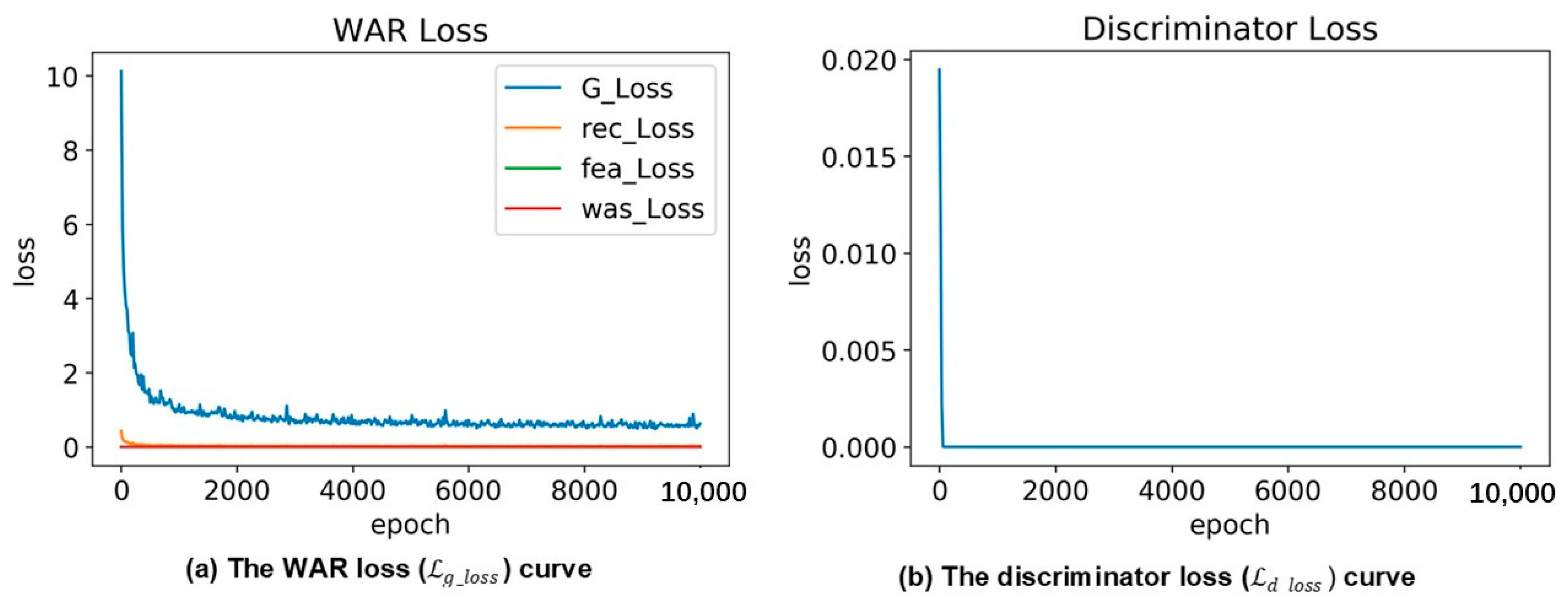
4.2.1. Evaluation Result of the WAR Model

In the first stage of training, the reconstruction model is trained to learn and extract features from 1000 normal state samples. When training the WAR model, Adam optimizer with a learning rate of 0.001 is conducted. The batch size is 64. The 1st training epoch is set to 10,000. In order to select the best WAR model, this paper utilizes the FID evaluation to monitor the training process. The WAR loss function in Equation (22) has weights of ${\mathcal{W}}_{rec}$ = 20, ${\mathcal{W}}_{fea}$ = 1 and ${\mathcal{W}}_{was}$ = 5. As shown in Figure 8, after 10,000 epochs of training, the WAR loss and discriminator loss are recorded every 20 epochs. As can be seen from Figure 8, after only 1800 epochs, loss values of the WAR (${ℒ}_{g\_loss}$) and the discriminator (${ℒ}_{g\_loss}$) have become stable. The model has begun gradually to converge. This paper takes the top 10 FID scores after 10,000 epochs of training process, as shown in

Table 6. The training values of FID, Mean_SSIM and Mean_PSNR of the WAR model.

Epoch	FID	Mean_SSIM	Mean_PSNR
4700	0.447291	0.999919	76.433
5540	0.288334	0.999837	75.162
6420	0.316712	0.999927	77.061
7000	0.295348	0.999757	73.630
7040	0.299828	0.999765	74.588
8240	0.298133	0.999734	74.416
8320	0.276073	0.999832	75.667
8400	0.299400	0.999772	74.258
9500	0.256580	0.999874	76.293
9540	0.257940	0.999856	75.998

. Meanwhile, the evaluation of SSIM and PSNR for the WAR model are also considered. The Mean_SSIM and Mean_PSNR in Table 6, respectively, represent the average value of SSIM and PSNR after calculating each of the 200 normal images in the validation dataset. Following the above evaluation, we think that the WAR model at epoch = 6420 in Table 6 is the best selection because of better Mean_SSIM and Mean_PSNR than others, albeit without the lowest FID score. As the result of the 1st training, we take this model to generate normal images in the 2nd training process.

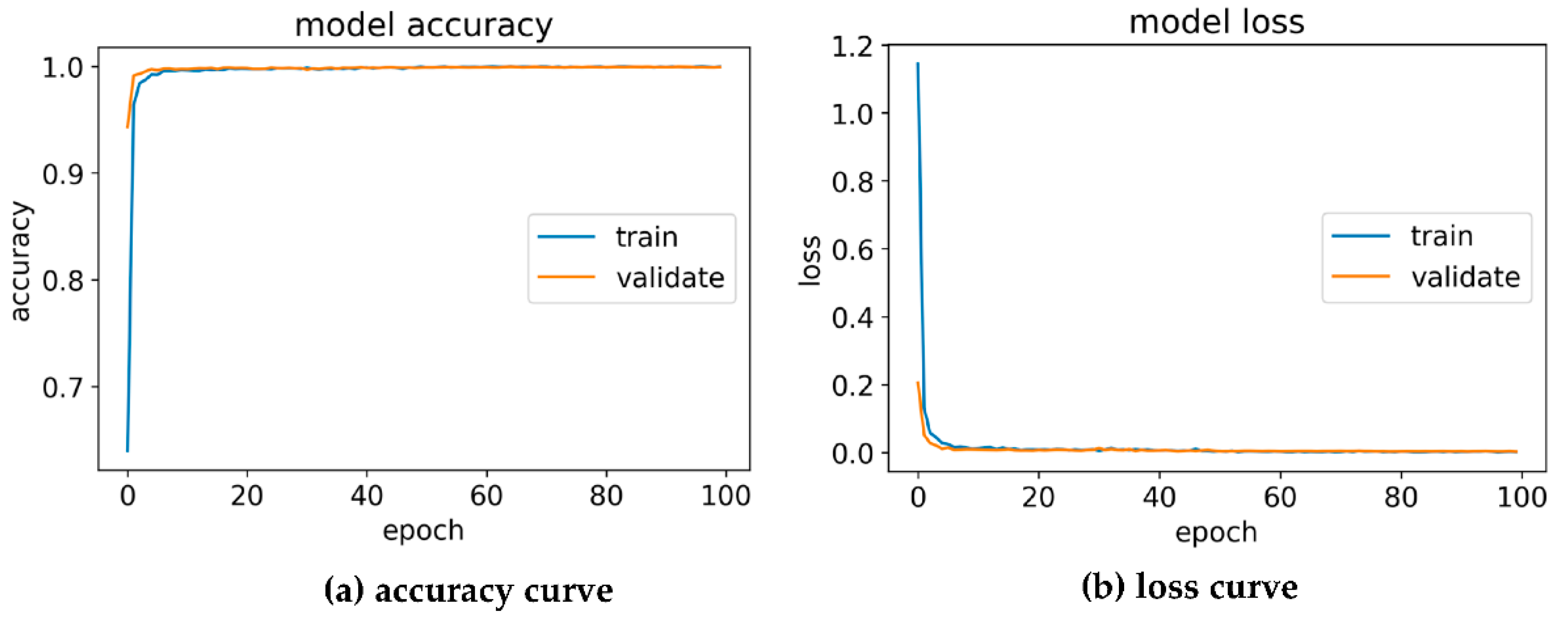
4.2.2. Evaluation Result of the DIC Model

In the second stage of training, the IRT real images of datasets 2A, 2B, 2C, 2D are firstly input to the trained reconstruction model to obtain the generated images. After calculation of pixel-wise absolute difference, the corresponding differential images dataset is achieved for use in training the DIC model. The accuracy curve and loss curve of the DIC model in the 2nd training are shown in Figure 9. The training parameters of the DIC model are set to a learning rate of 0.001, an epoch of 100 and a batch size of 64. For the training process, we randomly select 200 images of each fault type except normal state (F0) from the testing dataset as the validation dataset for the sake of getting the best model. As can be seen from Figure 9, when training after 30 epochs, the accuracy and loss have begun to stabilize with less change, which means that the DIC model has a robust convergence ability.

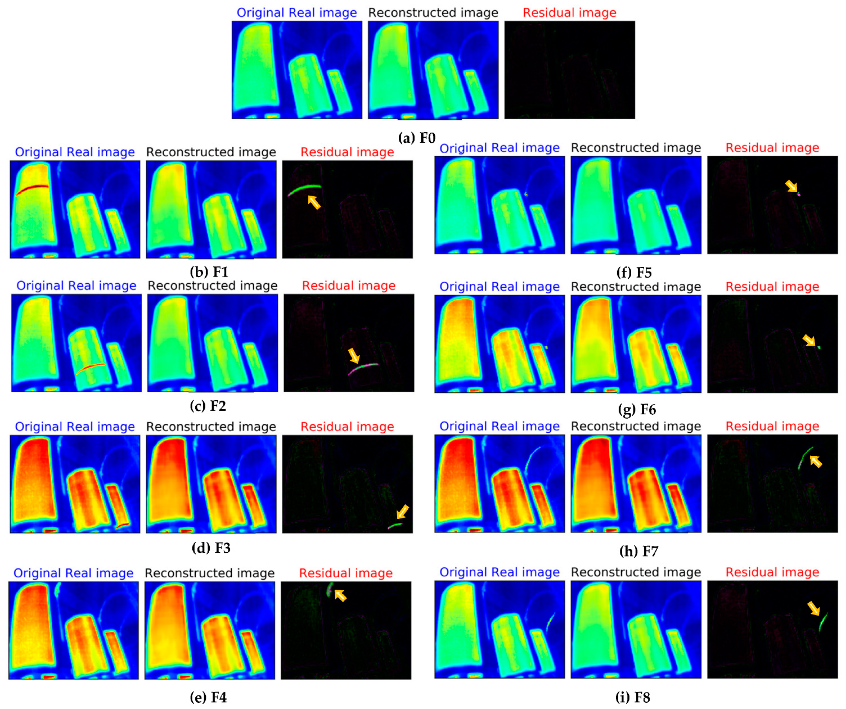
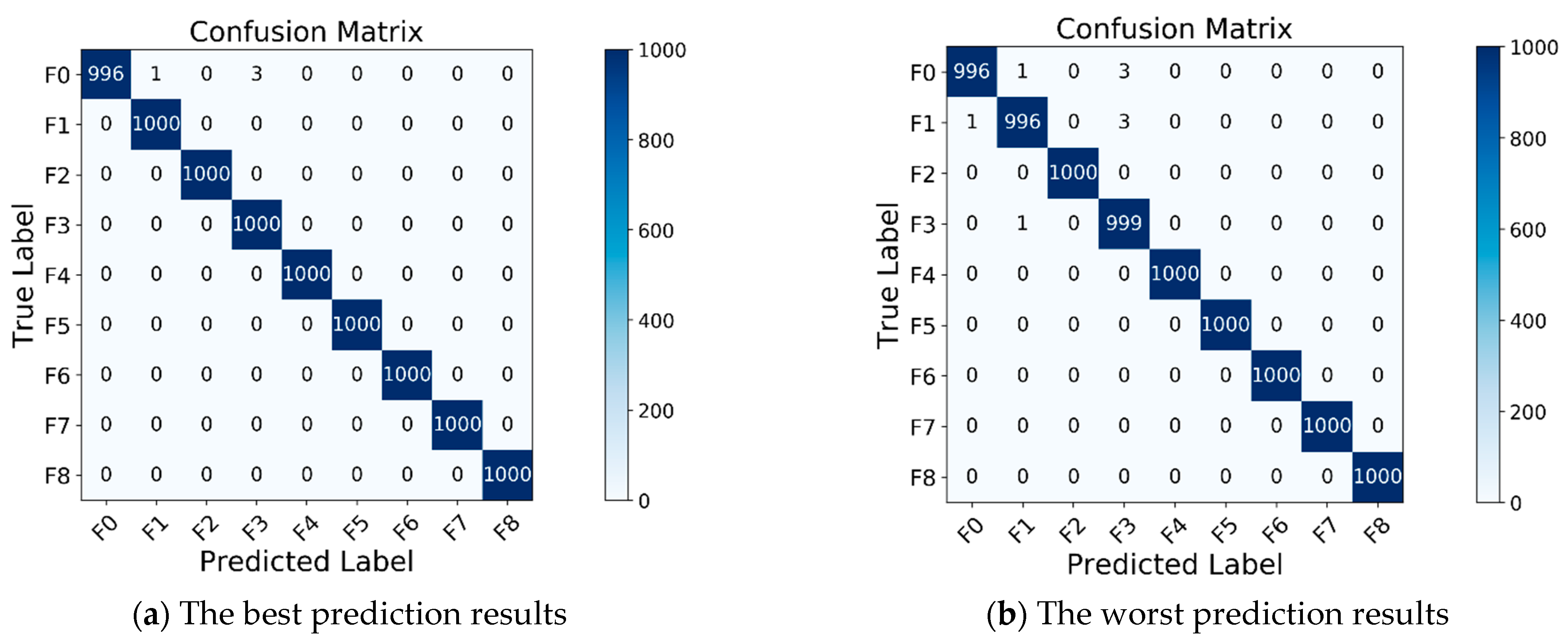
4.2.3. Testing Result of the WAR-DIC Model

The trained WAR-DIC model is used to categorize the testing dataset for the acquisition of the classification accuracy. In this paper, the proposed WAR-DIC model was run for training 10 trials under each different training dataset to confirm the reliability and stability of the model and reduce the influence of randomness. The accuracy results of maximum (Max.), minimum (Min.), mean and standard deviation (Std) based on the same testing dataset are listed in

Table 7. The testing result of the proposed WAR-DIC model in different imbalance training datasets.

Training Dataset	Max. Accuracy	Max. Accuracy	Mean Accuracy	Std
2A	99.95%	99.91%	99.92%	0.0235%
2B	99.88%	99.78%	99.86%	0.0228%
2C	99.71%	99.65%	99.69%	0.0205%
2D	99.45%	99.38%	99.42%	0.0219%

. According to the results in Table 7, the DIC model trained on dataset 2A performed with 99.92% ± 0.0235% accuracy on the testing set. In addition, to validate the ability of imbalanced fault classification, three different imbalance degree training datasets are conducted in the experiment. Table 7 also shows the testing accuracy result for different models trained on datasets 2B, 2C, 2D. The WAR-DIC model also achieved better average testing accuracy of 99.86% ± 0.0288%, 99.69% ± 0.0205% and 99.42% ± 0.0219%, respectively, under different imbalance training with 2B, 2C and 2D datasets.

To detail the classification results for the model trained on dataset 2A, the confusion matrix representations of the best and worst testing results (the maximum and minimum testing accuracy for training dataset 2A in Table 7) are shown in Figure 10. In Figure 10, the rows indicate the ground truth label for each fault sample and the columns represent the predicted label of each fault sample. From the confusion matrix of the best prediction testing result, the predicted testing accuracy for all fault samples is 100%, except F0, four F0 samples are misclassified as one F1 sample and three F3 samples. Specifically, no fault samples were misjudged as normal samples except for the F1 of the worst prediction result. The results of the precision, sensitivity and specificity analysis on the confusion matrix of the best prediction result are outlined in

Table 8. The testing results of the confusion matrix of the best prediction WAR-DIC model trained on dataset 2A.

Fault Type	Precision	Sensitivity	Specificity	Accuracy
F0	100%	99.60%	100%	99.95%
F1	100%	99.90%	99.98%
F2	100%	100%	100%
F3	99.50%	100%	99.96%
F4	100%	100%	100%
F5	100%	100%	100%
F6	100%	100%	100%
F7	100%	100%	100%
F8	100%	100%	100%

. The analysis result shows that except for the precision of F3 of 99.50% and the sensitivity of F0 of 99.60%, the precision, sensitivity, specificity of all other conditions can achieve more than 99.90%, which demonstrates the effectiveness of this proposed method.

4.3. Performance Analysis of the Network Parameters

Several lightweight and classic network structures have been proposed in recent years, such as ShuffleNet, MobileNetV1, SqueezeNet, LeNet5, ResNet-50, VGG-16, which are compared in terms of the number of the total parameters, weight storage and the floating-point computations, as shown in

Table 9. Comparison of networks in terms of parameter, weight storage and computational load.

Method	Number of Total Parameters (Million)	Floating-Point Computations (Million)	Weight Storage (MB)
ShuffleNet	3.903	64.875	31.725
MobileNetV1	3.494	58.697	27.513
SqueezeNet	0.378	2.27	3.068
LeNet5	6.448	77.379	50.406
ResNet-50	24.115	408.620	188.794
VGG-16	14.849	252.392	116.103
Ours	0.223	1.781	1.837

.

ShuffleNet is a lightweight neural network based on the concept of 1 × 1 group convolution proposed in [28] in order to reduce the amount of calculation and ensure classification accuracy. MobileNetV1 [27], proposed by Google, uses depthwise separable convolution without a pooling layer to further reduce the model size and calculation amount. For the flexible deployment to memory-limited hardware, SqueezeNet [26] can achieve the approximate accuracy of AlexNet [47] on the ImageNet dataset, but the parameters are 50 times fewer than those of AlexNet, LeNet5 [48], ResNet-50 [49], VGG-16 [50], which are commonly used for machinery fault diagnosis.

The proposed method in this paper consists of three parts: the WAR model, the calculation of pixel-wise absolute difference and the DIC model. The calculation of pixel-wise absolute difference has no parameters so that the floating-point computation can be ignored. The number of parameters, weight storage and floating-point computation of the proposed method are each performed on the sum of that of both models. To accommodate the IRT image size in this paper, the input shape of these six networks and the proposed method are modified to 120 × 160 × 3 for the calculation process.

The results shown in Table 9 indicate that the proposed method is 2 orders of magnitude smaller than ResNet-50, VGG-16 and at least 40 times smaller than LeNet5 in terms of floating-point computation, and the number of parameters of the proposed method is almost one-hundredth of that of ResNet-50, VGG-16, and approximately one-thirtieth of that of LeNet5. As for other lightweight network, the computation loads of ShuffleNet, MobileNetV1 are 36.43, 32.96 times that of the proposed method. The number of parameters of the proposed method is only 5.7% of that of ShuffleNet, 6.3% of that of MobileNetV1. SqueezeNet has good performance on the smallest amount of parameters and the least storage space compared to other trained lightweight and classic models. However, the proposed method still has advantages in the number of weights, computational loads and storage space. The number of parameters, floating-point computation and storage space of the proposed method is respectively 58.99%, 78.45% and 59.88% of that of SqueezeNet. The proposed method has a stronger ability to extract features, which can be seen in subsequent experiments.

4.4. Comparison with Other Methods

To evaluate the performance of the proposed model presented in this paper, Support Vector Machine (SVM), Random Forest (RF), Decision Tree (DT), traditional classic CNN such as LeNet5, VGG-16, ResNet50 and common lightweight CNN such as ShuffleNet, MobileNet, SqueezeNet are selected for comparison with the proposed method. For fairness and consistency of comparison, the experiments were performed using the same various imbalanced training dataset and testing datasets. The diagnosis results are presented in

Table 10. The comparison results of different methods and the proposed method.

Method	Classification Accuracy				Inference Time (sec/1.8 K Images)
	2A	2B	2C	2D
SVM	98.56%	97.84%	94.50%	87.34%	287.59
RF	98.51%	94.64%	95.52%	86.28%	0.21
DT	97.39%	91.87%	84.62%	76.86%	0.09
ShuffleNet	99.93%	99.78%	99.31%	11.13%	90.44
MobileNetV1	99.92%	99.75%	98.65%	11.11%	78.10
SqueezeNet	99.90%	99.83%	99.44%	99.15%	24.62
LeNet5	99.94%	99.63%	99.57%	98.82%	26.83
ResNet-50	99.96%	99.90%	99.32%	98.94%	86.94
VGG-16	99.96%	99.95%	11.11%	11.11%	346.33
Ours	99.95%	99.89%	99.71%	99.46%	28.53

.

As can be seen in Table 10, the diagnostic accuracy of the proposed method on training datasets 2A, 2B, 2C, 2D is respectively 99.95%, 99.89%, 99.71%, 99.46%, significantly higher than that of the other models, except for training datasets 2A and 2B. The experimental results show that the proposed algorithm exhibits the second highest performance on datasets 2A and 2B. Although ResNet-50 and VGG-16 outperform the proposed method with 0.01% on dataset 2A and with 0.07% on dataset 2B, the number of parameters of ResNet-50 and VGG-16 is more than 108.14 and 66.58 times more than that of the proposed method, as shown in Table 9. Specifically, the fault diagnosis accuracy of SVM on training datasets 2A, 2B, 2C, 2D is 98.55%, 97.84%, 94.50% and 87.82%, RF’s accuracy is 98.51%, 94.64%, 95.52%, 86.28%, DT’s accuracy is 97.38%, 91.87%, 84.62%, 76.44%, ShuffleNet’s accuracy is 99.93%, 99.78%, 99.31% and 11.13%, MobileNetV1′s accuracy is 99.22%, 99.75%, 98.65%, 11.11%, SqueezeNet’s accuracy is 99.90%, 99.83%, 99.43%, 99.15%, LeNet5′s accuracy is 99.94%, 99.63%, 99.57%, 98.82%, ResNet-50′s accuracy is 99.96%, 99.90%, 99.32%, 98.94%, and VGG-16′s accuracy is 99.96%, 99.95%, 11.11%, 11.11%.

Datasets 2B, 2C and 2D are considered to simulate various models for imbalanced classification problems. Although prediction accuracy is regarded as the most useful evaluation for classification, it is improper for imbalanced classification tasks. In the multiclass imbalanced classification problem, the alternative way to solve these issues is to select precision, recall metrics and ROC AUC score as the assessment metric for an imbalanced learning model [51]. Precision represents the quantification of positive class predictions that actually belong to the positive class. Recall represents the quantification of how well the positive class was predicted. Precision and Recall are defined as follows:

$$\mathrm{Precision}=\frac{\mathrm{TP}}{\mathrm{TP}+\mathrm{FP}}$$

(27)

$$\mathrm{Recall}=\frac{\mathrm{TP}}{\mathrm{TP}+\mathrm{FN}}$$

(28)

where TP (true positive) means that correct samples are correctly recognized. FP (false positive) means that incorrect samples are regarded as correct. FN (false negative) means that correct samples are regarded as incorrect. TN (true negative) means that incorrect samples are correctly recognized.

Receiver operating characteristic (ROC) represent the definition of the comparison between true positive rate (TPR) and false positive rate (FPR) under various thresholds. The TPR and FPR are defined as follows:

$$\mathrm{TPR}=\frac{\mathrm{TP}}{\mathrm{TP}+\mathrm{FN}}$$

(29)

$$\mathrm{FPR}=\frac{\mathrm{FP}}{\mathrm{FP}+\mathrm{TN}}$$

(30)

ROC can be drawn as a curve that plots all pairs of the TPR and the FPR to compare the performance with other models. Area under the curve (AUC) is the fraction of the area covered under the ROC curve divided by the ratio of the total area. The value range of AUC is generally between 0 and 1. The higher the AUC score, the better the classifier performance. From the results shown in

Table 11. The comparison results for imbalanced training dataset 2D.

Method	Precision	Recall	Specificity	ROC AUC
SVM	88.63%	87.34%	98.41%	0.982382
RF	90.99%	85.82%	98.23%	0.991549
DT	78.05%	76.87%	97.11%	0.869988
SqueezeNet	99.22%	99.16%	99.89%	0.999951
LeNet5	98.28%	99.78%	98.51%	0.999961
ResNet 50	99.03%	98.94%	99.87%	0.999930
Ours	99.46%	99.45%	99.93%	0.999971

, the proposed method outperforms other methods in a multiclass imbalanced classification. In real-world application, it is much easier to collect the normal state images rather than the fault images. Under the imbalanced training dataset, our method has good performance for classification accuracy.

As for the CPU inference times, the inference time of the proposed method is the sum of the reconstruction time, calculation time of pixel-wise absolute difference and classification testing time. Besides RF and DT, SqueezeNet takes the shortest time, followed by LeNet5, the proposed method, MobileNetV1, ResNet-50, ShuffleNet, SVM and VGG-16. Although the inference time of RF and DT is less than 1 s, we do not consider both methods for comparison due to worse accuracy. After analyzing various indicators, such as fault classification accuracy, model parameters, storage size, inference time and imbalanced training dataset, it can be seen that the proposed model presented in this paper has better performance.

5. Conclusions

This paper presents a full-time online fault monitoring system for cast-resin transformer and proposes an overheating fault diagnosis method based on the WAR-DIC model. The proposed system can detect nine different types of cast-resin transformer from IRT images taken by the fastened thermal camera.

The WAR-DIC network structure can effectively reduce the amount of the model parameters and storage size, and ensure the classification accuracy and fast calculation speed when compared with other common methods. The mean accuracy after 10 runs of the proposed WAR-DIC model for balanced training dataset and worst imbalanced training dataset are respectively 99.92% ± 0.0235% and 99.42% ± 0.0219%. The number of parameters, weight storage and floating-point computation of the proposed method are 0.223 million, 1.781 million and 1.837 MB.

This paper also compared the evaluation testing results of different classic CNN (LeNet5, ResNet50, VGG16), lightweight CNN (SqueezeNet, MobileNetV1, ShuffleNet) and conventional machine learning method (SVM, RF, DT) under different imbalanced training dataset. All these testing results show that the proposed model with smaller size and fewer parameters can even still maintain good classification accuracy. Comparisons with previous studies verified the superior performance of the proposed system.

Some future research will be conducted in the following aspects. Firstly, this WAR-DIC model will be applied for different scenarios with an overheat situation, such as fault detection of power inverter. Secondly, given that it is difficult to collect all the fault patterns in the training phase, we will try to push the existing WAR-DIC model to learn for open-set fault diagnosis in an unsupervised or semi-supervised learning. Thirdly, the proposed method is limited by the inability to detect the initial stage of failure without overheating. We consider that future research will focus on combining two-or-more-sensor data to overcome the abovementioned issue.

References

1. Chen, P.; Huang, Y.; Zeng, F.; Jin, Y.; Zhao, X.; Wang, J. Review on insulation and reliability of dry-type transformer. In Proceedings of the 2019 IEEE Sustainable Power and Energy Conference (iSPEC), Beijing, China, 20–24 November 2019. [Google Scholar]
2. Mafra, R.; Magalhães, E.; Anselmo, B.; Belchior, F.; Lima e Silva, S.M.M. Winding hottest-spot temperature analysis in dry-type transformer using numerical simulation. Energies 2018, 12, 68. [Google Scholar] [CrossRef] [Green Version]
3. Duan, X.; Zhao, T.; Liu, J.; Zhang, L.; Zou, L. Analysis of Winding Vibration Characteristics of Power Transformers Based on the Finite-Element Method. Energies 2018, 11, 2404. [Google Scholar] [CrossRef] [Green Version]
4. Senobari, R.K.; Sadeh, J.; Borsi, H. Frequency response analysis (FRA) of transformers as a tool for fault detection and location: A review. Electric. Power Syst. Res. 2018, 155, 172–183. [Google Scholar] [CrossRef]
5. Zhang, Z.; Gao, W.; Kari, T.; Lin, H. Identification of Power Transformer Winding Fault Types by a Hierarchical Dimension Reduction Classifier. Energies 2018, 11, 2434. [Google Scholar] [CrossRef] [Green Version]
6. Li, E.; Wang, L.; Song, B.; Jian, S. Improved Fuzzy C-Means Clustering for Transformer Fault Diagnosis Using Dissolved Gas Analysis Data. Energies 2018, 11, 2344. [Google Scholar] [CrossRef] [Green Version]
7. Bagheri, M.; Zollanvari, A.; Nezhivenko, S. Transformer fault condition prognosis using vibration signals over cloud environment. IEEE Access 2018, 6, 9862–9874. [Google Scholar] [CrossRef]
8. Sun, Y.; Hua, Y.; Wang, E.; Li, N.; Ma, S.; Zhang, L.; Hu, Y. A temperature-based fault pre-warning method for the dry-type transformer in the offshore oil platform. Int. J. Electr. Power Energy Syst. 2020, 123, 106218. [Google Scholar] [CrossRef]
9. Chen, M.-K.; Chen, J.-M.; Cheng, C.-Y. Partial discharge detection in 11.4 kV cast resin power transformer. IEEE Trans. Dielectr. Electr. Insul. 2016, 23, 2223–2231. [Google Scholar] [CrossRef]
10. Athikessavan, S.C.; Jeyasankar, E.; Manohar, S.S.; Panda, S.K. Inter-turn fault detection of dry-type transformers using core-leakage fluxes. IEEE Trans. Power Deliv. 2019, 34, 1230–1241. [Google Scholar] [CrossRef]
11. Gockenbach, E.; Werle, P.; Borsi, H. Monitoring and diagnostic systems for dry type transformers. In Proceedings of the ICSD’01 2001 IEEE 7th International Conference on Solid Dielectrics (Cat. No.01CH37117), Eindhoven, The Netherlands, 25–29 June 2001. [Google Scholar] [CrossRef]
12. Lee, C.-T.; Horng, S.-C. Abnormality detection of cast-resin transformers using the fuzzy logic clustering decision tree. Energies 2020, 13, 2546. [Google Scholar] [CrossRef]
13. Tang, S.; Hale, C.; Thaker, H. Reliability modeling of power transformers with maintenance outage. Syst. Sci. Control Eng. 2014, 2, 316–324. [Google Scholar] [CrossRef]
14. Tenbohlen, S.; Vahidi, F.; Jagers, J. A Worldwide Transformer Reliability Survey. In Proceedings of the VDE High Voltage Technology 2016, ETG-Symposium, Berlin, Germany, 14–16 November 2016; pp. 1–6. [Google Scholar]
15. Murugan, R.; Ramasamy, R. Understanding the power transformer component failures for health index-based maintenance planning in electric utilities. Eng. Fail. Anal. 2019, 96, 274–288. [Google Scholar] [CrossRef]
16. Alonso, P.E.B.; Meana-Fernández, A.; Oro, J.M.F. Thermal response and failure mode evaluation of a dry-type transformer. Appl. Therm. Eng. 2017, 120, 763–771. [Google Scholar] [CrossRef]
17. Osornio-Rios, R.A.; Antonino-Daviu, J.A.; de Jesus Romero-Troncoso, R. Recent Industrial Applications of Infrared Thermography: A Review. IEEE Trans. Ind. Inform. 2019, 15, 615–625. [Google Scholar] [CrossRef]
18. Zou, H.; Huang, F. A novel intelligent fault diagnosis method for electrical equipment using infrared thermography. Infrared Phys. Technol. 2015, 73, 29–35. [Google Scholar] [CrossRef]
19. López-Pérez, D.; Antonino-Daviu, J. Application of Infrared Thermography to Failure Detection in Industrial Induction Motors: Case Stories. IEEE Trans. Ind. Appl. 2017, 53, 1901–1908. [Google Scholar] [CrossRef]
20. Duan, J.; He, Y.; Du, B.; Ghandour, R.M.R.; Wu, W.; Zhang, H. Intelligent Localization of Transformer Internal Degradations Combining Deep Convolutional Neural Networks and Image Segmentation. IEEE Access 2019, 7, 62705–62720. [Google Scholar] [CrossRef]
21. Janssens, O.; Loccufier, M.; van Hoecke, S. Thermal Imaging and Vibration-Based Multisensor Fault Detection for Rotating Machinery. IEEE Trans. Ind. Inform. 2019, 15, 434–444. [Google Scholar] [CrossRef] [Green Version]
22. Siddiqui, Z.A.; Park, U.; Lee, S.-W.; Jung, N.-J.; Choi, M.; Lim, C.; Seo, J.-H. Robust Powerline Equipment Inspection System Based on a Convolutional Neural Network. Sensors 2018, 18, 3837. [Google Scholar] [CrossRef] [Green Version]
23. Matuszewski, J.; Pietrow, D. Recognition of electromagnetic sources with the use of deep neural networks. In Proceedings of the XII Conference on Reconnaissance and Electronic Warfare Systems, Oltarzew, Poland, 19–21 November 2018. [Google Scholar]
24. Ma, S.; Cai, W.; Liu, W.; Shang, Z.; Liu, G. A lighted deep convolutional neural network based fault diagnosis of rotating machinery. Sensors 2019, 19, 2381. [Google Scholar] [CrossRef] [Green Version]
25. Kang, Q.; Zhao, H.; Yang, D.; Ahmed, H.S.; Ma, J. Lightweight convolutional neural network for vehicle recognition in thermal infrared images. Infrared Phys. Technol. 2020, 104, 103120. [Google Scholar] [CrossRef]
26. Iandola, F.N.; Han, S.; Moskewicz, M.W.; Ashraf, K.; Dally, W.J.; Keutzer, K. Squeezenet: Alexnet-level accuracy with 50× fewer parameters and<1mb model size, CoRR. arXiv 2016, arXiv:1602.07360. [Google Scholar]
27. Biswas, D.; Su, H.; Wang, C.; Stevanovic, A.; Wang, W. An automatic traffic density estimation using Single Shot Detection (SSD) and MobileNet-SSD. Phys. Chem. Earth 2019, 110, 176–184. [Google Scholar] [CrossRef]
28. Zhang, X.; Zhou, X.; Lin, M.; Sun, J. ShuffleNet: An extremely efficient convolutional neural network for mobile devices. In Proceedings of the 2018 IEEE/CVF Conference on Computer Vision and Pattern Recognition, Salt Lake City, UT, USA, 18–23 June 2018. [Google Scholar] [CrossRef] [Green Version]
29. Masci, J.; Meier, U.; Cireşan, D.; Schmidhuber, J. Stacked convolutional auto-encoders for hierarchical feature extraction. In Lecture Notes in Computer Science; Springer: Berlin/Heidelberg, Germany, 2011; pp. 52–59. [Google Scholar]
30. Goodfellow, I.; Pouget-Abadie, J.; Mirza, M.; Xu, B.; Warde-Farley, D.; Ozair, S.; Courville, A.; Bengio, Y. Generative adversarial nets. In Proceedings of the Advances in Neural Information Processing Systems, Montreal, QC, Canada, 8–13 December 2014; pp. 2672–2680. [Google Scholar]
31. Wiatrak, M.; Albrecht, S.V.; Nystrom, A. Stabilizing Generative Adversarial Networks: A Survey. arXiv 2020, arXiv:1910.00927v2. Available online: https://arxiv.org/pdf/1910.00927.pdf (accessed on 12 May 2021).
32. Wang, Z.; She, Q.; Ward, T.E. Generative adversarial networks in computer vision: A survey and taxonomy. ACM Comput. Surv. 2021, 54, 1–38. [Google Scholar]
33. Arjovsky, M.; Bottou, L. Towards Principled Methods for Training Generative adversarial Networks. arXiv 2017, arXiv:1701.04862. Available online: https://arxiv.org/abs/1701.04862 (accessed on 12 May 2021).
34. Salimans, T.; Goodfellow, I.; Zaremba, W.; Cheung, V.; Radford, A.; Chen, X. Improved techniques for training GANs. In Proceedings of the 30th International Conference on Neural Information Processing Systems, Barcelona, Spain, 5–10 December 2016; pp. 2234–2242. [Google Scholar]
35. Arjovsky, M.; Chintala, S.; Bottou, L. Wasserstein Generative Adversarial Networks. In Proceedings of the 34th International Conference on Machine Learning, Sydney, Australia, 6–11 August 2017; Volume 70, pp. 214–223. [Google Scholar]
36. Akcay, S.; Abarghouei, A.A.; Breckon, T.P. GANomaly: Semi-supervised Anomaly Detection via Adversarial Training. ACCV 2018, 11363, 622–637. [Google Scholar]
37. Wang, Z.; Chen, J.; Hoi, S.C.H. Deep learning for image super-resolution: A survey. IEEE Trans. Pattern Anal. Mach. Intell. 2020, 1. [Google Scholar] [CrossRef] [Green Version]
38. Borji, A. Pros and cons of GAN evaluation measures. Comput. Vis. Image Underst. 2019, 179, 41–65. [Google Scholar] [CrossRef] [Green Version]
39. Han, J.; Moraga, C. The influence of the sigmoid function parameters on the speed of backpropagation learning. In Lecture Notes in Computer Science; Springer: Berlin/Heidelberg, Germany, 1995; pp. 195–201. [Google Scholar]
40. Agarap, A.F. Deep Learning Using Rectified Linear Units (ReLU). arXiv 2018, arXiv:1803.08375. [Google Scholar]
41. Chollet, F. Xception: Deep learning with depthwise separable convolutions. In Proceedings of the 2017 IEEE Conference on Computer Vision and Pattern Recognition (CVPR), Honolulu, HI, USA, 21–26 July 2017. [Google Scholar]
42. Yao, D.; Liu, H.; Yang, J.; Li, X. A lightweight neural network with strong robustness for bearing fault diagnosis. Measurement 2020, 159, 107756. [Google Scholar] [CrossRef]
43. Gong, W.; Chen, H.; Zhang, Z.; Zhang, M.; Wang, R.; Guan, C.; Wang, Q. A novel deep learning method for intelligent fault diagnosis of rotating machinery based on improved CNN-SVM and multichannel data fusion. Sensors 2019, 19, 1693. [Google Scholar] [CrossRef] [PubMed] [Green Version]
44. Isola, P.; Zhu, J.-Y.; Zhou, T.; Efros, A.A. Image-to-image translation with conditional adversarial networks. In Proceedings of the 2017 IEEE Conference on Computer Vision and Pattern Recognition (CVPR), Honolulu, HI, USA, 21–26 July 2017. [Google Scholar]
45. Duchi, J.C.; Hazan, E.; Singer, Y. Adaptive Subgradient Methods for Online Learning and Stochastic Optimization. J. Mach. Learn. Res. 2011, 12, 2121–2159. [Google Scholar]
46. Qian, N. On the momentum term in gradient descent learning algorithms. Neural Netw. 1999, 12, 145–151. [Google Scholar] [CrossRef]
47. Krizhevsky, A.; Sutskever, I.; Hinton, G.E. ImageNet classification with deep convolutional neural networks. Commun. ACM 2017, 60, 84–90. [Google Scholar] [CrossRef]
48. LeCun, Y. LeNet-5, Convolutional Neural Networks. 2015. Available online: http://yann.lecun.com/exdb/lenet (accessed on 12 May 2021).
49. He, K.; Zhang, X.; Ren, S.; Sun, J. Deep residual learning for image recognition. In Proceedings of the 2016 IEEE Conference on Computer Vision and Pattern Recognition (CVPR), Las Vegas, NE, USA, 26 June–1 July 2016. [Google Scholar]
50. Simonyan, K.; Zisserman, A. Very deep convolutional networks for large-scale image recognition. arXiv 2014, arXiv:1409.1556v6. [Google Scholar]
51. He, H.; Garcia, E.A. Learning from imbalanced data. IEEE Trans. Knowl. Data Eng. 2009, 21, 1263–1284. [Google Scholar]
Figure 1. The experimental environment setting of cast-resin transformer.
Electronics 10 01161 g001
Figure 2. Block diagram of the proposed method: (a) the WAR model off-line training. (b) The DIC model off-line training. (c) k-inference the trained WAR-DIC on-line testing.
Electronics 10 01161 g002
Figure 3. The detailed structure of the WAR model (a) with the discriminator network (b) of the proposed method.
Electronics 10 01161 g003
Figure 4. The detailed structure of the DIC model of the proposed method.
Electronics 10 01161 g004
Figure 5. The flow chart of the proposed WAR-DIC overheating fault diagnosis algorithm.
Electronics 10 01161 g005
Figure 6. The thermal imaging of the cast-resin transformer with interturn short-circuited coil.
Electronics 10 01161 g006
Figure 7. The real, reconstructed and differential IRT images under the different conditions. (a) The normal case (F0). (bd) The interturn short circuit in phase R, S and T (F1–F3). (eg) The connection overheating in phase R, S and T (F4–F6). (h,i) The wire overheating in phase S and T (F7–F8). (Yellow arrow shows the position of fault under different conditions).
Electronics 10 01161 g007
Figure 8. The (a) WAR loss ( g _ l o s s ) and (b) discriminator loss ( d _ l o s s ) curve of the proposed WAR model with discriminator.
Electronics 10 01161 g008
Figure 9. The accuracy curve and loss curve of the proposed DIC model in dataset 2A.
Electronics 10 01161 g009
Figure 10. The confusion matrix of the best and worst prediction testing results based on training on dataset 2A.
Electronics 10 01161 g010